Article

Ship Target Detection Method in Synthetic Aperture Radar Images Based on Block Thumbnail Particle Swarm Optimization Clustering

School of Information Technology and Engineering, Guangzhou College of Commerce, Guangzhou 511363, China
*
Author to whom correspondence should be addressed.
Remote Sens. 2023, 15(20), 4972; https://doi.org/10.3390/rs15204972
Submission received: 4 September 2023 / Revised: 27 September 2023 / Accepted: 12 October 2023 / Published: 15 October 2023
(This article belongs to the Special Issue Microwave Remote Sensing for Object Detection)

Abstract

:
Ship target detection is an important application of synthetic aperture radar (SAR) imaging remote sensing in ocean monitoring and management. However, SAR imaging is a form of coherence imaging, meaning that there is a large amount of speckle noise in each SAR image. This seriously affects the detection of an SAR image ship target when the fuzzy C-means (FCM) clustering method is used, resulting in numerous errors and incomplete detection. It is also associated with a slow detection speed, which easily falls into the local minima. To overcome these issues, a new method based on block thumbnail particle swarm optimization clustering (BTPSOC) was proposed for SAR image ship target detection. The BTPSOC algorithm uses block thumbnails to segment the main pixels, which improves the resistance to noise interference and segmentation accuracy, enhances the ability to process different types of SAR images, and reduces the runtime. When particle swarm optimization (PSO) technology is used to optimize the FCM clustering center, global optimization is achieved, the clustering performance is improved, the risk of falling into the local minima is overcome, and the stability is improved. The SAR images from two datasets containing ship targets were used in verification experiments. The experimental results show that the BTPSOC algorithm can effectively detect the ship target in SAR images and that it maintains good integrity with regard to the detailed information from the target region. At the same time, experiments comparing the deep convolution neural network (CNN) and constant false alarm rate (CFAR) were conducted.

Graphical Abstract

1. Introduction

Synthetic aperture radar (SAR) is an active microwave imaging radar, which is not limited by weather and light conditions. This important detection technology has seen widespread use in many fields [1,2,3,4,5,6]. Target detection is an important aspect of SAR image processing and interpretation applications. In fact, SAR image target detection also relates to binary classification, which focuses solely on target regions, while other regions can be considered as backgrounds. The purpose of SAR image segmentation is to divide all pixels into different regions according to certain rules. Pixels in the same region have similar or identical properties, while pixels in different regions generally have different properties. When it is difficult to distinguish between pixels in the target area and pixels in the background area, such as ship targets and buildings in SAR images, if SAR target detection is conducted directly, the detection effect is poor, and a large amount of irrelevant or misleading information will be included. However, with the aid of image segmentation theory, SAR target regions can be extracted more effectively. When one type of target area is segmented, other types of target areas cannot be treated as background areas for segmentation processing. They must be divided into different regions according to rules, forming segmentation result maps of various regions. SAR imaging is a coherent imaging mechanism, meaning that there is a large amount of multiplicative speckle noise in SAR images, which poses significant challenges and difficulties with regard to the segmentation and detection of SAR image targets.
When detecting ship targets in SAR images, it is necessary to consider the influence of speckle noise. Many scholars have conducted extensive research on SAR ship target detection and proposed various detection methods. According to image pixel classification techniques, these detection methods can generally be divided into two types: supervised classification and unsupervised classification. Supervised classification methods require prior knowledge to train classifiers. This prior knowledge generally takes the form of features extracted from training sample data. Thus, obtaining accurate prior information is the prerequisite and foundation for supervised classification. Typical traditional supervised classification methods include the Bayesian, random forest, reinforcement learning, linear regression, support vector machine (SVM), decision tree, and neural network methods [7,8,9,10,11]. At present, deep convolutional neural network (CNN) is the most popular supervised classification method, which has been successfully applied in facial recognition and language processing. CNN is different from traditional machine learning methods. It can autonomously extract classification features from training data, while traditional methods require manual feature extraction. Therefore, CNN-based classification methods have gradually penetrated various fields of image intelligent processing [12,13,14,15]. CNN is an end-to-end processing mode that directly inputs the entire image into the network, undergoes multi-layer network processing, and finally outputs a probability map of pixel classification for the entire image. This method can only be used to obtain the category of image pixels; it is unable to perform pixel classification with semantic markers. Full convolutional networks (FCN) and U-Net networks can effectively mitigate the shortcomings of CNN and complete pixel-level semantic segmentation [16]. Nie et al. segmented ship targets in SAR images by designing a structure that combined a mask region convolutional neural network (Mask R-CNN) model and a feature pyramid network (FPN) model, achieving detection results [17]. Zhang et al. proposed a network consisting of an interference factor discriminator (IFD) and a ship extractor (SE) for complex ocean environments. This network can effectively reduce interference from factors such as sea fog, heavy waves, and large tracks, improving target detection [18]. Although the supervised classification method can obtain good results, it can be very difficult to obtain the prior information of SAR images, especially with regard to the setting and extraction of target region features in complex background environments. Moreover, deep learning methods based on CNN require a large number of training data, and it is also rather difficult to obtain different types of data under different conditions. Therefore, these objective factors seriously restrict the efficient application and wide promotion of supervised classification methods.
Compared with the supervised classification methods, unsupervised classification methods also possess many obvious advantages. For example, they do not require prior information or a large amount of training data. Thus, the use of unsupervised classification methods is also an important way of achieving ship target detection in SAR images. Common unsupervised detection methods include threshold segmentation, clustering analysis, constant false alarm rate (CFAR), and Markov random field (MRF). For ordinary and simple background images, the Otsu threshold segmentation method [19] and the minimum error threshold method [20] are usually very effective. However, for SAR images with complex backgrounds, a single unsupervised method may not necessarily achieve good classification results. In recent years, clustering analysis methods have been introduced into image segmentation. For example, Yu et al. used a combination of FCM and spatial context information to segment SAR images [21]. This combination effectively suppresses noise, but it cannot accurately segment the edges of the target region. Jin et al. proposed an FCM clustering detection method for infrared ship targets based on a combination of spatial information and intensity distribution information [22]. For noiseless images, FCM can usually achieve better segmentation results. Because it can successfully solve the problem of pixel division and classification between different parts of an image, the segmentation effect for noiseless images is satisfactory. In fact, the practical application situation is rather complex. For example, SAR images contain a lot of speckle noise. At this time, if the FCM algorithm directly segments an SAR image, the segmentation effect is poor, and the disadvantages of the FCM algorithm become evident. In order to reduce the interference and impact of speckle noise on SAR image segmentation operations, Shang et al. proposed a method called the thumbnail hierarchical fuzzy clustering algorithm [23], but they failed to consider the shortcomings of fuzzy clustering.
An SAR image is a very important data source, which plays a key role in marine environmental monitoring, marine transportation management, and marine fishery operations [24,25,26]. The preliminary application of SAR images to ocean ship monitoring and management allows for the effective segmentation or extraction of ship target information from SAR images. Based on the analysis in the above documents, it is clear that simple and feasible methods are needed in practical applications. Based on the above considerations, according to the characteristics of SAR images and the advantages of FCM theory, a new ship detection method for SAR images is proposed in this paper: it is known as the block thumbnail particle swarm optimization clustering (BTPSOC) algorithm. The BTPSOC algorithm has the following characteristics: (1) The original SAR image is used to generate the block thumbnails, and, then, the segmentation operation of ship targets is completed with the block thumbnails, instead of the original input SAR images. This can not only reduce the influence of speckle noise on FCM classification, but can also improve SAR target detection accuracy. At the same time, it can reduce the dimension (the size of the image) of the segmented image, subsequently reducing the computation and runtime. (2) The PSO theory is used to optimize the clustering center of FCM, which can overcome the defect of the local minima in the FCM algorithm and achieve a global optimal image segmentation. (3) The idea of using the number of similar pixel groups as the initial clustering center of FCM is proposed, which makes the algorithm adaptability and adjustability, so it has broad application prospects. (4) For non-thumbnail pixels, distance similarity parameters and voting ideas are combined to complete the classification of remaining pixels and improve the detection accuracy.

2. Relevant Theory and Work

2.1. The Fuzzy C-Means Clustering Algorithm

The fuzzy C-means clustering algorithm is a typical unsupervised classification method. It was proposed by Dunn to improve the hard C-means clustering algorithm, which was unable to solve the problem of fuzziness in image segmentation [27]. In their work, Bezdek further improved and generalized this algorithm [28]. The FCM algorithm divides a given dataset X = ( x 1 , x 2 , , x N ) into C ( 2 C N ) classes, in which V = ( v 1 , v 2 , , v C ) is the center of the C classes. Each sample belongs to the corresponding class with the membership parameter u i j , and u i j represents the degree of membership of the i   th sample to the j   th class.
The FCM algorithm searches for the classification center by minimizing the value of the objective function. The definition of the objective function is shown in Equation (1).
J ( X , V ) = i = 1 N j = 1 C ( u i j ) m d 2 ( x i , v j )
If it is used for image segmentation, N denotes the total number of pixels to be clustered; C is the categories number that all pixels belong to; u i j represents the membership degree, and its value ranges from zero to one. This value is used to determine whether pixels are classified into the same category as the clustering center. If the value of u i j is closer to one, there is a greater probability of the pixel being attributable to the clustering center class. The parameter d 2 ( x i , v j ) denotes the Euclidean distance from the pixel x i to its clustering center v j , and m is a fuzzy weight index, whose value is generally taken as two, namely, m = 2 .
The minimum value of the objective function can be obtained using the Lagrangian multiplication method, and the definitions of the membership u i j and the cluster center v j are shown in Equation (2) and Equation (3), respectively. The specific steps of the FCM algorithm for image segmentation can be found in references [27,28].
u i j = 1 k = 1 C ( d i j d i k ) 2 m 1
v j = i = 1 N u i j m x i i = 1 N u i j m

2.2. The Particle Swarm Optimization Algorithm

The particle swarm optimization algorithm is a population intelligent optimization method, which can realize the global optimal search scheme by searching all populations. It has been widely used in many fields [29]. The PSO was originally proposed by Kennedy and Eberhart in 1995, who conceived it as an intelligent optimized search algorithm based on the social behavior of foraging birds [30]. The idea behind the PSO algorithm is to start from a group of potential solutions (population size) and update them iteratively according to their position and speed in the search space. Suppose there are S particles in the D dimension space, and each particle i has its position x i and velocity v i , and 1 i S . The position and velocity of each particle i are represented by sets X i = ( x i 1 , x i 2 , , x i D ) and V i = ( v i 1 , v i 2 , , v i D ) , respectively. At the same time, the best positions experienced by each particle i are marked with P i = ( p i 1 , p i 2 , , p i D ) ; usually, this is also represented by p b e s t , determined based on the objective function value, which represents the fitness value of the optimal position searched by the i particle at this time. Similarly, during the iterative search process, when all the particles in the population have searched for their optimal positions, the fitness value of the optimal position searched by the population is represented by g b e s t . The position and velocity of each particle are updated according to the model shown in Equations (4) and (5).
x i d n + 1 = x i d n + v i d n + 1
v i d n + 1 = w × v i d n + c 1 r 1 ( p b e s t i d x i d n ) + c 2 r 2 ( g b e s t i d x i d n )
where n denotes iterations in the search process d D , and it denotes the d   th dimension; w is the inertia weight, which is usually linearly reduced from 0.9 to 0.2; c 1 and c 2 are constants that represent the learning factors and the acceleration factors, respectively, and r 1 and r 2 are random constants that vary from [ 0 ,   1 ] . The specific steps of the PSO algorithm can be found in references [29,30].

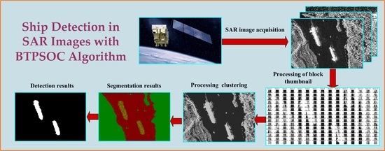
3. Principle Description of the BTPSOC Algorithm

When using the FCM algorithm to effectively detect ship targets in an SAR image, the main difficulty is suppressing speckle noise, setting the initial clustering center, and eliminating the local optimal. To solve these problems, this paper proposes the BTPSOC algorithm. A principle diagram of the BTPSOC algorithm is shown in Figure 1. The algorithm is mainly composed of three functional modules: the main pixels that generate thumbnails; the fuzzy clustering and optimization of thumbnails; and the classification of non-thumbnail pixels.

3.1. Generating Thumbnails

The main ideas related to generating thumbnails are as follows. Firstly, the input image (block image) is processed via iterative clustering, and all the pixels are classified into different pixel groups. Secondly, the main pixel representing the pixel group is obtained according to the histogram’s intensity value of the pixel group. Finally, the average intensity of the main pixels in each pixel group is used to represent the pixels of the thumbnail, and the thumbnail is generated.
The block thumbnail has three advantages: the first is that the size of the block thumbnail is significantly smaller than the original image input; the second is that the thumbnail can represent the features of the input image; and the third is that the thumbnails can reduce the influence of speckle noise.
A simple way to generate thumbnails is via the mean pooling operation, meaning that, for each pixel block in an image, the method represents the entire pixel block through the average value of all its pixels. When segmentation is performed on such a thumbnail, the cost of the operation will be much lower than that of the segmentation on the original input image. However, since the pixels in a square pixel block do not necessarily belong to the same category, using a simple square pixel block as the segmentation unit will lose some useful features. The BTPSOC algorithm divides the input image into different pixel groups based on the feature similarity between the pixels, and, then, uses the pixel groups to generate thumbnails, which can overcome the shortage of feature loss resulting from the simple mean pooling operation. The generation of pixel groups involves three steps, and the specific process is as follows.
Step 1: Take a pixel x i j as the center, and extract a 3 × 3 neighborhood window around it. The amplitude values of all the pixels in the window form a nine-dimensional feature vector f ( x i j ) , which is used to represent pixel x i j . Next, the input image is divided into L × L -size pixel blocks, and these pixel blocks are used to represent the original pixel groups. For each pixel group, the feature vector is the mean of the feature map vectors of all the pixels in the pixel group, and its position is the average position of all the pixels.
Step 2: The pixels in the input image are allocated to the different pixel groups. The center of the pixel group is identified in the N × N   ( N = 2 L 1 ) neighborhood of each pixel, and each pixel is assigned to the pixel group whose center is most similar to its intensity. Pixel similarity can be measured based on the distance d between the pixels. The definition of d is shown in Equation (6), where x i j and x i j represent neighborhood pixels and center pixels, respectively. The smaller the value of d is, the more similar the two pixels are. After all the pixels have been assigned to their corresponding pixel groups, the update phase begins.
d ( x i j , x i j ) = f ( x i j ) f ( x i j ) 2
Step 3: The pixels are updated to obtain new feature vectors and positions. By calculating the mean value of the feature vectors and positions of all the pixels in each group of pixels, the feature vectors and positions of the pixel group are updated. Then, in the next iteration, new feature vectors and positions are obtained according to the pixel groups in the previous iteration, and the feature similarity between each pixel and these new pixel groups is calculated and allocated to the new pixel groups. In this way, after the allocation and update phases have been iterated several times, a group of pixels with similar features can be obtained. In order to intuitively generate pixel groups with similar features, a size of 21 × 21 image is used, as shown in Figure 2.
Figure 2 shows the generation process of pixel groups with similar features. The initial pixel group in the image is a 7 × 7 square block, with the middle pixel of each block acting as the initial center of the pixel group. Each pixel searches for the group of pixels with the most similar features, through Equation (7), in the N × N neighborhood and is subsequently assigned to the appropriate group. When a pixel is assigned to a corresponding group, the pixel is marked with the color of the central pixel in the group. At the end of the algorithm’s iteration, the pixels with the most similar features are assigned to a pixel group and marked with the same color. After the groups of pixels with similar features have been generated, the main pixels in each group are selected to generate the thumbnails.
The maximum and minimum intensity pixels in each pixel group are selected to determine the range of all the pixel values in the group, and, then, the intensity distribution range is divided into G segments. Then, the intensity distribution histogram of the pixel group is established with the divided pixel segment as the horizontal axis. The segment with the largest number of pixels is selected from the histogram, and the pixels in this segment are chosen as the main pixels in this similar pixel group. After the main pixels have been selected, the mean value of the main pixels is used to represent the values of all the pixels in the group of pixels with similar characteristics, and a thumbnail is generated accordingly. Figure 3 shows an original SAR ship image and its generated thumbnail: Figure 3a is the original image and Figure 3b is the thumbnail. The thumbnail not only retains the features of the original image, but also suppresses the noise. The essence of a thumbnail is a block image. If there are not many similar pixels in the image, the difference between the result image and the original image is not significant.

3.2. Thumbnail Pixel Segmentation and Optimization

After the thumbnail of the original SAR image has been obtained, the next step is to segment it effectively. Assume that the thumbnail of the original SAR image is represented by T, and its size is M T × N T , where M T = M / L , N T = N / L , M and N represent the length and width of the original input image, respectively, and L is the size of the block. In the BTPSOC algorithm, the effective segmentation of thumbnails is realized according to the FCM theory. FCM is a nonlinear optimization clustering algorithm based on fuzzy set theory. The process of image segmentation involves constantly updating the cluster center. By constantly iterating to update and modify the cluster center, we ensure that the final output is as close as possible to the real cluster center. Because the FCM algorithm uses a gradient-based local search measure, it easily falls into local minimization and cannot achieve the goal of global optimization. The PSO based on random search is a global optimization algorithm. If it is introduced into the FCM algorithm, it can overcome the defect which allows the FCM algorithm to easily fall into local minimization, improving the clustering accuracy. By using prior information, the scene types in SAR images are preliminarily classified, and the results serve as the initial center of FCM clustering. This initial number of types is used as the initial particle swarm of the PSO algorithm, which then performs a global optimal search, transmits the processing results to the FCM algorithm, and then performs clustering processing. The algorithm repeatedly processes until all the pixels needing to be processed are completed and, finally outputs the clustering result map. The integration of the PSO algorithm into FCM includes two key steps: particle representation and fitness function.

3.2.1. Particle Representation

The position of each particle in the PSO algorithm represents a candidate scheme, which is evaluated using the fitness function value in each iteration. When the fitness function (i.e., the objective function of FCM) of the combined algorithm of FCM and PSO reaches the minimum, the optimal clustering center o j can be obtained, and it is coded as the position p i of the i th particle. This is a candidate scheme. The value range of j is [1, C], and the value range of i is [1, S]. C represents the number of cluster centers, and S represents the number of particles. The vector of C cluster centers can be represented by the position of a particle; that is, the position p i = { h i 1 , h 12 , h i 3 h i c } represents the position of the i th particle and the vector of C cluster centers. h i c represents the vector of the C cluster center at the position of the i th particle. The S group represents multiple candidate clusters of data; namely, the number of groups and cluster centers. A total of S × C variables need to be encoded and decoded. In this method, which combines PSO and FCM, the particle location p i encodes the cluster center o j in it, and the cluster center o j = { h 1 j , h 2 j , h 3 j h s j } can be obtained by decoding the particle location p i . In order to intuitively understand the expression process of particles, Figure 4 describes the expression relationship between four particles— p 1 , p 2 , p 3 , and p 4 —and two cluster centers— o 1 and o 2 —through vector h i j , where i is from one to four and j is from one to two. h i j is similar to parameter d in Equation (6), as h i j is also calculated using Equation (6).

3.2.2. Fitness Function

After the particle representation is completed, the fitness function of the combined PSO and FCM algorithm is designed. The fitness function is defined using the objective function of FCM, as shown in Equation (7).
a i = J F C M = j c i n u i j m d 2 ( z i , o j )
Equation (7) shows that the calculation of the fitness function value includes three steps. First, the cluster center o j ( j = 1 , 2 , 3 c ) is obtained from the previously described particle position representation in Section 3.2.1. Secondly, Equation (2) is used to calculate the membership degree u i j of each element z i in the thumbnail (i.e., the pixels in the thumbnail), and, then, its Euclidean distance d 2 ( z i , o j ) is calculated from the cluster center. Finally, Equation (7) is used to calculate the fitness function value a i of each particle i .
During the implementation of the combined algorithm of FCM and PSO, when the minimum fitness function a i is identified, it is the same as the objective function of minimizing FCM. When the fitness function a i of the combined algorithm is at its smallest, the unlabeled data points in the image will receive optimal classification. At the same time, each data point in the image will achieve optimal segmentation according to its membership degree. The combined algorithm makes full use of the advantages of the FCM and PSO algorithms and seeks the optimal segmentation by minimizing the fitness function value. The position p i and speed v i of each particle i are updated by Equation (4) and Equation (5), respectively. After the thumbnail of the input image has been segmented using the combination algorithm of FCM and PSO, the remaining pixels of the input image are segmented.

3.3. Non-Thumbnail Pixel Segmentation

Block-based image segmentation usually marks the pixels in the block as the same category, often resulting in a loss of detail. In order to make better use of these details, the BTPSOC algorithm will continue to segment the remaining pixels of the input image according to the following three steps. First, the main pixels in the feature pixel group are segmented. Next, the local structure pixels in the pixel group are segmented. Finally, the discrete pixels in the pixel group that are most difficult to classify are segmented.
(1) The first step is to segment the main pixel in the feature pixel group. Because the thumbnail of the input image is constructed according to the average strength and position of the main pixels in the pixel group with similar features, the main pixels in the pixel group should be assigned the same label as the pixels in the thumbnail of the corresponding position. The distribution process is shown in Equations (8) and (9).
l i j = l i ^ j ^ ;    ( i , j ) N i ^ j ^
l i j = 0 ;    ( i , j ) N i ^ j ^
where l i ^ j ^ represents the label of the pixel in the thumbnail of the input SAR ship image; N i ^ j ^ represents the main pixel in the pixel group of the input image corresponding to the position in the thumbnail, and l i j = 0 indicates that the current pixel in the pixel group does not belong to the main pixel and does not assign a label temporarily.
(2) The next step is to segment the local structure pixels in the pixel group. After the main pixels in the input SAR ship image pixel group are segmented, the main part of the remaining pixels in the segmented pixel group consists of the complex local structure pixels. These pixels can be classified in two ways.
The first method consists in assigning labels to the local structure pixels based on the distance between them and the thumbnail cluster center. As shown in Equation (10), we can compare the distance between pixel p i j and each cluster center o j and assign the label of the class with the smallest distance to the pixel.
l p i j = arg min 1 j c p i j o j
The second method consists in using the voting method to assign labels to the local structure pixels. Since most of the pixels in the feature pixel group have been assigned labels after the main pixels in the feature pixel group were segmented, it is possible to search the pixels in the L × L neighborhood centered on the current pixel and assign the labels with the most occurrences to the pixel. As shown in Equation (11), L l represents the set of pixels labeled l in the L × L neighborhood of the current pixel.
l p i j = arg m ax ( L l )
Using the distance method and the voting method described above, each remaining pixel in the input SAR image pixel group is assigned a label based on the corresponding method. If the labels obtained using these two methods are the same, then the current label will be distributed to the pixel. If they are different, the pixels are not assigned labels. The pixels to which tags are assigned during this stage are the complex local structure pixels in the input image. The pixels without labels are the discrete pixels, which will enter the next step of segmentation processing.
(3) Finally, the remaining discrete noise pixels in the feature pixel group are segmented. Once the previous two steps have been completed, the remaining few pixels are called discrete noise pixels. For these pixels, we vote again according to the label results allocated in the previous two steps; the label with more votes is allocated to the pixel. Once the discrete noise pixels have also been segmented, all the pixels in the whole pixel group have obtained their corresponding category labels. At this point, the final segmentation result of the input SAR ship image is achieved.

4. Experimental Results and Analysis

In order to test and validate the correctness and effectiveness of the BTPSOC algorithm, we conducted comparative experiments using actual SAR image data and different methods. In addition to the BTPSOC algorithm, the FCM algorithm, and the PSO algorithm, the fast kernel possibility FCM (FKPFCM) algorithm, CNN, and CFAR methods were also selected for comparative experiments. FKPFCM is an improved FCM algorithm with a fast segmentation speed, fewer computational requirements, and no sensitivity to noise [31].

4.1. Experimental Data and Parameter Setting

4.1.1. Description of Experimental Data

The measured SAR image data used in this paper were obtained from the public SAR ship detection dataset (SSDD) [32] and the SAR-SHIP-SET for detection (SSSD) dataset [33]. There were 1160 SAR images in the SSDD dataset, and each SAR image contained numerous ship targets. The size of each image was 500 × 500. These SAR images were obtained from the Radarsat-2, TerraSAR-X, and Sentinel-1 satellites, respectively. The SAR images of four polarization modes (HH, VV, HV, and VH) were included, and the spatial resolution of the images differed somewhat, ranging from 1 m to 15 m. These ship targets were located both near the edge of the port and far offshore, in the ocean. There were 210 SAR images saved in the SSSD dataset. Of these, 102 SAR images were obtained from the China Gaofen-3 satellite, while the remaining 108 SAR images were obtained from the Sentinel-1 satellite. Each SAR image also contained ship target information. To facilitate the subsequent experimental operations, the original experimental SAR images were cut into slices with a size of 256 × 256. A total of 43,819 SAR image slices were extracted from the datasets.
Some SAR ship images were randomly selected from the two datasets for testing, and the experimental images are shown in Figure 5. The SAR images shown in Figure 5a are from the SSDD dataset. According to the information reflected in the image, the image content could be generally divided into three different regions: sea, ship, and land (port). In Figure 5a, there is a nearshore ship in the first SAR image (Figure 5(a1)). In the second SAR image, there are two medium ships and two small ships (Figure 5(a2)). The third image shows a medium ship and a small ship near the shore (Figure 5(a3)). In the fourth image, there are two fast-moving medium-sized ships (Figure 5(a4)). In the fifth image, there is a large ship near the shore (Figure 5(a5)). The SAR image shown in Figure 5b is from the SSSD dataset, and the information contained in the SAR images is relatively complex. Similarly, these five images can be roughly divided into three different regions: ship, ocean, and land regions. In Figure 5b, there is a small ship in the sea in the first SAR image with a simple background (Figure 5(b1)). In the second SAR image, there are four ships in the sea (Figure 5(b2)). In the third SAR image, there is a medium ship near the shore (Figure 5(b3)). In the fourth image, there are a small and a large ship (Figure 5(b4)), and, in the fifth SAR image, there is a large ship (Figure 5(b5)). The latter three images have a common feature, namely, the image’s signal-to-noise ratio is low and there are a lot of interference information and noise in the image.

4.1.2. Parameter Analysis and Setting

Unsupervised clustering algorithms must fine tune the parameters when searching for the optimal solution in the search space. These parameters are not only particularly important for the algorithm, but also affect the segmentation performance. In the BTPSOC algorithm, the initial clustering number C was initially set according to the number of ground object types in the SAR image coverage area. The experimental image content in this paper is roughly classified into three classes, so the initial clustering number was set to three, namely, C = 3 . Generally, the fuzzy weight value m and the maximum iteration threshold M A X were set to two and thirty, respectively. Other parameters, such as pixel block size L , histogram group number G , particle swarm size S , inertia weight w , cognitive coefficient c 1 , and social coefficient c 2 , would determine the best setting of parameter values by analyzing the performance of the algorithm with regard to the different values. The SAR image shown in Figure 5 was used to analyze the parameter settings, and observe and record the influence of the parameters on the segmentation accuracy and runtime for the different values.
(1) Pixel block size L . The pixel block size L plays a decisive role in the generation of thumbnails and their reduction ratio relative to the original SAR image. The larger the L value is, the smaller the generated thumbnail is, and the shorter the segmentation time is. However, as the L value increases to a certain extent, the pixel details are lost due to the mean operation, which affects the final segmentation effect. See below for a detailed experimental analysis process for L to select different values.
First, we fix the other five parameter values ( G , S , w , c 1 , and c 2 ), and, then, when L takes a specific value, the average accuracy and the average runtime of the SAR image segmentation result map will be calculated after the algorithm has been executed 10 consecutive times. When the parameter L takes different values, the changes in the algorithm’s performance indicators ACC and Time are shown in Figure 6a and Figure 6b, respectively.
Figure 6 shows that, with the increase in pixel block size L , the segmentation accuracy value of the algorithm initially increases and then decreases, and that the execution time of the algorithm decreases continuously. Therefore, the value of L should minimize the runtime of the algorithm under the condition that the algorithm has a better accuracy. Therefore, the value of L should keep the runtime of the algorithm as short as possible, assuming that the algorithm has better accuracy. In Figure 6, the analysis of the performance under different L values reveals that, when the value of parameter L is five, the effect of the algorithm is at its best. At this value, the segmentation accuracy value is at its highest and the runtime is shorter.
(2) Number of histogram groups G . In order to select the main pixels to generate thumbnails, the number of pixels in each range is calculated by building an intensity histogram of pixel values. The number of histogram groups G is directly related to the selection of main pixels. If the G value is small, most of the pixels in the pixel group are distributed in a histogram group; these are called primary pixels. At this time, the number of remaining pixels in the pixel group is relatively small. On the contrary, if the number of main pixels of the pixel group is relatively small, then more pixels remain. These two situations are not conducive to the effective segmentation of image pixels. The selection process of the histogram group number G is described below.
We fix the other five parameter values ( L = 5 , S , w , c 1 , c 2 ) and, then, run the BTPSOC algorithm multiple times with different sizes of the histogram group G . Next, we select ten maps of the segmentation results and calculate the average segmentation accuracy, the runtime, and the percentage of remaining pixels (PRP) in the pixel group ten times. Figure 7a–c show the change curves of ACC, time, and PRP when G takes different values.
In Figure 7a, when the parameter value G increases, the ACC value of the SAR images constantly decreases as a result. Additionally, the ACC value is highest when G = 3 . Figure 7b shows that G has little impact on the runtime of the BTPSOC algorithm. In Figure 7c, when the value of G is three, the remaining pixels in the pixel group comprise about 20% of the image pixels, which means that 80% of the pixels in the pixel group are the main pixels, and the segmentation task is completed in the first step of the remaining pixel segmentation performed using the BTPSOC algorithm. When the value of G is 13, the remaining pixels in the pixel group comprise about 45% of the total pixels in the image. This means that 45% of the pixels in the pixel group will remain in the second and the third steps of the remaining pixel segmentation in the BTPSOC algorithm to complete the segmentation task. This will lead to poor segmentation results because it will ignore the effective information of the image. Thus, it can be inferred from Figure 7 that, in order to achieve the best performance of the algorithm, the G value should be set to three.
(3) Particle swarm size S . In order to obtain an appropriate particle swarm size S , we fix the remaining parameters ( L = 5 , G = 3 , w , c 1 , and c 2 ), and then perform processing 10 times, respectively, under the condition that S takes different size values. We calculate the segmentation accuracy value ACC for each time and, then, average the results of the 10 experiments as the current result. Table 1 shows the accuracy values of the algorithm on SAR images under different values of S . As shown in Table 1, at the beginning, the ACC value gradually increases with the particle swarm size. When S = 60 and A C C = 0.851 , the ACC value is at its maximum. Then, as the number of particle swarm continues to increase, the ACC value decreases instead. Therefore, when S = 60 , the algorithm achieves its best segmentation accuracy.
(4) Inertia weight w . In order to determine the inertia weight value w , we fix other parameters ( L = 5 , G = 3 , S = 60 , c 1 , and c 2 ); then, when w takes different values, the BTPSOC algorithm is executed ten consecutive times and the average accuracy is calculated. The results are shown in Table 2. It is clear that the ACC value gradually increases with the increase in the weight value w . However, when the weight value exceeds one, the ACC value decreases instead. Therefore, when w = 1 , the algorithm achieves its best segmentation performance.
(5) Cognitive coefficient c 1 and social coefficient c 2 . In order to set the values of c 1 and c 2 , we begin by fixing other parameters ( L = 5 , G = 3 , S = 60 , and w = 1 ). Then, when c 1 and c 2 take different values, the BTPSOC algorithm is run ten consecutive times and the average accuracy of the segmentation maps is calculated. Table 3 shows the detailed experimental results. Based on these results, it is evident that, when the values of c 1 and c 2 are equal to two, the BTPSOC algorithm can achieve its best segmentation accuracy and performance.

4.2. SAR Image Experimental Results of the SSDD Dataset

4.2.1. Evaluation Index of Experimental Results

Ship target detection in SAR images essentially involves segmenting and extracting the target region (ship) from the image background (non-ship). Therefore, image target detection is a binary classification problem in which an image’s pixels are ultimately attributed to either the target region or the background region. The class containing the target region (ship) is called a positive class, while the class containing the background region (other than the ship) is called a negative class. When matching the detection results with the actual situation, either a correct classification or an incorrect classification will occur, and the classification will be identified as true or false, respectively. If the pixel extracted from the ship region is deemed to be the ship target, the pixel is classed as a true positive (TP); if it is deemed to be a non-ship target, but is in fact a ship target region pixel, the pixel is assigned to the false negative (FN) class. If the extracted background region pixels are correctly identified as belonging to background classes, they are assigned to the true negative (TN) class; if a background pixel is mistakenly identified as a pixel in the target region of the ship, this pixel is assigned to a false positive (FP) class. For an SAR image containing ship targets, if the true positive class value of the target area or the true negative class value of the background area is higher, the correct detection rate of the ship target area is higher, and the correct segmentation accuracy of the target region is also higher. There are many evaluation indicators for the detection and segmentation effect of image target regions, and commonly used indicator parameters include recall (REC) rate, precision (PRE) rate, F-Measure (FM), accuracy (ACC) rate, receiver operating characteristic (ROC) curve, and area under curve (AUC). Note that the curve here refers to the receiver operating characteristic curve. The calculation equations for the four parameters of the former are as follows.
R E C = T P T P + F N
P R E = T P T P + F P
F M = 2 P R E × R E C P R E + R E C
A CC = T P + T N T P + T N + F P + F N
The recall rate refers to the segmentation performance of ship target pixels: the recall index indicates the number of ship target region pixels that have been truly segmented. The precision rate indicates the ratio between the number of correctly predicted positive samples and the number of predicted positive samples, which is a segmentation evaluation indicator pertaining to the precision. The F-Measure represents the harmonic average value of the recall and the precision, which is used to comprehensively reflect the overall situation. This is because the higher the REC and the PRE values, the better the classification effect of the image pixel type. However, it is very difficult to simultaneously achieve high values for both. At this time, only the FM parameter can be used for comprehensive harmonic evaluation. The accuracy rate refers to the correct segmentation accuracy of the whole image. It represents the accuracy of the entire image pixels classification. The ROC is a parameter indicator that is used to evaluate the convergence efficiency of image segmentation algorithms. Generally, the faster the curve convergence, the better the classification effect. Similarly to the ROC curve, the AUC parameter is also an index that can be used to evaluate the performance of the image segmentation algorithm. The larger the AUC value, the closer the receiver operating characteristic is to the upper left corner, the better the convergence of the algorithm, and the better the image segmentation effect.

4.2.2. Segmentation Results of Different Methods

The original experimental images are shown in Figure 8A–E, and they correspond to Figure 5(a1–a5), respectively. Since the imaging scenes of the SAR images selected from the SSDD dataset mainly included ship, sea, and land, the initial number of clusters of these algorithms was set to three. Figure 8A–E denote the SAR images of different scenes, i.e., original images (Figure 8a). Figure 8b represents the truth scene on the ground, and Figure 8c–f represent the experimental results obtained by the FCM, PSO, FKPFCM, and BTPSOC algorithms, respectively. In the experiment, the lands containing different ground objects are divided into land uniformly, without subdivision, because the purpose of the experiment was to detect the ship target instead of just image segmentation. In order to improve the visual effect, different regions (different classes) in the segmentation result were represented using different colors.
The results of the FCM algorithm’s processing are shown in Figure 8c. For the SAR image shown in Figure 8A, the segmentation result (Figure 8(c1)) is hollow; the ship edge is incomplete; and the land is wrongly classified as a ship. For the image shown in Figure 8B, there are holes in the segmentation results (Figure 8(c2)) and small ships are missed. Additionally, there are cavities and incomplete edges in the segmentation result (Figure 8(c3)) for Figure 8C. In Figure 8D, the edge of the ship in the segmentation result (Figure 8(c4)) is incomplete and the land (island) is divided based on the ships. For the image shown in Figure 8E, the edges of the ship in the segmentation result (Figure 8(c5)) are incomplete and there are holes. In other words, if the FCM algorithm is used to detect the ship targets in the SAR images of the SSDD dataset, the detection effect and visual effect are relatively poor.
The experimental results obtained using the PSO algorithm are shown in Figure 8d. Figure 8(d1) shows that the edge of the ship in the detection result is incomplete and that there are holes. Many of the land areas are divided into ships, and some of the areas are classified as oceans. In Figure 8(d2), the edge segmentation of the ship is incomplete; there is a hole in the middle; the ship close to the land is leaked, and the noise in the sea is classified as land. In Figure 8(d3), not only is the edge of ship detection incomplete, but also the second ship is divided into two parts. Several of the land areas are classed as sea, and the noise in the sea is divided into ships. In Figure 8(d4), the edge of the ship is incomplete and some islands in the sea are classified as ships. The inconspicuous features in the land are divided into the sea surface. In Figure 8(d5), the ship has incomplete edges and strip cavities. The land is mistakenly measured as sea surface and ship, and the sea surface’s noise is also classified as land and ship. Through the analysis of the above experimental results, it is concluded that the PSO algorithm and the FCM algorithm produce similar results and that their effect on SAR image target segmentation is not ideal.
The images in Figure 8e were obtained using the FKPFCM algorithm. Figure 8 indicates that the overall experimental results of the FKPFCM algorithm are better than those obtained using the FCM and PSO algorithms. As shown below, for Figure 8(e1), the edges of the ship in the segmentation result are incomplete and there are holes. In the segmentation result of the image shown in Figure 8(e2), the ship not only has incomplete edges, but also has holes, and some areas remain undetected. For Figure 8(e3), although the edge of the ship is incomplete, there is no case in which the ship is isolated. For the segmentation result of the image shown in Figure 8(e4), although the edges of the ship are incomplete, only a few islands are wrongly detected as ships. At the same time, the land is wrongly identified as an ocean area with relatively low frequency. In the segmentation result of the image shown in Figure 8(e5), although the edges of the ship are incomplete, the size and number of cavities are reduced and the land is not mistaken for a ship. According to the above description and analysis, the experimental results that the FKPFCM algorithm has obtained are better than those of the FCM and PSO algorithm in terms of visual effect representation.
Figure 8f shows the experimental results of the BTPSOC algorithm proposed in this paper. As shown in Figure 8, the experimental results obtained using the BTPSOC algorithm are better than the previous three algorithms in terms of visual effects. In the processing of Figure 8(f1), the edge details of the ship are more complete; the holes become smaller, and the land wrongly classified as ocean is also smaller. In Figure 8(f2), the edge of the ship is relatively perfect; there is only one hole, and small ships are also correctly detected. Only two of the land areas are wrongly classified as oceans. For Figure 8(f3), there is no cavity in the ship and the edges are relatively complete. A piece of land in the lower right corner is wrongly classified as ocean. In Figure 8(f4), the edge structure of the ship is complete without holes and the islands in the sea are not incorrectly classified as ships. There is no case in which the land is wrongly classified as sea. For Figure 8(f5), the edge structure of the ship is complete, with only one cavity. At the same time, the land is not wrongly classified as sea.
Analysis of the above experimental results shows that the FCM and PSO algorithms had the worst performance in terms of intuitive visual effects, whether in the edge structure or in the internal cavity of the ship, and that the land and the sea were often incorrectly classified. Because a single FCM algorithm is easily affected by local noise, it is easy to generate incorrect segmentation results for images containing noise. Noise with larger amplitude values can affect the FCM algorithm’s selection of clustering centers, resulting in new types (different regions) and inaccuracies in the final segmentation results. The PSO algorithm is used to process image segmentation by making individual judgments on pixels and then assigning them to which particle swarm (class). A single pixel is easily affected by noise, so the PSO algorithm is also bound to be affected by noise, especially the speckle noise in SAR images, which leads to unsatisfactory segmentation results. The FKPFCM algorithm offers a certain level of improvement compared to the previous two algorithms, but fails to achieve the desired effect. The best performance is achieved by the BTPSOC algorithm. In the experimental results, the ship structure is relatively complete, with few holes. The classification result is more accurate than that of the previous three algorithms and closer to the real scene on the ground. This is because the pixel groups of similar sizes created using the BTPSOC algorithm and the global optimization of PSO improve the accuracy of pixel classification.

4.2.3. Quantitative Analysis and Comparison

Next, from the perspective of parameters, we performed a quantitative analysis of the four experimental methods used earlier to further evaluate their performance in detail. Firstly, the performance of the algorithm was analyzed via a visual histogram of the evaluation indicators REC, FM, ACC, and PRE. Then, the ROC curve and AUC value were used for comparison and analysis. Finally, the runtime of various algorithms was analyzed.
Figure 9 shows the REC values of the segmentation result maps of the SAR images in the SSDD dataset according to the four algorithms in Figure 8. Figure 9 shows that, among all the experimental result images, the REC value that is obtained using the PSO algorithm is the lowest, indicating that its segmentation performance is poor with regard to SAR image ship target detection. The maximum value of REC is obtained using the BTPSOC algorithm, which shows that the algorithm is highly effective when processing SAR ship targets images. The next-largest value is obtained using the FKPFCM algorithm, followed by the FCM algorithm. In Figure 9, according to the size of the parameter recall value, it can be inferred that the performance of the BTPSOC, FKPFCM, FCM, and PSO algorithms for target region detection is gradually reduced.
The PRE values of the segmentation results’ maps using the four algorithms are shown in Figure 10. The figure shows that the FKPFCM algorithm is the best out of the previous three algorithms, with a PRE value reaching 0.8095. In contrast, the values achieved by the segmentation results’ maps of the BTPSOC algorithm are the highest for the different images, and the highest reached 0.8995. This means that the precision of the BTPSOC algorithm for ship target segmentation in SAR images is good. The precision values of the FCM and PSO algorithms are not only the lowest, but also very close, which indicates that their classification effects on SAR images are relatively poor.
Figure 11 shows the F-Measure values of the segmentation result images, which are obtained using different algorithms. It is obvious in Figure 11 that the PSO algorithm obtains the minimum FM value, and, in Figure 8A, its F-measure value is only 0.6325. The FCM algorithm is close to the PSO algorithm, so its FM value is low but remains slightly higher than the PSO algorithm’s. Figure 11 shows that, for all the experimental images, the FM values obtained using the FCM algorithm and the PSO algorithm are relatively low, indicating that the segmentation effect of these two algorithms for SAR images is relatively poor. As a result, they are used to segment SAR images directly and their performance is poor. The FM values calculated using the BTPSOC algorithm for the segmentation and detection result images of ship targets in the different SAR images are relatively high, much higher than those of the second FKPFCM algorithm. This shows that the segmentation effect of the BTPSOC algorithm is satisfactory, stable, and has a good universality.
The segmentation accuracy values of the segmentation results of the different algorithms on the different images analyzed are shown in Figure 12. The change rule of ACC is the same as that reflected by the previous three performance indicators: REC, PRE, and FM. The ACC value of the PSO algorithm is at its minimum. For example, in Figure 8E, its ACC value is only 0.7501, which means that the classification of ship, land, and sea in the SAR images is poor. The ACC value of the FCM algorithm is very close to that of the PSO algorithm. The second-highest value algorithm of ACC is obtained using the FKPFCM algorithm, and its ACC value in Figure 8E is 0.8189. The best performance is the BTPSOC algorithm’s, from the point of view of the ACC parameter’s values. The highest ACC value obtained using this algorithm is 0.8824, as shown in Figure 8C.
The ROC curves obtained from the segmentation result images of Figure 8A–E using different algorithms are shown in Figure 13. Here, Figure 13a–e show the experiments of five groups of data, respectively, and the corresponding original SAR images are shown in Figure 8A–E. As shown in Figure 13c,e, the ROC curve obtained on the SAR image converges faster because the difference between the ship and the surrounding environment in these two images is clear and the noise level of the image is relatively low. It is noted that, regardless of the image, the trend of the ROC curves of the FCM and PSO algorithms is similar and close to the diagonal, indicating that their accuracy with regard to ship target detection in the SAR images is low. In addition, it is obvious that the ROC curves of the FKPFCM and BTPSOC algorithms are close to the upper-left corner of the graph, indicating that the segmentation accuracy of these two algorithms is higher than that of the FCM and PSO algorithms. In particular, the proposed BTPSOC algorithm is closer to the upper-left corner of the graph than the FKPFCM algorithm and has obvious differences, which shows that the BTPSOC algorithm has the highest segmentation accuracy in the SAR image ship detection with the SSDD image data.
Table 4 shows the mean and standard deviation of the AUC parameters under the ROC curve obtained using each algorithm on the image processed in Figure 8A–E. As shown in Table 4, the mean of the AUC obtained using the FCM algorithm is 73.52% and the standard deviation is 3.26%. The mean and variance of the AUC obtained using the PSO algorithm are 72.15% and 3.54%, respectively, which are similar to those of the FCM algorithm. Its mean is slightly smaller than that of the FCM algorithm and its variance is slightly larger than that of the FCM algorithm. The highest mean value of the AUC is achieved using the BTPSOC algorithm, reaching 89.51%, followed by the FKPFCM algorithm, whose value is 81.43%. Meanwhile, the standard deviation of the BTPSOC algorithm is the smallest, i.e., 1.52%, which shows that it not only has high accuracy in segmentation and ship target detection, but also is a relatively stable algorithm.
The complexity of algorithms is mainly reflected by their storage capacity and runtime. Previously, a specific quantitative analysis was conducted according to the different parameters; the runtime of the different algorithms will be discussed next. Figure 14 shows the average time the different algorithms have taken to complete the same image segmentation operation. To compare the execution time of the various algorithms, segmentation experiments were carried out on the test SAR images. The average execution time of the various algorithms were recorded and calculated, and the experimental results are shown in Figure 14. The runtime of the FCM algorithm and the PSO algorithm are relatively close; the FKPFCM algorithm has the longest runtime, and the BTPSOC algorithm has the shortest runtime at 5.61s. This experiment shows that the BTPSOC algorithm is more efficient than the other three algorithms when it comes to processing the SAR images from the SSDD dataset and that it has the shortest runtime. This indicates that the BTPSOC algorithm can reduce runtime and improve operational efficiency.
From the experimental results and quantitative analysis above, it can be seen that the BTPSOC algorithm has been improved to a certain extent: for instance, using thumbnail images to generate block regions can reduce the impact of noise, while the PSO algorithm can improve the accuracy of search. These two aspects jointly promote the improvement of the BTPSOC algorithm’s performance.

4.2.4. Comparison with CNN Methods

The deep convolutional neural network theory is currently the most active frontier in data prediction and classification algorithms. For example, the FCN and U-Net networks are two deep neural network methods that are often used for image semantic segmentation [34,35,36]. Therefore, we performed an experiment to compare the BTPSOC algorithm and these two deep learning methods. The experimental results are shown in Figure 15 and Table 5. Figure 15a shows the original SAR image, which is the image shown in Figure 8E. Figure 15b–d show the segmentation results of the FCN, U-Net, and BTPSOC algorithms, respectively. The FCN and U-Net models were trained using images from the SSDD database. The relevant parameter settings for the training are as follows. There are 2000 iterations, with batch sizes of 50. The learning rate is updated based on the number of iterations, which are determined based on the stage. The initial learning rate is set to 0.001, and, when the number of iterations exceeds 500, the learning rate is adjusted to 0.0005. When the number of iterations exceeds 1200, the learning rate is adjusted to 0.0001.
Judging by the visual effect, Figure 15b is the closest to Figure 15a, followed by Figure 15c, and, finally, Figure 15d. From the perspective of image pixel classification or segmentation, the FCN algorithm has the highest segmentation accuracy, followed by the U-Net algorithm, and the BTPSOC algorithm has the lowest accuracy. Table 5 contains the values of the two evaluation parameters, ACC and REC, used to obtain the results shown in Figure 15. The REC is a recall index, which indicates how many pixels in the target region have been extracted. In this experiment, it refers to the correct detection rate of pixels in the ship target region. Table 5 shows that the REC parameter value of the BTPSOC algorithm is the largest. When detecting the ship’s target region, this method is superior to the other two deep learning methods. However, judging from the pixel type’s semantic segmentation performance and the value of the segmentation accuracy indicator ACC of the whole image, the FCN algorithm has the largest value, while the U-Net algorithm has a slightly smaller value, and the BTPSOC algorithm has the smallest value. The results of these comparative experiments show that the BTPSOC method is better, based on the detection and segmentation of target regions, and that the FCN algorithm and U-Net algorithm are better based on image semantic segmentation. However, the FCN and U-Net methods require a large number of sample images to train the complex models, consuming a lot of time and storage space, and different data samples and models will also affect their segmentation accuracy and runtime. Therefore, the advantages of the BTPSOC algorithm will be more prominent for few or single SAR images. Through this experiment, we can draw a preliminary conclusion that a deep convolutional neural network method is suitable for an image’s semantic segmentation with a large amount of training samples data. Additionally, the BTPSOC algorithm is only suitable for situations with only a small amount of sample data and a single SAR image. Since it does not require prior knowledge for image processing, it is very suitable for the detection and analysis of ship targets in SAR images.

4.2.5. Comparison with the CFAR Method

The constant false alarm rate (CFAR) method is frequently used during object detection. After years of development, CFAR not only developed many branch theories, but also inspired a large number of improved algorithms. Common methods include the cell average CFAR (CA-CFAR), the smallest of CFAR (SO-CFAR), the greatest of CFAR (GO-CFAR), the order statistical CFAR (OS-CFAR), and the two-parameter CFAR (TP-CFAR) [37]. Many false alarm detection algorithms are based on the improvement of CA-CFAR, so, in this experiment, the CA-CFAR method was chosen for the experiments. In practical applications, good detection results can generally be achieved when the application conditions are met. As such, this algorithm is usually used for comparative analysis. Similarly, as a non-intelligent method, the BTPSOC algorithm was also compared with traditional CA-CFAR in experiments, and the experimental results are shown in Figure 16.
Figure 16a is the original SAR image, while Figure 16b–d shows the results obtained using the CA-CFAR method, and Figure 16e is a result of the BTPSOC algorithm. Figure 16b shows the result of directly detecting images (Figure 16a) using the CA-CFAR method. The result shown in Figure 16c was also obtained using the CA-CFAR method, but it was filtered using a 5 × 5 window prior to detection. Additionally, the false alarm rate used was 1 × 10⁻⁵. Figure 16d is the result obtained after mask processing on Figure 16c. Figure 16 shows that CA-CFAR can effectively detect ship targets, but it cannot distinguish between ship targets and land targets. Further measures must be taken to fully detect the target area. As the prerequisite for the CFAR method to effectively detect targets is that there must be a significant difference between the target area and the background area, otherwise its overall detection effect is relatively poor.

4.3. Experimental Results of the SSSD Dataset Images

In order to further test the feasibility and universality of the BTPSOC algorithm, after completing the qualitative and quantitative analysis and comparison experiments of different algorithms on the SSDD data, we performed segmentation experiments on the SAR images in the SSSD dataset with the different algorithms. The experimental images and results are shown in Figure 17. Here, Figure 6A–E represent the original SAR images of the SSSD dataset, which are the images shown in Figure 5(b1–b5). Figure 17a,b show the original image and the ground truth, respectively. Figure 17c–f show the experimental results obtained using the PSO, FCM, FKPFCM, and BTPSOC algorithms, respectively.
Figure 17c demonstrates that the visual effect of the experimental result map obtained using the PSO algorithm is less than ideal, as shown below. In Figure 17(c1), the ship edge is incomplete and the land is wrongly classified as a ship because the pixels used to denote the ship and the land are very similar in this image. The land protruding from the upper left corner is misclassified as ships, and two ships are overlooked in Figure 17(c2). In Figure 17(c3), due to the strong speckle noise on the land, the land in the middle is wrongly classified as a ship and part of the land on the left is classified as a sea surface. At the same time, the noise in the sea is divided into land and there is a hole in the upper-right corner of the ship. In Figure 17(c4), the land connecting ships is wrongly classified as ships; the noise from the sea is wrongly classified as land, and the segmentation edge of the ship is incomplete. In the image shown in Figure 17(c5), the strip land on the right is wrongly divided into ships and the noise in the sea is divided into land.
The experimental results shown in Figure 17d were obtained using the FCM algorithm. Figure 17 shows that the segmentation result of the FCM algorithm is very similar to results obtained using the PSO algorithm. For example, in Figure 17(d1), the edge of the ship in the image segmentation result is incomplete; the land is wrongly classified as sea and ship, and the speckle noise in the sea is classified as land. For Figure 17(d2), only a small part of two ships is detected; part of the land is classified as sea, and the protruding part of the land is incorrectly identified as a ship. In Figure 17(d3), the edge of the ship in the image segmentation result is incomplete. The land area contains the pixels from the ship and the sea and the sea area also contains land pixels. In the image shown in Figure 17(d4), the ship structure in the segmentation result is incomplete and the regions with strong pixels in the land are divided into ships. The middle part of the land is divided into the sea. Due to the influence of noise, some of the pixels in the sea area are divided into land. In Figure 17(d5), some of the land pixels are wrongly classified as ships and the sea surface around the ships is incorrectly classified as land due to noise.
The experiment result of the FKPFCM algorithm is shown in Figure 17e. It is evident that the FKPFCM algorithm is vastly superior to the PSO and FCM algorithms in the segmentation result map. For example, the integrity of the ship edge structure is improved; the holes in the ship area are reduced; the undetected ships are identified; the pixels of the land that is incorrectly classified as ships and the sea are reduced, and the areas in the sea that are wrongly classified as land are also reduced.
The experimental results obtained using the BTPSOC algorithm are shown in Figure 17f. As shown in Figure 17, the segmentation effect of the BTPSOC algorithm is the best among the used experimental algorithms. According to the processing results of the images shown in Figure 17c–f, in the result image segmented using the BTPSOC algorithm, the edge structure of the ship is close to the true value; the hole is small, and the detection is complete. A pixel of the land area is wrongly classified as ship and sea surface, which occurs much less frequently than is observed for the previous three methods. The sea area is also incorrectly divided into land less frequently.
After a detailed analysis of the experimental results of the SAR images in the SSSD dataset, a preliminary conclusion can be drawn. The best visual effect can be achieved using the BTPSOC algorithm, followed by the FKPFCM algorithm, the FCM algorithm, and the PSO algorithm. At the same time, the evaluation parameter indicators such as REC, PRE, FM, ACC, ROC, and AUC and the runtime are also used to compare and analyze the experimental results obtained using the different methods. The rules reflected by these parameters are very similar to those in the SSDD dataset.

4.4. Complexity and Robustness Analysis

The runtime of the BTPSOC algorithm is shorter than that of the FCM, PSO, and FKPFCM algorithms. The main reason is that the original SAR images in the BTPSOC algorithm construct the block thumbnails through feature-similar pixel groups. If the pixel size of the input SAR image is M × N , the pixel size of the constructed block thumbnail is ( M / L ) × ( N / L ) . The number of pixels of the block thumbnail is much smaller than that of the original SAR image. While processing SAR images using the BTPSOC algorithm, the time complexity of getting the block thumbnails is O ( M × N ) , but the time complexity of segmenting thumbnails is O ( M / L × N / L ) . Finally, the time complexity of the algorithm on the input SAR image is determined by the complexity of generating block thumbnails, which is O ( M / L × N / L ) . Therefore, the block thumbnails can reduce the time complexity when the BTPSOC algorithm segments a SAR image.
To verify the stability of the BTPSOC algorithm, the algorithm was executed 30 times on each of the SAR shown in Figure 8A–E, and the minimum, maximum, mean, and standard deviation of the ACC values of each segmentation’s result map were recorded and calculated, respectively. The results are shown in Table 6. As shown, no matter how drastically the SAR image content changes, the fluctuation in the segmentation accuracy value of the BTPSOC algorithm on each image remains relatively small. The difference between the maximum value and the minimum value is small, and the standard deviation is also very small. This shows that the segmentation processing of the BTPSOC algorithm on the SAR ship image is relatively stable; the robustness of the algorithm is good, and there will be no large fluctuations resulting from different execution times.

5. Conclusions

Ship target detection is an important aspect of ocean monitoring management and one of the numerous applications of SAR images. Therefore, using SAR images to detect ship targets is an important research focus. Aiming to mitigate the shortcomings of traditional mean clustering segmentation algorithms, this paper proposed a new ship target detection algorithm based on block thumbnail and particle swarm optimization clustering with SAR images. Our proposed algorithm can improve the running speed and detection accuracy, and it also suppresses noise. The semantic segmentation learning algorithm based on the CNN model can achieve high classification and segmentation accuracies, but it is not optimal for the detection of target regions and needs to collect and train a large number of sample image data prior to its implementation. On the contrary, for the target detection of a small sample of SAR image data, the BTPSOC algorithm has more obvious advantages and excellent application value. In future work, we will combine the concept of the BTPSOC algorithm with deep learning theory to improve the automatic detection and intelligent processing of SAR ship targets.

Author Contributions

Conceptualization and methodology, S.H.; software, S.H.; formal analysis, O.Z.; investigation, Q.C.; resources and data curation, S.H.; writing—original draft preparation, S.H.; writing—review and editing, O.Z.; visualization, O.Z.; supervision, Q.C.; project administration, S.H.; funding acquisition, S.H. All authors have read and agreed to the published version of the manuscript.

Funding

This research was funded by the Natural Science Foundation of China (No. 41574008, 61379031, and 61673017), and it was funded by the Guangdong Province Key Construction Discipline Scientific Research Capacity Improvement Project (2022ZDJS135).

Data Availability Statement

The data presented in this study are available on request from the corresponding author.

Conflicts of Interest

The authors declare no conflict of interest. The funders had no role in the design of the study; in the collection, analyses, or interpretation of the data; in the writing of the manuscript; or in the decision to publish the results.

References

  1. Saha, S.; Bovolo, F.; Bruzzone, L. Building change detection in VHR SAR images via unsupervised deep transcoding. IEEE Trans. Geosci. Remote Sens. 2021, 59, 1917–1929. [Google Scholar] [CrossRef]
  2. Allies, A.; Roumiguié, A.; Fieuzal, R.; Dejoux, J.-F.; Jacquin, A.; Veloso, A.; Champolivier, L.; Baup, F. Assimilation of multisensor optical and multiorbital SAR satellite data in a simplified agrometeorological model for rapeseed crops monitoring. IEEE J. Sel. Top. Appl. Earth Obs. Remote Sens. 2021, 15, 1123–1138. [Google Scholar] [CrossRef]
  3. Lê, T.T.; Froger, J.-L.; Minh, D.H.T. Multiscale framework for rapid change analysis from SAR image time series: Case study of flood monitoring in the central coast regions of Vietnam. Remote Sens. Environ. 2022, 269, 112837. [Google Scholar] [CrossRef]
  4. Shi, J.C.; Xu, B.; Chen, Q.; Hu, M.; Zeng, Y. Monitoring and analysing long-term vertical time-series deformation due to oil and gas extraction using multi-track SAR dataset: A study on lost hills oilfield. Int. J. Appl. Earth Obs. Geoinf. 2022, 107, 102679. [Google Scholar] [CrossRef]
  5. Zhang, C.; Gao, G.; Zhang, L.; Chen, C.; Gao, S.; Yao, L.; Bai, Q.; Gou, S. A novel full-polarization SAR image ship detector based on scattering mechanisms and wave polarization anisotropy. ISPRS J. Photogramm. Remote Sens. 2022, 190, 129–143. [Google Scholar] [CrossRef]
  6. Abdikan, S.; Sekertekin, A.; Madenoglu, S.; Ozcan, H.; Peker, M.; Pinar, M.O.; Koc, A.; Akgul, S.; Secmen, H.; Kececi, M.; et al. Surface soil moisture estimation from multi-frequency SAR images using ANN and experimental data on a semi-arid environment region in Konya, Turkey. Soil Tillage Res. 2023, 228, 105646. [Google Scholar] [CrossRef]
  7. Cao, X.; Gao, S.; Chen, L.; Wang, Y. Ship recognition method combined with image segmentation and deep learning feature extraction in video surveillance. Multimedia Tools Appl. 2020, 79, 9177–9192. [Google Scholar] [CrossRef]
  8. Zhang, X.; Dong, G.; Xiong, B.; Kuang, G. Refined segmentation of ship target in SAR images based on GVF snake with elliptical constraint. Remote Sens. Lett. 2017, 8, 791–800. [Google Scholar] [CrossRef]
  9. Proia, N.; Pagé, V. Characterization of a Bayesian ship detection method in optical satellite images. IEEE Geosci. Remote Sens. Lett. 2009, 7, 226–230. [Google Scholar] [CrossRef]
  10. Wang, X.Q.; Zhu, D.; Li, G.; Zhang, X.-P.; He, Y. Proposal-copula-based fusion of spaceborne and airborne SAR images for ship target detection. Inf. Fusion 2022, 77, 247–260. [Google Scholar] [CrossRef]
  11. Zhang, T.W.; Xu, X.W.; Zhang, X.L. SAR ship instance segmentation based on hybrid task cascade. In Proceedings of the 18th International Computer Conference on Wavelet Active Media Technology and Information Processing (ICCWAMTIP), Chengdu, China, 17–19 December 2021; pp. 530–533. [Google Scholar]
  12. Li, J.C.; Gou, S.P.; Li, R.M.; Chen, J.-W.; Sun, X. Ship segmentation via encoder-decoder network with global attention in high-resolution SAR images. IEEE Geosci. Remote Sens. Lett. 2021, 19, 1–5. [Google Scholar] [CrossRef]
  13. Hou, X.; Ao, W.; Xu, F. End-to-end automatic ship detection and recognition in high-resolution gaofen-3 spaceborne SAR images. In Proceedings of the 2019 IEEE International Geoscience and Remote Sensing Symposium (IGARSS), Yokohama, Japan, 28 July–2 August 2019; pp. 9486–9489. [Google Scholar]
  14. Perdios, D.; Vonlanthen, M.; Martinez, F.; Arditi, M.; Thiran, J.-P. CNN-based image reconstruction method for ultrafast ultrasound imaging. IEEE Trans. Ultrason. Ferroelectr. Freq. Control 2022, 69, 1154–1168. [Google Scholar] [CrossRef] [PubMed]
  15. Yao, Y.; Yan, X.Q.; Luo, P.; Liang, Y.; Ren, S.; Hu, Y.; Han, J.; Guan, Q. Classifying land-use patterns by integrating time-series electricity data and high-spatial resolution remote sensing imagery. Int. J. Appl. Earth Obs. Geoinform. 2022, 106, 102664. [Google Scholar] [CrossRef]
  16. Long, J.; Shelhamer, E.; Darrell, T. Fully convolutional networks for semantic segmentation. In Proceedings of the IEEE Conference on Computer Vision and Pattern Recognition, Boston, MA, USA, 7–12 June 2015; pp. 3431–3440. [Google Scholar]
  17. Nie, X.; Duan, M.; Ding, H.; Hu, B.; Wong, E.K. Attention mask R-CNN for ship detection and segmentation from remote sensing images. IEEE Access 2020, 8, 9325–9334. [Google Scholar] [CrossRef]
  18. Zhang, W.; He, X.; Li, W.; Zhang, Z.; Luo, Y.; Su, L.; Wang, P. An integrated ship segmentation method based on discriminator and extractor. Image Vis. Comput. 2020, 93, 103824. [Google Scholar] [CrossRef]
  19. Otsu, N. A threshold selection method from gray-level histograms. IEEE Trans. Syst. Man Cybern. 2007, 9, 62–66. [Google Scholar] [CrossRef]
  20. Kittler, J.; Illingworth, J. Minimum error thresholding. Pattern Recognit. 1986, 19, 41–47. [Google Scholar] [CrossRef]
  21. Yu, H.; Jiao, L.C.; Liu, F. Context based unsupervised hierarchical iterative algorithm for SAR segmentation. Chin. Acta Autom. Sin. 2014, 40, 100–116. [Google Scholar]
  22. Jin, D.R.; Bai, X.Z. Distribution information based intuitionistic fuzzy clustering for infrared ship segmentation. IEEE Trans. Fuzzy Syst. 2020, 28, 1557–1571. [Google Scholar] [CrossRef]
  23. Shang, R.H.; Chen, C.; Wang, G.G.; Jiao, L.; Okoth, M.A.; Stolkin, R. A thumbnail-based hierarchical fuzzy clustering algorithm for SAR image segmentation. Signal Process. 2020, 171, 107518. [Google Scholar] [CrossRef]
  24. Angelina, C.; Camille, L.; Anton, K. Ocean eddy signature on SAR-derived sea ice drift and vorticity. Geophys. Res. Lett. 2021, 48, e2020GL092066. [Google Scholar]
  25. Tsokas, A.; Rysz, M.; Pardalos, P.M.; Dipple, K. SAR data applications in earth observation: An overview. Expert Syst. Appl. 2022, 205, 117342. [Google Scholar] [CrossRef]
  26. Dou, Q.; Yan, M. Ocean small target detection in SAR image based on YOLO-v5. Int. Core J. Eng. 2021, 7, 167–173. [Google Scholar]
  27. Dunn, J.C. A fuzzy relative of the ISODATA process and its use in detecting compact well-separated clusters. J. Cybern. 1974, 3, 32–57. [Google Scholar] [CrossRef]
  28. Bezdek, J.C. Pattern Recognition with Fuzzy Objective Function Algorithms; Plenum Press: New York, UY, USA, 1981; Volume 22, pp. 203–239. [Google Scholar]
  29. Deng, W.; Yao, R.; Zhao, H.; Yang, X.; Li, G. A novel intelligent diagnosis method using optimal LS-SVM with improved PSO algorithm. Soft Comput. 2019, 23, 2445–2462. [Google Scholar] [CrossRef]
  30. Kennedy, J.; Eberhart, R. Particle swarm optimization. In Proceedings of the IEEE International Conference on Neural Networks, Perth, WA, Australia, 27 November–1 December 1995; Volume 4, pp. 1942–1948. [Google Scholar]
  31. Xu, G.; Zhao, Y.; Guo, R.; Wang, B.; Tian, Y.; Li, K. A salient edges detection algorithm of multi-sensor images and its rapid calculation based on PFCM kernel clustering. Chin. J. Aeronaut. 2014, 27, 102–109. [Google Scholar] [CrossRef]
  32. Li, J.W.; Qu, C.W.; Peng, S.J. Ship detection in SAR images based on an improved Faster R-CNN. In Proceedings of the 2017 SAR in Big Data Era: Models, Methods and Applications (BIGSARDATA), Beijing, China, 13–14 November 2017; IEEE: Piscataway, NJ, USA, 2017; pp. 1–6. [Google Scholar]
  33. Wang, Y.; Wang, C.; Zhang, H.; Dong, Y.; Wei, S. A SAR dataset of ship detection for deep learning under complex backgrounds. Remote Sens. 2019, 11, 765. [Google Scholar] [CrossRef]
  34. Ozturk, O.; Saritürk, B.; Seker, D.Z. Comparison of fully convolutional networks (FCN) and U-Net for road segmentation from high resolution imageries. Int. J. Environ. Geoinform. 2020, 7, 272–279. [Google Scholar] [CrossRef]
  35. Huang, S.Q.; Pu, X.W.; Zhan, X.K.; Zhang, Y.; Dong, Z.; Huang, J. SAR ship target detection method based on CNN structure with wavelet and attention mechanism. PLoS ONE 2022, 17, e0265599. [Google Scholar] [CrossRef]
  36. Shamsolmoali, P.; Zareapoor, M.; Wang, R.; Zhou, H.; Yang, J. A novel deep structure U-Net for sea-land segmentation in remote sensing images. IEEE J. Sel. Top. Appl. Earth Obs. Remote Sens. 2019, 12, 3219–3232. [Google Scholar] [CrossRef]
  37. Huang, S.Q.; Liu, D.Z. SAR Image Processing and Application of Reconnaissance Measurement Target; China’s National Defense Industry Press: Beijing, China, 2012. [Google Scholar]
Figure 1. Block diagram of the BTPSOC algorithm.
Remotesensing 15 04972 g001
Figure 2. Generation process of feature-similar pixel groups (Different colors represent different pixels or groups of pixels).
Remotesensing 15 04972 g002
Figure 3. Original SAR image and its thumbnail.
Remotesensing 15 04972 g003
Figure 4. Representation of particles and clustering centers (* is the position of a particle).
Remotesensing 15 04972 g004
Figure 5. Original SAR ship images used for the experiments ((a1a5) and (b1b5) represent SAR images of different scenes, respectively).
Remotesensing 15 04972 g005
Figure 6. Influence curve of different pixel block sizes L on the BTPSOC algorithm ((a) is the segmentation accuracy, (b) is the running time).
Remotesensing 15 04972 g006
Figure 7. The effect of different histogram groups G on the performance of the BTPSOC algorithm ((a) is the segmentation accuracy, (b) is the running time, (c) is the percentage of remaining pixels (PRP)).
Remotesensing 15 04972 g007
Figure 8. Segmentation results of the SAR ship images in the SSDD dataset obtained using different algorithms. ((AE) is original SAR images, (b1b5) is ground truth of (a), (c1c5) is the results of FCM algorithm, (d1d5) is the results of PSO algorithm, (e1e5) is the results of FKPFCM algorithm, (f1f5) is the results of BTPSOC algorithm).
Remotesensing 15 04972 g008
Figure 9. Comparison of the REC values of different methods. (c1–c5 is Figure 8(c1–c5), d1–d5 is Figure 8(d1–d5), e1–e5 is Figure 8(e1–e5), f1–f5 is Figure 8(f1–f5)).
Remotesensing 15 04972 g009
Figure 10. Comparison of the PRE values of different methods. (c1–c5 is Figure 8(c1–c5), d1–d5 is Figure 8(d1–d5), e1–e5 is Figure 8(e1–e5), f1–f5 is Figure 8(f1–f5)).
Remotesensing 15 04972 g010
Figure 11. Comparison of the FM values of different methods. (c1–c5 is Figure 8(c1–c5), d1–d5 is Figure 8(d1–d5), e1–e5 is Figure 8(e1–e5), f1–f5 is Figure 8(f1–f5)).
Remotesensing 15 04972 g011
Figure 12. Comparison of the ACC values of different methods. (c1–c5 is Figure 8(c1–c5), d1–d5 is Figure 8(d1–d5), e1–e5 is Figure 8(e1–e5), f1–f5 is Figure 8(f1–f5)).
Remotesensing 15 04972 g012
Figure 13. Comparison of the ROC curves obtained using different algorithms. ((a) is results of Figure 8A, (b) is results of Figure 8B, (c) is results of Figure 8C, (d) is results of Figure 8D, (e) is results of Figure 8E).
Remotesensing 15 04972 g013
Figure 14. Comparison of the average runtime of different algorithms.
Remotesensing 15 04972 g014
Figure 15. Experiment result comparison of the FCN, U-Net, and BTPSOC algorithms.
Remotesensing 15 04972 g015
Figure 16. Experiment result comparison of the CA-CFAR and BTPSOC algorithms.
Remotesensing 15 04972 g016
Figure 17. Experiment results of the SAR images in the SSSD dataset obtained using different algorithms. ((AE) is original SAR images, (b1b5) is ground truth of (a), (c1c5) is the results of PSO algorithm, (d1d5) is the results of FCM algorithm, (e1e5) is the results of FKPFCM algorithm, (f1f5) is the results of BTPSOC algorithm).
Remotesensing 15 04972 g017
Table 1. ACC values of the BTPSOC algorithm when parameter S takes different values.
S 102030405060708090100
A C C 0.7540.7620.7680.7710.7980.8510.8130.8100.7920.782
Table 2. ACC values of the BTPSOC algorithm under different w values.
w 0.40.50.60.70.80.91.01.11.2
A C C 0.8120.8160.8200.8210.8320.8400.8480.8390.830
Table 3. ACC values of the BTPSOC algorithm with different c 1 and c 2 values.
c10.81.21.62.02.4
c2
0.80.7920.7950.8040.8030.786
1.20.7980.8180.8160.8120.801
1.60.8110.8130.8310.8240.810
2.00.8040.8250.8310.8480.825
2.40.7980.8100.8160.8120.826
Table 4. Comparison of the mean and standard deviation of the AUC parameters.
AlgorithmMean (%)Standard Deviation (%)
FCM73.523.26
PSO72.153.54
FKPFCM81.432.57
BTPSOC89.511.52
Table 5. Comparison of the evaluation parameter values of the BTPSOC, FCN, and U-Net algorithms.
MethodsREC (%)ACC (%)
FCN74.5292.56
U-Net75.1591.88
BTPSOC76.0086.35
Table 6. Robustness analysis of the BTPSOC algorithm.
ACC (%)MaximumMinimumMeanStandard Deviation
Figure 8A87.5187.4087.45 ± 4.28 × 10⁻²
Figure 8B87.2986.9687.16 ± 7.28 × 10⁻⁴
Figure 8C85.9485.6785.74 ± 5.63 × 10⁻³
Figure 8D86.6386.2186.43 ± 4.86 × 10⁻²
Figure 8E85.2884.9285.16 ± 6.93 × 10⁻²
Disclaimer/Publisher’s Note: The statements, opinions and data contained in all publications are solely those of the individual author(s) and contributor(s) and not of MDPI and/or the editor(s). MDPI and/or the editor(s) disclaim responsibility for any injury to people or property resulting from any ideas, methods, instructions or products referred to in the content.

