1. Introduction
In the last thirty years, more than 20,000 global navigation satellite system (GNSS) continuously operating reference stations (CORS) have been established worldwide, and the GNSS position time series observed by these CORSs can provide effective data support for geoscience research. By analyzing the GNSS position time series, researchers have studied crustal movement [
1,
2,
3], the maintenance of regional or global geodetic reference frames [
4,
5,
6], engineering deformation monitoring [
7,
8,
9], and other geodynamic phenomena [
10,
11,
12].
Data analysis is important to study the GNSS position time series, such as noise [
13,
14] and station velocity [
15]. Some methods of the GNSS position time series require continuously or uniformly sampled data, but due to limitations such as observation conditions, there may be missing data in the GNSS position time series, which can affect the results of the time series analysis. Therefore, interpolation of the GNSS position time series is a noteworthy data preprocessing step. In recent years, researchers have conducted a series of studies on the interpolation of the GNSS position time series. Wang et al. [
16] evaluated the reliability of the singular spectrum analysis (SSA) method applied to gross error detection and missing data interpolation, and the GPS time series testing results showed that SSA is an effective method for interpolation and gross error detection. Liu et al. [
17] proposed a MATLAB software based on the Kriged Kalman Filter model, which can be used for interpolation of the GNSS position time series by considering the spatial correlation between points, and verified it is an effective interpolation tool of the GNSS position time series by testing the SCIGN GPS data. Zhang et al. [
18] evaluated the performance of the missForest (a machine learning method), Cubic spline, orthogonal polynomial, RegEM, and Hermite methods applied to the interpolation of GPS time series, showing that the performance of missForest was superior to the four traditional interpolation methods. Bao et al. [
19] proposed a matrix completion technique based on a singular value thresholding algorithm for interpolation of the GNSS position time series, which is a spatio-temporal interpolation method that showed satisfactory performance in experiments. Qiu et al. [
20] proposed an iteration empirical mode decomposition (Iteration EMD) method for interpolation of the GNSS position time series, and the experimental result showed that Iteration EMD can preserve a variance of 75.9% with the first three principal components, higher than 66.5% for the interpolation EMD.
Machine learning algorithms have an excellent ability to model nonlinear relationships. Therefore, machine learning algorithms were used to model the GNSS position time series, and spatio-temporal correlations were taken into account in the modeling process. Gao et al. [
21] considered potential connections between GNSS vertical time series and multiple geophysical factors (polar motion, temperature, atmospheric pressure, etc.), performed modeling of GNSS vertical time series by gradient boosting decision tree (GBDT), support vector machine (SVM) and long short-term memory (LSTM) algorithms, respectively, and compared with least squares fitting methods to verify the better performance and effectiveness of machine learning algorithms. Li et al. [
22] considered the correlation among GNSS reference stations in the same region, performed modeling of GNSS vertical time series by eXtreme gradient boosting (XGBoost) model, and proposed a scheme to optimize the feature set by multiple models to further improve the modeling precision. The above studies illustrate the good potential of machine learning algorithms for the studies of the GNSS position time series, but they only performed modeling of GNSS vertical time series. In addition, machine learning algorithms can handle the complicated relationships between different variables. For instance, Jia et al. [
23] constructed a comprehensive simulated dataset involving different types of soil to represent the complex interactions between the input and output variables and showed that the random forest (RF) algorithm demonstrated high potential and efficiency in soil moisture content (SMC) retrieval from GNSS-R data. Therefore, the GBDT, XGBoost, and RF algorithms were chosen as they are widely studied in different fields, and they have proven performance in time series analysis.
The background noise in the GNSS position time series is known to be both temporally and spatially correlated [
24]. The GNSS position reflects the movement of the GNSS stations time series can reflect the movement of GNSS reference stations, and the time series of the adjacent GNSS reference stations also has a correlation. Therefore, we can construct the regression problem through the spatio-temporal correlation between GNSS reference stations and use machine learning algorithms for modeling to achieve interpolation of the GNSS position time series. This contribution seeks to answer the specific research questions in the workflow of interpolation of the GNSS position time series using machine learning algorithms: (1) what interpolation performance the machine learning models can achieve, and how much improvement would it be compared with the cubic spline interpolation results; (2) Whether the interpolation precision of the machine learning models is affected by the characteristics of the GNSS position time series, such as seasonal oscillations.
Section 2 describes the GBDT, XGBoost, and RF principles and specifies the experimental procedures.
Section 3 the interpolation results of the machine learning models are presented and evaluated.
Section 4 discusses the results of the experiment. Finally,
Section 5 concludes the paper.
2. Materials and Methods
2.1. GNSS Position Time Series
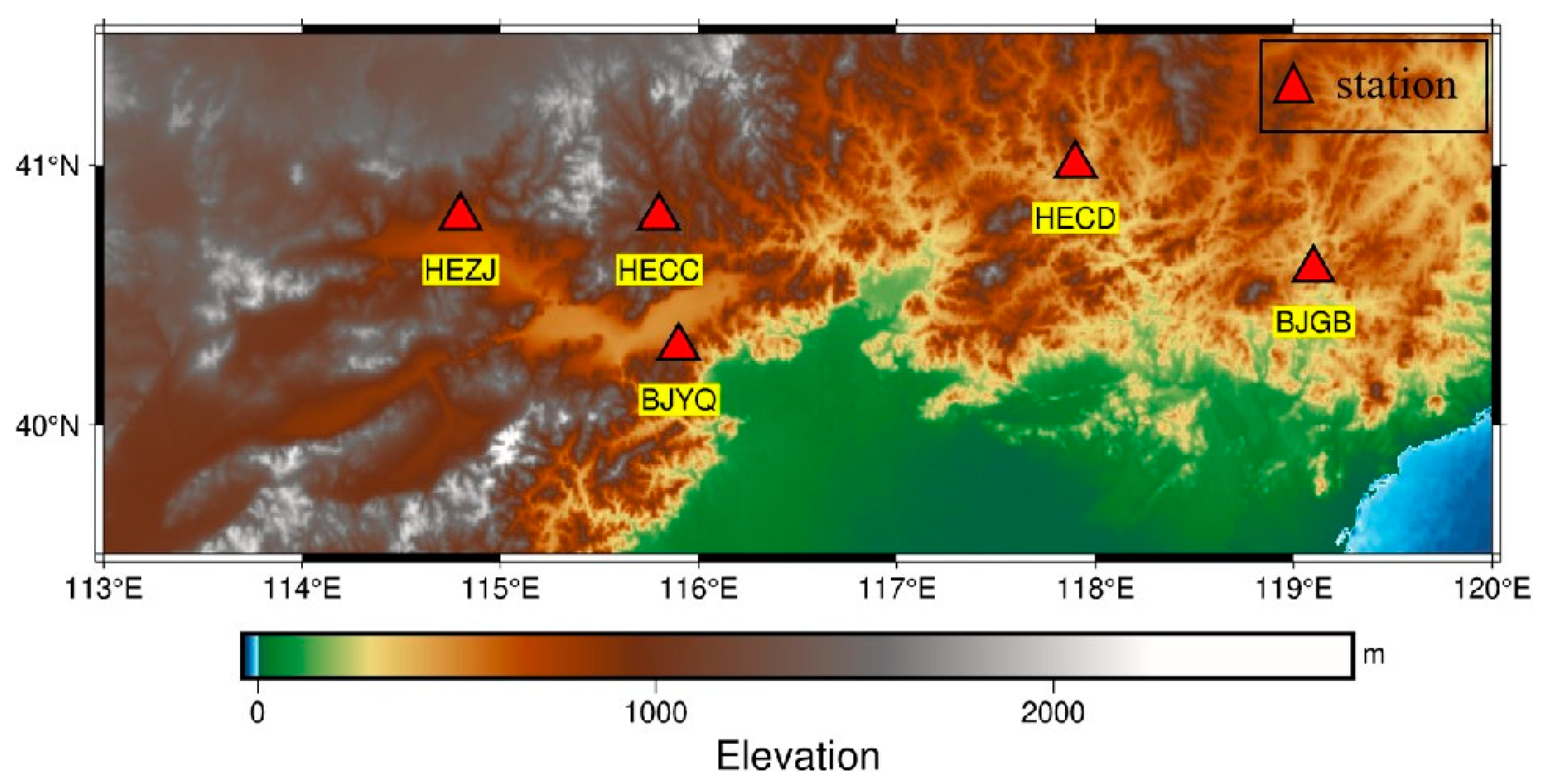
Position time series (1 January 2013–31 December 2014) of 5 GNSS reference stations located in North China are collected from the Tectonic and Environmental Observation Network of Mainland China (CMONOC II). The experimental data is provided by the China Earthquake Networks Center (
http://data.earthquake.cn, last accessed on 10 February 2021). To correctly construct the learning sample relationship in the subsequent modeling process, we mark the epochs with missing observations for the North, East, and Up (NEU) at 5 GNSS reference stations. The geographical location and information of 5 GNSS reference stations are present in
Figure 1 and
Table 1.
The nonlinear motion of GNSS reference stations is affected by environmental loading [
25,
26,
27], thermal expansion [
28,
29,
30], and tidal motions [
6,
31,
32], which make GNSS reference stations have small motion and are expressed in the GNSS position time series. Position time series among the nearby GNSS reference stations may have strong correlations due to the relevance of the geophysical effects they are subjected to [
22], so this provides the basis for modeling and interpolation of the GNSS position time series. The correlation of the vertical time series of the selected GNSS reference stations is present in
Figure 2.
2.2. Methods
The development of machine learning algorithms is of great significance for the study of a wide range of fields, such as medicine, finance, and geoscience. In particular, the classification and regression research of the decision tree-based machine learning algorithms has been widely applied and optimized. To enrich the applicable scenarios of the decision tree algorithm, researchers combine it with bagging and boosting methods to generate a series of machine learning algorithms based on the decision tree. Boosting tree algorithms are rich, among which GBDT and XGBoost algorithms have achieved excellent performances in GNSS applications [
33,
34]. The RF algorithm is a classical decision tree model optimized based on the bagging method, and its excellent operation mechanism and stability have been favored by GNSS scholars [
35]. Therefore, we hypothesize that the GBDT, XGBoost, and RF could perform well in the interpolation of the GNSS time series.
This study performs interpolation of GNSS time series by constructing a regression problem. The data set
can be expressed as:
where
represents the feature of the nth sample and is a K-dimensional vector, and
indicates the output value of the nth sample. The regression task is to construct a model
and predict the output value
based on features with minimal error.
2.2.1. GBDT Algorithm
The GBDT algorithm can be understood as an additive model consisting of
trees, which is formulated as follows:
where,
is the input sample,
is the model parameter,
is the classification and regression tree (CART),
is the weight of each tree.
and denote the loss function and the final regression tree, the GBDT algorithm is implemented as follows:
2.2.2. XGBoost Algorithm
In the XGBoost algorithm,
is defined and represented by a generalized model as:
where
is a regression tree, and
represents the score given by the kth tree to the nth observations in the data. When using function
, the following regularization objective function should be minimized as:
where
is the loss function. To prevent the model from being too complex, the penalty term
is set as:
where
is a parameter that controls the number of leaves
, and
is a parameter that controls the leaf weight
. Setting
simplifies the model generated by the algorithm and prevents overfitting.
The XGBoost algorithm minimizes the objective function via an iterative method. The objective function of the model at the jth iteration is reduced by adding the
term as
2.2.3. RF Algorithm
The base learner of the RF algorithm is CART, and the RF algorithm obtains different sample sets to construct different decision tree models by the bagging algorithm. Then the CART is pruned by using a dichotomous recursive regression technique with appropriate parameter settings, and each decision tree model is calculated to obtain the corresponding prediction value, and the final regression prediction result is the average of the prediction values of each decision tree.
For the regression problem, CART uses the minimum mean squared error (MSE) to divide the samples into 2 sample sets at the corresponding nodes of the samples and find the features and eigenvalue division points when the following two conditions are satisfied: (1) the MSE of the 2 sample sets is minimized; (2) the sum of the MSE of the 2 sample sets is minimized.
2.3. Procedure of Interpolation Experiment
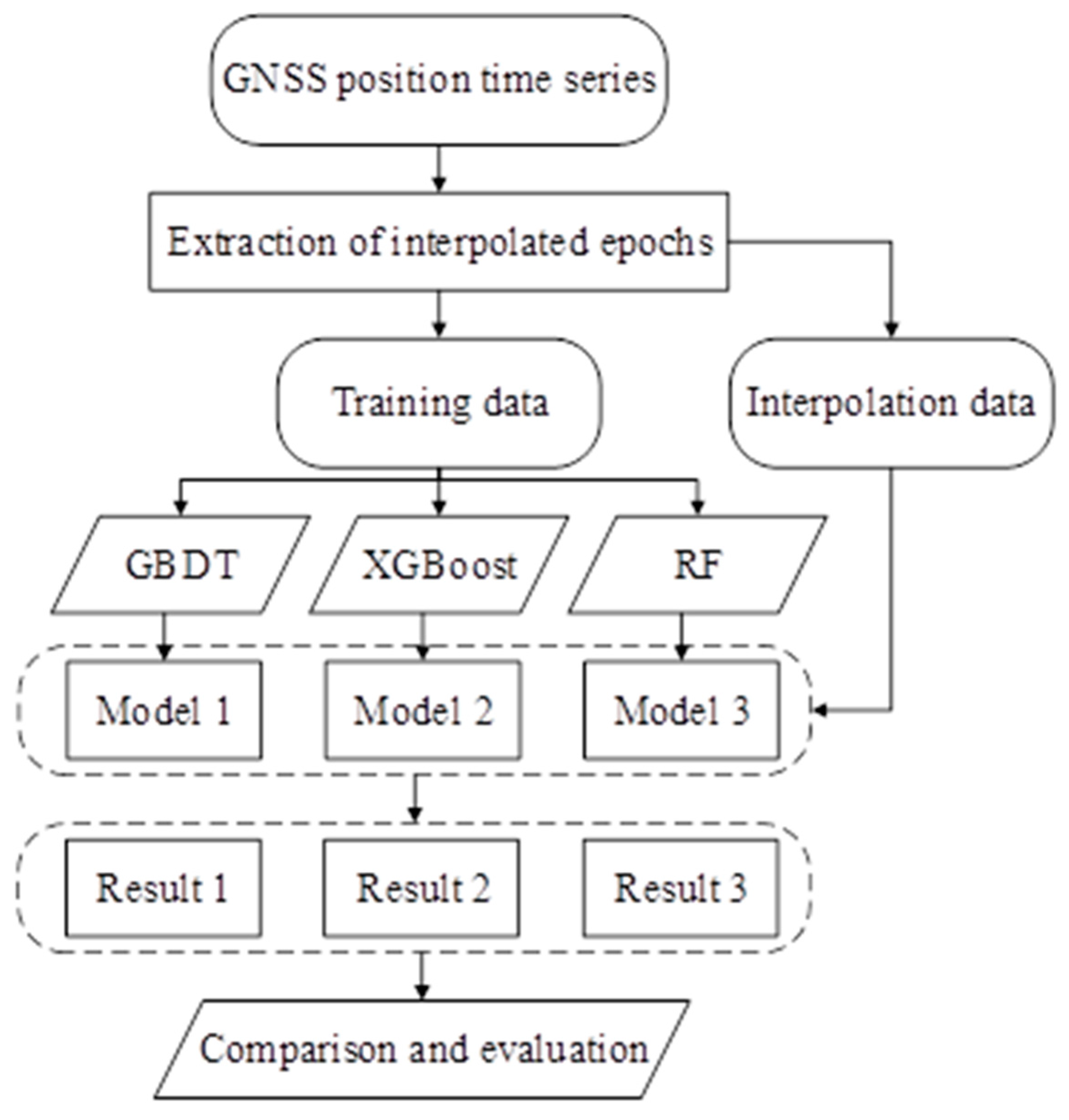
The experiment uses GBDT, XGBoost, and RF algorithms to construct regression models through correlation among GNSS reference stations to achieve interpolation of the GNSS position time series. The workflow of the experiment is presented in
Figure 3.
The main interpolation processes based on GBDT, XGBoost and, RF algorithms are described as follows:
- (1)
Extraction of the interpolated epoch. The sampling methods of interpolated epochs are mainly divided into random sampling and continuous sampling. The time series for the NEU needs to be processed separately.
- (2)
Models training. The experiment is conducted to construct regression models using GBDT, XGBoost, and RF algorithms, and the training data is input into the models for training. In this step, the target time series needs to be determined, and the time series of the remaining GNSS reference stations are used as features.
- (3)
Models output. Input the interpolation data into the trained models, and the output values of the models are the interpolated result of the corresponding epochs.
- (4)
Comparison and evaluation. Compare and evaluate the interpolated results of different models and analyze the errors.
2.4. Precision Evaluation Index
In this study, the mean absolute error (MAE) and root mean square error (RMSE) are used as the accuracy evaluation indicator of model forecasting results. MAE and RMSE can be expressed as:
where
is the original value, and
is the forecasted value. The smaller the MAE and RMSE values, the higher the forecasting accuracy of the model, and the model is more suitable for the time series.
The correlation between the forecasted time series and the original time series is determined by the Pearson correlation coefficient. The Pearson correlation coefficient considers the time series as a variable and, thus, calculates the correlation of the true and predicted time series, that is;
where
and
, respectively, represent the original time series and the forecasted time series,
and
represent the standard deviation of the original time series and the forecasted time series.
3. Results
Compared with the horizontal direction, the GNSS vertical time series has a higher noise level and more complex transient changes; thus, this section focuses on analyzing the experimental results of the GNSS vertical time series.
3.1. Interpolation of Discrete Points
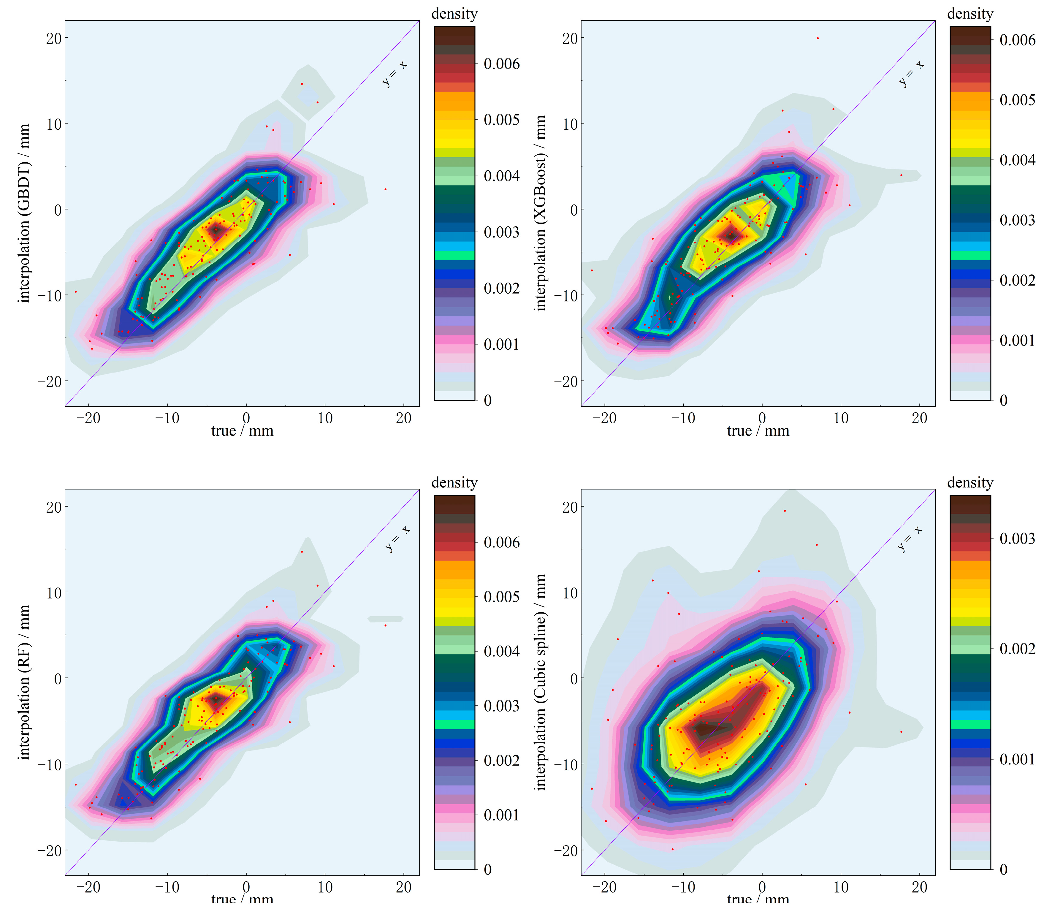
To perform interpolation of discrete points, we randomly select 5%, 10%, 15%, and 20% of the sample points as interpolation data. For better analysis of model precision, interpolation data from smaller random sampling proportions should be included in interpolation data from larger random sampling proportions. Cubic spline interpolation is a classical method that performs segmental interpolation by creating cubic equations in small intervals. To evaluate the applicability of the interpolation method in this study, we choose the cubic spline interpolation method as the comparison model. Interpolation results of discrete points (20%) at the HEZJ station are present in
Figure 4.
The red points in
Figure 4 illustrate the interpolation results of the four models for the discrete points when 20% of the sample points are randomly selected. The interpolation results of the three machine learning models are more concentrated around the purple line compared to the cubic spline interpolation model. In addition, it can be found that the error of the interpolation results of the three machine learning models is larger when the absolute value of the true value is larger. RMSE punishes the higher errors.
Table 2 compares the performance of these four models through RMSE values.
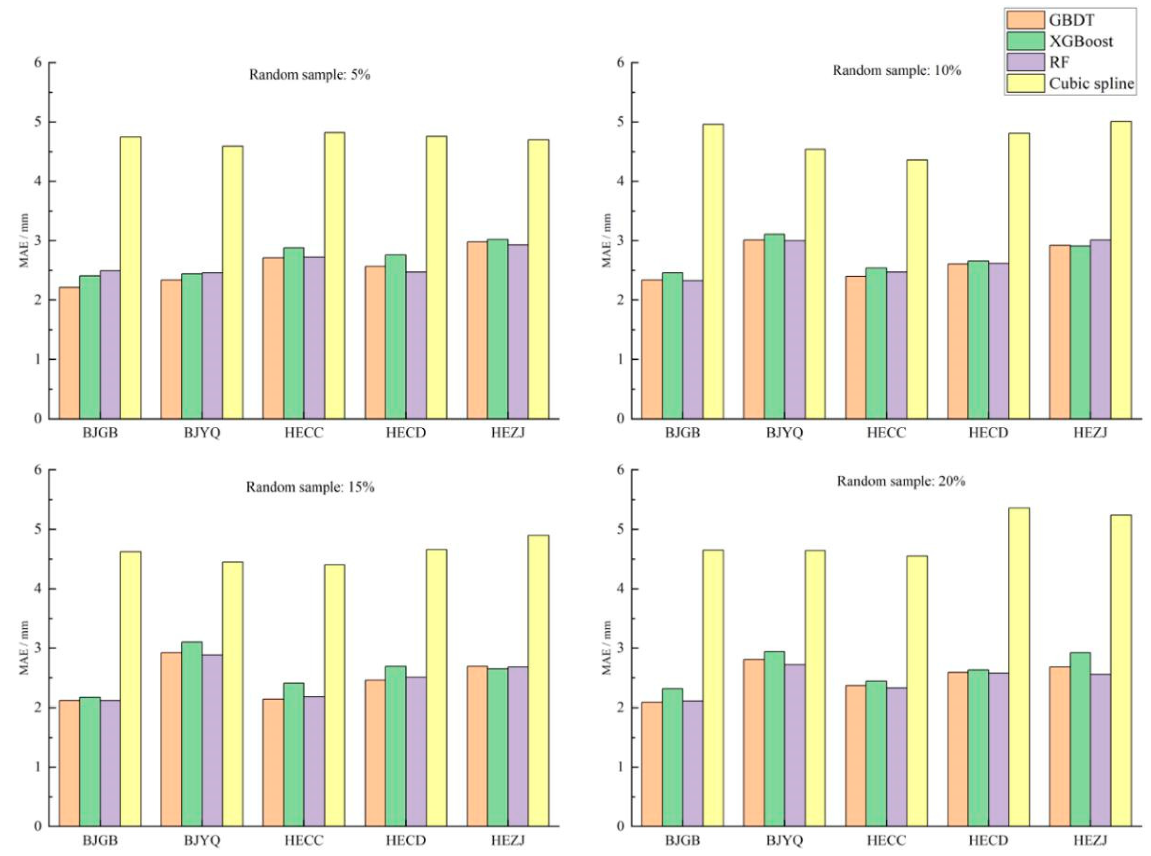
Table 2 clearly shows that the interpolation precision of the three machine learning models is more accurate and the RMSE was reduced by about 2–3 mm compared to the cubic spline interpolation model. The differences in interpolation precision of the three machine learning models were small, and the differences in MAE values were within 0.3 mm. We can also find that the interpolation precision of the three machine learning models did not decrease as the trained samples decreased, but instead presented a trend towards improved precision. The interpolation effect of the four models on random sampling data with different proportions is demonstrated in
Figure 5.
As can be seen from
Figure 5, the precision advantage of the three machine learning models was gradually evident as the proportion of missing data increased. The GBDT and RF models had better interpolation effects among the three machine learning models, and the XGBoost model had a relatively poor interpolation effect.
3.2. Interpolation of Continuous Missing Data
The experimental results in
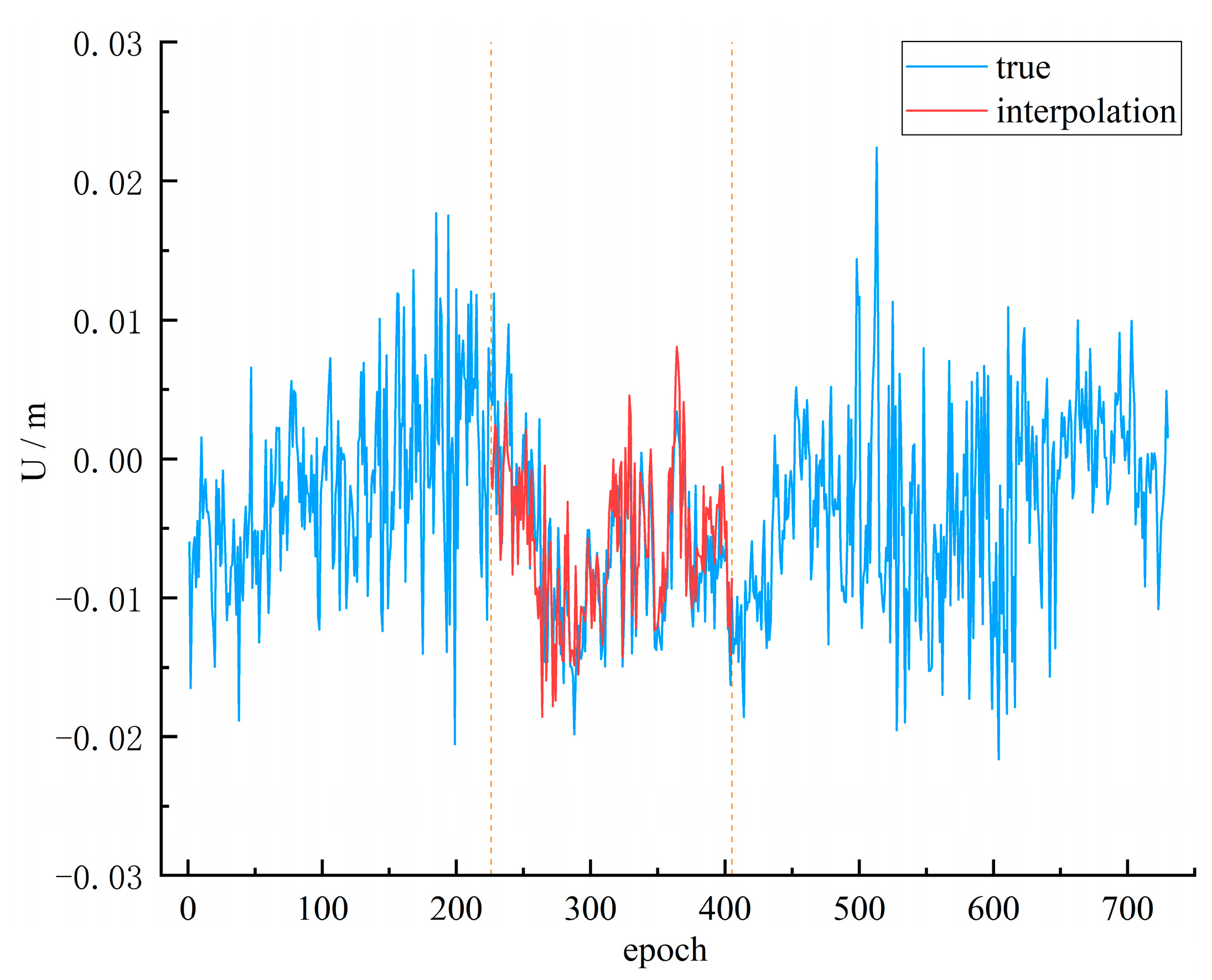
Section 3.1 show that the interpolation precision was less affected by the number of trained samples in the sampling range of 5% to 20%. Therefore, to further corroborate this phenomenon, continuous missing data will be interpolated in this section. It should be noted that increasing the number of continuous missing data required an addition to the original missing data. The interpolation results of the XGBoost model at the HEZJ station are present in
Figure 6 when data for 180 days were missing consecutively.
Figure 6 illustrates that the interpolation results of the XGBoost model maintain better consistency with the real-time series for transient changes, and the interpolation errors were mainly distributed in the initial interpolation epochs. Precision evaluation of interpolation results at 5 GNSS reference stations is given in
Table 3.
From
Table 3, it can be seen that the interpolation precision of the three machine learning models does not increase with increasing continuous missing data, which coincides with the experimental results in
Section 3.1. Except for the HECD station, the MAE of the interpolated results was the largest for three models at the remaining four GNSS reference stations when data for 30 days were consecutively missing. The relationship between interpolation precision and continuous missing data for the three models is presented in
Figure 7.
Figure 7 clearly illustrates that GBDT, XGBoost, and RF models had fine interpolation effects at all five GNSS reference stations, and the error was mainly concentrated in the first 30 days. The right part of
Figure 7 shows the relationship between the correlation coefficient and the number of missing days, illustrating that the interpolation results maintained a strong correlation with the true time series when the three machine learning models interpolate continuous missing data greater than 30 days.
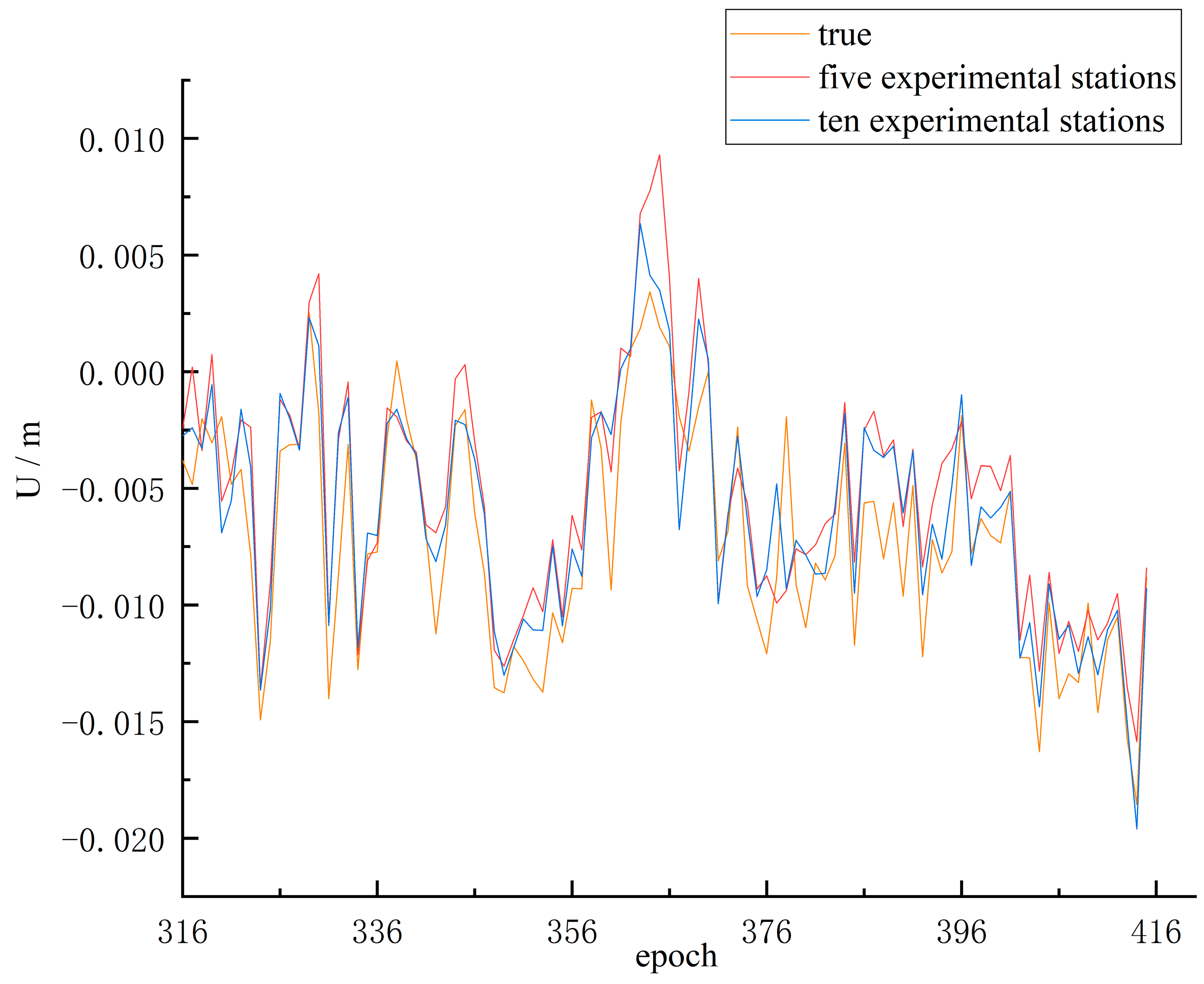
The experiments in this study use data from five GNSS reference stations as features of each other for modeling. In the modeling process of machine learning, the number and quality of features affect the precision of the model. Therefore, we added five more GNSS reference stations (BJFS, BJSH, TJBD, HELQ, and HELY stations) for the experiment, and the interpolation results of the GBDT model at the HEZJ station when the data were missing for 100 consecutive days are presented in
Figure 8.
In
Figure 8, the transient variations of the interpolation results from the two experiments were less different, and both kept excellent consistency with the real-time series, but the interpolation results were closer to the real values after increasing the number of GNSS reference stations. Precision evaluation of the interpolation results from the two experiments at the five GNSS reference stations is presented in
Table 4.
From
Table 4, it can be seen that the precision of the interpolation results was improved after adding GNSS reference stations, except for the XGBoost model, which had a small precision drop at the BJYQ station. Meanwhile, we can see that the BJGB and HEZJ stations had the more significant precision improvement, and the MAE of GBDT, XGBoost, and RF models were reduced by 25.83%, 22.17%, and 24.19% at the HEZJ station. To analyze the reasons for this phenomenon, the correlation between the vertical time series of each newly added GNSS reference station and those initial GNSS reference stations are presented in
Figure 9.
Figure 9 clearly indicates that the added GNSS reference stations have a higher correlation with the BJGB and HEZJ stations, which is the reason for the more significant improvement in the interpolation accuracy of the BJGB and HEZJ stations. Therefore, the precision improvement depends on the correlation of the added GNSS reference stations with the initial GNSS reference stations.
3.3. Interpolation of Different Seasonal Data
The experiments in
Section 3.1 and
Section 3.2 show that the interpolation precision of the three machine learning models did not decrease as the number of training samples decreased; instead, the precision was lower when the training samples were more adequate. The GNSS vertical time series had significant seasonal oscillations [
10,
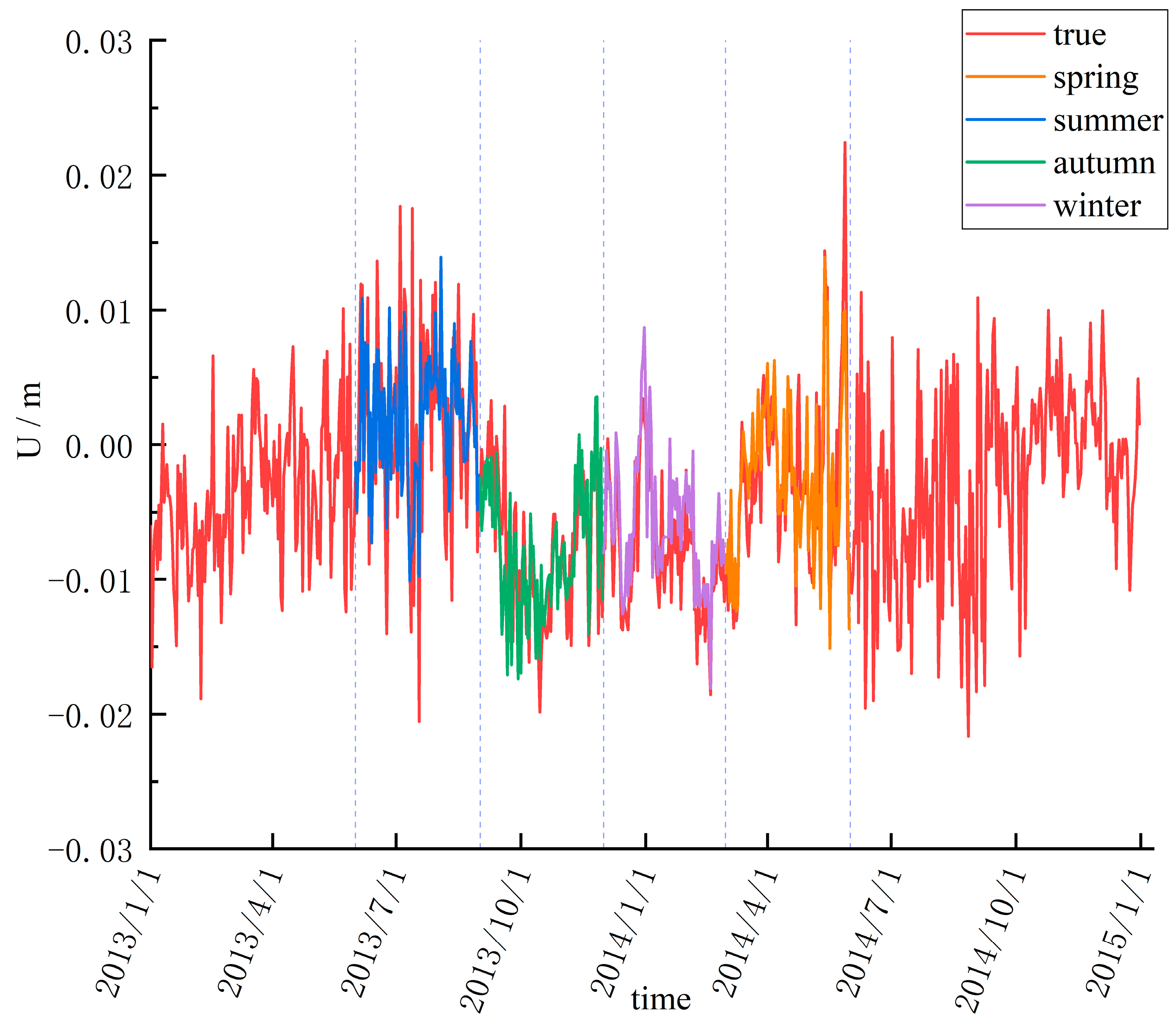
36]. Therefore, the interpolation precision may be affected by seasonal oscillations in the GNSS vertical time series. To verify this conjecture, we used machine learning methods to interpolate the different seasonal data. In the experiment, we divided data into spring (March, April, and May), summer (June, July, and August), autumn (September, October, and November), and winter (December, January, and February) parts according to months, and the interpolation results of XGBoost model at the HEZJ station are presented in
Figure 10.
We can see from
Figure 10 that there were differences in the interpolation effect for each season, with the worst interpolation effect in summer. The interpolation precision of different seasons is presented in
Table 5.
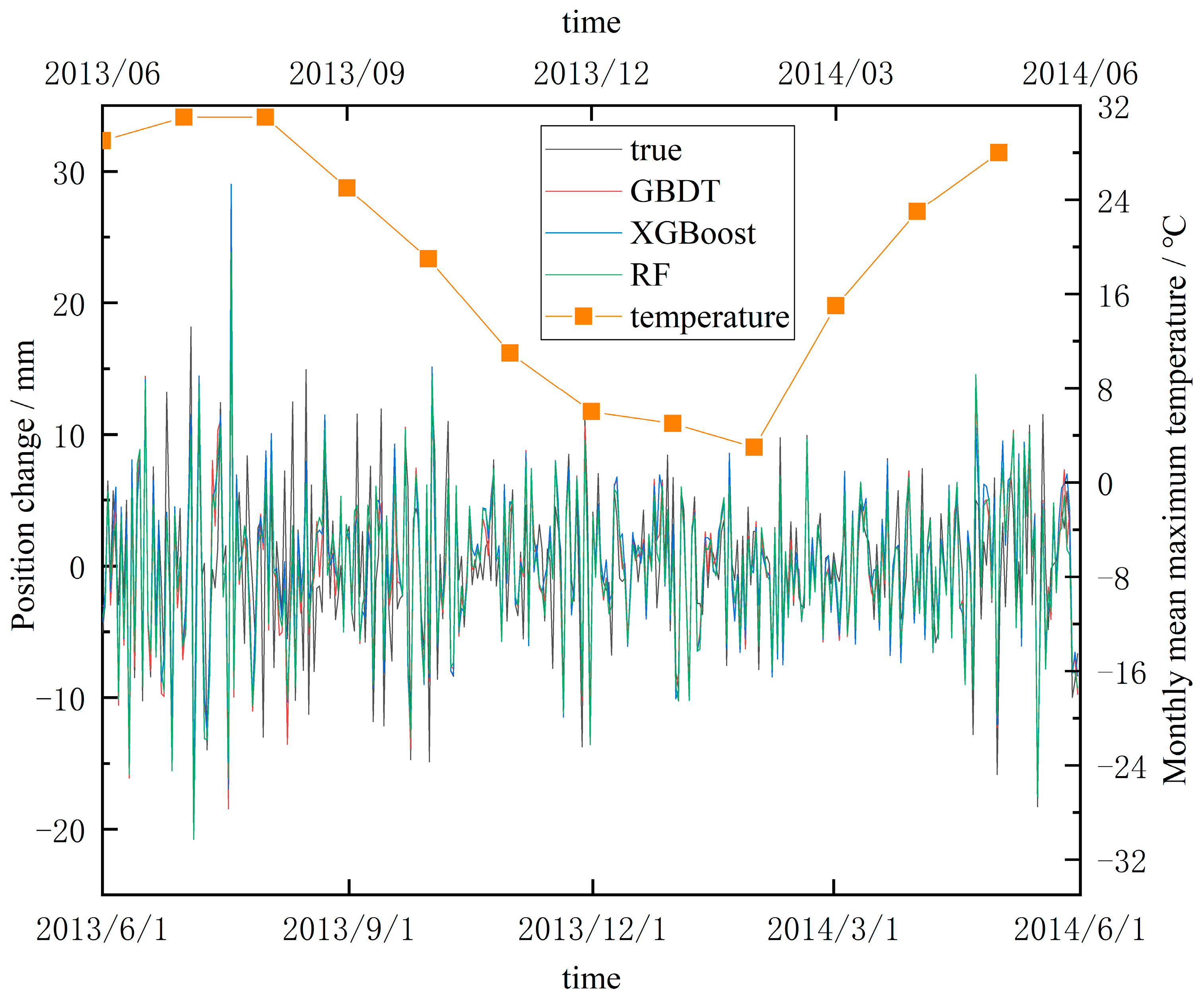
Table 5 clearly illustrates that at the five GNSS reference stations, the season with the worst interpolation precision is summer, with a 1–2 mm precision drop in MAE compared to spring and autumn, and a 2–3 mm increase in MAE compared to winter. Also, the correlation between the interpolation results and the real-time series is lower in summer compared to the remaining three seasons, which indicates that the model did not achieve good modeling effects for some transient deformations in summer. The position change of the BJGB station and the local monthly mean maximum temperature are presented in
Figure 11.
Figure 11 visually illustrates that the vertical position change oscillation amplitude at the BJGB station was positively correlated with the temperature, the seasonal oscillation amplitude at the BJGB station was larger, and the position change direction was more random in the summer when the temperature was higher. This can directly affect the interpolation precision of the GBDT, XGBoost, and RF models, resulting in poor interpolation in summer.
3.4. Interpolation of Data for the NEU
The experiments in
Section 3.1,
Section 3.2 and
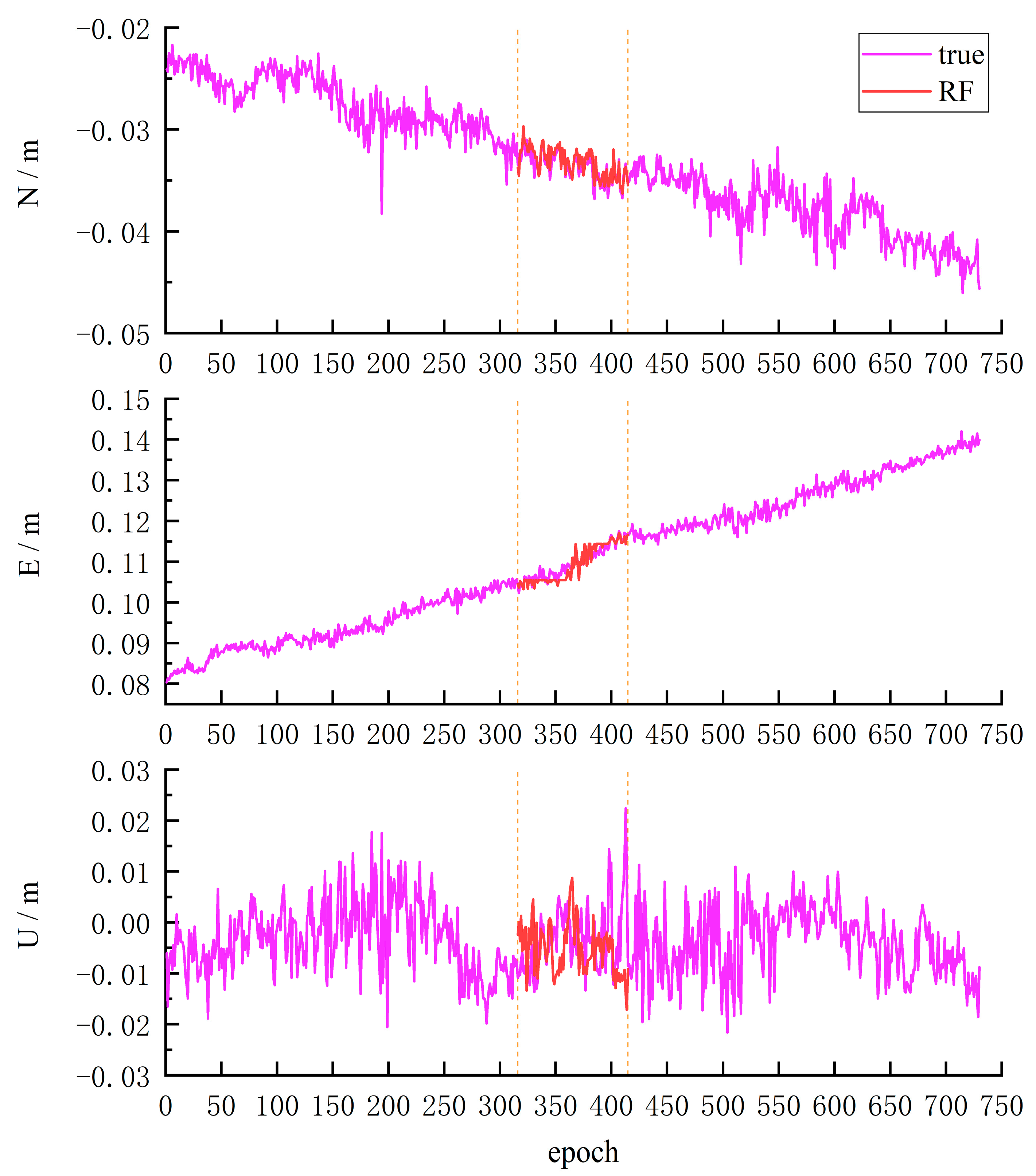
Section 3.3 all used only the GNSS vertical time series for model validation. To further evaluate the applicability of the interpolation model in this study, the interpolation effects of data for the NEU are discussed in this section. The experiment was set up with 100 days of continuous missing data, and the interpolation results of the RF model at the HEZJ station are presented in
Figure 12.
It can be seen from
Figure 12 that the RF model had the best interpolation effect on the N component, followed by the E component, and the worst interpolation effect on the U component, and there was a misjudgment of transient change in some epochs. The interpolation precision of GBDT, XGBoost, and RF models for the NEU components of the five GNSS stations is presented in
Table 6.
Table 6 shows that the difference in interpolation precision for the N component and U component between the three models was small, but compared with GBDT and RF models, the interpolation results for the E component of the XGBoost model showed a significant precision decline. We noticed that the GBDT and RF models presented consistency in the interpolation precision for the NEU components, with the best effect for the N component and the worst effect for the U component. However, the XGBoost model had the worst interpolation effect for the E component, and the MAE was about twice that of the GBDT and RF models.
Principal component analysis (PCA) was performed on the GNSS time series of the interpolated NEU components; cumulative contribution rates of the first m (m = 1, 2, 3) principal components for NEU components are presented in
Table 7.
The cumulative contribution rate of the first 1~3 principal components of the time series for the NEU components interpolated by the GBDT and RF models were higher, the retained variance was larger, and the interpolation effect was better, while the interpolation effect of the XGBoost model is the worst among the three models.
4. Discussion
Missing data in the GNSS position time series can significantly impact data processing and analysis. Therefore, accurately interpolating missing data is crucial for the GNSS position time series. High precision interpolation of non-stationary the GNSS position time series requires consideration of spatio-temporal correlation. The GBDT, XGBoost, and RF algorithms discussed in this study utilize the correlation between the GNSS position time series to construct regression problems. One key advantage of these machine learning algorithms is that they can take into account the spatio-temporal correlation among GNSS reference stations reflected in the GNSS position time series. Therefore, the regression method is more appropriate for non-stationary GNSS position time series. Moreover, compared with the traditional cubic spline interpolation method, The GBDT, XGBoost, and RF algorithms can obtain interpolation results with higher correlation. As a result, the GBDT, XGBoost, and RF algorithms are robust and efficient alternative methods for interpolation of the GNSS position time series. By analyzing the interpolation results, we also found that the model error is mainly concentrated in summer. Thus, we will try to deal with this problem by considering more physical factors (e.g., polar motion, temperature, and atmospheric pressure) in subsequent studies. In this study, the average distance between each pair of the selected GNSS reference stations is about 184 km, and the data sampling rate is 30 s, in which case we obtain highly accurate interpolation results. Therefore, We need to further examine the performance of machine learning methods and traditional methods in the interpolation of the GNSS position time series with high frequency (1 s sampling rate) in a small area (within 10 km2).
5. Conclusions
The GNSS position time series has played a fundamental role in geophysics and geodynamics studies, which has been conventionally modeled in the time domain and frequency domain over the past few decades. Taking into account the spatial correlation of GNSS reference stations, this study uses GBDT, XGBoost, and RF machine learning algorithms for modeling the GNSS time series. To form the machine learning problem, we turn the GNSS position time series to be modeled into outputs and the GNSS position time series from the remaining GNSS reference stations into input variables. The interpolation experiments of discrete points reveal that GBDT, XGBoost, and RF models always outperform the traditional cubic spline interpolation method, and the relative improvements of MAE averaged over five stations are 48.61%, 45.86%, and 49.67%, when 20% of the samples are interpolated.
Three machine learning models were then successfully used to interpolate GNSS vertical time series containing continuous missing data. Our results demonstrate that the interpolation precision of the models does not decline with increasing consecutive missing days within 180 days and maintains excellent stability. In addition, the experimental results show that the interpolation precision of the three models can be further improved by increasing the number of stations, and these added GNSS reference stations need to have a strong spatial correlation with the initial stations.
To verify whether the interpolation precision is influenced by seasonal oscillations of the GNSS vertical time series, we then perform interpolation for different seasonal data. The experimental results indicate that under the influence of temperature, the GNSS reference stations will experience larger amplitude oscillations and more random position changes in the elevation direction during summer. This phenomenon can affect the training of the three machine learning models, causing the interpolation precision of the models to decline during the summer.
Finally, we interpolate the GNSS position time series for the NEU components by the GBDT, XGBoost, and RF models. The experimental results reveal that the three models have the best interpolation effect for the N component, GBDT and RF have the worst interpolation effect for the U component, but the XGBoost model has the worst interpolation effect for the E component and appears to have a significant decrease in precision. Meanwhile, principal component analysis is performed on the interpolated time series of the five GNSS reference stations, and the analysis results show that GBDT and RF models were more suitable for interpolation of the GNSS position time series than the XGBoost model. In addition, considering the results related to different scenarios, the GBDT model is the best among the three models.
Author Contributions
Conceptualization, Z.L.; data curation, Z.L.; formal analysis, Z.L.; funding acquisition, T.L.; investigation, T.L.; methodology, Z.L.; project administration, T.L. and K.Y.; resources, T.L.; Software, Z.L.; supervision, T.L., K.Y. and J.W.; validation, Z.L.; visualization, K.Y.; writing—original draft, Z.L.; writing—review and editing, K.Y. and J.W. All authors have read and agreed to the published version of the manuscript.
Funding
This research was funded by the National Natural Science Foundation of China (42061077; 42374040), the National Natural Science Foundation of Jiangxi, China (20202BABL213033; 20202BAB212010); the Jiangxi University of Science and Technology Postgraduate Education Teaching Reform Research Project (YJG2022006), and the Hebei Water Conservancy Research Plan (2022-28).
Data Availability Statement
Not applicable.
Acknowledgments
We thank the Tectonic and Environmental Observation Network of Mainland China (CMONOC II) for providing the GNSS data. Thanks to anonymous reviewers and editors for their valuable feedback on the manuscript.
Conflicts of Interest
The authors declare no conflict of interest.
References
- Xu, X.; Sandwell, D.T.; Klein, E.; Bock, Y. Integrated Sentinel-1 InSAR and GNSS Time-Series along the San Andreas Fault System. JGR Solid Earth 2021, 126, e2021JB022579. [Google Scholar] [CrossRef]
- Xu, K.; He, R.; Li, K.; Ren, A.; Shao, Z. Secular crustal deformation characteristics prior to the 2011 Tohoku-Oki earthquake detected from GNSS array, 2003–2011. Adv. Space Res. 2022, 69, 1116–1129. [Google Scholar] [CrossRef]
- Dittmann, T.; Liu, Y.; Morton, Y.; Mencin, D. Supervised Machine Learning of High Rate GNSS Velocities for Earthquake Strong Motion Signals. JGR Solid Earth 2022, 127, e2022JB024854. [Google Scholar] [CrossRef]
- Altamimi, Z.; Collilieux, X.; Métivier, L. ITRF2008: An improved solution of the international terrestrial reference frame. J. Geod. 2011, 85, 457–473. [Google Scholar] [CrossRef]
- Altamimi, Z.; Rebischung, P.; Métivier, L.; Collilieux, X. ITRF2014: A new release of the International Terrestrial Reference Frame modeling nonlinear station motions: ITRF2014. JGR Solid Earth 2016, 121, 6109–6131. [Google Scholar] [CrossRef]
- Li, Z.; Chen, W.; Van Dam, T.; Rebischung, P.; Altamimi, Z. Comparative analysis of different atmospheric surface pressure models and their impacts on daily ITRF2014 GNSS residual time series. J. Geod. 2020, 94, 42. [Google Scholar] [CrossRef]
- Tao, Y.; Liu, C.; Liu, C.; Zhao, X.; Hu, H.; Xin, H. Joint time–frequency mask and convolutional neural network for real-time separation of multipath in GNSS deformation monitoring. GPS Solut. 2021, 25, 25. [Google Scholar] [CrossRef]
- Jiang, W.; Chen, Y.; Chen, Q.; Chen, H.; Pan, Y.; Liu, X.; Liu, T. High precision deformation monitoring with integrated GNSS and ground range observations in harsh environment. Measurement 2022, 204, 112179. [Google Scholar] [CrossRef]
- Corsa, B.; Barba-Sevilla, M.; Tiampo, K.; Meertens, C. Integration of DInSAR Time Series and GNSS Data for Continuous Volcanic Deformation Monitoring and Eruption Early Warning Applications. Remote Sens. 2022, 14, 784. [Google Scholar] [CrossRef]
- Agnieszka, W.; Dawid, K. Modeling seasonal oscillations in GNSS time series with Complementary Ensemble Empirical Mode Decomposition. GPS Solut. 2022, 26, 101. [Google Scholar] [CrossRef]
- Oelsmann, J.; Passaro, M.; Sánchez, L.; Dettmering, D.; Schwatke, C.; Seitz, F. Bayesian modelling of piecewise trends and discontinuities to improve the estimation of coastal vertical land motion: DiscoTimeS: A method to detect change points in GNSS, satellite altimetry, tide gauge and other geophysical time series. J. Geod. 2022, 96, 62. [Google Scholar] [CrossRef]
- Montillet, J.P.; Melbourne, T.I.; Szeliga, W.M. GPS Vertical Land Motion Corrections to Sea-Level Rise Estimates in the Pacific Northwest. J. Geophys. Res. Oceans 2018, 123, 1196–1212. [Google Scholar] [CrossRef]
- He, X.; Bos, M.S.; Montillet, J.P.; Fernandes, R.M.S. Investigation of the noise properties at low frequencies in long GNSS time series. J. Geod. 2019, 93, 1271–1282. [Google Scholar] [CrossRef]
- Melgar, D.; Crowell, B.W.; Melbourne, T.I.; Szeliga, W.; Santillan, M.; Scrivner, C. Noise Characteristics of Operational Real-Time High-Rate GNSS Positions in a Large Aperture Network. JGR Solid Earth 2020, 125, e2019JB019197. [Google Scholar] [CrossRef]
- Benoist, C.; Collilieux, X.; Rebischung, P.; Altamimi, Z.; Jamet, O.; Métivier, L.; Chanard, K.; Bel, L. Accounting for spatiotemporal correlations of GNSS coordinate time series to estimate station velocities. J. Geodyn. 2020, 135, 101693. [Google Scholar] [CrossRef]
- Wang, X.; Cheng, Y.; Wu, S.; Zhang, K. An effective toolkit for the interpolation and gross error detection of GPS time series. Surv. Rev. 2016, 48, 202–211. [Google Scholar] [CrossRef]
- Liu, N.; Dai, W.; Santerre, R.; Kuang, C. A MATLAB-based Kriged Kalman Filter software for interpolating missing data in GNSS coordinate time series. GPS Solut. 2018, 22, 25. [Google Scholar] [CrossRef]
- Zhang, S.; Gong, L.; Zeng, Q.; Li, W.; Xiao, F.; Lei, J. Imputation of GPS Coordinate Time Series Using missForest. Remote Sens. 2021, 13, 2312. [Google Scholar] [CrossRef]
- Bao, Z.; Chang, G.; Zhang, L.; Chen, G.; Zhang, S. Filling missing values of multi-station GNSS coordinate time series based on matrix completion. Measurement 2021, 183, 109862. [Google Scholar] [CrossRef]
- Qiu, X.; Wang, F.; Zhou, Y.; Zhou, S. Iteration empirical mode decomposition method for filling the missing data of GNSS position time series. Acta Geodyn. Geomater. 2022, 19, 271–279. [Google Scholar] [CrossRef]
- Gao, W.; Li, Z.; Chen, Q.; Jiang, W.; Feng, Y. Modelling and prediction of GNSS time series using GBDT, LSTM and SVM machine learning approaches. J. Geod. 2022, 96, 71. [Google Scholar] [CrossRef]
- Li, Z.; Lu, T.; He, X.; Montillet, J.P.; Tao, R. An improved cyclic multi model-eXtreme gradient boosting (CMM-XGBoost) forecasting algorithm on the GNSS vertical time series. Adv. Space Res. 2023, 71, 912–935. [Google Scholar] [CrossRef]
- Jia, Y.; Jin, S.; Savi, P.; Yan, Q.; Li, W. Modeling and Theoretical Analysis of GNSS-R Soil Moisture Retrieval Based on the Random Forest and Support Vector Machine Learning Approach. Remote Sens. 2020, 12, 3679. [Google Scholar] [CrossRef]
- Niu, Y.; Rebischung, P.; Li, M.; Wei, N.; Shi, C.; Altamimi, Z. Temporal spectrum of spatial correlations between GNSS station position time series. J. Geod. 2023, 97, 12. [Google Scholar] [CrossRef]
- Deng, L.; Jiang, W.; Li, Z.; Chen, H.; Wang, K.; Ma, Y. Assessment of second- and third-order ionospheric effects on regional networks: Case study in China with longer CMONOC GPS coordinate time series. J. Geod. 2017, 91, 207–227. [Google Scholar] [CrossRef]
- Materna, K.; Feng, L.; Lindsey, E.O.; Hill, E.M.; Ahsan, A.; Alam, A.K.M.K.; Oo, K.M.; Than, O.; Aung, T.; Khaing, S.N.; et al. GNSS characterization of hydrological loading in South and Southeast Asia. Geophys. J. Int. 2020, 224, 1742–1752. [Google Scholar] [CrossRef]
- He, Y.; Nie, G.; Wu, S.; Li, H. Comparative analysis of the correction effect of different environmental loading products on global GNSS coordinate time series. Adv. Space Res. 2022, 70, 3594–3613. [Google Scholar] [CrossRef]
- Zhu, Z.; Zhou, X.; Deng, L.; Wang, K.; Zhou, B. Quantitative analysis of geophysical sources of common mode component in CMONOC GPS coordinate time series. Adv. Space Res. 2017, 60, 2896–2909. [Google Scholar] [CrossRef]
- Wang, K.; Jiang, W.; Chen, H.; An, X.; Zhou, X.; Yuan, P.; Chen, Q. Analysis of Seasonal Signal in GPS Short-Baseline Time Series. Pure Appl. Geophys. 2018, 175, 3485–3509. [Google Scholar] [CrossRef]
- Liu, B.; Ma, X.; Xing, X.; Tan, J.; Peng, W.; Zhang, L. Quantitative Evaluation of Environmental Loading Products and Thermal Expansion Effect for Correcting GNSS Vertical Coordinate Time Series in Taiwan. Remote Sens. 2022, 14, 4480. [Google Scholar] [CrossRef]
- Chanard, K.; Fleitout, L.; Calais, E.; Rebischung, P.; Avouac, J. Toward a Global Horizontal and Vertical Elastic Load Deformation Model Derived from GRACE and GNSS Station Position Time Series. JGR Solid Earth 2018, 123, 3225–3237. [Google Scholar] [CrossRef]
- Martens, H.R.; Argus, D.F.; Norberg, C.; Blewitt, G.; Herring, T.A.; Moore, A.W.; Hammond, W.C.; Kreemer, C. Atmospheric pressure loading in GPS positions: Dependency on GPS processing methods and effect on assessment of seasonal deformation in the contiguous USA and Alaska. J. Geod. 2020, 94, 115. [Google Scholar] [CrossRef]
- Zheng, Y.; Lu, C.; Wu, Z.; Liao, J.; Zhang, Y.; Wang, Q. Machine Learning-Based Model for Real-Time GNSS Precipitable Water Vapor Sensing. Geophys. Res. Lett. 2022, 49, e2021GL096408. [Google Scholar] [CrossRef]
- Jia, Y.; Jin, S.; Savi, P.; Gao, Y.; Tang, J.; Chen, Y.; Li, W. GNSS-R Soil Moisture Retrieval Based on a XGboost Machine Learning Aided Method: Performance and Validation. Remote Sens. 2019, 11, 1655. [Google Scholar] [CrossRef]
- Altuntas, C.; Iban, M.C.; Şentürk, E.; Durdag, U.M.; Tunalioglu, N. Machine learning-based snow depth retrieval using GNSS signal-to-noise ratio data. GPS Solut. 2022, 26, 117. [Google Scholar] [CrossRef]
- Yan, J.; Dong, D.; Bürgmann, R.; Materna, K.; Tan, W.; Peng, Y.; Chen, J. Separation of Sources of Seasonal Uplift in China Using Independent Component Analysis of GNSS Time Series. JGR Solid Earth 2019, 124, 11951–11971. [Google Scholar] [CrossRef]
Figure 1.
The geographical location of five GNSS reference stations in North China.
Figure 1.
The geographical location of five GNSS reference stations in North China.
Figure 2.
The correlation of the vertical time series of GNSS reference stations.
Figure 2.
The correlation of the vertical time series of GNSS reference stations.
Figure 3.
Workflow of study case of interpolation.
Figure 3.
Workflow of study case of interpolation.
Figure 4.
Interpolation results of discrete points (20%) at the HEZJ station.
Figure 4.
Interpolation results of discrete points (20%) at the HEZJ station.
Figure 5.
Interpolation effect of different models on random sampling data.
Figure 5.
Interpolation effect of different models on random sampling data.
Figure 6.
Interpolation results of the XGBoost model at HEZJ station (180 days).
Figure 6.
Interpolation results of the XGBoost model at HEZJ station (180 days).
Figure 7.
Interpolation effect of different models on continuous missing data.
Figure 7.
Interpolation effect of different models on continuous missing data.
Figure 8.
Interpolation results of the GBDT model at the HEZJ station.
Figure 8.
Interpolation results of the GBDT model at the HEZJ station.
Figure 9.
Correlation of elevation time series between stations.
Figure 9.
Correlation of elevation time series between stations.
Figure 10.
Interpolation results of XGBoost model for different seasonal data at the HEZJ station.
Figure 10.
Interpolation results of XGBoost model for different seasonal data at the HEZJ station.
Figure 11.
Position change and monthly mean maximum temperature of the BJGB station.
Figure 11.
Position change and monthly mean maximum temperature of the BJGB station.
Figure 12.
Interpolation results of RF model at the HEZJ station.
Figure 12.
Interpolation results of RF model at the HEZJ station.
Table 1.
The information of five GNSS reference stations in North China.
Table 1.
The information of five GNSS reference stations in North China.
| Station | Longitude | Latitude | Characteristic | Establishment Time | Sampling Rate | Average Distance |
|---|
| BJGB | 119.1°E | 40.6°N | soil layer | 2009 | 30 s | 256.3 km |
| BJYQ | 115.9°E | 40.3°N | bedrock | 2009 | 30 s | 155.8 km |
| HECC | 115.8°E | 40.8°N | bedrock | 2009 | 30 s | 134.3 km |
| HECD | 117.9°E | 41.0°N | bedrock | 2009 | 30 s | 168.8 km |
| HEZJ | 114.8°E | 40.8°N | bedrock | 2009 | 30 s | 204.2 km |
Table 2.
The RMSE (mm) of the interpolation results of the discrete points.
Table 2.
The RMSE (mm) of the interpolation results of the discrete points.
| Station | Missing Rate | GBDT | XGBoost | RF | Cubic Spline |
|---|
| BJGB | 5% | 2.97 | 3.02 | 3.29 | 6.33 |
| 10% | 3.03 | 3.12 | 3.02 | 6.95 |
| 15% | 2.74 | 2.17 | 2.75 | 6.53 |
| 20% | 2.84 | 2.86 | 2.83 | 6.74 |
| BJYQ | 5% | 3.37 | 3.39 | 3.41 | 6.53 |
| 10% | 4.25 | 4.59 | 4.28 | 5.90 |
| 15% | 4.52 | 4.81 | 4.33 | 6.11 |
| 20% | 4.33 | 4.58 | 4.10 | 6.63 |
| HECC | 5% | 3.49 | 3.82 | 3.63 | 6.73 |
| 10% | 3.22 | 3.46 | 3.37 | 6.24 |
| 15% | 2.91 | 3.25 | 2.97 | 6.20 |
| 20% | 3.27 | 3.34 | 3.23 | 6.88 |
| HECD | 5% | 3.06 | 3.24 | 3.02 | 6.80 |
| 10% | 3.13 | 3.33 | 3.25 | 6.80 |
| 15% | 3.09 | 3.33 | 3.22 | 6.58 |
| 20% | 3.61 | 3.60 | 3.57 | 7.71 |
| HEZJ | 5% | 4.05 | 4.51 | 3.84 | 6.49 |
| 10% | 3.96 | 4.28 | 3.89 | 7.05 |
| 15% | 3.71 | 3.80 | 3.51 | 6.81 |
| 20% | 3.69 | 4.01 | 3.41 | 7.31 |
Table 3.
Precision evaluation of interpolation results for three machine learning.
Table 3.
Precision evaluation of interpolation results for three machine learning.
| Station | Missing Days | GBDT | XGBoost | RF |
|---|
| MAE/mm | | MAE/mm | | MAE/mm | |
|---|
| BJGB | 30 | 4.13 | 0.33 | 4.33 | 0.23 | 4.21 | 0.34 |
| 60 | 3.35 | 0.79 | 3.34 | 0.79 | 3.58 | 0.77 |
| 120 | 2.63 | 0.83 | 2.81 | 0.82 | 2.69 | 0.83 |
| 180 | 2.26 | 0.85 | 2.40 | 0.85 | 2.34 | 0.85 |
| BJYQ | 30 | 3.37 | 0.42 | 3.19 | 0.39 | 3.36 | 0.48 |
| 60 | 3.07 | 0.77 | 3.30 | 0.77 | 3.36 | 0.78 |
| 120 | 2.54 | 0.82 | 2.96 | 0.78 | 2.76 | 0.82 |
| 180 | 2.47 | 0.84 | 2.61 | 0.82 | 2.48 | 0.84 |
| HECC | 30 | 3.71 | 0.36 | 3.91 | 0.33 | 4.01 | 0.32 |
| 60 | 2.65 | 0.84 | 3.18 | 0.81 | 2.95 | 0.80 |
| 120 | 2.27 | 0.87 | 2.44 | 0.84 | 2.39 | 0.85 |
| 180 | 2.15 | 0.87 | 2.28 | 0.86 | 2.18 | 0.87 |
| HECD | 30 | 2.70 | 0.65 | 2.76 | 0.61 | 3.12 | 0.48 |
| 60 | 3.51 | 0.87 | 3.54 | 0.87 | 3.43 | 0.88 |
| 120 | 2.74 | 0.86 | 2.93 | 0.84 | 2.68 | 0.87 |
| 180 | 2.51 | 0.85 | 2.56 | 0.85 | 2.51 | 0.86 |
| HEZJ | 30 | 3.67 | 0.75 | 2.86 | 0.67 | 3.45 | 0.69 |
| 60 | 3.60 | 0.80 | 3.11 | 0.80 | 3.46 | 0.81 |
| 120 | 2.77 | 0.81 | 2.85 | 0.81 | 2.70 | 0.83 |
| 180 | 2.69 | 0.80 | 2.78 | 0.78 | 2.62 | 0.82 |
Table 4.
Precision evaluation of interpolation results before and after adding GNSS stations.
Table 4.
Precision evaluation of interpolation results before and after adding GNSS stations.
| Station | Experimental Stations | GBDT | XGBoost | RF |
|---|
| MAE/mm | | MAE/mm | | MAE/mm | |
|---|
| BJGB | 5 | 1.62 | 0.91 | 1.72 | 0.90 | 1.55 | 0.92 |
| 10 | 1.39 | 0.94 | 1.46 | 0.93 | 1.38 | 0.94 |
| BJYQ | 5 | 2.18 | 0.88 | 2.11 | 0.89 | 2.00 | 0.89 |
| 10 | 1.98 | 0.89 | 2.16 | 0.87 | 1.91 | 0.90 |
| HECC | 5 | 1.89 | 0.91 | 1.77 | 0.90 | 1.78 | 0.91 |
| 10 | 1.75 | 0.92 | 1.74 | 0.90 | 1.68 | 0.93 |
| HECD | 5 | 1.73 | 0.90 | 1.82 | 0.89 | 1.83 | 0.89 |
| 10 | 1.60 | 0.92 | 1.66 | 0.90 | 1.50 | 0.93 |
| HEZJ | 5 | 2.40 | 0.90 | 2.48 | 0.90 | 2.48 | 0.89 |
| 10 | 1.78 | 0.91 | 1.93 | 0.91 | 1.88 | 0.91 |
Table 5.
Interpolation precision of the five GNSS reference stations in different seasons.
Table 5.
Interpolation precision of the five GNSS reference stations in different seasons.
| Station | Missing Season | GBDT | XGBoost | RF |
|---|
| MAE/mm | | MAE/mm | | MAE/mm | |
|---|
| BJGB | spring | 2.24 | 0.87 | 2.30 | 0.88 | 2.17 | 0.87 |
| summer | 3.65 | 0.68 | 3.28 | 0.69 | 3.57 | 0.67 |
| autumn | 2.54 | 0.82 | 2.73 | 0.80 | 2.65 | 0.81 |
| winter | 1.46 | 0.92 | 1.61 | 0.90 | 1.42 | 0.93 |
| BJYQ | spring | 2.69 | 0.82 | 2.79 | 0.81 | 2.71 | 0.82 |
| summer | 4.18 | 0.57 | 4.10 | 0.61 | 3.69 | 0.67 |
| autumn | 2.34 | 0.81 | 2.58 | 0.83 | 2.56 | 0.81 |
| winter | 2.10 | 0.89 | 2.03 | 0.90 | 1.87 | 0.91 |
| HECC | spring | 2.42 | 0.87 | 2.31 | 0.88 | 2.48 | 0.86 |
| summer | 3.79 | 0.74 | 3.84 | 0.74 | 3.94 | 0.73 |
| autumn | 2.12 | 0.87 | 2.37 | 0.85 | 2.11 | 0.86 |
| winter | 1.79 | 0.92 | 1.68 | 0.91 | 1.86 | 0.91 |
| HECD | spring | 2.41 | 0.84 | 2.48 | 0.85 | 2.45 | 0.84 |
| summer | 4.43 | 0.63 | 4.34 | 0.63 | 4.04 | 0.67 |
| autumn | 2.83 | 0.82 | 2.92 | 0.83 | 2.73 | 0.86 |
| winter | 1.76 | 0.89 | 1.81 | 0.88 | 1.82 | 0.88 |
| HEZJ | spring | 2.71 | 0.85 | 2.80 | 0.84 | 2.94 | 0.82 |
| summer | 4.69 | 0.64 | 3.78 | 0.66 | 4.63 | 0.66 |
| autumn | 2.66 | 0.76 | 2.88 | 0.75 | 2.72 | 0.78 |
| winter | 2.42 | 0.89 | 2.39 | 0.89 | 2.36 | 0.90 |
Table 6.
Precision evaluation of interpolation results for the NEU components.
Table 6.
Precision evaluation of interpolation results for the NEU components.
| Station | Direction | GBDT | XGBoost | RF |
|---|
| MAE/mm | | MAE/mm | | MAE/mm | |
|---|
| BJGB | N | 0.75 | 0.83 | 0.81 | 0.76 | 0.78 | 0.82 |
| E | 1.22 | 0.93 | 2.30 | 0.84 | 1.16 | 0.93 |
| U | 1.62 | 0.91 | 1.72 | 0.90 | 1.55 | 0.92 |
| BJYQ | N | 0.65 | 0.81 | 0.78 | 0.75 | 0.62 | 0.81 |
| E | 1.37 | 0.92 | 2.46 | 0.83 | 1.22 | 0.93 |
| U | 2.18 | 0.88 | 2.11 | 0.89 | 2.00 | 0.89 |
| HECC | N | 0.76 | 0.79 | 1.03 | 0.66 | 0.75 | 0.83 |
| E | 1.10 | 0.92 | 2.24 | 0.84 | 1.08 | 0.94 |
| U | 1.89 | 0.91 | 1.77 | 0.90 | 1.78 | 0.91 |
| HECD | N | 0.53 | 0.85 | 0.69 | 0.79 | 0.49 | 0.87 |
| E | 1.09 | 0.94 | 2.21 | 0.84 | 1.12 | 0.94 |
| U | 1.73 | 0.90 | 1.82 | 0.89 | 1.83 | 0.89 |
| HEZJ | N | 0.59 | 0.88 | 0.75 | 0.82 | 0.59 | 0.89 |
| E | 1.43 | 0.92 | 2.15 | 0.85 | 1.29 | 0.94 |
| U | 2.40 | 0.90 | 2.48 | 0.90 | 2.48 | 0.89 |
Table 7.
Cumulative contribution rate of principal components for different interpolation models.
Table 7.
Cumulative contribution rate of principal components for different interpolation models.
| Component | Interpolation Model | Cumulative Contribution Rate |
|---|
| m = 1 | m = 2 | m = 3 |
|---|
| N | GBDT | 93.67% | 96.71% | 98.69% |
| XGBoost | 87.11% | 93.97% | 96.96% |
| RF | 93.87% | 96.51% | 98.12% |
| E | GBDT | 97.54% | 98.87% | 99.48% |
| XGBoost | 94.03% | 99.82% | 99.90% |
| RF | 99.28% | 99.58% | 99.77% |
| U | GBDT | 96.04% | 97.53% | 98.65% |
| XGBoost | 94.77% | 96.47% | 97.89% |
| RF | 95.57% | 97.25% | 98.49% |
| Disclaimer/Publisher’s Note: The statements, opinions and data contained in all publications are solely those of the individual author(s) and contributor(s) and not of MDPI and/or the editor(s). MDPI and/or the editor(s) disclaim responsibility for any injury to people or property resulting from any ideas, methods, instructions or products referred to in the content. |
© 2023 by the authors. Licensee MDPI, Basel, Switzerland. This article is an open access article distributed under the terms and conditions of the Creative Commons Attribution (CC BY) license (https://creativecommons.org/licenses/by/4.0/).
