Article

Decentralized Approach for Translational Motion Estimation with Multistatic Inverse Synthetic Aperture Radar Systems

Department of Information Engineering, Electronics and Telecommunications DIET, Sapienza University of Rome, Via Eudossiana, 18, 00184 Rome, Italy
*
Author to whom correspondence should be addressed.
Remote Sens. 2023, 15(18), 4372; https://doi.org/10.3390/rs15184372
Submission received: 17 July 2023 / Revised: 30 August 2023 / Accepted: 2 September 2023 / Published: 5 September 2023
(This article belongs to the Special Issue Advanced Radar Signal Processing and Applications)

Abstract

:
This paper addresses the estimation of the target translational motion by using a multistatic Inverse Synthetic Aperture Radar (ISAR) system composed of an active radar sensor and multiple receiving-only devices. Particularly, a two-step decentralized technique is derived: the first step estimates specific signal parameters (i.e., Doppler frequency and Doppler rate) at the single-sensor level, while the second step exploits these estimated parameters to derive the target velocity and acceleration components. Specifically, the second step is organized in two stages: the former is for velocity estimation, while the latter is devoted to velocity estimation refinement if a constant velocity model motion can be regarded as acceptable, or to acceleration estimation if a constant velocity assumption does not apply. A proper decision criterion to select between the two motion models is also provided. A closed-form theoretical performance analysis is provided for the overall technique, which is then used to assess the achievable performance under different distributions of the radar sensors. Additionally, a comparison with a state-of-the-art centralized approach has been carried out considering computational burden and robustness. Finally, results obtained against experimental multisensory data are shown confirming the effectiveness of the proposed technique and supporting its practical application.

1. Introduction

As well known, radar images of man-made targets can be obtained by means of Inverse Synthetic Aperture Radar (ISAR) techniques, [1,2]. Compared to other methods, ISAR imaging has the advantage of generating all-day, all-weather maps of target reflectivity. This strength makes it an important system for target classification and recognition applications.
Nevertheless, conventional (i.e., single channel and single sensor) ISAR systems show the following inherent drawbacks: ( i ) conventional ISAR images provide a two-dimensional projection of targets having a 3D structure; ( ii ) achievable cross-range resolution depends on the intrinsic characteristics of the target motion and therefore, depending on the specific conditions, can be very poor; and ( iii ) the formation of an ISAR image requires the knowledge of the target motion parameters (both translation and rotation). Since generally, the targets are non-cooperative, these parameters must be estimated directly from the received signal.
Regarding the 3D target reconstruction, point ( i ), interferometric ISAR (InISAR) systems offer a solution by applying interferometric technology to the ISAR images of multi-antenna systems. The traditional InISAR imaging usually employs three antennas to construct two perpendicular baselines [3]. However, in practical applications, it is not a simple matter to guarantee the complete orthogonality of the baselines due to the existence of factors such as system errors or environmental constraints. In [4], a practical maneuvering target 3D imaging algorithm based on the InISAR of an arbitrary three-antenna configuration is investigated.
The use of multistatic, or even Multiple Input Multiple Output (MIMO), ISAR systems with multiple sensors observing the same target with different acquisitions geometries and the joint exploitation of the acquired data allow much richer information to be garnered, overcoming limitations (ii) and (iii) imposed by conventional systems due to their single perspective. Over the last decade, researchers investigated the potentialities of multistatic/MIMO ISAR configurations for different tasks, see [5] and references therein.
In particular, distributed ISAR techniques have been also proposed to address the issues specified in ( ii ) . For example, to enhance the cross-range resolution of rotating targets, multiple transmitters-receivers can synthesize a wider observation angle than the single sensor, bringing to a higher resolution [6,7,8]. Such approaches rely on a proper coherent combination of the received signals and, therefore, are effective in the case of limited angular separations among the individual sensors so that a stable behavior of the scattering mechanism can be assumed. In the case of a wider separation among the sensors, such an assumption does not hold. As the target e.m. response varies when observed by significantly different observation angles, incoherent combination approaches must be considered (e.g., [9] shows that enhanced target classification can be obtained by incoherent summation of single-sensor images acquired by spatially distributed sensors).
Finally, point ( iii ) , even if motion compensation and image scaling are possible also with a conventional single sensor (limitations may be present for scaling), multistatic systems can be exploited for an enhanced estimation of the motion of the target. Specifically, in this respect, the main advantage of the multistatic systems compared to the monostatic (conventional single sensor) ones is the possibility to recover the complete target motion, namely:
  • Velocity and acceleration ( x ,   y ) components for translation motion while in contrast, at the most, a single sensor could allow us to estimate the radial velocity and the modulus of the cross-range velocity (i.e., indeterminate sign).
  • Roll, pitch, and yaw rates for rotation motion while only the overall effective rotation rate, or at the most, the vertical and horizontal rotation components could be estimated by single-sensor techniques.
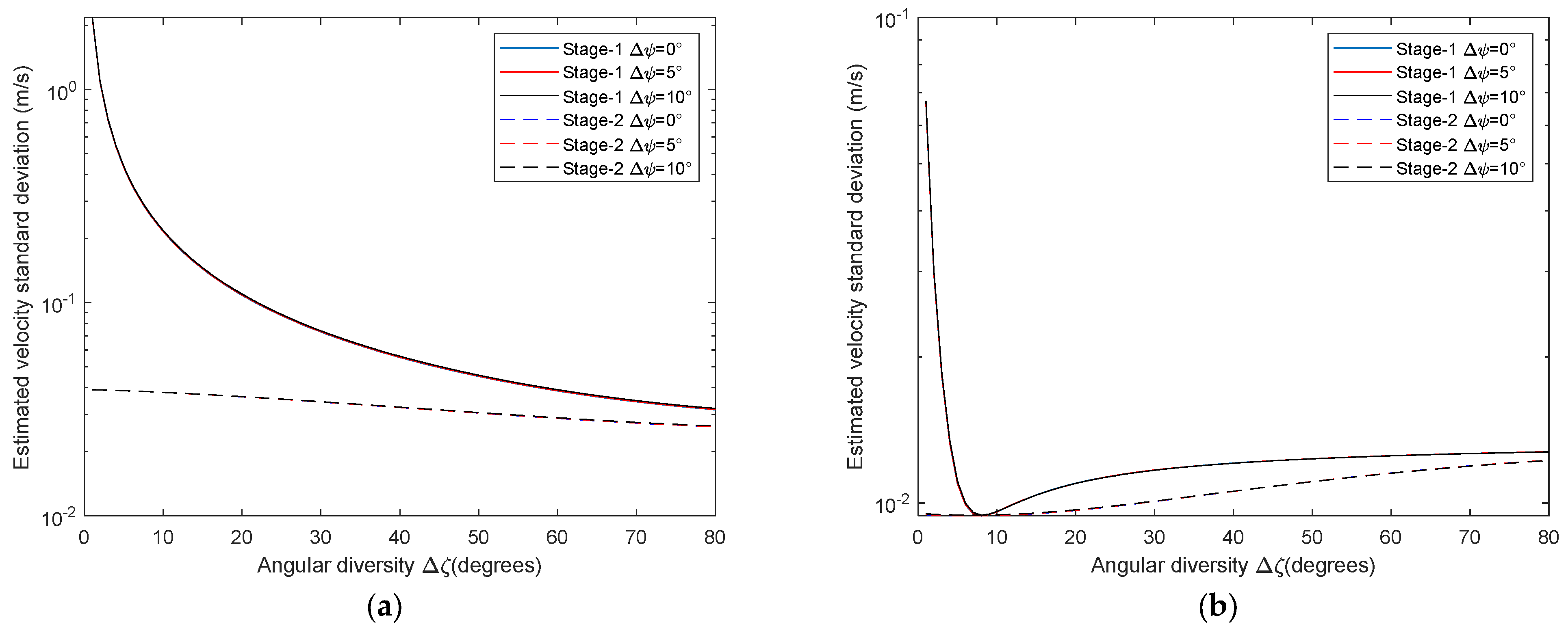
It could be noticed that complete information regarding translation is of paramount importance for maritime surveillance purposes and, in general, estimated kinematic parameters could be exploited also for classification/recognition. A few contributions can be found in the literature for rotational motion estimation (relevant for image scaling, if needed) [10,11] and for the estimation of the target trajectory (relevant also for motion compensation) [12,13,14,15]. This work fits into the latter category, addressing the estimation of the target translational motion capitalizing on the spatial diversity offered by multistatic ISAR configurations.
In this framework, in general, two different data fusion strategies can be followed, namely centralized or decentralized. In the former, the kinematic parameters are obtained directly from the fusion of the multi-sensor signals. This can be obtained in two different ways as follows:
(a)
By fusing at image level, i.e., single-sensor images in a single multi-sensor image. Along this line, a preliminary proof of concept for the case of two platforms with constrained geometry, considering only the slow-time domain, was shown in [14,15].
(b)
By fusing at the cost function level, i.e., a combination of multiple cost functions, each evaluated at the single-sensor level. Fusion at the cost function level was considered in [12,13] for multistatic autofocus.
However, decentralized data fusion architectures are often preferred in multistatic radar systems because of their larger robustness and scalability under different operative conditions. Noticeably, unlike centralized procedures, they do not require wideband communication links between the sensors [16]. Therefore, as an alternative to centralized approaches, we propose here a decentralized technique to accomplish the translational motion estimation task in multiplatform imaging systems; some preliminary results along this line were previously described in [17,18]. The proposed decentralized multistatic technique estimates the kinematic parameters via a two-step procedure: (1) first estimate the single-sensor signal parameters (Doppler centroid and Doppler rate); (2) then jointly exploit the estimated signal parameters to estimate the kinematic of the target. The second step is organized into two stages: the first stage is for velocity estimation, while the second one is for velocity estimation refinement (if a constant velocity model motion can be regarded as acceptable or, for acceleration estimation, if a constant velocity assumption does not apply). The selection between the two motion models is ruled by a decision criterion properly defined. It could be noticed that a decentralized approach could be suitable as a stand-alone technique (providing the estimates of the target motion parameters) or to initialize centralized techniques (providing the initial guess of the target motion parameters that can then be refined by centralized estimation approaches). The theoretical performance is analytically derived in terms of the covariance matrices of the estimates parameters (i.e., the single-sensor target signal parameters, Doppler frequency and Doppler rate, and the target kinematic parameters, velocity, and acceleration); theoretical results are completed and confirmed by using synthetic data. Performance is then assessed against a number of varying conditions and compared to the performance of alternative approaches from the literature. Particularly, the impact of the spatial diversity among the sensors on the achievable performance is investigated. Regarding the comparison, the performance of the proposed technique is also compared to that achievable by a centralized approach at the cost function level. This alternative approach has been selected as it can be suitable for both co-located and widely separated sensors, as the proposed decentralized technique, whereas the centralized technique at the image level is suitable for the co-located case only. Finally, to further prove the effectiveness and demonstrate the practical applicability of the proposed techniques, results obtained by applying them to live multistatic ISAR data are also shown.
The remainder of the paper is organized as follows: in Section 2, the multi-sensor system geometry and the echo model are introduced; in Section 3, the proposed multistatic estimation techniques are presented and their performance is theoretically analyzed in Section 4 and assessed in Section 5; Section 6 shows the results achieved against live multistatic data sets; and Section 7 concludes the paper. Analytical details are reported in the appendices.

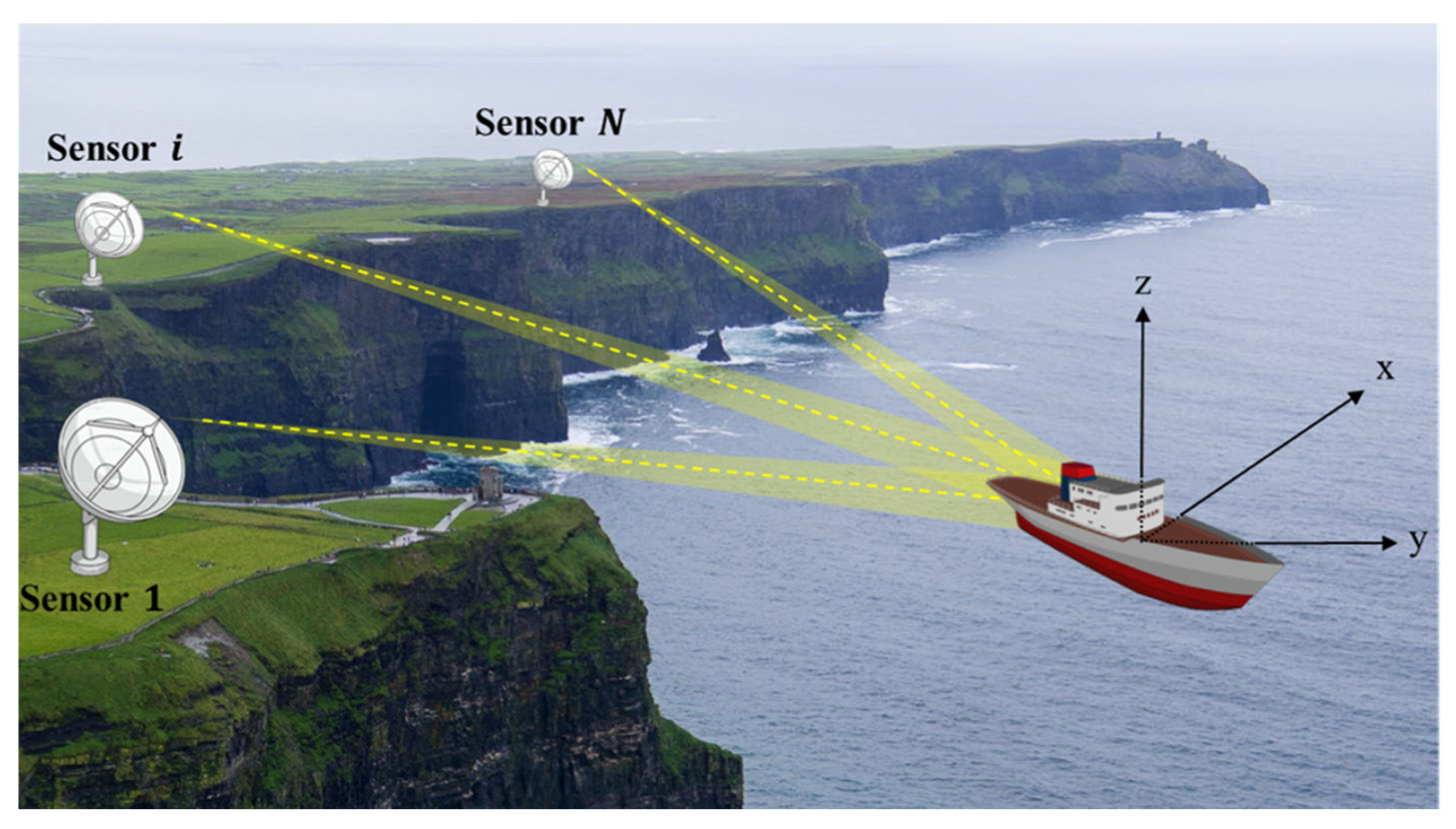
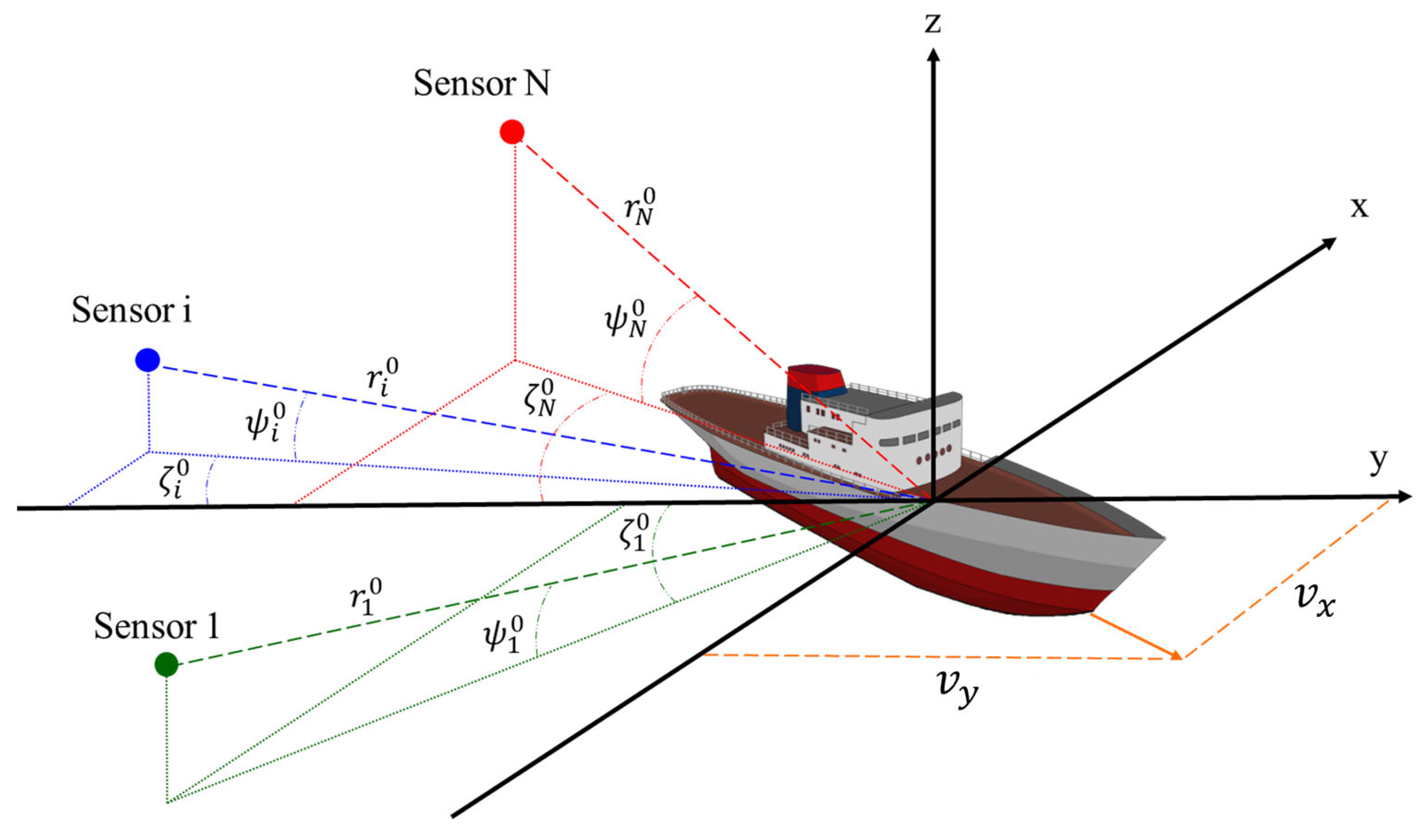
2. Geometry and Signal Model

In this work, we mainly refer to maritime scenarios. Figure 1 shows a pictorial view of the selected reference scenario comprising a coastal multistatic ISAR system and a vessel sailing in its field of view. However, it is worth underlining that the work could be easily generalized to cope with other scenarios and/or different targets.
Specifically, a formation of N sensors is considered; sensor 1 is a monostatic active radar system transmitting and receiving while the remaining N 1 are receiving only devices. In this case, N acquisitions are provided by the sensor network; one monostatic acquisition, from sensor 1, and N 1 bistatic acquisitions, each arising from the transmission from sensor 1 and reception from sensor i   ( i = 2 , , N ) . The ship is modeled as a rigid body; therefore, as usual in ISAR literature, its motion is decomposed as the translation of an arbitrary reference point and the rotation of the body around that point (hereafter named target fulcrum). Figure 2 shows the considered acquisition geometry in a fulcrum-centered reference system.
In such a system, r i ( t )   represents the position vector, changing with time, of sensor i , being ψ i ( t ) and ζ i ( t ) , respectively, which are the grazing angle and the angle between the projection on the X Y plane of the line-of-sight (LOS) and the y-axis (measured counter-clockwise from the y-axis). At image time (i.e., the synthetic aperture center here assumed as t = 0 without loss of generality), the position of sensor i is specified by:
r i ( 0 ) = [ x i 0 y i 0 z i 0 ] = r i 0 [ sin ζ i 0 cos ψ i 0 cos ζ i 0 cos ψ i 0 sin ψ i 0 ]
The target translation motion is taken into account by introducing the velocity vector v and the acceleration vector a . As we are dealing with ship targets, the vertical component of both velocity and acceleration is assumed negligible so that we can write v = [ v x   v y   0 ] T and a = [ a x   a y   0 ] T , however, the approach could be easily generalized to cope with situations where a vertical motion component also has to be included. As usually performed, the distance of the target fulcrum from sensor i as a function of the slow-time t can be approximated in second order as:
r i ( t ) r i 0 + r ˙ i 0 t + r ¨ i 0 t 2 2
where r ˙ i 0 and r ¨ i 0 are the distance first and second derivatives evaluated at t = 0 , and λ is the wavelength. It is easy to show that, for the assumed geometry and target motion, these derivatives can be written as [19]:
r ˙ i 0 = cos ψ i 0 ( v x sin ζ i 0 + v y cos ζ i 0 )
r ¨ i 0 = cos ψ i 0 ( a x sin ζ i 0 a y cos ζ i 0 ) + 1   r i 0 sin 2 ψ i 0   ( v x 2 + v y 2 ) + 1   r i 0 cos 2 ψ i 0   ( v x cos ζ i 0 + v y sin ζ i 0 ) 2
On this basis, the two-way Doppler centroid and Doppler rate at the i-th sensor are written as f i = ( r ˙ 1 0 λ + r ˙ i 0 λ ) and f ˙ i = ( r ¨ 1 0 λ + r ¨ i 0 λ ) , respectively.

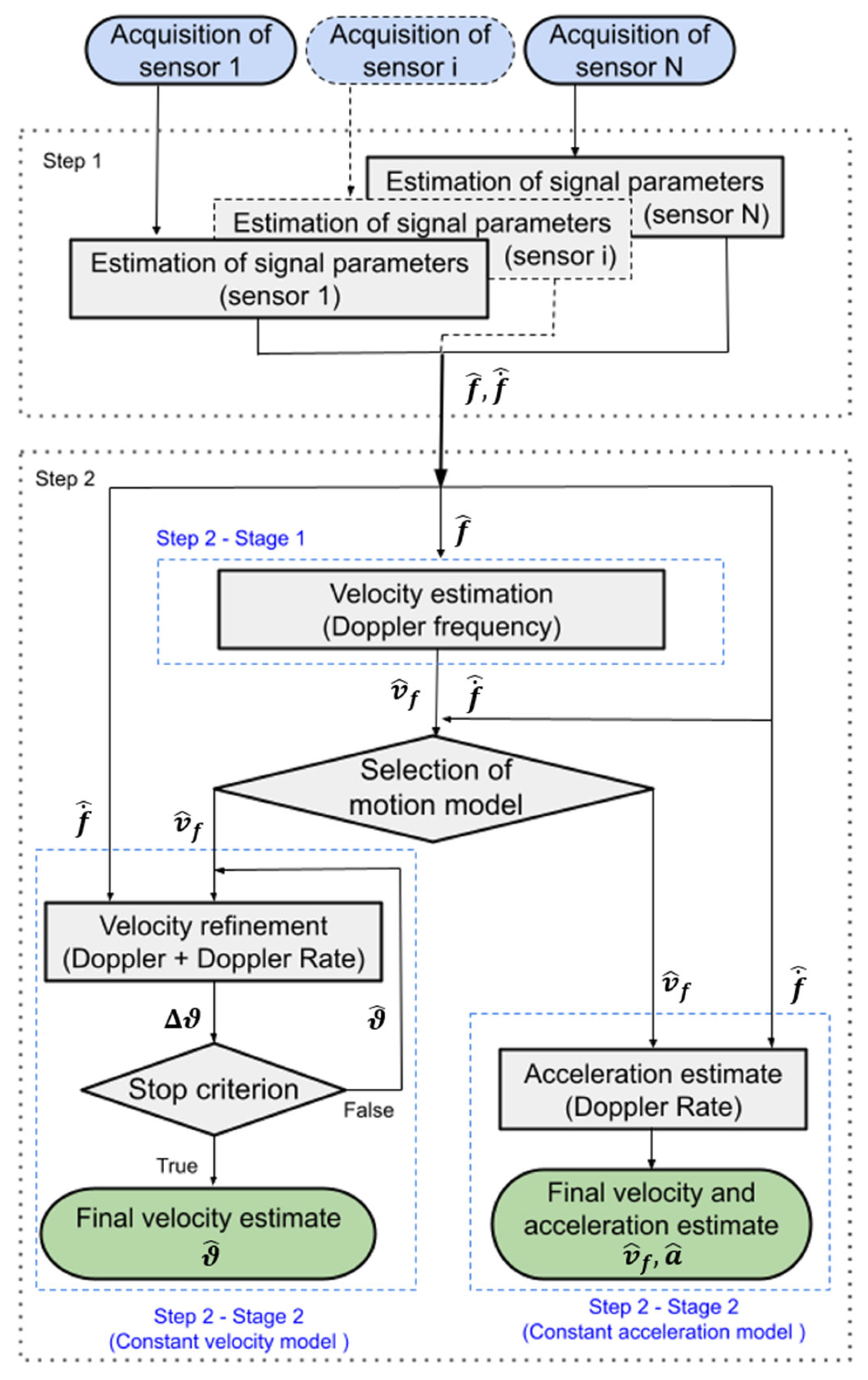
3. Multistatic Translational Motion Estimation Technique

Considering the availability of a multistatic ISAR system, in this work, we address the estimation of the target translation motion parameters by means of a two-step procedure:
  • Step 1: The first step is aimed at estimating the signal parameters (basically Doppler centroid and Doppler rate) at the single-sensor level;
  • Step 2: The second step is aimed at estimating the target motion parameters by inverting their analytical relationship with the target signal parameters. This step comprises two possibilities as the specific analytical relation depends on the assumed model for the target motion (the choice between the two is driven by a proper target motion model selection criterion).
The complete decentralized processing scheme is shown in Figure 3. Details concerning the two steps and the adopted selection criterion are provided in the following sub-sections.

3.1. Single-Sensor Signal Parameters Estimation Technique

From the geometry and signal model introduced in Section 2, it is apparent that, depending on the values of the integration time ( T ) of the vessel-specific motion, the transmitted signal bandwidth ( B ), and the relative position of the sensor with respect to the target, both the range and Doppler cell migration might be observed in the acquired single-sensor raw data; particularly, range migration is highly dependent from the Doppler centroid (range walk component), while Doppler migration is basically due to the Doppler rate. Therefore, these two single-sensor signal parameters, Doppler centroid and Doppler rate, are thus estimated as those values providing the single-sensor target image with the highest quality. In this work, as common in the ISAR literature, we resort to contrast maximization [20] but also other cost functions could be adopted (for example, entropy minimization [21]).
Since, for the application under consideration, the target size is limited to say about one hundred meters and we are not dealing with very high resolution, we consider here a processing technique that exactly compensates the migration through the range and Doppler cells for the ship fulcrum and then it images the target via Fourier transform (i.e., rectangular format). Specifically, starting from single-sensor data in the range-compressed, slow-time domain, the range migration correction is performed by compensating at slow time instant ( t ) for a fast-time delay given by v r t c , where v r  is the generic radial velocity, and c is the speed of light. By expressing the generic radial velocity in terms of the generic value for the Doppler centroid ( f ˜ ) ,  such a delay can be rewritten as f ˜ λ t c = f ˜ t f c , with f c being the carrier frequency. Therefore, the correction is performed in the fast-frequency and slow-time domain by multiplying the transformed data by:
Φ 1 ( f τ , t , f ˜   ) = e x p ( j 2 π f τ f ˜ f c t )
with f τ being the fast-frequency. The following step is a range inverse Fourier transform to map back the data in the range-compressed and slow-time domain, where they are multiplied with a reference chirp signal (i.e., data dechirping):
Φ 2 ( t , f ˙ ˜   ) = e x p ( j π f ˙ ˜ t 2 )
with f ˙ ˜ being the generic value for the Doppler rate. Finally, an azimuth Fourier transform is performed to obtain the data in the image domain. Let I i ( f ˜ , f ˙ ˜ ) be the intensity value of this i -th single-sensor complex image by defining the image contrast as:
I C i ( f ˜ , f ˙ ˜ ) = E { [ I i ( f ˜ , f ˙ ˜ ) E ( I i ( f ˜ , f ˙ ˜ ) ) ] 2 } E ( I i ( f ˜ , f ˙ ˜ ) )
where the operator E { · } represents the image spatial mean. The final Doppler and Doppler rate estimates at sensor i are obtained by maximizing the contrast.
( f ^ i , f ˙ ^ i ) = a r g m a x f ˜ , f ˙ ˜ { I C i ( f ˜ , f ˙ ˜ ) }

3.2. Kinematic Parameters Estimation Technique

The second step is organized into two stages: the first stage is for velocity estimation, while the second one is for velocity estimation refinement. If a constant velocity model motion can be regarded as acceptable, or for acceleration estimation, a constant velocity assumption does not apply. The decision between the two motion models is performed according to the criterion described in Section 3.3.

3.2.1. Kinematic Parameters Estimation Technique—Stage 1

Starting from the first stage, considering the formation of N sensors and using a matrix notation and results in Section 2, we can write:
f = G v
where f ^ is the N × 1 vector collecting the N estimated Doppler centroids, v = [ v x   v y ] T , and G is a N × 2 matrix taking into account the specific acquisition geometry:
G = 1 λ [ 2 cos ψ 1 0 sin ζ 1 0 2 cos ψ 1 0 cos ζ 1 0 cos ψ 1 0 sin ζ 1 0 + cos ψ 2 0 sin ζ 2 0 cos ψ 1 0 cos ζ 1 0 cos ψ 2 0 cos ζ 2 0 cos ψ 1 0 sin ζ 1 0 + cos ψ N 0 sin ζ N 0 cos ψ 1 0 cos ζ 1 0 cos ψ N 0 cos ζ N 0 ]
Exploiting the Doppler frequencies estimated in step 1, and assuming the knowledge of the acquisition geometry, the target velocity is obtained as the least square (LS) solution of the system in Equation (9), thus obtaining:
v ^ f = ( G T G ) 1 G T f ^ = G # f ^
where ( ) # denotes the pseudo-inverse operator.

3.2.2. Kinematic Parameters Estimation Technique—Stage 2

As stated above, in the second stage, if a constant velocity motion model can be regarded as acceptable, the velocity estimated at the previous step is refined by incorporating the Doppler rate information, otherwise, the velocity estimated at stage 1 is retained as the final estimate, and the Doppler rate information is exploited to estimate the acceleration.
Starting from the case of constant velocity, the exploitation of the Doppler rate measurements requires the solution of a system of N non-linear equations in two unknowns:
{ f ˙ ^ i = 2   r 1 0 λ sin 2 ψ 1 0   v x 2 + v y 2 + cos 2 ψ 1 0   v x cos ζ 1 0 + v y sin ζ 1 0 2 f ˙ ^ i = 1   r 1 0 λ sin 2 ψ 1 0   v x 2 + v y 2 + cos 2 ψ 1 0   v x cos ζ 1 0 + v y sin ζ 1 0 2 1   r i 0 λ sin 2 ψ i 0   v x 2 + v y 2 + cos 2 ψ i 0   v x cos ζ i 0 + v y sin ζ i 0 2 f ˙ ^ N = 1   r 1 0 λ sin 2 ψ 1 0   v x 2 + v y 2 + cos 2 ψ 1 0   v x cos ζ 1 0 + v y sin ζ 1 0 2 1   r N 0 λ sin 2 ψ N 0   v x 2 + v y 2 + cos 2 ψ N 0   v x cos ζ N 0 + v y sin ζ N 0 2
The system in Equation (12) can be linearized by using a first-order Taylor series approximation around a generic target tentative velocity, ϑ 0 = [ v x 0   v y 0 ] T :
f ˙ ^ f ˙ ( ϑ 0 ) = H · ( ϑ ϑ 0 )
where f ˙ ^   is the N × 1 vector collecting the N estimated Doppler rates, f ˙ ( ϑ 0 ) is the N × 1 vector collecting the N Doppler rates evaluated for the tentative velocity, ϑ = [ v x   v y ] T , and a matrix notation has been adopted based on the following definition:
H = [ f 1 ˙ v x f 1 ˙ v y f N ˙ v x f N ˙ v y     ] | ϑ = ϑ 0
The initial tentative value in this second stage could be chosen equal to the estimate provided by the first stage (i.e., initial ϑ 0 = v ^ f ), and the overall system to be solved is obtained by augmenting Equation (9) with the one in Equation (13), namely:
F ˙ ^ F ˙ ( ϑ 0 ) = [ 0 N × 1 f ˙ ^ f ˙ ( ϑ 0 ) ] = U · ( ϑ ϑ 0 )
where 0 N × 1  is a vector of N × 1 with all elements set to 0 and U is a 2 N × 2 block matrix equal to U = [ G T H T ] T . It is worth underlining that this joint use allows us to refine the estimate of the target velocity using both measured Doppler centroids and rates. The LS solution is thus given by:
ϑ ^ = ϑ 0 + U # ( F ˙ ( ϑ ) F ˙ ( ϑ 0 ) )
Then, through Equation (16), the target kinematic parameters are updated with respect to the tentative value ( ϑ 0 ) , and the procedure is reiterated until, at the generic iteration, the displacement δ v x 2 + δ v y 2 is within the requirements on the velocity accuracy or the maximum admitted number of iterations is reached. In the hypothesis of error-free measurements, this algorithm converges to the true target velocity components.
In case a constant velocity assumption does not apply, the second stage is instead devoted to the estimation of the acceleration, again by exploiting the Doppler rate information estimated in the first step. Using previous results and definitions and adopting, again, a matrix notation, we can write:
f ˙ ^ f ˙ ( v ^ f ) = G · a
where a = [ a x , a y ] T . The target acceleration is then estimated as:
a ^ = G # · ( f ˙ f ˙ v ( v ^ f ) )

3.3. Automatic Motion Model Selection Criterion

The automatic selection of the motion model is based on a comparison between the Doppler rate measurements and the Doppler rate values evaluated, assuming the velocity is equal to that estimated at stage 1 and null acceleration. Similar values imply the acceptable hypothesis of null acceleration so that the constant velocity motion model is selected. The other schema is selected in the opposite case. The similarity is assessed by means of the Mahalanobis distance by evaluating the distance between the error vector, collecting the differences of the Doppler rate values measured and theoretically evaluated, and a Normal distribution characterized by zero mean value and proper covariance matrix. Specifically, let Δ f   ˙  be the error Doppler rate vector defined as:
Δ f   ˙ = f ˙ ^ f ˙ ( v ^ f , a = 0 )
This error vector has zero mean. Additionally, since the Doppler rate measurements and v ^ f are independent variables, it is possible to write the covariance matrix of the Doppler rate error vector as follows:
Σ Δ f ˙ = Σ f ˙ ^ + Σ f ˙ ( v ^ f , a = 0 )  
where the two matrix components are specified in the following Equations (23) and (25) for Σ f ˙ ^ , and Equation (B8) for Σ f ˙ ( v ^ f , a = 0 )   . For decision-making purposes, the Mahalanobis distance is compared to a threshold K , i.e.,
Δ f ˙ T ( Σ Δ f ˙ ) 1 Δ f ˙   < >   K
and the constant velocity model is selected in case the distance is below the decision threshold. The K value is set in order to achieve a fixed probability value that, in case of actual constant velocity, the error Doppler rate vector lies within the corresponding ellipsoid. In Section 4.3, it is explained in detail how to set the value of K.

4. Theoretical Performance Analysis

In this section, the theoretical performance of the proposed technique is analytically derived. Furthermore, theoretical derivations are validated by comparison with simulated analysis. Performance achievable at the single-sensor level in the estimate of the signal parameters is considered first (Section 3.1). Following this, the performance in the estimate of the target kinematics parameters (Section 3.2) and the impact of the motion model selection (Section 3.3) are addressed.

4.1. Theoretical Performance Analysis—Step 1: Single-Sensor Signal Parameters

The performance in the estimate of the signal parameters is derived under the following assumptions: (i) statistical independence among the sensors; (ii) target described by a single dominant scatterer globally, taking into account the overall target Radar Cross Section (RCS); and (iii) negligible rotation motion. Particularly, assumption (ii) allows a closed-form performance derivation, and assumption (iii) allows to derive a benchmark for the achievable performance. These two limitations are then removed in section V where performance is assessed for an extended target and in the presence of 3D rotation motions.
Starting from the Doppler frequency measurements collected in the N × 1 vector f ^ , it can be demonstrated (see Appendix A) that the error of the estimates e f ^ i can be modeled as a zero-mean Gaussian random variable, i.e., e f ^ i ~ N ( 0 , σ f ^ i 2 ) , with a standard deviation equal to:
σ f ^ i = 72 ( 2 π ) 2 T 2 S N R i n t i ( B f c ) 2 = 6 ( 2 π ) 2 T 2 S N R i n t i · 12 ( B f c ) 2
where T is the aperture time, B is the bandwidth of the transmitted signal, f c is the carrier frequency, and S N R i n t i is the integrated signal-to-noise ratio (SNR) at sensor i (i.e., SNR evaluated in a single-sensor image domain). Interestingly, it can be noticed that Equation (22) can be decoupled as the product of two terms, the first one ( 6 ( 2 π ) 2 T 2 S N R i n t i ) representing the Cramer Rao bound for the performance achievable in the estimate of the frequency of complex signals having constant amplitude and polynomial phase, [22], and the second one ( 12 / ( B f c )   2 ) representing the impact on the performance of the estimation performed via optimization of the range migration correction.
Moving to the Doppler rate measurements collected in the N × 1 vector f ˙ ^ , the performance can be easily evaluated by recalling that the contrast optimization technique can achieve the Cramer Rao bound in selected conditions (i.e., when a single scatterer is exploited or when the multiple exploited scatterers share a similar SNR value) and in any case shows an efficiency very close to one, [23]. On this basis, the error in the estimate of the Doppler rate e f ˙ ^ i can be modeled as a zero-mean Gaussian random variable, i.e., e f ˙ ^ i ~ N ( 0 , σ f ˙ ^ i 2 ) , with a standard deviation equal to (Appendix A)
σ f ˙ ^ i = 1 π 90 S N R i n t i T 4
Furthermore, since the measurements at the different sensors are independent, the Doppler and Doppler rate covariance matrix are, respectively:
Σ f ^ = d i a g ( σ f ^ 1 2 , , σ f ^ N 2 )
Σ f ˙ ^ = d i a g ( σ f ˙ ^ 1 2 , , σ f ˙ ^ N 2 )
and due to the decoupling between Doppler frequency and Doppler rate [22], the covariance matrix of the measurements as a whole has a diagonal block structure and can be easily derived from the two above matrices.
To verify the theoretical derivations, a comparison against synthetic data is shown here. For this purpose, we define the following reference scenario used from now on (any modification will be duly mentioned): a formation of two sensors is considered with distances r 1 0 = r 2 0 = 10  km and aspect and grazing angles equal to ζ 1 0 = 2 ° , ζ 2 0 = 6 ° , ψ 1 0 = ψ 2 0 = 0 ° . In agreement with the study cases presented in [14,15], the active system is assumed to transmit a bandwidth of B = 100   MHz with a center frequency of fc = 10 GHz, a Pulse Repetition Frequency of P R F = 600   Hz , and 2048 pulses in the Coherent Processing Interval (CPI). The target moves with translational motion according to velocity v = [ 8   4   0 ] T   m / s , negligible acceleration, and a constant yaw rotation motion ω y = 1   d e g / s . The SNR is set to 33 dB (image domain).
Figure 4 shows the obtained results for 1000 independent trials. Particularly, the red and green ‘×’ markers represent the Doppler and Doppler rate measurements at sensor 1 and sensor 2, respectively. For comparison, the figure shows also the theoretical ellipse as achievable from Equations (22)–(25), and the ellipse derived from the measurements, both associated with a probability value equal to 0.99. A very good agreement is observed between theoretical and simulated results for both measured signal parameters, thus validating the analytical results.

4.2. Theoretical Performance Analysis for Step 2

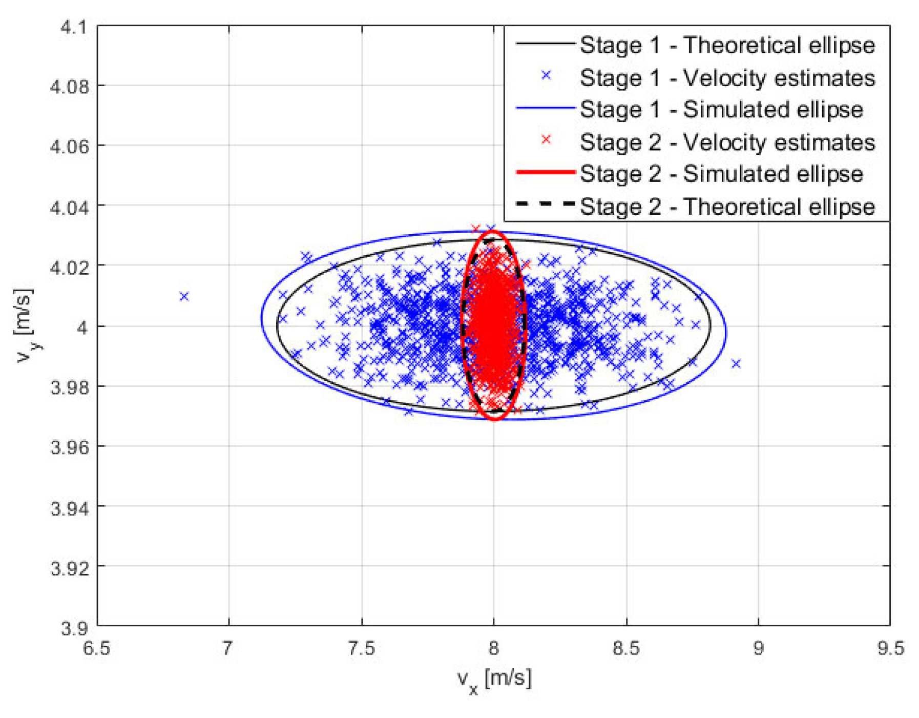
4.2.1. Step 2—Stage 1: Velocity Estimation

The covariance matrix of the velocity estimated at stage 1 can be derived by combining Equations (11) and (24):
Σ v ^ f = G # Σ f ^ G # T
Again, Figure 5 shows the estimated velocity components for 1000 independent trials and the same study case in Figure 4. Particularly, the blue markers represent the velocities as estimated at stage 1, the continuous black ellipse is the theoretical iso-level curve, and the blue one is the ellipse derived from the simulations, both referred to 0.99 probability. The statistics (the mean value and the standard deviation in x and y -directions, respectively) are shown in Table 1. Firstly, we observe, once again, a very good agreement between the theoretical predictions and the simulated results. Moreover, we notice how the accuracy in the estimation is higher for the y-component than for the x-component. This is a consequence of the exploitation of the Doppler frequency measurements that, in the considered case study (limited angular diversity between the two sensors), are highly dependent on v y , but scarcely sensible to v x .

4.2.2. Step 2—Stage 2: Velocity Refinement

The covariance matrix of the velocity estimated at stage 2 can be proven equal to (see Appendix B):
Σ ϑ ^ ( k ) = A ( k ) [ 0 2 N × 2 [ 0 N x N   Σ f ˙ ^ ] T ] A ( k ) T + B Σ v ^ f B T
where matrices A and B are defined as:
A ( k ) = i = 0 k 1 ( I U # | ϑ = ϑ 0 [ 0 N × 2 H | ϑ = ϑ 0 ] ) i U # | ϑ = ϑ 0
B = ( I U # | ϑ = ϑ 0 [ 0 N × 2 H | ϑ = ϑ 0 ] )
I is the identity matrix, k is the iteration at which the refinement is stopped, and the initial velocity ( ϑ 0 ) is the value provided by Equation (11). In order to analyze the impact of the refinement process on the estimation accuracy, Figure 6 shows the area of the theoretical 1σ ellipse associated with the covariance matrix in Equation (27) as a function of the iteration number for three geometry configurations: (i) narrow angular separation in blue ( ζ 1 0 = 2 ° and ζ 2 0 = 6 ° ), corresponding to the case previously discussed, (ii) medium angular separation in red ( ζ 1 0 = 6 ° and ζ 2 0 = 18 ° ), and (iii) wide angular separation in green ( ζ 1 0 = 12 ° and ζ 2 0 = 36 ° ).
From the figure, for all configurations, it can be observed a rapid improvement in the first iterations until a minimum value (identified in the figure with a triangle and named k m i n in the following) is reached. After this value, it is observed a slight increase. This characteristic is used to define a further stop criterion: based on Equation (27), the refinement process finishes after k m i n iterations.
The red crosses in Figure 5 represent the refined estimates corresponding to points coming from stage 1 (blue crosses). These results have been obtained by stopping the iterative procedure at k m i n . Table 2 compares the theoretical mean value and standard deviation of the stage 2 estimated velocity components to the values achieved by simulations. Again, the simulated results are well in line with the theoretical predictions. As expected, the exploitation of the Doppler rate measurements (highly sensitive to the velocity x-component) greatly increases the performance with respect to stage 1 for the x-component, whereas almost unvaried performance is obtained for the y-component. Overall, the joint exploitation of Doppler centroid and Doppler rate measurements allows the achievement of considerably high accuracy for both components.

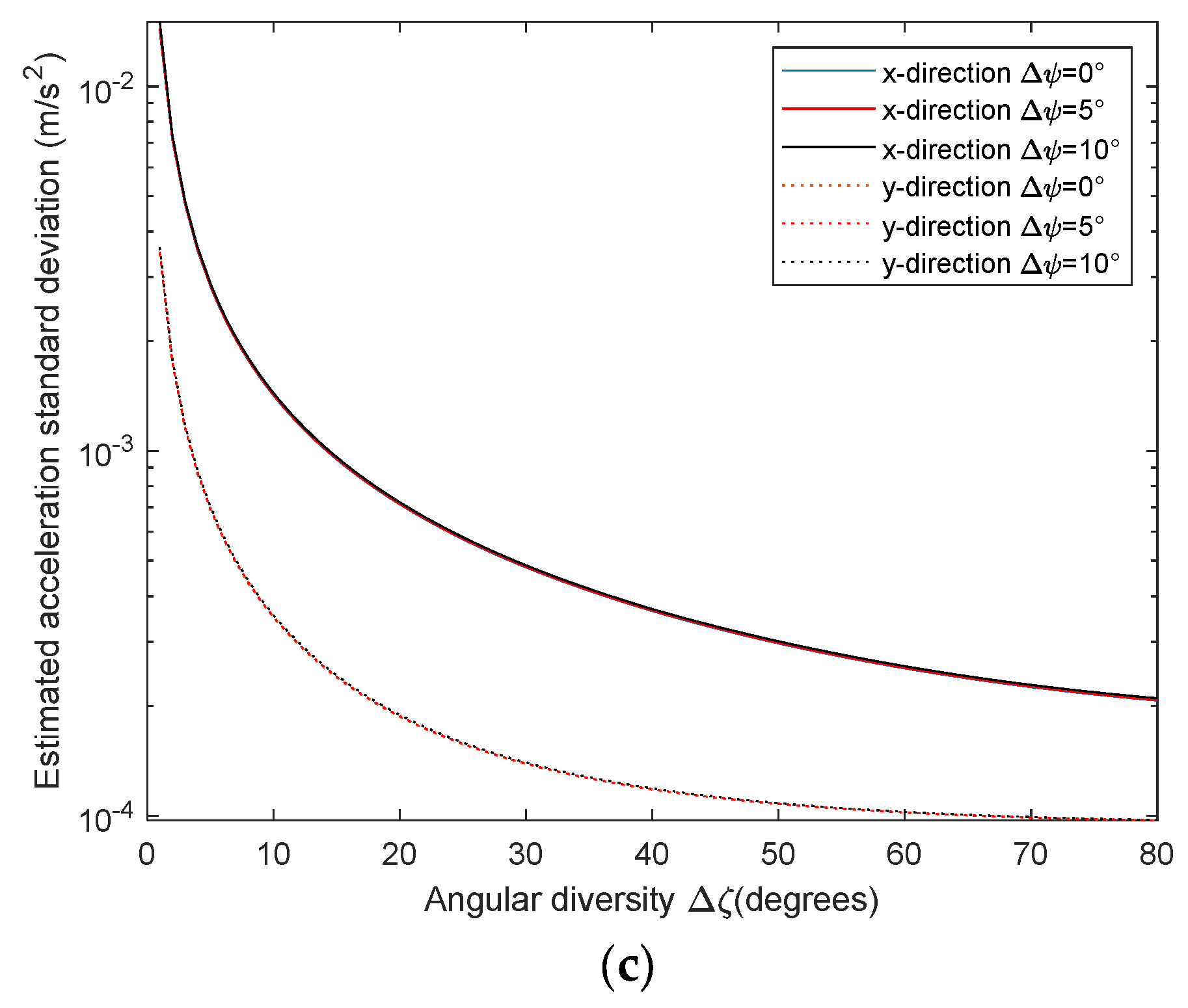
4.2.3. Step 2—Stage 2: Acceleration Estimation

The covariance matrix of the acceleration estimated at stage 2 can be proven equal to (see Appendix B):
Σ a = G # ( Σ f ˙ ^ + Σ f ˙ ( v ^ f , a = 0 )     ) G # T
with Σ f ˙ ( v ^ f , a = 0 )   = C   Σ v ^ f C T and C being the N × 2 matrix defined in the Appendix. In this case, to compare the theoretical predictions to the simulations, the previous reference scenario is maintained, but an acceleration a = [ 0.45   0.225   0 ] T   m / s 2 is also included. For this case, Figure 7 shows the estimated velocity (Figure 7a) and acceleration (Figure 7b) components with the superimposed corresponding ellipses, while Table 3 compares the theoretical and simulated mean values and standard deviations. The shown results once again confirm the validity and correctness of the theoretical derivations. Moreover, we can appreciate the high accuracy achievable by the proposed approach in the estimate of the acceleration components. This very good result is enabled by the exploitation of the Doppler rate measurements that are directly proportional to the acceleration showing high sensitivity with respect to its variations.

4.3. Automatic Motion Model Selection

As stated in Section 3.3, the motion model is selected by means of the decision rule in Equation (21). The constant velocity model is selected in case the distance is below the decision threshold, otherwise, an acceleration is estimated. The K value is set in order to achieve a fixed probability value that, in case of actual constant velocity, such a condition is correctly detected so that the velocity undergoes the refinement foreseen at stage 2. In particular, when the target is actually uniformly moving, the distance in Equation (21) is a random variable following a chi-square probability density function with N degrees of freedom. Therefore, the probability of correctly detecting this condition is provided by the chi-square cumulative distribution function:
P d ( K ,   N ) = γ ( N / 2 ,   K / 2 ) Γ ( N / 2 )
where γ ( ,   ) is the lower incomplete gamma function and Γ ( N / 2 ) is the gamma function, [24]. For the special case of two sensors ( N = 2 ) , the P d simplifies as follows:
P d ( K ,   N = 2 ) = 1 e K 2
The threshold value ( K ) has to be set in order to guarantee a reasonably high P d value, while at the same time keeping a good sensitivity to the presence of small acceleration values. In order to prove the effectiveness of the proposed approach, for the study case comprising two sensors, Figure 8 shows the probability of selecting an accelerated model for a target moving with a velocity equal to [8 4 0] m/s and variable acceleration ( a x , a y ) having set K so that P d = 0.99 . Figure 9 shows the probability of deciding on a uniform motion as a function of the acceleration in (a) x-direction and (b) y-direction for different P d ( K ) values. As evident from the results, the proposed approach is quite effective at discriminating between the two conditions; particularly in Figure 8 where the presence of an acceleration is correctly detected even in the presence of low values. Concerning the transition between the two decision regions, as expected, the higher the P d value, the larger the transition region is as it can be appreciated by inspecting Figure 9 which shows the cuts of Figure 8 along the a x and a y directions around a = 0 m/s2. Nevertheless, it is easy to observe that even in the presence of P d values close to 1 (i.e., 0.99), the decision test maintains a very good performance, assuring a high sensitivity.

5. Performance Assessment

5.1. Performance Assessment with Respect to SNR Conditions and Spatial Diversity

The performance for different SNR conditions is first investigated. Specifically, Figure 10a shows the standard deviation of stage 1 velocity in the x-direction (red curve) and the y-direction (blue curve) as a function of integrated (i.e., integrated over both fast and slow time and over the target scatterers) SNR values. When a constant velocity model is acceptable, the refined velocity of stage 2 exhibits the accuracy illustrated by the dashed curves in Figure 10a. Conversely, if a constant acceleration model is selected, the estimated acceleration demonstrates the performance indicated by the curves in Figure 10b.
As expected, higher integrated SNR values lead to improved estimation accuracy. Nevertheless, even for low/medium values of the SNR (we have to recall that the considered values refer to an integrated SNR and the ship has been already detected, so 20 dB is quite a low value for imaging purposes), good performance is achieved also by the stage 1 velocity estimation (that represents the initial value when the refinement in stage 2 is applied).
The performance of different sensor positions is now investigated. Particularly, for the study cases previously introduced, Figure 11a,b refers to the uniform motion case and shows the theoretical standard deviation of the estimated velocity as a function of the angular separation in aspect between the two sensors for different separations in grazing. Both stage 1 and stage 2 are shown. Figure 11c regards instead the performance in estimating the accelerations for the non-uniform case.
Starting from the case of uniform motion, from the curves shown in Figure 11a,b, it is possible to make the following observations: (i) in general the performances improve as the angular diversity in aspect increases and remain unchanged as the grazing diversity varies. This is a consequence of having assumed the target motion on the (x, y) plane (actually, the angular diversity in grazing would play a fundamental role in the estimation of the velocity along z); (ii) the improvement is marked in particular for stage 1, which, by exploiting only the Doppler information, fails to adequately estimate the cross velocity (x-direction) in the case of small diversity; and (iii) the estimate of the component in y reaches minimum standard deviation when both sensors observe the same radial component. In the case of accelerated motion, the performance improves as the diversity increases for both components. Consistently with the results shown above, the performance in estimating the component in y is in any case better than the estimation of the component in x as a consequence of the direct impact of component in y on the radial acceleration. In any case, even in the presence of limited angular diversity, good performance is obtained.

5.2. Performance Assessment with Respect to Extended Targets

The assumption of a target described by a single dominant scatterer globally, taking into account the overall target RCS, is now removed and the analysis is generalized considering the case of an extended ship target characterized by a number of dominant scatterers. The considered target model is shown in Figure 12. As in the previous analysis, the SNR is set to 33 dB (image domain) and the same motion conditions have been considered. Particularly, concerning SNR, to allow a comparison with the results for a point-like target, the contribution from each scatterer is scaled so that the integration among the different scatterers would result, again, in the same SNR value. This is obtained by considering the single scatterer reflectivity equal to a fraction (1/20) of the point-like reflectivity.
For the first tested case (uniform motion, velocity v = [ 8   4   0 ] T   m / s , and negligible acceleration), Figure 13 shows the obtained results for 1000 independent trials. As in the previous analyses, the blue crosses represent the estimated velocities at stage 1, while the red ones represent the estimates after the refinement at stage 2. For comparison, the same figure shows also, for both stages, the theoretical iso-level curves corresponding to 0.99 probability level and the corresponding ellipses containing 99% of the estimates. In addition, Table 4 compares the theoretical (point-like target) and simulated (extended target) mean value and standard deviation for both velocity components and both stages. From the shown results, it is easy to observe that, when moving from the ideal point-like to the extended target case (keeping fixed the overall SNR), the estimates are still unbiased but a slight degradation in terms of error standard deviation is observed. This is a consequence of more dispersed estimates of the Doppler frequency and Doppler rate at the single-sensor level, due to the interferences and also to the approximated procedure used in distributing the overall RCS among the scatterers. A similar degradation is observed on both the components.
For the second tested case (velocity v = [ 8   4   0 ] T   m / s and acceleration a = [ 0.45   0.225   0 ] T   m / s 2 ), Figure 14 shows the obtained results for 1000 independent trials. Particularly, Figure 14a represents the velocity components as estimated by the first stage, while Figure 14b shows the acceleration components as estimated using the first stage velocity and exploiting the Doppler rate information. Additionally, the theoretical ellipses are superimposed on the figures to compare the point-like and extended target performance. Table 5 shows the estimated statistics. From the shown results, also in this case, a small degradation is observed and similar considerations as those already performed for the uniform case can be applied.
Finally, the impact of the presence of a 3D rotation motion is analyzed. For this purpose, again, a simulated analysis has been carried out by also including sinusoidal pitch and roll motion with amplitudes of 0.25° and 1.25° and frequencies of 0.178 Hz and 0.091 Hz, respectively, [25]. The obtained results are reported in Table 4 for the case of uniform motion and in Table 5 for the case of accelerated motion. From the shown results, we can observe that the inclusion of a three-dimensional rotation introduces a slight polarization in the velocity and acceleration estimates, while the standard deviations remain almost unchanged. Anyway, despite the small degradation, in both cases we observe that very good performance is maintained.

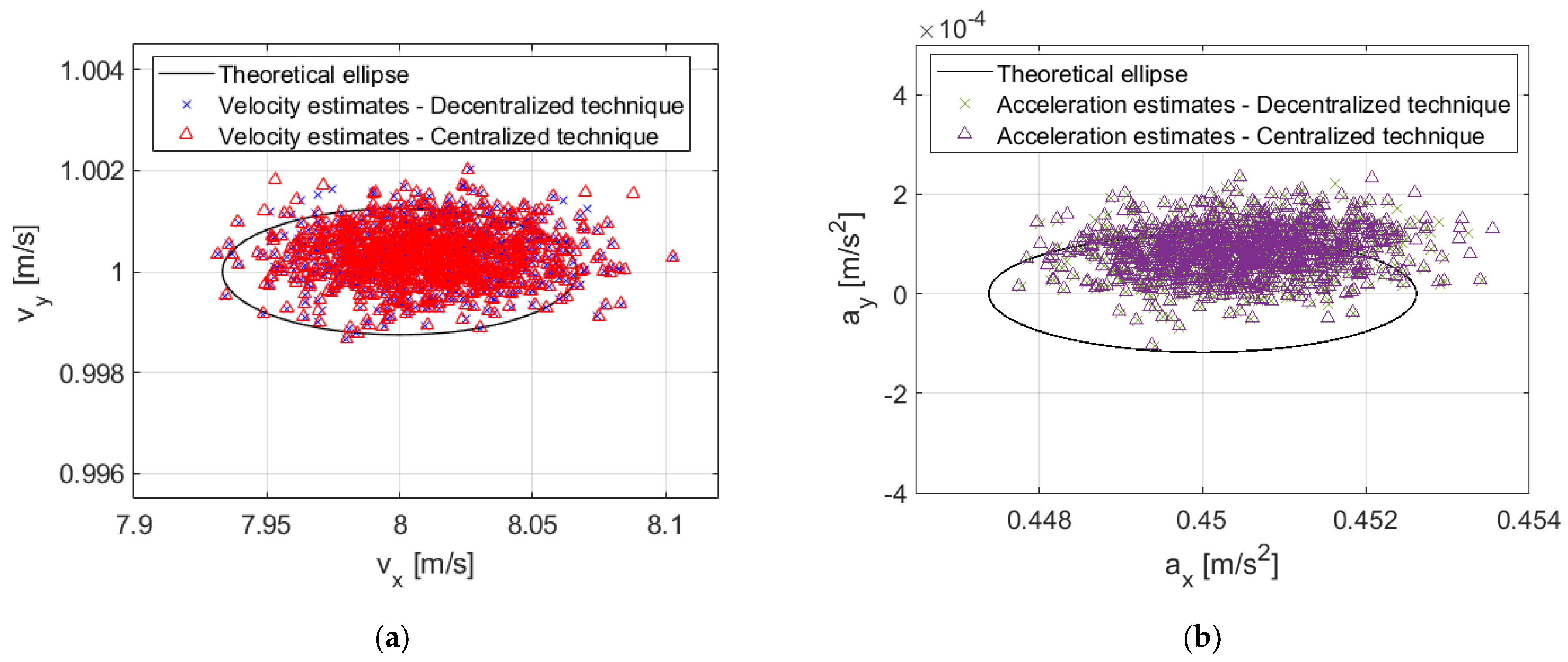
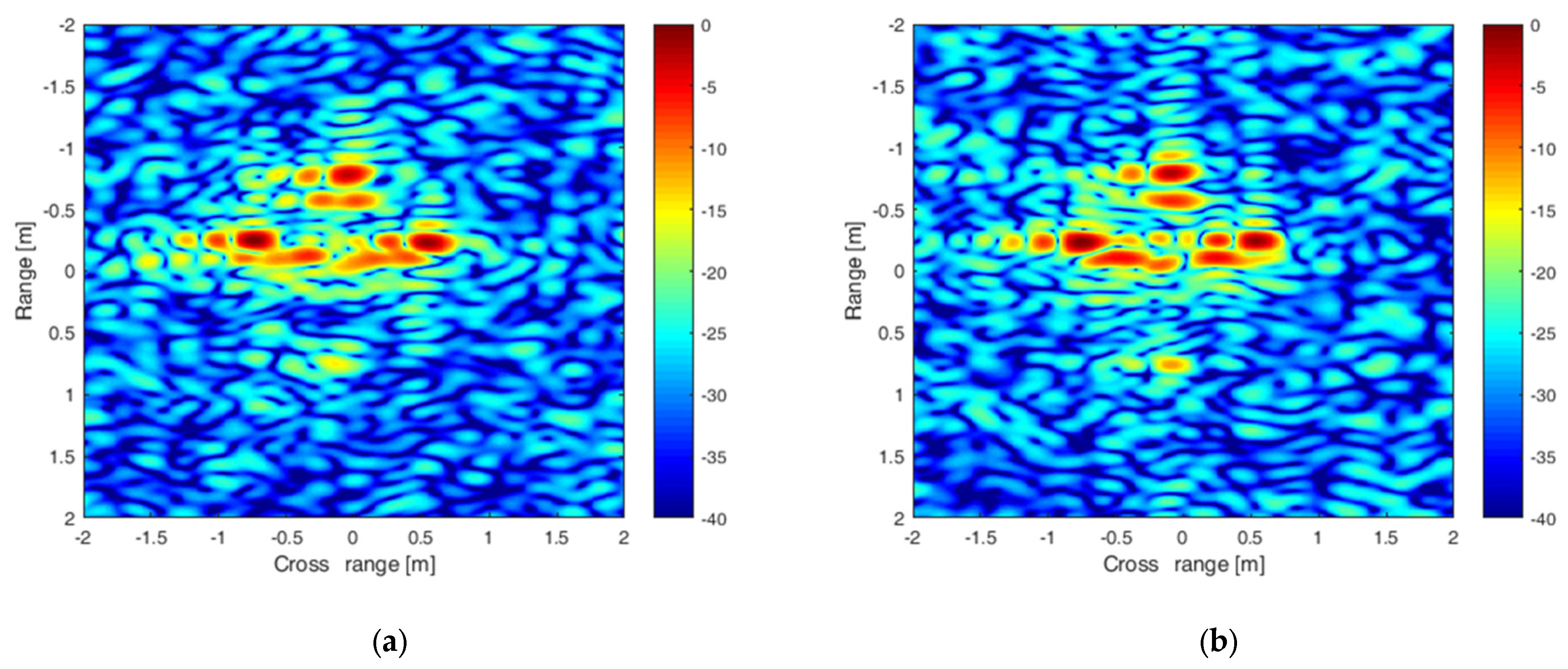
5.3. Performance Assessment with Respect to Centralized Approach

The performance of the proposed decentralized technique is now compared to that of a centralized approach at the cost function level that can be derived along the same line in [12,13]. In this case, the fusion of the multi-sensor signals is implemented at the cost-function level. Specifically, the single-sensor image contrast values are combined in a new multistatic cost function defined as the product of the individual cost functions, as illustrated in Figure 15. This centralized approach has been selected for performance comparison being, as the proposed one, suitable without restrictions with respect to the angular separation among the sensors.
The optimization problem to be solved for the multistatic case is therefore:
v ^ , a ^ = a r g m a x v , a { i = 1 N I C i ( v , a ) }
where I C i denotes the contrast of the image at the i -th sensor when motion is compensated according to the generic ( v , a ).
A drawback of this approach resides in the increased dimension of the space over which optimization has to be carried out. In our case, four parameters have to be estimated (two velocity and two acceleration components), thus resulting in a 4D optimization (2D when a constant velocity model is acceptable and 6D in a more general case, if also the vertical direction has to be included). This can represent a severe issue since the multistatic cost function can be expected to be multimodal, which generally represents a problem for the optimization algorithms to converge on the true solution.
To analyze the performance of the centralized and decentralized approaches, results against synthetic data are shown here. The same scenario explained in Section 4.1 is considered by testing two angular separations: (a) narrow angular separation (NAS), with aspect and grazing angles equal to ζ 1 0 = 2 ° , ζ 2 0 = 6 ° , ψ 1 0 = ψ 2 0 = 0 ° ; (b) wide angular separation (WAS), with aspect and grazing angles equal to ζ 1 0 = 10 ° , ζ 2 0 = 30 ° , ψ 1 0 = ψ 2 0 = 0 ° .
The extended target is assumed to be moving again with velocity being v = [ 8   4   0 ] T   m / s and acceleration being a = [ 0.45   0.225   0 ] T   m / s 2 . The multistatic cost function maximization in the centralized approach is implemented using the deterministic algorithm Nelder–Mead [26]. This algorithm requires an initial point as input and it is not guaranteed to converge to a global minimum/maximum. To deal with this problem, first, a range of possible velocity and acceleration values are defined. In our case, | v x | = | v y | < 15   [ m / s ] and | a x | = | a y | < 0.5   [ m / s 2 ] . Then, random velocity and acceleration values are generated within the allowed range and used as input parameters by the Nelder–Mead algorithm to maximize the multistatic cost function in Equation (33), obtaining the estimated target kinematic parameters as a result. The process is repeated for 200 randomly generated points. The final estimated values are selected as those that generate the highest value of the contrast product. Additionally, to also study the bound of performance achievable by means of the centralized approach, the case of an initial point equal to the true value of velocity and acceleration is also considered. Table 6 compares the mean value and the standard deviation of the estimated values for the decentralized technique, centralized technique with randomly selected initial point, and centralized with initial point coincident with the true value.
From the results for both velocity and acceleration, the following observations apply: (i) in all considered conditions, the decentralized technique achieves the same performance as the centralized one initialized with the true motion parameters; (ii) in WAS conditions, the decentralized approach outperforms the centralized technique with randomly selected initial values (this likely happens when the optimization over the 4D space, despite the high number of random initial points, does not converge to the good solution). These results confirm the effectiveness and robustness of the proposed approach which also has lower requirements from an implementation point of view (N 2D optimizations instead of a 4D optimization over an N factor function).

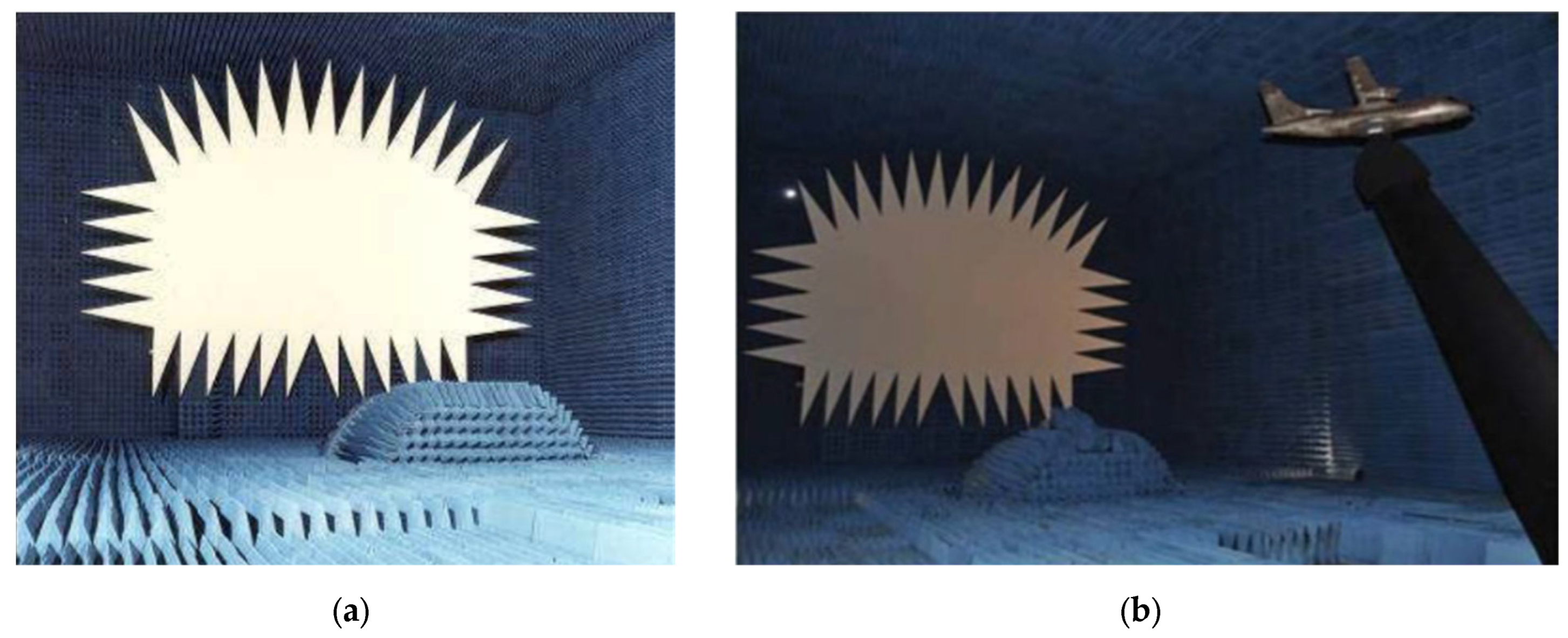
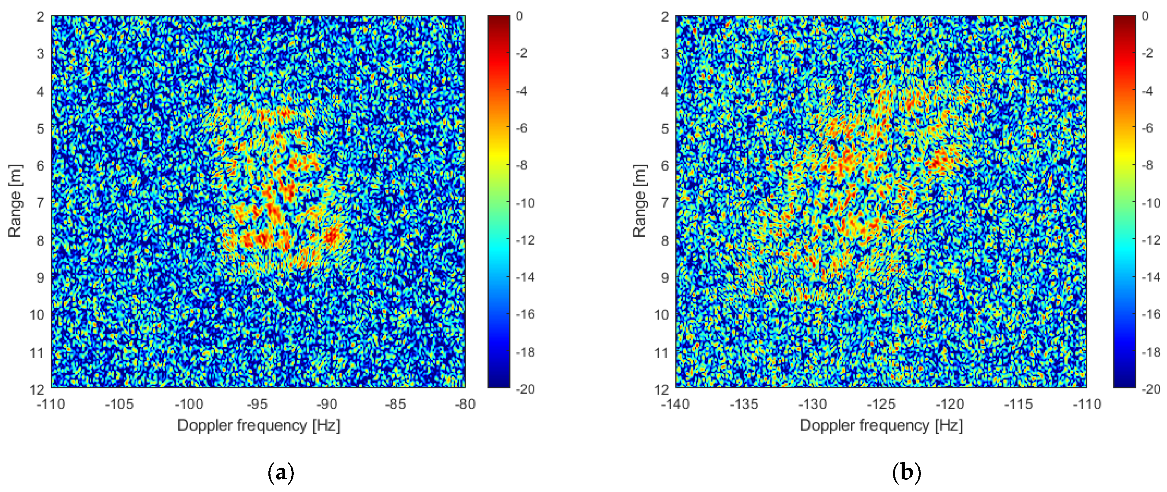
6. Experimental Results

In order to demonstrate the practical effectiveness of the proposed technique and validate the previous theoretical performance analysis, we apply both the decentralized and centralized techniques to multistatic ISAR data acquired in an experimental campaign carried out in an anechoic chamber at the SELEX Galileo facility in Caselle (Turin, Italy) [11].
The setup is based on the use of a single reflector Compact Range System which generates a planar wave front in the test zone. This includes the parabolic reflector, the feed system, and the positioner of the target under tests (TUT). The reflector (Figure 16a) is an offset parabolic reflector P/N 5755 made by Scientific Atlanta that, when illuminated by a spherical wave front transmitted by an antenna located into its focus (feed), generates a planar wave front on the TUT. Two HP 83622As are used for the transmitter and receiver signal sources, while the measurement instrumentation is based on an HP 8510C Network Analyzer. Chamber walls, ceilings, and floors are covered with absorber material (pyramid and wedge) to minimize unwanted reflections and diffractions. In this manner, a stray radiation level within the test zone below –35 dB is ensured.
The system transmits a stepped frequency waveform in the Ku-band ( 16.5   GHz ) with a fixed pulse-to-pulse frequency increment of Δ f = 3.75   MHz , resulting in an overall bandwidth of 3   GHz . The second receiver is located 60   cm from the transmitter, resulting in a bistatic channel having an aspect angle separation of Δ ζ = 4.3 ° with respect to the monostatic link. The turntable rotation yields an angular separation burst-to-burst of δ θ = 0.07 ° . The considered TUT is an ATR42 aircraft model (shown in Figure 16b) as representative of an extended target.
An overall illumination angle and bandwidth of Δ θ 5.18 ° and B = 1.5   GHz have been selected, respectively, resulting in a cross-range resolution ( ρ c r = λ 2 Δ θ = 10   cm ) and a range resolution ( ρ r = c / 2 B = 10   cm ). Referring to Figure 2, ζ 1 0 = 1 4 Δ ζ = 1.075 ° , ζ 2 0 = 3 4 Δ ζ = 3.225 ° and ψ 1 0 = ψ 2 0 = 0 ° . The experimental facility produces only a yaw rotational motion. Therefore, an emulated translational motion is superimposed on the acquired data according to velocity ( v = [ 8   1   0 ]   m / s ) and acceleration ( a = [ 0.45   0   0 ]   m / s 2 ). Furthermore, appropriately scaled noise is applied to achieve an integrated SNR of 33   d B . Figure 17 shows the resulting images. The defocusing effect, due to uncompensated translation motion, is quite visible.
These data are provided in input to the processing chain in Figure 3. Table 7 shows the mean and standard deviation of the estimates of the Doppler centroid and of the Doppler rate obtained at step 1 of the decentralized approach for 500 independent trails for both sensors and compares them to the corresponding theoretical performance. It is easy to observe a very good agreement between the theoretical predictions and the results obtained against the experimental data.
Figure 18 shows the estimated kinematic parameters. The blue (Figure 18a) and green (Figure 18b) crosses represent the velocity and acceleration components estimated by applying the decentralized approach, respectively. Additionally, the same parameters are estimated for the same 500 independent trails, but by applying the selected centralized approach with the optimization started from the actual velocity and acceleration values. The corresponding results are represented by red (Figure 18a) and violet (Figure 18b) triangles. Table 8 shows the mean and standard deviation as predicted by the theory and as obtained from the experimental data via the decentralized and centralized approach. We can observe that the achieved performance against the experimental data is well in line with the theoretical expectations. Additionally, in agreement with the results presented in Section 5.3, the proposed decentralized approach provides the same performance as that provided by the centralized fed with the actual kinematic parameters. Qualitatively similar results could be shown also for different (and in particular worst) SNR conditions (not reported here for the sake of compactness). These results further validate the effectiveness of the proposed technique and support its applicability in practical environments. Finally, Figure 19 shows an example of target images after motion compensation by using the estimated kinematic parameters, where the aircraft shape can be easily recognized in both the monostatic and bistatic ISAR images.

7. Conclusions

In this work, multi-sensor translational motion estimation techniques have been devised. A network formed by an active sensor and some passive devices has been considered and a decentralized two-step scheme proposed where the single-sensor, signal parameters are first estimated, and then this information is used in the second step to estimate the kinematic of the target. Particularly, Doppler measurements are used to make an initial velocity estimate, and when a constant velocity model is acceptable, Doppler rate information is exploited to provide a more accurate velocity estimate. If instead, via a proper decision rule, it is assessed that an acceleration has to be taken into account, such a decentralized approach estimates the acceleration by exploiting the initial velocity jointly with the Doppler rate information.
The performance of the proposed technique has been first analytically derived and then analyzed and assessed with respect to different conditions and parameters. Additionally, the proposed technique was compared with a centralized approach. The obtained results indicate that the decentralized technique provides the same performance as the centralized one operating in ideal conditions (i.e., the initial point for the optimization coinciding with the actual values of the parameters), and at the same time, lowering the complexity of the optimization problem. Finally, the techniques have been tested against experimental multi-sensor datasets and the results prove the suitability of the proposed approach for practical applications.

Author Contributions

Conceptualization, D.P. and F.S.; investigation, A.T.; software, A.T.; writing—original draft preparation, D.P.; writing—review and editing, F.S. All authors have read and agreed to the published version of the manuscript.

Funding

This research received no external funding.

Data Availability Statement

Not Applicable.

Conflicts of Interest

The authors declare no conflict of interest.

Appendix A. Analytical Derivation of Single-Sensor Target Signal Parameters Accuracy

Considering that the Doppler centroid and Doppler rate are decoupled parameters, we can separately derive the performance (performance calculation in Doppler assuming perfectly compensated Doppler rate and vice versa). In addition, for a single point-like target, it can be demonstrated that maximizing the intensity contrast is equivalent to maximizing its peak intensity [27]. On this basis, for the estimation of the Doppler centroid, it is possible to assume the signal in the slow-time range-frequency domain as:
y ( f ˜ 0 , f r i , t j ) = A e j 2 π f r i f ˜ 0 f c t j + n ( f r i , t j )
where i = 1 , , M and j = 1 , , N and n ( f r i , t j ) represents the background contribution modeled as white normal with zero mean value and variance σ n 2 . The estimated value is thus obtained as:
f ^ = max f ˜ | i j y ( f ˜ 0 , f r i , t j ) e j 2 π f r i f ˜ f c t j | 2
which can be rewritten as:
f ^ = max   f   ˜ i j h k y ( f ˜ 0 , f r i , t j ) y * ( f ˜ 0 , f r h , t k ) e j 2 π f r i f ˜ f c t j e j 2 π f r h f ˜ f c t k
The estimated value can be found by evaluating the first derivative and setting it equal to zero
f ˜ = max   f   ˜ i j h k y ( f ˜ 0 , f r i , t j ) y * ( f ˜ 0 , f r h , t k ) e j 2 π f r i f ˜ f c t j e j 2 π f r h f ˜ f c t k ( j 2 π f r i f c t j j 2 π f r h f c t k ) = 0
Assuming f ˜ f ˜ 0 + δ f ˜ (small errors) at the first order
e j 2 π f ˜ f c ( f r i t j f r h t k )   e j 2 π f ˜ 0 f c ( f r i t j f r h t k )   [ 1 + j 2 π δ f ˜ f c ( f r i t j f r h t k ) ]
Replacing Equations (A1) and (A5) in Equation (A4) and neglecting the second order term, we obtain:
i j h k [ A e j 2 π f r h f ˜ 0 f c t k n ( f r h , t k ) + A * e j 2 π f r i f ˜ 0 f c t j n ( f r i , t j ) ] j 2 π f c ( f r i t j f r h t k ) = i j h k | A | 2 δ f ˜ ( j 2 π f c ) 2 ( f r i t j f r h t k ) 2
Taking the expected value of both sides yields, < δ f ˜ > = 0, namely unbiased estimate. By considering the square of the term at the left side and evaluating its expected value, we have:
2 | A | 2 σ n 2 ( 2 π f c ) 2 M 3 N 3 B 2 12 T 2 12
while the term on the right side can be expressed as:
| A | 2 δ f ˜   2 ( 2 π f c ) 2 M 2 N 2 B 2 12 T 2 12
combining these yields the following result:
< ( δ f ˜ ) 2 > = 2 | A | 2 σ n 2 ( 2 π f c ) 2 M 3 N 3 B 2 12 T 2 12 [ | A | 2 2 ( 2 π f c ) 2 M 2 N 2 B 2 12 T 2 12 ] 2
from which Equation (22) is derived.
For the estimation of f ˙ , it is possible to consider the signal in the slow time domain as:
y ( f ˙ 0 , t j ) = A e j π f ˙ 0 t j 2 + n ( t j )
The estimated Doppler rate is thus obtained as:
f ˙ ^ = max f ˙ ˜ | j y ( f ˙ 0 , t j ) e j π f ˙ ˜ t j 2 | 2
Using the results of [27], it is possible to demonstrate that:
< δ f ˙ > = 0
< δ f ˙ 2 > = 1 π 2 90 S N R i n t T 4

Appendix B. Analytical Derivation of Stage 2 Estimated Velocity and Acceleration Covariance Matrices

Starting from the estimated velocity covariance matrix, from Equations (13)–(16), the relation between the errors at two successive iterations of the refinement can be written as follows:
Δ v i = U ϑ = v # [ 0 N × 1 f ˙ f ˙ ( v ) ] + ( I U ϑ = v # [ 0 N × 2 H ϑ = v ] ) Δ v i 1
Using the equation above, at first order, the error at the k -th iteration can be written in terms of the error at stage 1 (i.e., Δ v 0 = v ^ f v )
Δ v k = i = 0 k ( I U ϑ = v # [ 0 N × 2 H ϑ = v ] ) i U ϑ = v # [ 0 N × 1 f ˙ ^ f ˙ ( v ) ] + ( I U ϑ = v # [ 0 N × 2 H ϑ = v ] ) k Δ v 0 = A k [ 0 N × 1 f ˙ ^ f ˙ ( v ) ] + B k Δ v 0
A k and B k are defined as follows:
A k = i = 0 k ( I U ϑ = v # [ 0 N × 2 H ϑ = v ] ) i U ϑ = v #
B k = ( I U ϑ = v # [ 0 N × 2 H ϑ = v ] ) k
I is the 2 × 2 identity matrix, k is the iteration at which the refinement is stopped, and the initial velocity ( ϑ 0 ) is the value provided by Equation (11). Taking <   Δ v k Δ v k T > and considering the independence of the error at the first stage from the error in the estimate of the Doppler rates, Equation (27) is obtained.
To evaluate the covariance matrix of the estimated acceleration, we observe that the term f ˙ v ( v ^ f ) in Equation (18) has a quadratic dependence on the velocity and, therefore, can be written as:
f ˙ v i ( v ^ f ) = C 1 i v x 2 + C 2 i v y 2 + C 3 i v x v y
where C parameters depend only on the acquisition geometry. Linearizing the above equation around the real target velocity, it is possible to write the following approximation:
f ˙ v i ( v ^ f )   f ˙ i ( v 0 ) + ( 2 C 1 i v x 0 + C 3 i v y 0 )   δ v x + ( 2 C 2 i v y 0 + C 3 i v x 0 )   δ v y
Using a matrix notation, we can write:
[ f ˙ v 1 ( v ^ f ) f ˙ 1 ( v 0 ) f ˙ v N ( v ^ f ) f ˙ N ( v 0 ) ] = [ 2 C 1 1 v x 0 + C 3 1 v y 0 2 C 2 1 v y 0 + C 3 1 v x 0 2 C 1 N v x 0 + C 3 N v y 0 2 C 2 N v y 0 + C 3 N v x 0 ] [ δ v x δ v y ] = C [ δ v x δ v y ]
From Equations (18), (25), and (B7), and after simple manipulations, we obtain:
Σ a = G # ( Σ f ˙ ^ + C Σ v ^ f   C T ) G # T = G # ( Σ f ˙ ^ + Σ f ˙ ( v ^ f , a = 0 )     ) G # T

References

  1. Walker, J.L. Range-Doppler imaging of rotating objects. IEEE Trans. Aerosp. Electron. Syst. 1980, 16, 23–52. [Google Scholar] [CrossRef]
  2. Wehner, D.R. High-Resolution Radar, 2nd ed.; Artech House: Boston, MA, USA, 1992. [Google Scholar]
  3. Xu, X.; Narayanan, R.M. Three-dimensional interferometric ISAR imaging for target scattering diagnosis and modeling. IEEE Trans. Image Process. 2001, 10, 1094–1102. [Google Scholar] [PubMed]
  4. Rong, J.; Wang, Y.; Han, T. Interferometric ISAR Imaging of Maneuvering Targets With Arbitrary Three-Antenna Configuration. IEEE Trans. Geosci. Remote Sens. 2020, 58, 1102–1119. [Google Scholar] [CrossRef]
  5. Vehmas, R.; Neuberger, N. Inverse Synthetic Aperture Radar Imaging: A Historical Perspective and State-of-the-Art Survey. IEEE Access 2021, 9, 113917–113943. [Google Scholar] [CrossRef]
  6. Pastina, D.; Bucciarelli, M.; Lombardo, P. Multistatic and MIMO Distributed ISAR for Enhanced Cross-Range Resolution of Rotating Targets. IEEE Trans. Geosci. Remote Sens. 2010, 48, 3300–3317. [Google Scholar] [CrossRef]
  7. Zhu, Y.; Su, Y.; Yu, W. An ISAR Imaging Method Based on MIMO Technique. IEEE Trans. Geosci. Remote Sens. 2010, 48, 3290–3299. [Google Scholar]
  8. Pastina, D.; Santi, F.; Bucciarelli, M. MIMO Distributed Imaging of Rotating Targets for Improved 2-D Resolution. IEEE Geosci. Remote Sens. Lett. 2015, 12, 190–194. [Google Scholar] [CrossRef]
  9. Brisken, S.; Matthes, D.; Mathy, T.; Worms, J.G. Spatially diverse ISAR imaging for classification performance enhancement. Int. J. Electron. Telecom. 2011, 57, 15–21. [Google Scholar] [CrossRef]
  10. Santi, F.; Bucciarelli, M.; Pastina, D. Multi-sensor ISAR technique for feature-based motion estimation of ship targets. In Proceedings of the 2014 International Radar Conference, Lille, France, 13–17 October 2014; pp. 1–5. [Google Scholar]
  11. Santi, F.; Pastina, D.; Bucciarelli, M. Estimation of Ship Dynamics with a Multiplatform Radar Imaging System. IEEE Trans. Aerosp. Electron. Syst. 2017, 53, 2769–2788. [Google Scholar] [CrossRef]
  12. Brisken, S.; Martorella, M.; Mathy, T.; Wasserzier, C.; Worms, J.G.; Ender, J.H.G. Motion estimation and imaging with a multistatic ISAR system. IEEE Trans. Aerosp. Electron. Syst. 2014, 50, 1701–1714. [Google Scholar] [CrossRef]
  13. Brisken, S.; Martorella, M. Multistatic ISAR autofocus with an image entropy-based technique. IEEE Aerosp. Electron. Syst. Mag. 2014, 29, 30–36. [Google Scholar] [CrossRef]
  14. Bucciarelli, M.; Pastina, D.; Errasti-Alcala, B.; Braca, P. Multi-sensor ISAR technique for translational motion estimation. In Proceedings of the OCEANS 2015—Genova, Genova, Italy, 18–21 May 2015; pp. 1–5. [Google Scholar]
  15. Bucciarelli, M.; Pastina, D.; Errasti-Alcala, B.; Braca, P. Translational velocity estimation by means of bistatic ISAR techniques. In Proceedings of the 2015 IEEE International Geoscience and Remote Sensing Symposium (IGARSS), Milan, Italy, 26–31 July 2015; pp. 1921–1924. [Google Scholar]
  16. Goodman, N.A.; Bruyere, D. Optimum and decentralized detection for multistatic airborne radar. IEEE Trans. Aerosp. Electron. Syst. 2007, 43, 806–813. [Google Scholar] [CrossRef]
  17. Testa, A.; Santi, F.; Pastina, D. Translational motion estimation with multistatic ISAR systems. In Proceedings of the 2021 21st International Radar Symposium (IRS), Berlin, Germany, 21–22 June 2021; pp. 1–8. [Google Scholar]
  18. Testa, A.; Pastina, D.; Santi, F. Comparing decentralized and centralized approaches for translational motion estimation with multistatic ISAR systems. In Proceedings of the 2022 23rd International Radar Symposium (IRS), Gdansk, Poland, 12–14 September 2022; pp. 447–452. [Google Scholar]
  19. Raney, R.K. Synthetic aperture imaging radar and moving target. IEEE Trans. Aerosp. Electron. Syst. 1971, 7, 499–505. [Google Scholar] [CrossRef]
  20. Martorella, M.; Berizzi, F.; Haywood, B. Contrast maximisation based technique for 2-D ISAR autofocusing. IEE Proc. Radar Sonar Navig. 2005, 152, 253–262. [Google Scholar] [CrossRef]
  21. Xi, L.; Guosui, L.; Ni, J. Autofocusing of ISAR images based on entropy minimization. IEEE Trans. Aerosp. Electron. Syst. 1999, 35, 1240–1252. [Google Scholar] [CrossRef]
  22. Peleg, S.; Porat, B. The Cramer-Rao lower bound for signals with constant amplitude and polynomial phase. IEEE Trans. Signal Process. 1991, 39, 749–752. [Google Scholar] [CrossRef]
  23. Pastina, D. Rotation motion estimation for high resolution ISAR and hybrid SAR/ISAR target imaging. In Proceedings of the 2008 IEEE Radar Conference, Rome, Italy, 26–30 May 2008; pp. 1–6. [Google Scholar]
  24. Abramovitz, M.; Stegun, I.A. Handbook of Mathematical Functions, 3rd ed.; Dover Publications: New York, NY, USA, 1964. [Google Scholar]
  25. Bucciarelli, M.; Pastina, D. Multi-grazing ISAR for side-view imaging with improved cross-range resolution. In Proceedings of the 2011 IEEE RadarCon (RADAR), Kansas City, MO, USA, 23–27 May 2011; pp. 939–944. [Google Scholar]
  26. Lagarias, J.C.; Reeds, J.A.; Wright, M.H.; Wright, P.E. Convergence Properties of the Nelder-Mead Simplex Method in Low Dimensions. SIAM J. Opt. 1998, 9, 112–147. [Google Scholar] [CrossRef]
  27. Green, J.F.; Oliver, C.J. The limits on autofocus accuracy in SAR. Int. J. Remote Sens. 1992, 13, 2623–2641. [Google Scholar] [CrossRef]
Figure 1. Coastal multistatic ISAR system.
Remotesensing 15 04372 g001
Figure 2. Multistatic acquisition geometry.
Remotesensing 15 04372 g002
Figure 3. Decentralized processing scheme.
Remotesensing 15 04372 g003
Figure 4. Step 1 performance analysis: (a) Sensor 1 and (b) Sensor 2.
Remotesensing 15 04372 g004
Figure 5. Estimated velocity–Theoretical and sampled ellipses.
Remotesensing 15 04372 g005
Figure 6. Area of the theoretical 1σ ellipse versus the number of iterations.
Remotesensing 15 04372 g006
Figure 7. Estimated (a) velocity and (b) acceleration with theoretical and sampled ellipses.
Remotesensing 15 04372 g007
Figure 8. Motion model selection performance for variable acceleration and P d = 0.99 .
Remotesensing 15 04372 g008
Figure 9. Probability to detect uniform motion as a function of the acceleration in (a) x-direction and (b) y-direction for different P d (K) values.
Remotesensing 15 04372 g009
Figure 10. Performance assessment with respect to SNR: (a) estimated velocity, both stage 1 and stage 2, and (b) estimated acceleration.
Remotesensing 15 04372 g010
Figure 11. Performance assessment with respect to angular diversity: (a) estimated velocity x-direction, (b) estimated velocity y-direction, and (c) estimated acceleration both x- and y-direction.
Remotesensing 15 04372 g011aRemotesensing 15 04372 g011b
Figure 12. Multi-scatterer ship model. Top and side views.
Remotesensing 15 04372 g012
Figure 13. Initial and final estimated velocity–Extended target.
Remotesensing 15 04372 g013
Figure 14. Extended target–Constant acceleration model: (a) velocity and (b) acceleration.
Remotesensing 15 04372 g014
Figure 15. Centralized processing approach.
Remotesensing 15 04372 g015
Figure 16. Experimental setup: (a) compact range reflector and (b) target under test. ATR42 aircraft model (1:20 scale).
Remotesensing 15 04372 g016
Figure 17. Defocused and noisy target image at monostatic (a) and bistatic (b) sensor.
Remotesensing 15 04372 g017
Figure 18. Experimental extended target–Estimated (a) velocity and (b) acceleration.
Remotesensing 15 04372 g018
Figure 19. Target images after motion compensation (a) monostatic sensor and (b) bistatic sensor.
Remotesensing 15 04372 g019
Table 1. Mean and standard deviation—Stage 1 velocity.
StatisticsTarget Kinematic
Parameters
Theoretical ValuesDecentralized
Approach Estimates
mean v x   [ m / s ] 8.0008.001
v y   [ m / s ] 4.0003.999
std v x   [ m / s ] 0.2690.289
v y   [ m / s ] 0.0090.010
Table 2. Mean and standard deviation of the estimated stage 2 velocities–Point-like target.
StatisticsTarget Kinematic
Parameters
Theoretical ValuesDecentralized
Approach Estimates
mean v x   [ m / s ] 8.0008.001
v y   [ m / s ] 4.0003.999
std v x   [ m / s ] 0.0380.040
v y   [ m / s ] 0.0090.010
Table 3. Mean and standard deviation of the estimated velocity and acceleration–Point-like target.
StatisticsTarget Kinematic
Parameters
Theoretical ValuesDecentralized
Approach Estimates
mean v x   [ m / s ] 8.0007.986
v y   [ m / s ] 4.0004.001
a x   [ m / s 2 ] 0.4500.450
a y   [ m / s 2 ] 0.2250.225
std v x   [ m / s ] 0.2690.289
v y   [ m / s ] 0.0090.010
a x   [ m / s 2 ] 0.0020.002
a y   [ m / s 2 ] 0.0000.000
Table 4. Mean and standard deviation of the estimated velocity–Extended target and uniform motion.
StatisticsTarget Kinematic
Parameters
Stage 1 VelocityStage 2 Velocity
Theoretical Values
(Point like
Target)
Simulated
(Extended Target with Constant Yaw Rotation)
Simulated
(Extended
Target with 3D Rotation)
Theoretical Values
(Point like Target)
Simulated
(Extended Target with Constant Yaw Rotation)
Simulated
(Extended
Target with 3D
Rotation)
mean v x   [ m / s ] 8.0008.0097.6898.0008.0018.047
v y   [ m / s ] 4.0003.9994.0334.0003.9994.033
std v x   [ m / s ] 0.2690.4160.4030.0380.0560.071
v y   [ m / s ] 0.0090.0140.0140.0090.0140.014
Table 5. Mean and standard deviation of the estimated velocity and acceleration–Extended target and accelerated motion.
StatisticsTarget Kinematic
Parameters
Theoretical ValuesDecentralized
Approach Estimates
(Extended Target with
Constant Yaw Rotation)
Decentralized
Approach Estimates
(Extended Target with
3D Rotation)
mean v x   [ m / s ] 8.0008.0077.611
v y   [ m / s ] 4.0003.9994.025
a x   [ m / s 2 ] 0.4500.4510.448
a y   [ m / s 2 ] 0.2250.2250.226
std v x   [ m / s ] 0.2690.3730.397
v y   [ m / s ] 0.0090.0130.014
a x   [ m / s 2 ] 0.0020.0020.003
a y   [ m / s 2 ] 0.0000.0010.001
Table 6. Comparison between centralized and decentralized approaches–Estimates statistics.
StatisticsTarget
Kinematic
Parameters
Narrow Angular Separation-NASWide Angular Separation-WAS
Centralized Approach (Random Initial Points)Centralized Approach
(Real Value Initial Point)
Decentralized
Approach
Centralized Approach (Random Initial Points)Centralized Approach
(Real Value Initial Point)
Decentralized
Approach
mean v x   [ m / s ] 8.0078.0078.0077.9537.9507.950
v y   [ m / s ] 3.9993.9993.9994.0074.0074.007
a x   [ m / s 2 ] 0.4510.4510.4510.4500.4500.450
a y   [ m / s 2 ] 0.2250.2250.2250.2250.2250.225
std v x   [ m / s ] 0.3760.3760.3740.8150.0780.078
v y   [ m / s ] 0.0130.0130.0130.1430.0140.014
a x   [ m / s 2 ] 0.0020.0020.0020.0210.0010.001
a y   [ m / s 2 ] 0.0010.0010.0010.0050.0000.000
Table 7. Mean and standard deviation of Doppler and Doppler rate estimates–Experimental data.
StatisticsTarget
Parameters
Theoretical ValuesDecentralized
Approach Estimates
mean f ^ 1   [ H z ] −93.535−93.565
f ^ 2   [ H z ] −126.489−126.544
f ˙ 1 ^   [ H z / s ] 0.2210.211
f ˙ 2 ^   [ H z / s ] −1.629−1.641
std f ^ 1   [ H z ] 0.0640.083
f ^ 2   [ H z ] 0.0640.078
f ˙ 1 ^   [ H z / s ] 0.0030.003
f ˙ 2 ^   [ H z / s ] 0.0030.003
Table 8. Mean and standard deviation of estimates, aircraft target.
StatisticsTarget
Kinematic
Parameters
Aircraft Target
Theoretical ValuesCentralized Approach
(Real Value Initial Point)
Decentralized Approach
mean v x   [ m / s ] 8.0008.0068.006
v y   [ m / s ] 1.0001.0001.000
a x   [ m / s 2 ] 0.4500.4500.450
a y   [ m / s 2 ] 0.0009 × 10−59 × 10−5
std v x   [ m / s ] 0.0220.0280.028
v y   [ m / s ] 4 × 10−45 × 10−45 × 10−4
a x   [ m / s 2 ] 9 × 10−41 × 10−31 × 10−3
a y   [ m / s 2 ] 4 × 10−55 × 10−55 × 10−5
Disclaimer/Publisher’s Note: The statements, opinions and data contained in all publications are solely those of the individual author(s) and contributor(s) and not of MDPI and/or the editor(s). MDPI and/or the editor(s) disclaim responsibility for any injury to people or property resulting from any ideas, methods, instructions or products referred to in the content.

