Supraglacial Lake Evolution over Northeast Greenland Using Deep Learning Methods

Abstract

Supraglacial lakes in Greenland are highly dynamic hydrological features in which glacial meltwater cumulates, allowing for the loss and transport of freshwater from a glacial surface to the ocean or a nearby waterbody. Standard supraglacial lake monitoring techniques, specifically image segmentation, rely heavily on a series of region-dependent thresholds, limiting the adaptability of the algorithm to different illumination and surface variations, while being susceptible to the inclusion of false positives such as shadows. In this study, a supraglacial lake segmentation algorithm is developed for Sentinel-2 images based on a deep learning architecture (U-Net) to evaluate the suitability of artificial intelligence techniques in this domain. Additionally, a deep learning-based cloud segmentation tool developed specifically for polar regions is implemented in the processing chain to remove cloudy imagery from the analysis. Using this technique, a time series of supraglacial lake development is created for the 2016 to 2022 melt seasons over Nioghalvfjerdsbræ (79°N Glacier) and Zachariæ Isstrøm in Northeast Greenland, an area that covers 26,302 km² and represents roughly 10% of the Northeast Greenland Ice Stream. The total lake area was found to have a strong interannual variability, with the largest peak lake area of 380 km² in 2019 and the smallest peak lake area of 67 km² in 2018. These results were then compared against an algorithm based on a thresholding technique to evaluate the agreement of the methodologies. The deep learning-based time series shows a similar trend to that produced by a previously published thresholding technique, while being smoother and more encompassing of meltwater in higher-melt periods. Additionally, while not completely eliminating them, the deep learning model significantly reduces the inclusion of shadows as false positives. Overall, the use of deep learning on multispectral images for the purpose of supraglacial lake segmentation proves to be advantageous.

1. Introduction

In recent years, the Greenland Ice Sheet has seen increasing mass loss from both surface ablation runoff and calving. Consequently, its contribution to sea level rise has risen from 0.02 mm/year for 1992–2001 to 0.68 mm/year for 2012–2016, according to the Sixth Assessment Report of the Intergovernmental Panel on Climate Change [1]. As a significant source of mass loss, supraglacial lakes (SGLs) play an intricate role in both supra- and subglacial hydrology, specifically on Greenland. In periods of warmer air temperatures, heavier rainfall, and/or thinner snowpack, the distribution and size of SGLs have been observed to increase accordingly in northeastern Greenland [2]. Furthermore, the presence of these lakes leads to more solar energy being absorbed by the surface due to their lower surface albedo, and thus further forcing surface melt [3,4]. This surface melt is able to enter the subglacial drainage system through moulins [5]. Not only does this lead to mass loss, but also to localized ice uplift and deformation in the case of rapid drainage events [6], and enhanced basal sliding, causing temporary glacier speed-ups [7,8,9,10,11]. Due to their role in complex hydrological dynamics, the seasonal evolution of SGLs and the quantification of their stored and drained meltwater is critical for the understanding of the current and future evolution of the Greenland Ice Sheet.

To monitor supraglacial lakes, ground-based observation stations have been used to this day to gain highly detailed and continuous information on localized areas of glaciers [9,10]. While this allows for the growth and drainage of certain SGLs to be very precisely tracked, it only provides information in a limited scope and often requires expensive, strenuous, and even dangerous expeditions to install and monitor the required setup. While the use of drones and aircraft extends the spatial scope of the acquisitions, this method is then limited to acquiring detailed data over a short time period, while not reducing the expense of such a mission.

With the relatively recent deployment of open-access, high-resolution satellite programs, such as Landsat-8 and Sentinel-2, the observation capabilities of polar regions through remote sensing have increased substantially. Specifically, the near daily revisit rate of these satellites in polar regions aids in the observation and analysis of highly variable processes. Since the growth and drainage of SGLs is quite dynamic, it is pertinent to have such regular data acquisitions, especially considering the large percentage of cloud coverage in this region and its effect on ground visibility.

An effective and widespread methodology for SGL segmentation in multispectral images relies on the creation of thresholds for one or several bands or spectral indices. In an early study, Wessels et al. created several thresholds using Advanced Spaceborne Thermal Emission and Reflection Radiometer (ASTER) images to segment out both supraglacial ice-dammed and moraine-dammed lakes in the Himalayan mountains [12]. The use of visible bands, specifically in medium-to-high-resolution satellites, allows for an algorithm based on a single threshold. An often-used simple threshold employs the ratio of the blue and red bands because of its ability to differentiate SGLs from their surrounding landscape [13,14,15,16]. To overcome some of the drawbacks of having a single static threshold, several teams investigated the potential of dynamic thresholding using the red band [17,18]. Here, a central pixel is compared to the surrounding pixels in a 21 × 21 moving window, thus allowing for more adaptability to different atmospheric and background conditions, with the drawback of being more computationally expensive. To further accentuate SGLs in glacial scenes, several spectral indices have been employed, consisting of various bands. Firstly, the standard Normalized Difference Water Index (NDWI), which uses green and SWIR1 bands, has been successfully applied to SGLs [19], along with a derivative version adapted for ice (NDWI_ice), which uses the red and blue bands [20,21,22,23]. Another frequently used variation of the NDWI is denoted as NDWI_adapted, which uses the NIR and blue bands [6,24]. Additionally, the combination of the standard NDWI and the Normalized Difference Snow Index (NDSI), which uses the green and SWIR1 bands, has been used to integrate the strengths of both ratios and filter out potential false detections included from a singular spectral index [25,26].

While multispectral imaging is versatile and information-rich, the ability for radar satellites to provide data regardless of the atmospheric and lighting conditions allows for extended observation potential. Studies have taken advantage of both SAR backscatter data and the SAR data interferometric and polarmetric components [21,27,28,29]. While the varying methodologies prove the benefit of this sensor type, the main hindrance is its inability to distinguish lakes from the ice during the peak melt season, since the ice tends towards a less-solid state itself, thus restricting its use to the cooler seasons.

In recent years, the introduction of machine learning into the remote sensing domain has allowed for improvements in segmentation and classification of myriad earth observation applications. It specifically helps overcome the issue that many traditional thresholding methods have regarding the adaptability to different lighting conditions, as well as natural variations among SGLs. A standard and reliable machine learning algorithm, Random Forest (RF), has been employed by several research groups for the purpose of improved SGL segmentation on glaciers and ice shelves around the world [30,31,32,33,34,35]. For SGL segmentation in mountainous regions, Wangchuk and Bolch input several different data layers derived from Sentinel-1 and Sentinel-2 images into their RF model: NDWI_blue, NDWI_green, NIR, radar backscatter, slope and a compactness ratio [31]. The RF model implemented by Dirscherl et al. used even more bands and spectral indices derived from Sentinel-2 data as input to segment the pixels into four categories: water, snow/ice, rock and shadow [33]. Furthermore, Dell et al. classified not only the water boundaries for the lakes but also included slush as a class to attempt to identify zones of partial meltwater [35]. This model produced relatively good results, but contains a significant amount of uncertainty in the validation stage, since slush boundaries are quite ambiguous and manual delineation is quite subjective. In another study, an array of supervised machine-learning and thresholding techniques with varying class labels were compared to determine the best performing methodology [30]. Although many techniques performed well, the RF classifier achieved the overall best performance. In addition to standard machine learning algorithms, the capabilities of deep learning models have also begun to be explored, but to a much lesser extent. While several groups have implemented U-Net on glacial lakes [36,37], which are typically found on surrounding rocks or bordering a glacier boundary, to our knowledge only one research team has applied deep learning specifically to SGLs. In their study, a modified U-Net architecture was applied to single-polarized Sentinel-1 radar data to segment SGLs on the Antarctic ice sheet [38]. This method was then further extended by combining it with their RF-based Sentinel-2 algorithm [33] to create a comprehensive pipeline for SGL segmentation, compensating for the disadvantages of both methods [39].

Despite the success of these newly developed algorithms, they all were unable to fully overcome a few key misclassification errors. Firstly, the similarity in optical reflectance of SGLs to shadows is a primary cause of misclassification. The introduction of an increased number and variety of shadows into the training dataset has been proven to reduce the false-positive rate, but is nevertheless unable to completely mitigate it [30,33]. For machine-learning and thresholding methodologies alike, some pre- and post-processing steps are implemented to limit the inclusion of shadows into the data, such as excluding areas with a slope value greater than 5% [33], using the daily sun azimuth angles in combination with the local topography to create seasonal shadow masks [16], excluding scenes for days with solar elevation >20° [35], and simply removing clouds and cloud shadows manually from the data [30]. Furthermore, the exclusion of lake area due to partially frozen lake surfaces has been a source of underestimation for which no sufficiently successful method has yet been developed [14,16]. Another widespread contributor to lake segmentation errors is the presence of clouds in multispectral scenes and the inability to properly mask them in their entirety [12,16,30,35]. While standard cloud-masking tools, e.g., Sen2Cor [40] and Fmask [41], work well for many regions, these algorithms lose accuracy significantly when employed over polar regions, due to the similarity of spectral reflectance in optical bands. When these insufficiently reliable methods are incorporated in lake segmentation processing chains, the risk of miscalculating the total lake area, due to unknowingly cloud-covered lakes, increases substantially. It also hinders the ability of automated rapid drain-detection algorithms, as it is then unclear whether a drainage has occurred or the lake is momentarily blocked from view. Recently, Nambiar et al. created a self-training deep learning algorithm to specifically address the problem of cloud segmentation in Sentinel-2 images over polar regions, which significantly outperforms the traditional cloud-masking algorithms [42].

This study aims to investigate the segmentation of SGLs in Sentinel-2 images in Northeast Greenland using deep learning methods. The specific goal is to quantify the spatial distribution and evolution of SGLs over the 2016 to 2022 melt seasons through the use of a U-Net deep learning architecture. To address the previously discussed sources of errors, we explore the capability of artificial intelligence to differentiate shadows from lake area by incorporating a richly diverse training dataset. Additionally, the cloud-masking algorithm created by Nambiar et al. [42] is integrated into the SGL processing chain to better identify cloud-covered lakes to produce a more accurate time series.

2. Materials and Methods

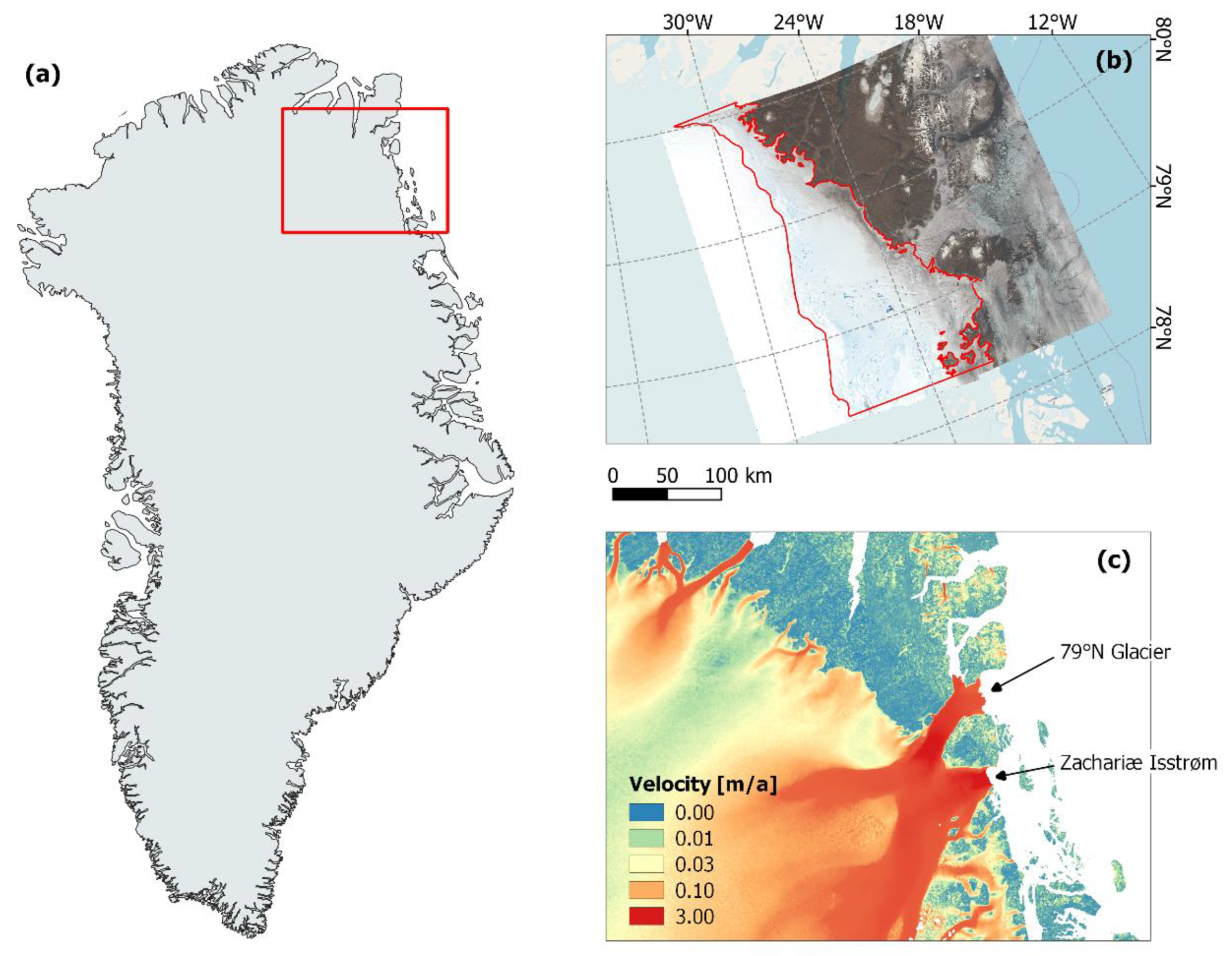
2.1. Area of Interest

This study is focused on the Nioghalvfjerdsbræ (also referred to as the 79N Glacier) and Zachariæ Isstrøm (ZI) glaciers in the Northeast Greenland Ice Stream (NEGIS), highlighted in Figure 1. This region has come to recent scientific attention, especially since the destabilization of ZI’s floating tongue and its subsequent rapid retreat [43]. These two glaciers alone drain roughly 12% of the Greenland Ice Sheet [43,44], and it is now estimated that the NEGIS region will contribute 13.5 to 15.5 mm to sea level rise by 2100 [45]. Although these glaciers are moving at a substantial rate, the SGLs on them tend to consistently develop in the same locations throughout the summer melt seasons due to the influence of the bedrock topography on the surface topography, forming local depressions on the ice surface [46,47]. The spatial area considered in this study is delineated in red in Figure 1b, comprising the ablation zone of 79N Glacier and Zachariæ Isstrøm upstream of their grounding lines, as defined in [16].

2.2. Sentinel-2 Data

The Sentinel-2 mission consists of two identical satellites that capture images containing thirteen different multispectral bands, ranging from coastal aerosol (442.7 nm) to shortwave infrared (2202.4 nm). The visible bands (red, blue and green), which are used for SGL segmentation in this study, each have a resolution of 10 m. For this analysis, Sentinel-2 A/B level-1C scenes, which provide top-of-atmosphere reflectance, are used. With the constellation’s high revisit time and polar-orbiting track, there is a roughly daily image acquisition at the latitudes used in this study. The high temporal and spatial resolution of these data allow for a nearly continuous and detailed observation of the highly dynamic processes in this region.

2.3. Data Selection and Preprocessing

There are two datasets used in this study, for different purposes: (1) algorithm development and (2) time series calculations. The data selection and preprocessing procedures for these two datasets are similar but differ in some key aspects, so they will thus be described separately.

Firstly, the dataset for algorithm development is intended to provide the deep learning algorithm with a highly diverse set of image subsections from which it can learn the characteristics and variations of the region. These images are hand-selected to ensure that different lake shapes, water colors, atmospheric conditions, shadows, and illumination conditions are present, among others. Eleven Sentinel-2 images (level 1C) were selected for this purpose and were downloaded using the Google Cloud public data repository (https://cloud.google.com/storage/docs/public-datasets/sentinel-2, accessed on 5 May 2023). The specific Sentinel-2 scenes are listed in

Table A1. The Sentinel-2 scenes used in the training and testing of the deep learning model. The number of 512 × 512 image subsets (i.e., tiles) that were used from each image are also listed.

Sentinel-2 Scene	Number of Tiles Used
S2A_MSIL1C_20160802T155912_N0204_R097_T26XNN_20160802T155907	172
S2A_MSIL1C_20170715T154911_N0205_R054_T27XVH_20170715T154905	165
S2A_MSIL1C_20200717T150921_N0209_R025_T27XVH_20200717T170914	156
S2A_MSIL1C_20210801T150911_N0301_R025_T27XVJ_20210801T171130	67
S2B_MSIL1C_20190826T153819_N0208_R011_T26XNP_20190826T191152	56
S2B_MSIL1C_20190826T153819_N0208_R011_T27XVH_20190826T191152	64
S2B_MSIL1C_20210801T155819_N0301_R097_T26XNP_20210801T175737	47
S2B_MSIL1C_20210802T152809_N0301_R111_T27XVH_20210802T173148	73
S2A_MSIL1C_20160803T152912_N0204_R111_T27XVH_20160803T152910	100
S2B_MSIL1C_20190713T155829_N0208_R097_T27XVH_20190713T193729	38
S2B_MSIL1C_20220820T153809_N0400_R011_T27XVH_20220831T150550	3

in Appendix A. These images were then tiled into subsets of 512 × 512 pixels. From these subsets, 941 were chosen to represent the wide range of surface features and their subsequent variations. A selection of these subsets can be seen in Figure 2, demonstrating the variability of these scenes. All tiles were then standardized against the training and testing dataset to fit a normal distribution.

The data for the time series evaluation, however, should consist of a series of images providing full coverage over the area of interest with as high of a temporal resolution as possible. This time series should span over an entire melt season to allow for the tracking of supraglacial lake development, using the algorithm developed in this research. Sentinel-2 scenes are available in this region from roughly mid-March to mid-September each year, allowing for complete coverage of the melt seasons. These images were filtered for scenes containing a minimum data coverage of 90%. Scenes from the same day were merged together, and then the GIMP land classification map [48], which was manually updated using a 2016 Sentinel-2 image, was used to remove non-glacier areas (e.g., rock and ocean).

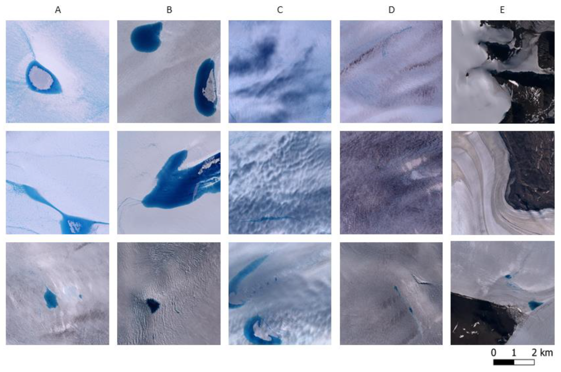
2.4. Preparation of Training and Testing Data

In order for the deep learning algorithm to learn the difference between the classes (ice, lake and rock), the training and testing data need to be labeled pixel-wise with the ground truth. As this task can be tedious to carry out manually, an online tool (segments.ai) is used to increase the efficiency of the labeling process. The output from this process is a mask (.tif) corresponding to each image subset. These image–mask pairs are then divided into the two smaller datasets, training and testing, so that the algorithm is not being tested on images that it has already seen while training. Image subsets from three Sentinel-2 scenes, totaling 141 subsets, are used for the testing dataset and eight Sentinel-2 scenes, totaling 800 subsets, are used for training, resulting in a roughly 15/85% split. While the model is being trained, a random 10% portion of the training images is set aside and used as the validation set, against which the model compares its learning after every epoch.

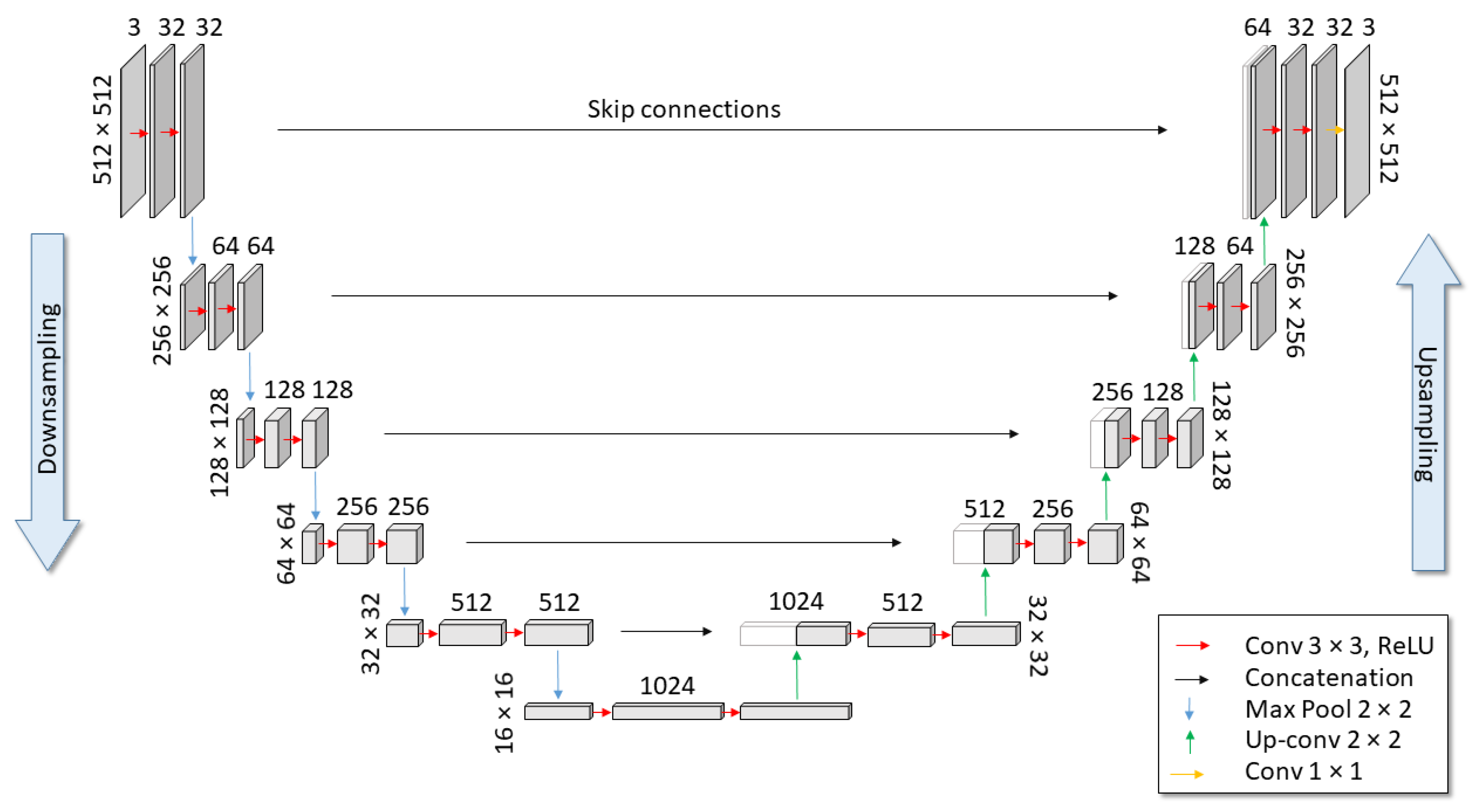
2.5. Deep Learning Architecture

A well-performing convolutional neural network for the purpose of semantic image segmentation is the U-Net architecture. Originally developed by Ronneberger et al. [49] for the purpose of biomedical image segmentation, it has proven its usefulness in many fields, including that of remote sensing. Implied by its name, the distinct feature of U-Net is its characteristic U shape, comprised of an encoder and a decoder, as shown in Figure 3, where an adapted version of U-Net is depicted. Here, the original U-Net was deepened by two extra layers in order to expand the receptive field, allowing for more spatial context for each pixel’s prediction. Initially, an image of size 512 × 512 with three visible bands (red, green, and blue) are input into the network. Indicated by the red arrows, the image then undergoes two convolutional processes, each followed by a Rectified Linear Unit (ReLU) activation function [50], increasing the amount of feature channels. Next, the image undergoes a max pooling operation to reduce the spatial dimensions. This downsampling process is continued through the encoder portion until a sufficient number of feature channels are created. The process is then reversed through the decoder portion by upsampling the data. Here, as the data is upsampled, concatenation also occurs, transferring the corresponding information from the encoder portion through skip connections, indicated by the white boxes in Figure 3. Once the image has reached its original spatial dimensions and has undergone two further convolutional processes, a final sigmoid activation function is applied to it, indicated by the orange arrow. This outputs a pixel-wise prediction, with one layer for each semantic class. Here, there are three classes: ice/snow, lake, and rock.

2.6. Model Development and Hyperparameter Tuning

This U-Net architecture is integrated into a deep learning pipeline based on Tensorflow 2.5.0 (https://www.tensorflow.org/, accessed on 5 May 2023). First, the model is compiled using a certain optimizer, loss function, and loss weights. During the model training, image and mask pairs are then fed into the network and trained over the full epoch, where the model then makes predictions on the validation data, producing an intermediate accuracy and loss value. This process is then repeated until the validation loss value has stopped improving. The total number of epochs is limited to 150, but an early stopping mechanism based on validation loss is implemented so that the model stops training before it starts overfitting to the data. The optimized model is saved and applied to the testing dataset, where various evaluation parameters are calculated. As there are many network hyperparameters that can be adjusted to produce different results, hyperparameter tuning is needed to find the optimal values. The training and testing procedure described above is repeated iteratively with the following hyperparameters over the denoted ranges or values: optimizers (Adagrad, RMS, Adam), dropout (0.0–0.4), and base learning rates (1E-6–1E-5). The loss function is always set to binary cross-entropy, and the loss weights are calculated based on the proportion of pixels assigned to each class in order to offset class bias. The performance of each model on the testing dataset are then compared, and the model with the highest Cohen’s kappa and F1-scores is selected.

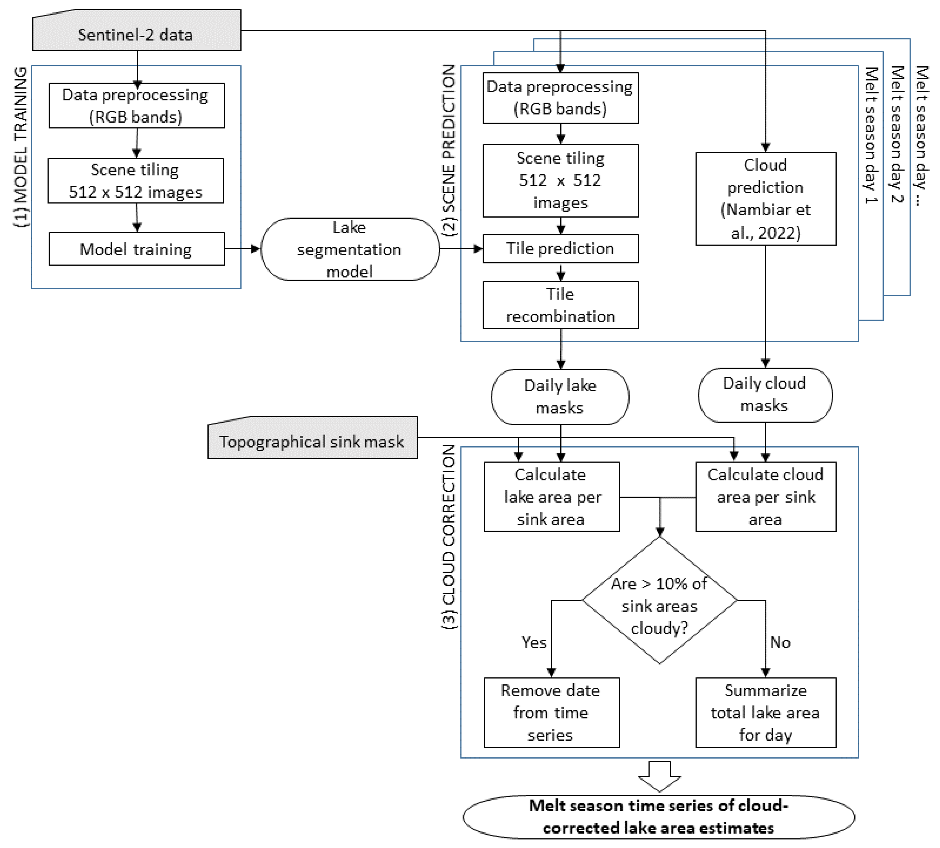
2.7. Post-Processing and Time Series Evaluation

Having completed the deep learning model development phase, the model is then applied to the image time series over the full melt season. First, each image is segmented into tiles of 512 × 512 pixels for computational efficiency before the standardization scaler created from the training process is applied. Then, the model first makes a prediction to each tile before merging the scene back together, producing an array containing one layer per semantic class. Each pixel in this array represents the probability that this pixel belongs to a certain class. Thus, to determine the prediction, the class with the highest probability is chosen for each pixel. Then, the closing morphological function is applied to the prediction to fill in small gaps and smooth out edges. Finally, the prediction arrays are converted to vectors and saved as a shapefile.

In order to track specific lake development over the melt season, it is necessary to assign IDs to different lakes. As mentioned previously, supraglacial lakes tend to form in roughly the same positions every year, due to the fact that there are surface depressions on the glacier’s surface that are formed by the topography of the bedrock [46]. These topographic sinks have been mapped out for this region using ArcticDEM in the process described in [16]. Any lakes that have formed within the boundary of a topographic sink or within 300 m of one are assigned to that sink’s ID, and the lake area is then calculated.

An important component of the development of a supraglacial-lake-area time series is the ability to identify when clouds are covering the region. For this, we use the newly developed deep learning-based cloud segmentation algorithm from Nambiar et al. [42], which was trained specifically for cloud segmentation over polar regions. This model takes the raw Sentinel-2 scenes as input and outputs a raster prediction. The model uses all 13 spectral bands, since the distinction between clouds and ice/snow cover is particularly difficult using visible bands alone. The cloud predictions from the same day are then merged to provide the same spatial coverage as the merged Sentinel-2 scenes on which the lake predictions are made.

Using both the lake-area masks and the cloud masks, a cloud coverage identification and correction procedure is able to be implemented for each scene, as indicated in Figure 4. For each topographic sink, the percentage of cloud-covered area is calculated. If more than 10% of the total amount of sink area (i.e., hypothetical lake area) is covered by clouds, the image from the corresponding day is removed from the time series. After this cloud check is conducted over the entire melt season, the total lake-area trend can be seen for each year.

3. Results

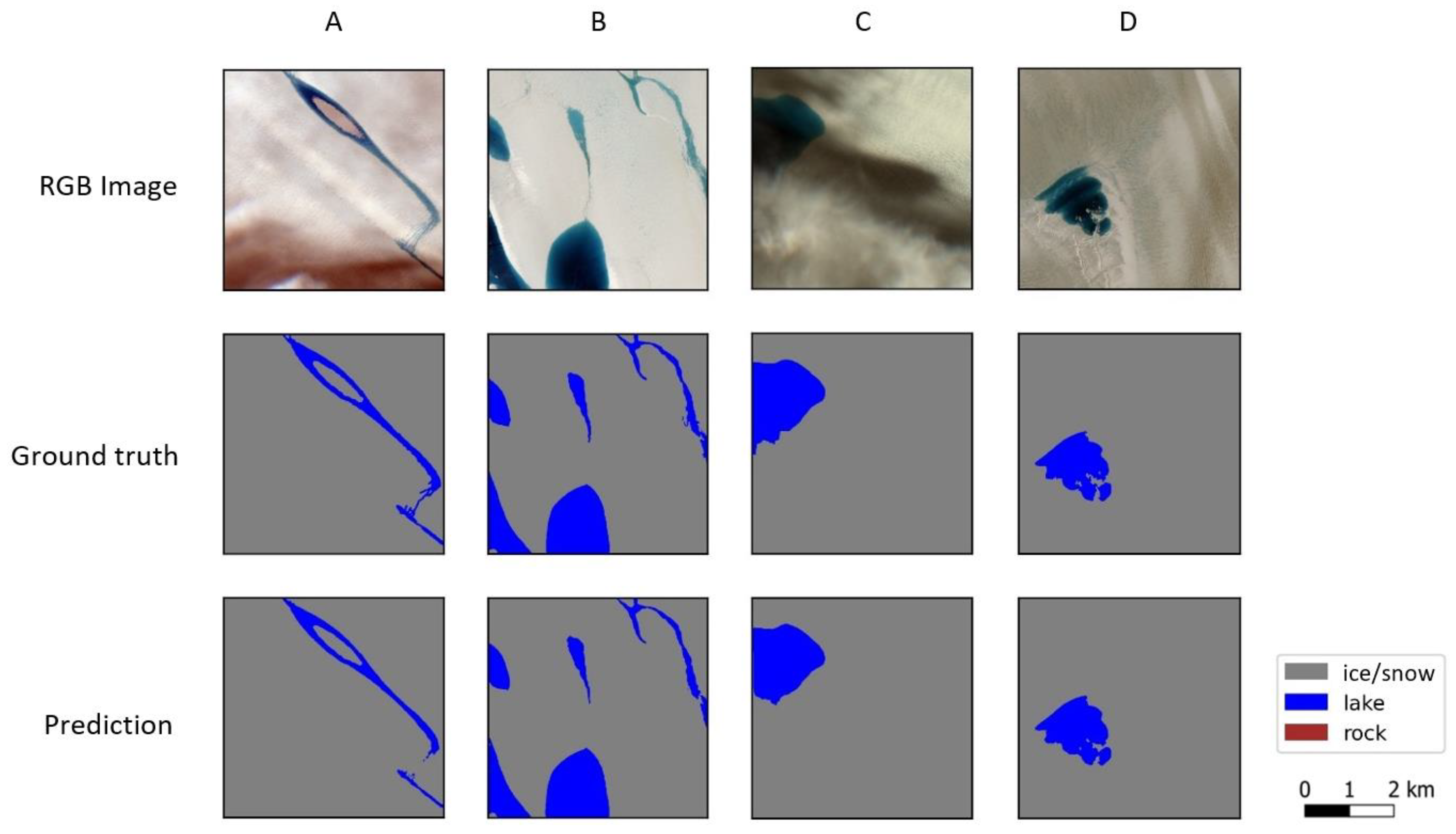
3.1. Model Selection and Application to Testing Dataset

During the hyperparameter trials conducted to determine the best deep learning model, different performance metrics are calculated and compared. Since the testing dataset has a strong class imbalance, with the majority of pixels being assigned to the class ice/snow, the use of accuracy as the primary evaluator is misleading and limiting to model improvement. Thus, several other metrics, such as precision, recall, F1-score and Cohen’s kappa coefficient, are calculated to provide more insight into the model’s performance. Since Cohen’s kappa coefficient is able to counteract class imbalance skew while providing a single value across classes, it was used as the main factor for determining a model’s success.

The best performing model was accordingly selected, containing the following hyperparameters: dropout (0.0), learning rate (0.000005) and optimizer (Adam). The performance metrics of this model are listed in

Table 1. Performance metrics of the selected deep learning model applied to the testing data.

Class	Precision	Recall	F1-Score	Accuracy	Kappa Coefficient
Ice/snow	1.00	1.00	1.00	0.99	0.93
Lake	0.90	0.91	0.90
Rock	0.98	0.92	0.95

. These metrics are calculated based on a diverse testing dataset, as outlined in Section 2.3. The metrics for all three classes are relatively high (i.e., above 0.90) with the lake class scoring lowest, primarily due to false-negative classifications around some lake edges and some false-positive classifications over rock and very dark shadows.

In Figure 5, four example testing images are shown, along with their manually derived ground-truth labels and the prediction labels from the model. In general, the prediction labels tend to follow the lake contours rather precisely, with only small areas of false negatives and positives. Additionally, since existing supraglacial lake segmentation algorithms tend to falsely identify shadows on ice as lakes, the testing dataset was created with a significant percentage of images containing shadows (19.15% of the entire testing dataset). Two of these images are shown here in columns A and C, demonstrating the model’s ability to differentiate between lake and shadow. Furthermore, out of all the testing images containing shadow, only three contained portions of falsely classified shadows.

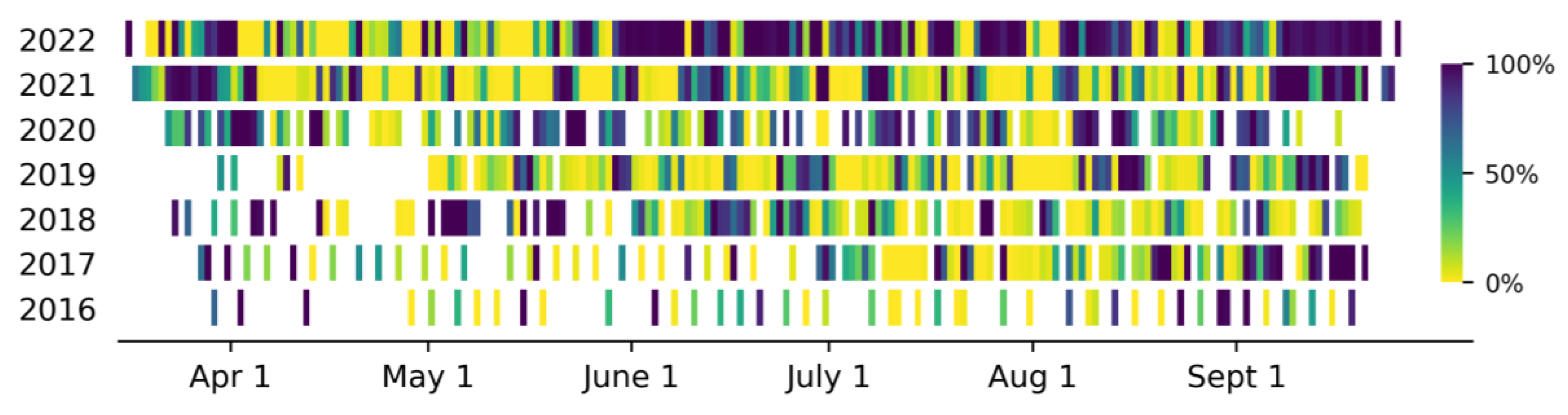
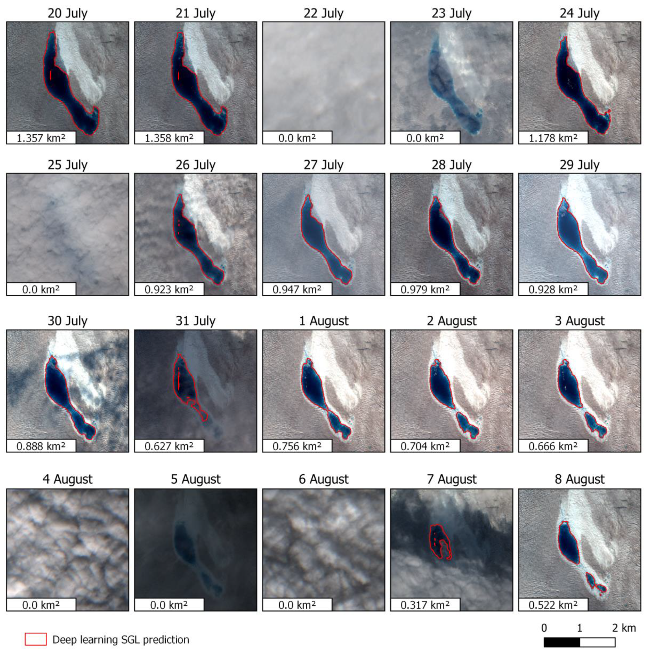
3.2. Influence of Cloudy Days on Time Series Results

As a result of the application of the cloud segmentation algorithm over the time series, an evaluation of the daily cloud cover could be made. While the cloud segmentation algorithm worked quite well in general, some manual adjustments were needed for the early 2022 melt season. Figure 6 shows a daily cloud percentage calculated over the topographic sink areas, i.e., the locations where lakes could potentially form. Here, yellow represents a cloud-free day and dark blue depicts a day where all sink areas were completely covered by clouds. Days with insufficient Sentinel-2 data are depicted in white. As cloud coverage is dependent on the variable local weather system, there is not an interannual trend to be seen. An interesting point, however, is the persistent stretches of full cloud coverage in 2022. The number of cloud-free days is also relatively sparse in 2020; however, there are fewer days of complete cloud coverage, in contrast to 2022. The percentage of days with at least 20% cloud coverage are shown in

Table 2. Number of days in each melt season (15 March to 30 September) where at least 20% of the potential lake areas are covered by clouds.

	2016	2017	2018	2019	2020	2021	2022
Number of cloudy days (out of total images *)	20/52	27/100	42/137	51/176	68/110	73/168	114/179
Percentage of cloudy days	38.5%	27.0%	30.7%	32.4%	61.8%	43.5%	63.7%

* Some years contain fewer images due to lack of available data coverage of the entire area of interest, particularly in the earlier years of Sentinel-2′s operation.

, where it can be seen that the percentages for these two years are roughly equivalent. In comparison, 2019 had a relatively cloud-free melt season, with only 32% of the available images containing more than 20% cloud coverage over the lakes.

The importance of accurate cloud masks is demonstrated in Figure 7, where the time series of an example lake over a 20-day period in 2021 is shown. These daily images show the segmentation of the lake boundary from the deep learning model as well as the estimated lake area in the lower left corner. There are six days in which clouds or cloud shadows fully inhibit the identification of the lake boundary. Furthermore, there are two days, 31 July and 7 August, where only a portion of the lake is segmented due to partial cloud coverage. Without the removal of both the fully and partially cloud-covered days, the lake-area time series would appear very jumpy and it would be more difficult to determine where the actual trend lies. Figure 7 also demonstrates how dynamic an SGL can be. In less than three weeks, this lake decreases in area by roughly 62%, causing the lake to separate into three disconnected bodies of water.

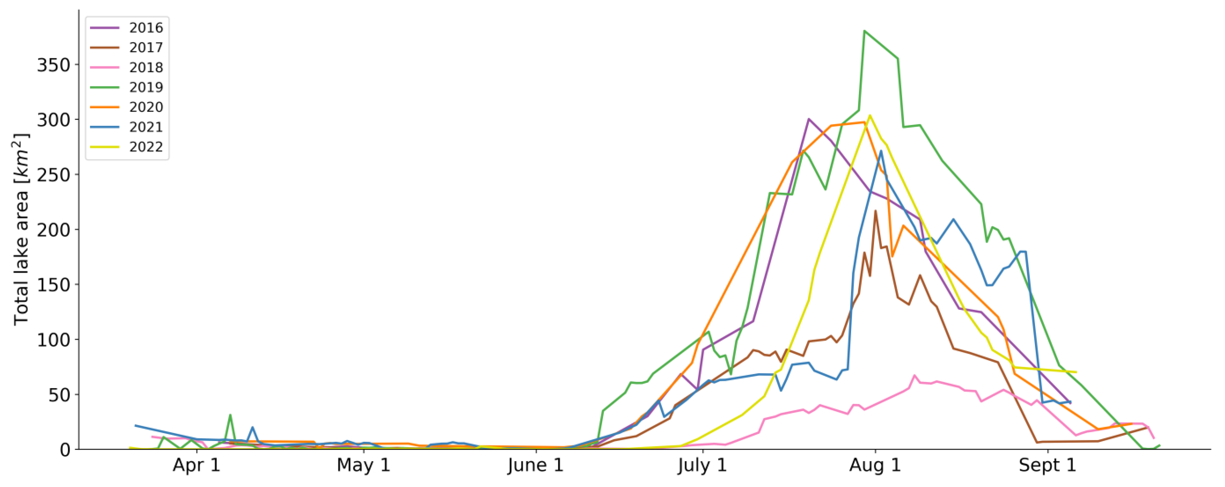
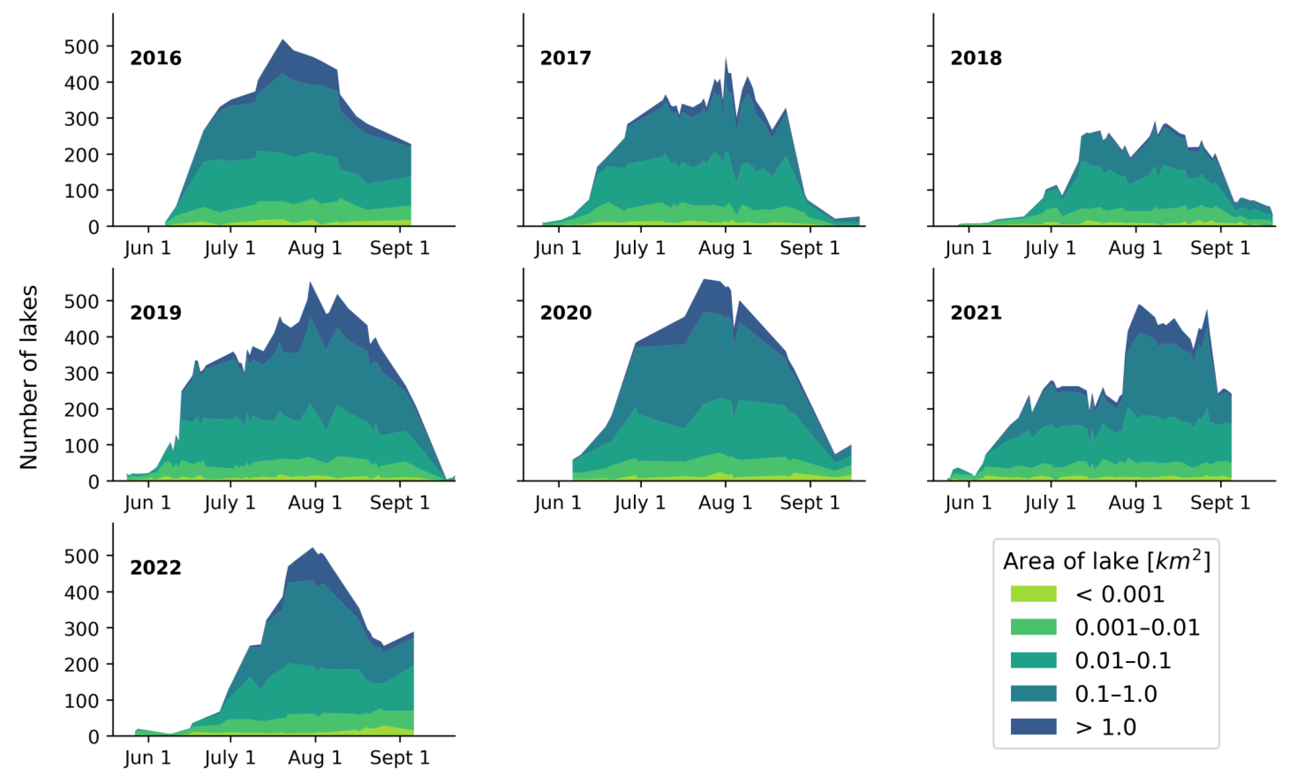
3.3. Seasonal Trends and Interannual Comparison of Supraglacial Lake Area

The results from the time series calculations can be seen in Figure 8, where the daily total lake area is tracked over the entire melt season for the years 2016 to 2022. In general, each melt season follows a similar trend, reaching the peak lake area around 1 August. The development progression and quantity of meltwater, however, vary strongly among the years. For example, the peak lake area for 2019 is roughly 5.6× the amount of that in 2018, due to drastically different local weather conditions, as investigated by Turton et al. [2]. Additionally, while most years begin showing significant lake development in early June, this is not apparent until early July in 2022. Furthermore, the threshold for acceptable cloud coverage was raised to 20% for 2022 (from the 10% used for the other years), due to an insufficient number of cloud-free days during the peak of the melt season.

While the model performed well as a whole over the time series, there were a couple of situations for which manual adjustments were needed. Firstly, in the peak of some melt seasons, the amount of meltwater is so high that the ice and snow surface itself turns a light blue, seemingly due to some form of stagnant surface melt or slush. These areas appear to be very shallow, but can be widespread, causing a sudden and drastic increase in detected lake area. As this is an unrepresentative depiction of the seasonal lake-area development, these days (totaling 2 days in 2016, 5 days in 2019, 1 day in 2020, and 2 days in 2021) were removed from the time series. Secondly, even though the majority of cloud shadows were ignored by the model, there were three instances of large, very dark cloud shadows being falsely included in the lake-area estimation. These areas were removed from the daily lake-area total to ensure a trend more reflective of the actual lake area.

Figure 9 shows the evolution of the number of SGLs and their size distribution over the 2016 to 2022 melt seasons. The lakes were sorted into five bins based on their area, where the smallest lakes (<0.001 km²) are represented by light green and the largest lakes (>1.0 km²) are represented by dark blue. Each bin is stacked upon the previous one, cumulating in the total number of lakes. Thus, the height of each color represents the number of lakes in the respective bin. For most years, a similar maximum number of lakes can be seen, with an average of 520 lakes, excluding the 2018 melt season, which only reached a maximum of 294 lakes. This information, along with details about the average lake size on peak days, can be found in

Table 3. The maximum number of lakes recorded per melt season, the date upon which it was recorded, and the average lake area on that day with the associated standard deviation (km²).

	2016	2017	2018	2019	2020	2021	2022
Date of maximum number of lakes	20 July	1 August	8 August	30 July	24 July	2 August	3 August
Maximum number of lakes	424	472	294	555	561	491	508
Average lake area on peak date (km2)	1.24 ± 3.52	0.57 ± 1.25	0.23 ± 0.48	1.06 ± 2.94	0.57 ± 1.33	0.70 ± 1.61	0.80 ± 2.65

. Here, it can be seen that the average lake size varies quite drastically among the melt seasons. Furthermore, as expected, the day on which the peak number of lakes occurs tends to coincide with the maximum total lake area for each melt season.

It can also be seen in Figure 9 that the number of lakes within each bin tends to saturate after a certain threshold, after which lakes of a larger size begin developing. This can be visually seen by the plateau in each bin throughout the central part of the melt seasons. Averaging over all melt seasons, these thresholds were found to be 11.4 ± 2.1 lakes, 42.3 ± 4.4 lakes, 122.1 ± 11.6 lakes, and 190.8 ± 23.2 lakes for lakes smaller than 0.001 km², between 0.001 and 0.01 km², between 0.01 and 0.1 km², and between 0.1 and 1.0 km², respectively. The 2018 melt season was excluded from the calculations of the final threshold (lakes between 0.1 and 1.0 km²) since very few lakes achieved a size larger than 1.0 km². This pattern implies that a stable point is reached throughout the melt seasons, where new lakes begin appearing at the same rate that existing lakes grow in size. This thus causes the lower bins to remain at a relatively fixed size, while the uppermost bin(s) continue to grow.

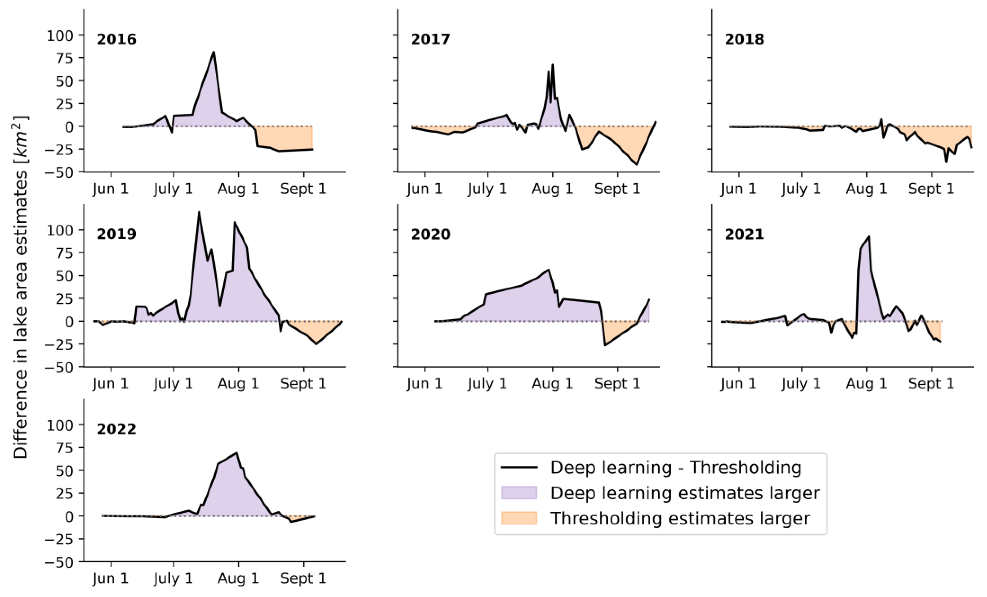
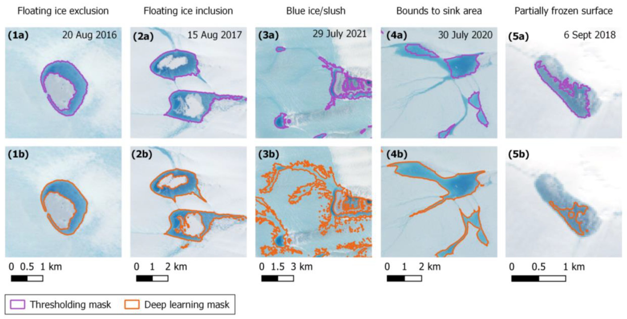
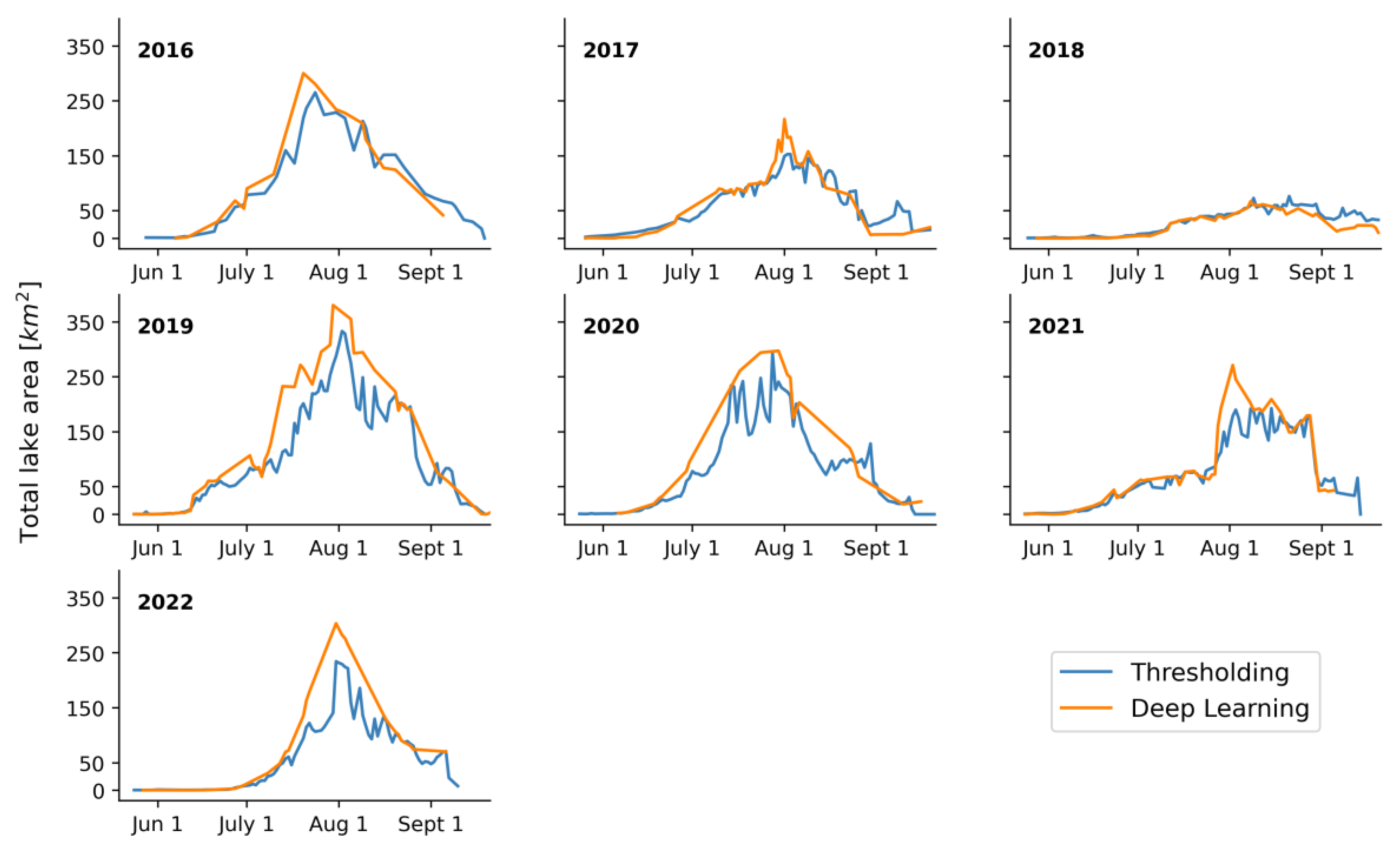
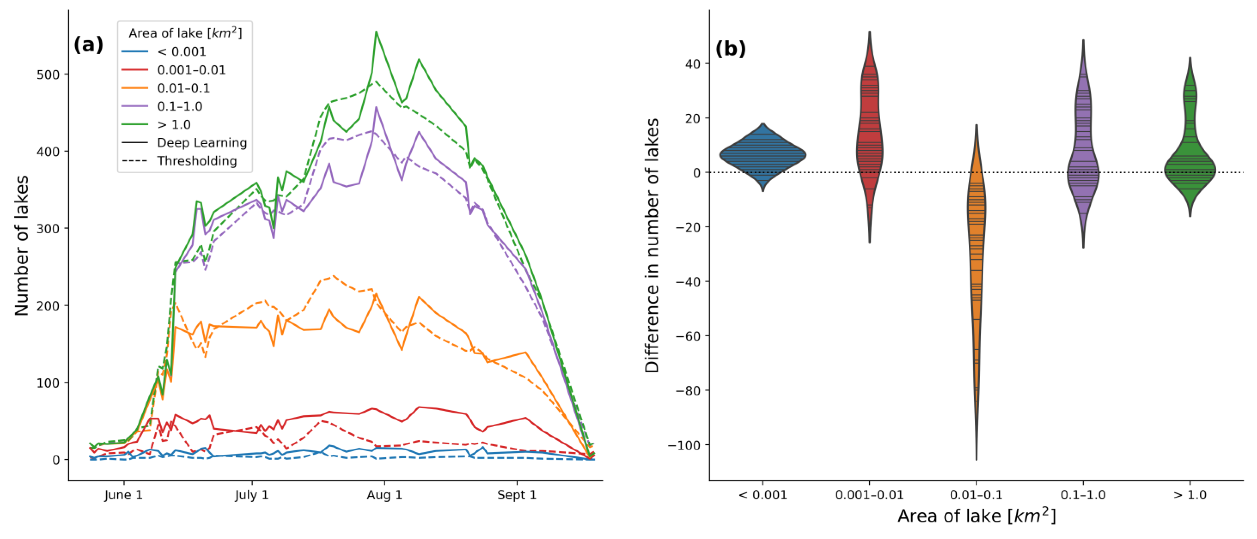
3.4. Comparison between Methods: Thresholding vs. Deep Learning

To benchmark the use of this deep learning model for SGL segmentation, the method used by Hochreuther et al. [16], in which the red and blue bands are used to create a lake threshold, was extended to cover the same temporal span as the time series in this study. As both studies use the same images and cover the same spatial extent, the distinction between the results is purely based on the methodology.

Table 4. Comparison of the maximum total lake area over the area of interest using the thresholding method extended from [16] and the deep learning method developed in this study.

	2016	2017	2018	2019	2020	2021	2022
Peak lake area from thresholding method (km2)	265.39	153.26	76.66	333.19	292.91	192.83	234.30
Peak lake area from deep learning method (km2)	300.33	184.47	67.27	380.47	297.47	271.41	303.67

shows the peak total lake area achieved throughout the melt season for each methodology. Here, it can be seen that the peak areas for both methods are on the same scale and are of a relatively similar size compared to other years. The main difference is that the deep learning method consistently has a significantly higher peak lake area, with the exception of 2018 and 2020.

A more detailed look at the time series created by each method is provided in Figure 10. For each melt season, the results from each method generally follow similar trends, with coinciding timings for lake growth and shrinkage. The main differences generally come from three sources. Firstly, the quality of the cloud-masking algorithm strongly influences the smoothness of the time series. The algorithm used in the thresholding method was statistically based, and while it removed days with complete cloud coverage well, it seems to have included many days of partial cloudiness, resulting in much jumpier results. The deep learning method, in contrast, removed scenes with a much smaller cloud presence. Thus, misinterpretation of this jumpiness is avoided in the deep learning method. The second source of difference between the time series is the generally larger lake-area estimations provided by the deep learning method. This stems from a difference in definition of where lakes can develop. In the thresholding method, lake area was restricted to only occurring within the boundaries of the predefined sink areas; any area falling outside was not counted as part of a lake. Contrarily, this definition was more relaxed in the deep learning processing chain. Here, the sink areas were used to assign IDs to the bodies of water, but the lakes were not purely limited to the sink areas; any body of water coming at some point within 300 m of a sink was assigned to that sink. This allows for more water to be counted towards the lakes and generally increases the amount of lake area estimated by the deep learning algorithm. This is particularly prominent during periods of higher melt, when the meltwater tends to exceed the extent of the sink areas. The final main source of difference between the estimates originates in a post-processing step included in the thresholding method. In an attempt to include floating ice into the lake area, the thresholding method aggregates the floating-ice area if it is completely surrounded by lake water pixels. Otherwise, if even a pixel of the floating ice is in contact with the edge of the lake, the entire floating-ice area is excluded from the estimation. Since such a processing step does not exist in the deep learning method, periods of time where floating ice is found in the center of a lake have a higher total lake-area estimation for the thresholding method. Examples of this can be seen later in the 2016, 2017, and 2018 melt seasons. One additional minor source of discrepancy between the methods lies with the freezing of the lakes at the end of the melt season. As the lakes begin to freeze over in September, both methods tend to give inconsistent results as the color becomes lighter and less homogeneous. The thresholding method tends to continue including portions of the frozen lake, while the deep learning method includes a bit less. These differences are relatively minimal, but are nonetheless a factor in the discrepancy. A more direct look at the differences between the two methods can be seen in Figure A1 in Appendix A. Additionally, examples of floating-ice inclusion and exclusion, along with the limitation of the thresholding method to the sink areas, are shown in Figure A2 in Appendix A.

In Figure 11, the differences between the two methods are further investigated by analyzing the distribution of lake sizes over the melt season. Figure 11a displays a cumulative plot of the number of lakes found in each bin for both methods over the 2019 melt season. Here, the colors represent the five categories based on area, where the smallest lakes (<0.001 km²) are represented by blue and the largest lakes (>1.0 km²) are represented by green. It can be seen that while the general trends are similar for each method, there are significant differences in the number of lakes found in each bin. These differences are further highlighted in Figure 11b, where the differences between the methods were calculated each day for each bin. Positive differences indicate that the deep learning method has found more lakes than the thresholding method in that category of lake sizes. Four of the categories have positive averages, with the majority of data points falling above zero. One category, however, almost entirely falls in the negative range, indicating that the thresholding method has found more lakes of this size (0.01–0.1 km²). The two categories for the smallest lakes (<0.001 km² and 0.001–0.01 km²) have average differences of 4.3 and 10.6, respectively. Almost every data point for these categories shows a significantly larger number of lakes found by the deep learning model. This implies that the deep learning model was either (1) better at detecting smaller lakes, and/or (2) it was detecting smaller portions of medium-sized lakes than the thresholding method. This second point is more likely for areas of mixed pixels found around lake boundaries, in particularly during periods of refreezing, an example of which is shown in Figure A2 in Appendix A. The two largest categories (0.1–1.0 km² and >1.0 km²) tend to have more days with minimal differences in the number of lakes, as seen by the larger bulges around zero in Figure 11b. There are, however, also days on which the difference is quite large. This is primarily influenced by the deep learning method’s inclusion of more and larger lakes during the peak melt season. This effect is additionally seen by the significant negative differences found in the category of 0.01–0.1 km², with an average difference of −14.1. The larger number of these medium-sized lakes for the thresholding method compensate for the smaller number of larger lakes present in the other categories.

4. Discussion

As seen with other remote sensing applications, deep learning techniques have proven to be capable of accomplishing tasks comparably well when compared to traditional methods. That is not to say, however, that the method development phases are equal in terms of effort and straightforwardness or that the results are identical. While traditional methods, such as thresholding techniques, generally have the challenge of inadaptability and require the direct definition of many conditions to eliminate undesirable inclusions in the results, deep learning methods have their own challenges. Firstly, the preparation of ground-truth labels for the training and testing images is quite tedious and time-consuming. Furthermore, even though the principles of training the model and tuning the hyperparameters are relatively basic, the outcome is not directly controllable by the user, rendering it difficult to curate desirable results without running a significant number of grid-search trials.

The quality of the results of the two methods brings forth another point of discussion. As mentioned previously, proper cloud segmentation plays a significant role in the smoothness and accurate representation of the state of meltwater on the surface. However, even if both the thresholding and deep learning techniques used the same high-quality cloud segmentation algorithm, there would still be differences in the results. The limitation of the predictions to the predefined sink areas in the thresholding method has the benefit of outputting consistent results, largely free from false-positive segmentations. Even though this limits the inclusion of meltwater that accumulates outside of these areas, this is necessary because of the otherwise widespread inclusion of false positives such as cloud shadows. With the deep learning method, the results do not need to be constrained to certain areas because the algorithm has been trained not to include shadows in the results, for the most part. Thus, the deep learning model is able to include more meltwater in the lake-area estimation than the thresholding method. It is also less sensitive to a changing ice geometry than the thresholding algorithm, and is hence better suited for fast changing areas of the Greenland Ice Sheet.

While the deep learning model performed quite well in this study, there are still areas in which it could be improved. As mentioned previously, during the peak of a heavy melt season, the model tends to include widespread, thin layers of meltwater or slush appearing across the ice surface. An example of this can be seen in Figure A2 in Appendix A. The model was never presented with images containing surface conditions like this during training, so it rather inconsistently includes these areas when they are present. To improve the model, images containing this kind of slush should be added into the training and defined as either something that should or should not be marked as supraglacial lakes, for a more consistent prediction. The difficulty therein, however, lies with one’s ability to be able to distinguish where these zones concretely start and end to be able to properly teach the model which areas belong to the ice sheet and which to the lakes. Furthermore, even though an intentional effort was directed into including shadows in the training dataset in order to avoid misclassifications, there were still a few instances of false positives due to shadows. The majority of cloud shadows were properly avoided; however, a few really dark ones were falsely classified. Similarly, at the beginning and end of the polar summer (i.e., March and September), the sun is so low on the horizon that large shadows are cast on the ice from the surrounding rock outcroppings. These shadows are very dark and it is difficult for even the human eye to distinguish whether they are lakes or shadows. Consequently, these topographic shadows were falsely classified as lakes in March and the beginning of April, which can be seen by the slight upturn in lake area in Figure 8. Considering that the misclassification of shadows has been a ubiquitous problem in this field until now, the capabilities shown through deep learning in this study demonstrates a potential for eradicating at least a significant portion of them. Finally, as the inclusion of floating ice is not addressed by the deep learning approach, the geospatial post-processing step used in the thresholding method could be integrated with the deep learning pipeline to allow additional lake area to be included. While this processing step does not lead to consistent floating-ice inclusion, it provides a basis for floating-ice area estimations.

5. Conclusions

In this study, the capabilities of deep learning for the purpose of supraglacial lake segmentation in multispectral images have been demonstrated. Here, a deep learning pipeline based on the U-Net architecture has been implemented and applied to Sentinel-2 images throughout the 2016 to 2022 melt seasons. While there are still aspects of this method that occasionally lead to false-positive detections, a comprehensive and relatively consistent product is able to be generated. Furthermore, this model’s areas of weakness could be improved upon by including more training data tailored to specific situations, e.g., very dark shadows and slushy-snow and ice surfaces. Additionally, these results have been compared to a standard red/blue thresholding technique, highlighting the congruence of the results produced from the two differing methodologies, as well as the areas upon which deep learning improves the output. Lastly, the importance of an accurate cloud segmentation algorithm for the development of a smooth time series is highlighted.

There are several related topics that would be interesting to explore in future research. Firstly, the model in this study was trained and applied only on images procured over the NEGIS region. Further analysis would be needed to be able to determine if this model would be able to be seamlessly transferred to other areas in Greenland or even Antarctica, or if the model would need to be adjusted. Furthermore, with relatively accurate cloud and lake-segmentation algorithms, it would be possible to apply them to create a rapid drainage detection algorithm. The automated detection of such drainages would be advantageous for investigating their cause and their influence on surface and subglacial hydrology. Additionally, the implementation of a comparison study to evaluate the effectiveness of different deep learning techniques would be advantageous in order to determine the network optimally suited for the task. Finally, while the quantification of lake area is an important first step in understanding the dynamics of surface meltwater, the corresponding volume would bring an even deeper understanding and would allow for incorporation of these values into hydrological and climate models. Overall, this study provides a confirmation of the applicability of machine learning to remote sensing topics and also provides context for its strengths and weaknesses.

References

1. Oppenheimer, M.; Glavovic, B.C.; Hinkel, J.; van de Wal, R.; Magnan, A.K.; Abd-Elgawad, A.; Cai, R.; Cifuentes-Jara, M.; DeConto, R.M.; Ghosh, T.; et al. Sea level rise and implications for low-lying islands, coasts and communities. In IPCC Special Report on the Ocean and Cryosphere in a Changing Climate; Pörtner, H.-O., Roberts, D.C., Masson-Delmotte, V., Zhai, P., Tignor, M., Poloczanska, E., Mintenbeck, K., Alegría, A., Nicolai, M., Okem, A., et al., Eds.; Cambridge University Press: Cambridge, UK, 2022; pp. 321–446. ISBN 9781009157964. [Google Scholar]
2. Turton, J.; Hochreuther, P.; Reimann, N.; Blau, M. The distribution and evolution of supraglacial lakes on the 79° N Glacier (northeast Greenland) and interannual climatic controls. Cryosphere Discuss. 2021, 15, 3877–3896. [Google Scholar] [CrossRef]
3. Lüthje, M.; Pedersen, L.T.; Reeh, N.; Greuell, W. Modelling the evolution of supraglacial lakes on the west Greenland ice-sheet margin. J. Glaciol. 2006, 52, 608–618. [Google Scholar] [CrossRef]
4. Tedesco, M.; Steiner, N. In-situ multispectral and bathymetric measurements over a supraglacial lake in western Greenland using a remotely controlled watercraft. Cryosphere 2011, 5, 445–452. [Google Scholar] [CrossRef]
5. Bartholomew, I.; Nienow, P.; Sole, A.; Mair, D.; Cowton, T.; Palmer, S.; Wadham, J. Supraglacial forcing of subglacial drainage in the ablation zone of the Greenland ice sheet. Geophys. Res. Lett. 2011, 38, L08502. [Google Scholar] [CrossRef]
6. Doyle, S.H.; Hubbard, A.L.; Dow, C.F.; Jones, G.A.; Fitzpatrick, A.; Gusmeroli, A.; Kulessa, B.; Lindback, K.; Pettersson, R.; Box, J.E. Ice tectonic deformation during the rapid in situ drainage of a supraglacial lake on the Greenland Ice Sheet. Cryosphere 2013, 7, 129–140. [Google Scholar] [CrossRef]
7. Zwally, H.J.; Abdalati, W.; Herring, T.; Larson, K.; Saba, J.; Steffen, K. Surface melt-induced acceleration of Greenland ice-sheet flow. Science 2002, 297, 218–222. [Google Scholar] [CrossRef] [PubMed]
8. Das, S.B.; Joughin, I.; Behn, M.D.; Howat, I.M.; King, M.A.; Lizarralde, D.; Bhatia, M.P. Fracture Propagation to the Base of the Greenland Ice Sheet During Supraglacial Lake Drainage. Science 2008, 320, 778–781. [Google Scholar] [CrossRef]
9. Danielson, B.; Sharp, M. Development and application of a time-lapse photograph analysis method to investigate the link between tidewater glacier flow variations and supraglacial lake drainage events. J. Glaciol. 2013, 59, 287–302. [Google Scholar] [CrossRef]
10. Chudley, T.R.; Christoffersen, P.; Doyle, S.H.; Bougamont, M.; Schoonman, C.M.; Hubbard, B.; James, M.R. Supraglacial lake drainage at a fast-flowing Greenlandic outlet glacier. Proc. Natl. Acad. Sci. USA 2019, 116, 25468–25477. [Google Scholar] [CrossRef]
11. Neckel, N.; Zeising, O.; Steinhage, D.; Helm, V.; Humbert, A. Seasonal Observations at 79° N Glacier (Greenland) From Remote Sensing and in situ Measurements. Front. Earth Sci. 2020, 8, 142. [Google Scholar] [CrossRef]
12. Wessels, R.L.; Kargel, J.S.; Kieffer, H.H. ASTER measurement of supraglacial lakes in the Mount Everest region of the Himalaya. Ann. Glaciol. 2002, 34, 399–408. [Google Scholar] [CrossRef]
13. Box, J.E.; Ski, K. Remote sounding of Greenland supraglacial melt lakes: Implications for subglacial hydraulics. J. Glaciol. 2007, 53, 257–265. [Google Scholar] [CrossRef]
14. Banwell, A.F.; Caballero, M.; Arnold, N.S.; Glasser, N.F.; Cathles, L.M.; MacAyeal, D.R. Supraglacial lakes on the Larsen B ice shelf, Antarctica, and at Paakitsoq, West Greenland: A comparative study. Ann. Glaciol. 2014, 55, 1–8. [Google Scholar] [CrossRef]
15. Pope, A.; Scambos, T.A.; Moussavi, M.; Tedesco, M.; Willis, M.; Shean, D.; Grigsby, S. Estimating supraglacial lake depth in West Greenland using Landsat 8 and comparison with other multispectral methods. Cryosphere 2016, 10, 15–27. [Google Scholar] [CrossRef]
16. Hochreuther, P.; Neckel, N.; Reimann, N.; Humbert, A.; Braun, M. Fully automated detection of supraglacial lake area for northeast greenland using sentinel-2 time-series. Remote Sens. 2021, 13, 205. [Google Scholar] [CrossRef]
17. Everett, A.; Murray, T.; Selmes, N.; Rutt, I.C.; Luckman, A.; James, T.D.; Clason, C.; O’Leary, M.; Karunarathna, H.; Moloney, V.; et al. Annual down-glacier drainage of lakes and water-filled crevasses at Helheim Glacier, southeast Greenland. J. Geophys. Res. Earth Surf. 2016, 121, 1819–1833. [Google Scholar] [CrossRef]
18. Williamson, A.G.; Arnold, N.S.; Banwell, A.F.; Willis, I.C. A Fully Automated Supraglacial lake area and volume Tracking (“FAST”) algorithm: Development and application using MODIS imagery of West Greenland. Remote Sens. Environ. 2017, 196, 113–133. [Google Scholar] [CrossRef]
19. Stokes, C.R.; Sanderson, J.E.; Miles, B.W.J.; Jamieson, S.S.R.; Leeson, A.A. Widespread distribution of supraglacial lakes around the margin of the East Antarctic Ice Sheet. Sci. Rep. 2019, 9, 13823. [Google Scholar] [CrossRef]
20. Yang, K.; Smith, L.C. Supraglacial Streams on the Greenland Ice Sheet Delineated from Combined Spectral–Shape Information in High-Resolution Satellite Imagery. IEEE Geosci. Remote Sens. Lett. 2013, 10, 801–805. [Google Scholar] [CrossRef]
21. Miles, K.E.; Willis, I.C.; Benedek, C.L.; Williamson, A.G.; Tedesco, M. Toward Monitoring Surface and Subsurface Lakes on the Greenland Ice Sheet Using Sentinel-1 SAR and Landsat-8 OLI Imagery. Front. Earth Sci. 2017, 5, 58. [Google Scholar] [CrossRef]
22. Williamson, A.G.; Banwell, A.F.; Willis, I.C.; Arnold, N.S. Dual-satellite (Sentinel-2 and Landsat 8) remote sensing of supraglacial lakes in Greenland. Cryosphere 2018, 12, 3045–3065. [Google Scholar] [CrossRef]
23. Arthur, J.F.; Stokes, C.R.; Jamieson, S.S.; Carr, J.R.; Leeson, A.A. Distribution and seasonal evolution of supraglacial lakes on Shackleton Ice Shelf, East Antarctica. Cryosphere 2020, 14, 4103–4120. [Google Scholar] [CrossRef]
24. Carrivick, J.L.; Quincey, D.J. Progressive increase in number and volume of ice-marginal lakes on the western margin of the Greenland Ice Sheet. Glob. Planet. Change 2014, 116, 156–163. [Google Scholar] [CrossRef]
25. Shugar, D.H.; Burr, A.; Haritashya, U.K.; Kargel, J.S.; Watson, C.S.; Kennedy, M.C.; Bevington, A.R.; Betts, R.A.; Harrison, S.; Strattman, K. Rapid worldwide growth of glacial lakes since 1990. Nat. Clim. Change 2020, 10, 939–945. [Google Scholar] [CrossRef]
26. Moussavi, M.; Pope, A.; Halberstadt, A.; Trusel, L.D.; Cioffi, L.; Abdalati, W. Antarctic Supraglacial Lake Detection Using Landsat 8 and Sentinel-2 Imagery: Towards Continental Generation of Lake Volumes. Remote Sens. 2020, 12, 134. [Google Scholar] [CrossRef]
27. Schröder, L.; Neckel, N.; Zindler, R.; Humbert, A. Perennial Supraglacial Lakes in Northeast Greenland Observed by Polarimetric SAR. Remote Sens. 2020, 12, 2798. [Google Scholar] [CrossRef]
28. Benedek, C.L.; Willis, I.C. Winter drainage of surface lakes on the Greenland Ice Sheet from Sentinel-1 SAR imagery. Cryosphere 2021, 15, 1587–1606. [Google Scholar] [CrossRef]
29. Li, W.; Lhermitte, S.; López-Dekker, P. The potential of synthetic aperture radar interferometry for assessing meltwater lake dynamics on Antarctic ice shelves. Cryosphere 2021, 15, 5309–5322. [Google Scholar] [CrossRef]
30. Halberstadt, A.R.W.; Gleason, C.J.; Moussavi, M.S.; Pope, A.; Trusel, L.D.; DeConto, R.M. Antarctic Supraglacial Lake Identification Using Landsat-8 Image Classification. Remote Sens. 2020, 12, 1327. [Google Scholar] [CrossRef]
31. Wangchuk, S.; Bolch, T. Mapping of glacial lakes using Sentinel-1 and Sentinel-2 data and a random forest classifier: Strengths and challenges. Sci. Remote Sens. 2020, 2, 100008. [Google Scholar] [CrossRef]
32. Yuan, J.; Chi, Z.; Cheng, X.; Zhang, T.; Li, T.; Chen, Z. Automatic Extraction of Supraglacial Lakes in Southwest Greenland during the 2014–2018 Melt Seasons Based on Convolutional Neural Network. Water 2020, 12, 891. [Google Scholar] [CrossRef]
33. Dirscherl, M.; Dietz, A.J.; Kneisel, C.; Kuenzer, C. Automated Mapping of Antarctic Supraglacial Lakes Using a Machine Learning Approach. Remote Sens. 2020, 12, 1203. [Google Scholar] [CrossRef]
34. Hu, J.; Huang, H.; Chi, Z.; Cheng, X.; Wei, Z.; Chen, P.; Xu, X.; Qi, S.; Xu, Y.; Zheng, Y. Distribution and Evolution of Supraglacial Lakes in Greenland during the 2016–2018 Melt Seasons. Remote Sens. 2021, 14, 55. [Google Scholar] [CrossRef]
35. Dell, R.L.; Banwell, A.F.; Willis, I.C.; Arnold, N.S.; Halberstadt, A.R.W.; Chudley, T.R.; Pritchard, H.D. Supervised classification of slush and ponded water on Antarctic ice shelves using Landsat 8 imagery. J. Glaciol. 2022, 68, 401–414. [Google Scholar] [CrossRef]
36. Qayyum, N.; Ghuffar, S.; Ahmad, H.; Yousaf, A.; Shahid, I. Glacial Lakes Mapping Using Multi Satellite PlanetScope Imagery and Deep Learning. ISPRS Int. J. Geo-Inf. 2020, 9, 560. [Google Scholar] [CrossRef]
37. Wu, R.; Liu, G.; Zhang, R.; Wang, X.; Li, Y.; Zhang, B.; Cai, J.; Xiang, W. A Deep Learning Method for Mapping Glacial Lakes from the Combined Use of Synthetic-Aperture Radar and Optical Satellite Images. Remote Sens. 2020, 12, 4020. [Google Scholar] [CrossRef]
38. Dirscherl, M.; Dietz, A.J.; Kneisel, C.; Kuenzer, C. A Novel Method for Automated Supraglacial Lake Mapping in Antarctica Using Sentinel-1 SAR Imagery and Deep Learning. Remote Sens. 2021, 13, 197. [Google Scholar] [CrossRef]
39. Dirscherl, M.C.; Dietz, A.J.; Kuenzer, C. Seasonal evolution of Antarctic supraglacial lakes in 2015-2021 and links to environmental controls. Cryosphere 2021, 15, 5206–5226. [Google Scholar] [CrossRef]
40. Main-Knorn, M.; Pflug, B.; Louis, J.; Debaecker, V.; Müller-Wilm, U.; Gascon, F. Sen2Cor for Sentinel-2. In Proceedings of the Image and Signal Processing for Remote Sensing XXIII, Warsaw, Poland, 11–13 September 2017; Bruzzone, L., Bovolo, F., Eds.; SPIE: Bellingham, WA, USA, 2017; p. 3, ISBN 9781510613188. [Google Scholar]
41. Zhu, Z.; Woodcock, C.E. Object-based cloud and cloud shadow detection in Landsat imagery. Remote Sens. Environ. 2012, 118, 83–94. [Google Scholar] [CrossRef]
42. Nambiar, K.G.; Morgenshtern, V.I.; Hochreuther, P.; Seehaus, T.; Braun, M.H. A Self-Trained Model for Cloud, Shadow and Snow Detection in Sentinel-2 Images of Snow- and Ice-Covered Regions. Remote Sens. 2022, 14, 1825. [Google Scholar] [CrossRef]
43. Mouginot, J.; Rignot, E.; Scheuchl, B.; Fenty, I.; Khazendar, A.; Morlighem, M.; Buzzi, A.; Paden, J. Fast retreat of Zachariæ Isstrøm, northeast Greenland. Science 2015, 350, 1357–1361. [Google Scholar] [CrossRef] [PubMed]
44. Rignot, E.; Mouginot, J. Ice flow in Greenland for the International Polar Year 2008–2009. Geophys. Res. Lett. 2012, 39, L11501. [Google Scholar] [CrossRef]
45. Khan, S.A.; Choi, Y.; Morlighem, M.; Rignot, E.; Helm, V.; Humbert, A.; Mouginot, J.; Millan, R.; Kjær, K.H.; Bjørk, A.A. Extensive inland thinning and speed-up of Northeast Greenland Ice Stream. Nature 2022, 611, 727–732. [Google Scholar] [CrossRef] [PubMed]
46. Gudmundsson, G.H. Transmission of basal variability to a glacier surface. J. Geophys. Res. 2003, 108. [Google Scholar] [CrossRef]
47. Lampkin, D.J.; Vanderberg, J. A preliminary investigation of the influence of basal and surface topography on supraglacial lake distribution near Jakobshavn Isbrae, western Greenland. Hydrol. Process. 2011, 25, 3347–3355. [Google Scholar] [CrossRef]
48. Howat, I.M.; Negrete, A.; Smith, B.E. The Greenland Ice Mapping Project (GIMP) land classification and surface elevation data sets. Cryosphere 2014, 8, 1509–1518. [Google Scholar] [CrossRef]
49. Ronneberger, O.; Fischer, P.; Brox, T. U-Net: Convolutional networks for biomedical image segmentation. In Proceedings of the Medical Image Computing and Computer-Assisted Intervention–MICCAI 2015: 18th International Conference, Munich, Germany, 5–9 October 2015. [Google Scholar]
50. Maas, A.; Hannun, A.Y.; Ng, A.Y. Rectifier nonlinearities improve neural network acoustic models. In Proceedings of the 30th International Conference on Machine Learning, Atlanta, GA, USA, 17–19 June 2013; p. 3. [Google Scholar]
Figure 1. (a) Overview map of Greenland, where (b,c) are subsets of the area delineated in red in (a). (b) Closer view of the area of interest, with the spatial coverage of the utilized Sentinel-2 scenes shown, along with the region in which the model is run outlined in red. (c) Velocity map (m/year) highlighting the locations of the two glaciers of interest in this study. The ice velocity data is Sentinel-1 data from the 2019–2020 winter campaign from the ESA Ice Sheets CCI project (http://products.esa-icesheets-cci.org/products/downloadlist/IV/, last accessed on 28 February 2023).
Remotesensing 15 04360 g001
Figure 2. Examples of the image subsets (512 × 512 pixels) chosen for algorithm development. Each column highlights variability within certain categories: (A) lighter-colored lakes, (B) darker-colored lakes, (C) cloud shadows on the ice/snow, (D) ice/snow texture and color, and (E) surrounding rock/nunataks.
Remotesensing 15 04360 g002
Figure 3. The U-Net architecture with the specific dimensions and layers used in this study. The dimensions of each image are listed on the outer side of the block (e.g., 256 × 256 pixels). The value above each step indicates the number of feature channels defining different parameters.
Remotesensing 15 04360 g003
Figure 4. The processing chain overview for the creation of a supraglacial lake-area time series. The process is divided into three components: (1) Model training, where training data are prepared and a deep learning model is trained; (2) Scene prediction, where the time series data are prepared and both lake and cloud predictions [42] are made on a series of scenes; (3) Cloud correction, where cloudy days are identified and removed, and daily lake-area totals are calculated.
Remotesensing 15 04360 g004
Figure 5. Examples of testing tiles (AD), their respective ground-truth labels, and the predictions made on the tiles by the selected deep learning model. Each tile has a size of 512 × 512 pixels.
Remotesensing 15 04360 g005
Figure 6. The daily percentage of cloud cover over the predefined sink areas (i.e., potential lake areas) in the 2016 to 2022 melt seasons.
Remotesensing 15 04360 g006
Figure 7. Evolution of an example lake over a 20-day period in the 2021 melt season. The red outlines are the segmentations produced by the deep learning model, the area of which is shown in the bottom left corner of each scene.
Remotesensing 15 04360 g007
Figure 8. Seasonal trends of total lake area over the Northeast Greenland study area from 2016 to 2022.
Remotesensing 15 04360 g008
Figure 9. Number of lakes grouped by their size over the 2016 to 2022 melt seasons. The lakes are categorized into one of five bins (see legend). The y-axis represents the number of lakes in each bin per day, cumulating in the total number of lakes.
Remotesensing 15 04360 g009
Figure 10. Yearly comparisons between daily lake-area totals for both the thresholding method [16] and the deep learning method developed in this study.
Remotesensing 15 04360 g010
Figure 11. (a) Number of lakes grouped by their size for both the deep learning method (solid lines) and thresholding method (dashed lines) for the 2019 melt season. Only days where data were available for both methods are plotted. The colors represent five categories based on their area, where the smallest lakes (<0.001 km2) are represented by blue and the largest lakes (>1.0 km2) are represented by green. The y-axis represents the number of lakes in each bin per day, cumulating in the total number of lakes. (b) Distribution of the difference in number of lakes detected by both methods (the thresholding method subtracted from the deep learning method), displayed as a violin plot. The colors correspond to those in (a). Each horizontal line within the shapes represents one data point.
Remotesensing 15 04360 g011