Article

The Influence of Ocean Processes on Fine-Scale Changes in the Yellow Sea Cold Water Mass Boundary Area Structure Based on Acoustic Observations

1
Research Centre for Deep Sea and Polar Fisheries, Ocean University of China, 5 Yushan Road, Qingdao 266003, China
2
Frontiers Science Center for Deep Ocean Multispheres and Earth System (FDOMES), Ocean University of China, Qingdao 266100, China
3
College of Fisheries, Ocean University of China, 5 Yushan Road, Qingdao 266003, China
*
Author to whom correspondence should be addressed.
Remote Sens. 2023, 15(17), 4272; https://doi.org/10.3390/rs15174272
Submission received: 17 July 2023 / Revised: 18 August 2023 / Accepted: 29 August 2023 / Published: 31 August 2023

Abstract

:
The boundary of Yellow Sea Cold Water Mass (YSCWM) is a key ocean frontal structure influencing the regional ecosystem. Complex oceanic processes such as tidal currents, upwelling, and internal waves influence fine-scale hydrological structures, comprehensively resulting in a significantly highly productive area for plankton and fisheries. However, detailed research requires inaccessible high-resolution data. To investigate the fine-scale and high-frequency effects of oceanic processes on the local hydrological and ecological environment, we conducted comprehensive cruise acoustic observations and intensive station surveys of the hydrological environment around the YSCWM boundary in summer 2021 and 2022, and found that: (1) fine-scale hydrological structures across the YSCWM boundary were directly captured through this specific intensive station observation design; (2) clear zooplankton diel vertical migration (DVM) phenomena match well with the thermocline variation, showing that acoustics are effective indicators that reflect the water mass layering structure in summer in the YS; and (3) the shear excited by internal waves during propagation and flood tides enhances the upward and downward mixing of the water mass near the thermocline, thus thickening and weakening the layer, an effect that will be more pronounced when both are present at the same time, with ebb tide having the opposite effect. Topographically influenced tidal upwelling also causes significant vertical fluctuations in isotherms. This represents a new way of studying the fine-scale hydrodynamic–hydrologic–ecological aspects of key regions through acoustic remote sensing.

1. Introduction

The Yellow Sea (YS) is a shallow, semi-enclosed sea with an average depth of 44 m. In summer, the YS is seasonally stratified into three layers: the upper mixed layer, the thermocline, and the bottom cold water. This cold (<10 °C), highly saline water mass, the Yellow Sea Cold Water Mass (YSCWM), exists beneath the summer thermocline in the central YS [1,2]. The presence of the thermocline limits vertical exchange between the upper and lower waters and affects the vertical distribution of plankton, which is an important factor influencing primary productivity in continental shelf waters [3]. Within the YSCWM, it provides a suitable habitat for cold-water fish such as Pacific cod (Gadus macrocephalus) and Pacific herring (Clupea pallasii) in summer. Meanwhile, the boundary area of the YSCWM is highly productive due to complex hydrodynamic processes. Therefore, the YSCWM has an ecological significance for the YS ecosystem.
The boundary of the YSCWM, as the transition zone between nearshore and the YSCWM, is a constantly changing area which experiences complex oceanic processes such as tidal currents, upwelling, and internal waves. Different processes have their own influence on the local hydrological structure and ecological environment. Tidal currents are the basic hydrodynamic factor in YS, accounting the most for current velocity. The huge dissipation of tidal energy and the consequent tidal mixing have a profound effect on the circulation system [1]. Flood–ebb tidal asymmetries have also been reported in other shelf seas, suggesting that vertical stratification and turbulent mixing exert a similar fluctuation on the tidal cycle [4]. In addition, previous studies have shown that the shear structure of the water column can reflect its mixing. Due to rapid and complex changes in these oceanic processes in the YSCWM boundary, it is difficult to determine their influence on the fine-scale water column structure, even with traditional intensive CTD surveys.
Fundamental studies have analyzed the seasonal patterns of the YS temperature structure [5,6,7,8]. However, a detailed understanding of high-frequency fluctuations in the thermocline requires high-resolution data and few studies have been performed in this area; examples would include continuous mooring observation and numerical ocean models [9,10]. Xu et al. [11] found that internal tides produced strong velocity shear at the deeper pycnocline (30–40 m) in the Southern Yellow Sea (SYS), causing strong turbulence and semi-diurnal fluctuations in the thermocline with an amplitude of 3.5 m. Li et al. [12] hypothesized that near-inertial oscillations (NIOs) were a factor causing intense shear in the upper layers of the water column due to the presence of cold water masses in the SYS, leading to shear instability in this layer. Using the Estuarine Coastland Ocean Model (ECOM) model in the SYS, Huang et al. [13] found that during flood tides, the combined effect of tidal mixing and tidal upwelling resulted in a lower temperature and weaker stratification of the entire water column, as well as the temperature vertical diffusion coefficient being twice as large as during the ebb tide. Typical tidal mixing fronts (TMFs) also exist at the boundary of the YSCWM, separating the nearshore, well-mixed water from the stratified deep water [14,15,16]. However, single mooring observations cannot easily illustrate the wide spread of ocean structures, while numerical models also require high-resolution spatial data. The pycnocline state and water stratification can greatly influence the local ecological environment, such as the temperature structure, dissolved oxygen, and nutrient cycle. Therefore, for summer hydrological and ecological structures in the shelf sea area, it is important to continuously observe small-scale changes in water structure using high-resolution methods, such as acoustic cruise observations.
In recent decades, acoustic remote sensing has been widely used to assess the distribution and abundance of zooplankton or fish in water [17,18,19,20,21,22,23], especially suitable for performing continuous observations without disturbing the water column [18,24,25,26,27]. Liu et al. [28] studied seasonal changes in the diel vertical migration (DVM) of zooplankton in the Andaman Sea through a one-year ADCP and found that the depth of zooplankton aggregation in the upper layer at night was consistent with the variation in the thermocline. In the YSCWM, DVM was mainly dominated by Euphausia pacifica (E. pacifica), as observed through a comprehensive survey using a 200 kHz echosounder and trawling [24,29].
In addition, acoustics can reflect many abiotic factors, such as the thermocline [30,31], oxycline [32,33], and thermohaline staircase [34,35]. Acoustic remote sensing appears to be a more economical way of reflecting the structure of marine ecosystems than expensive and time-consuming shipboard tows [36]. Studies have shown that there is good correspondence between thermohaline gradients and acoustic scatter layering along the Arctic Ocean coast (at water depths of around 200 m) [35]. Similarly, along the coast of the Southeast Pacific (water depths of less than 150 m), there is good correspondence between the oxycline or pycnocline and acoustic layering [32,33]. Moreover, the occurrence of some physical ocean processes, such as internal waves [37,38,39] and mesoscale eddies [40], can change hydrological and hydrodynamic parameters (temperature or salinity gradient, dissipation rate of turbulent kinetic energy, etc.); these signals can be detected by high-resolution acoustic transducers [38]. These processes have a considerable impact on marine ecosystems and the distribution of marine organisms. For example, internal waves affect zooplankton aggregation [41], and pelagic fish move to the nearshore surface layer when internal waves propagate [42], producing 5 to 10 m vertical displacements of the thermocline. In general, acoustic techniques are an effective indicator for the simultaneous observation of high-resolution biotic and abiotic oceanic structures.
For fine-scale ocean structures in the YS, previous studies have been limited by the resolution of observational equipment and the lack of direct and detailed observations in the YSCWM boundary region; thus, it remains unclear how key ocean processes may cause changes in the spatially continuous structure of the YSCWM thermocline on fine time scales of less than 1 day. Hence, in 2021 and 2022, we used an echosounder (EK80) and an Acoustic Doppler Current Profiler (ADCP) to conduct cruise observations at the YSCWM boundary, establishing seven stations at the boundary with an interval of less than 0.1° longitude (Figure 1). We investigated the following issues in our multi-year, multi-site, fine-scale observational study: the DVM of zooplankton, the effectiveness of acoustics in reflecting changes in water structure, and the effects of some fine-scale ocean processes on the structure of the water column.

2. Materials and Methods

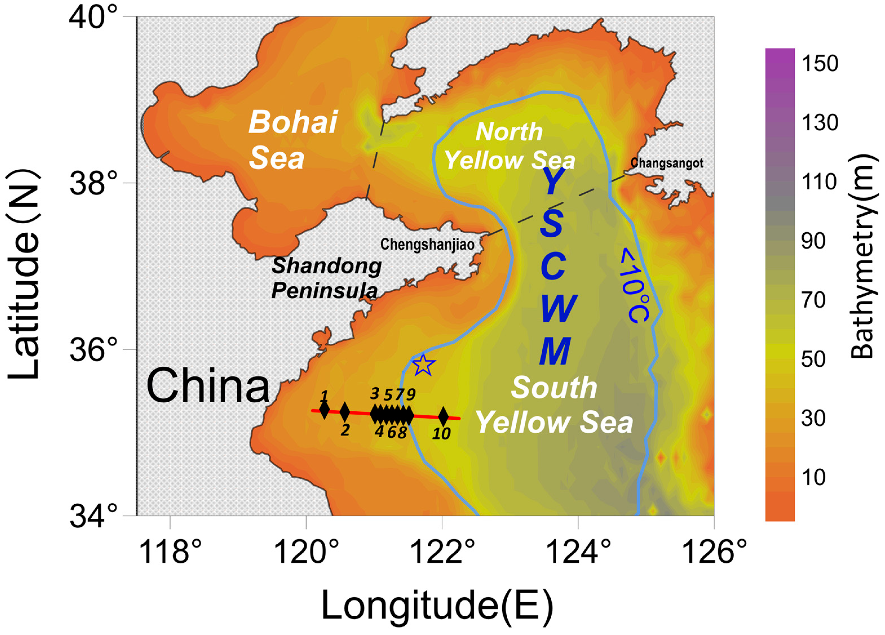
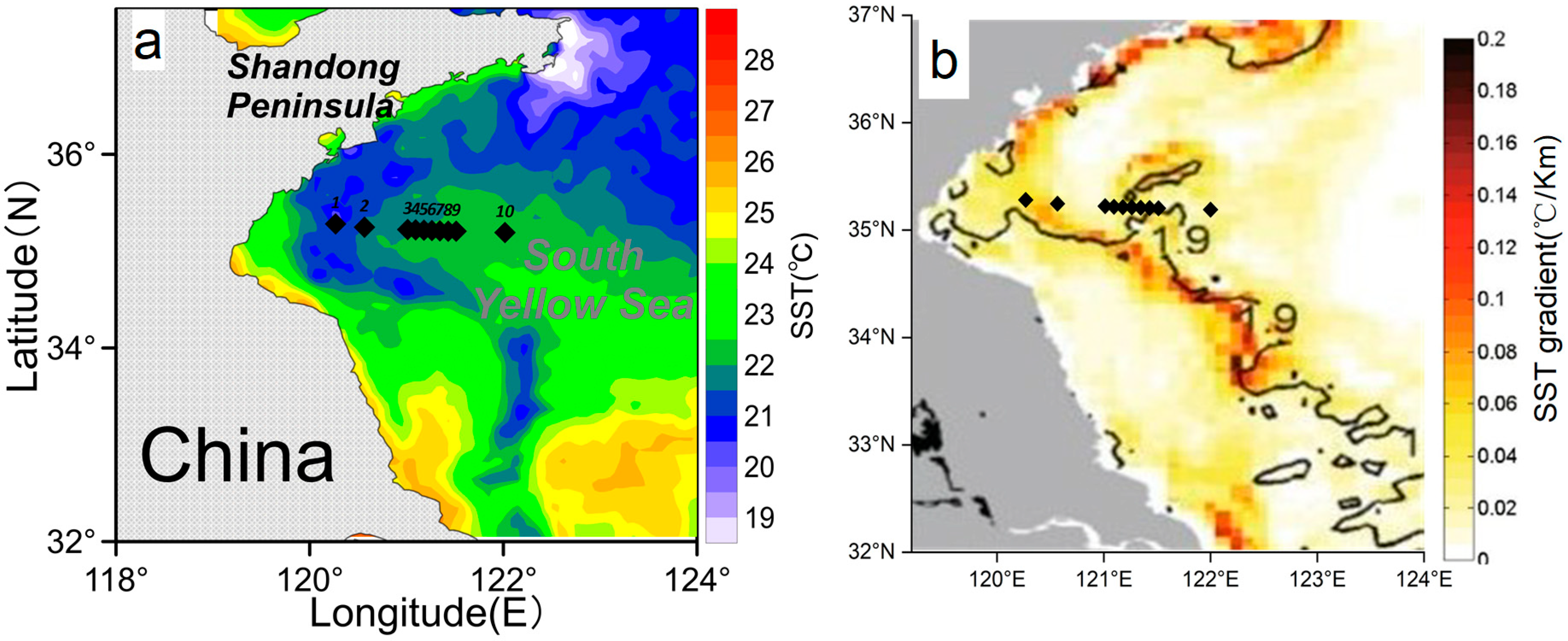
2.1. Survey Information

This study was conducted at the western boundary of the YSCWM in the summers of 2021 and 2022, gathering hydrographic and acoustic data from a fishing boat (LURISHANYU61327, total power: 220 kW) (Table 1). In total, 10 stations were surveyed on this transect (120–122°E), of which stations 3 to 9 were sites of intensive observations near the boundary of the YSCWM, with an interval of about half an hour voyage between two adjacent stations (Table 2, Figure 1). In 2022, we conducted another study at the same profiles and stations, the difference being that this time, a continuous round-trip survey was conducted.

2.2. Date Collection

During each station, hydrological profiles were obtained using a conductivity, temperature, and depth (CTD) instrument (Sea&Sun Technology, CTD-75M type, Trappenkamp, Germany). The acoustic measurements were conducted continuously with a calibrated Simrad EK80 echosounder (KONGSBERG SIMRAD, Kongsberg, Norway) in 2021, operating at a frequency of 120 kHz with a ping rate of 1 transmitted pulse per second. A hull-mounted transducer was placed below the sea surface, and its depth was calibrated with a high scatter value of sea bottom and measured depth. We used a shipboard ADCP (Teledyne RDI 300 kHz) to determine the echo intensity (EI) and velocity profile during the 2022 cruise. The ADCP sampled 1 m vertical bins and 30 s averages.
In addition, the tidal current data were calculated using the Matlab Tide Model Driver toolbox (https://www.esr.org/research/polar-tide-models/tmd-software/, (accessed on 10 March 2022)), which can predict the time series of tidal currents at a given point based on tide components (M2, S2, N2, K2, K1, O1, P1, and M4). Meanwhile, ADCP data in the vicinity of this research area (35.8°N, 122.7°E) in 2013 were used to verify the accuracy of the simulated tidal current data [12] (Figure 2). By comparing with ADCP data, we found that TMD verified the timing of the flood–ebb tide well. It means the TMD data can be utilized in analyzing the influence of the flood–ebb tidal process, even though precise verification of simulated tidal current velocity along the cruise can not be implemented because of the unavailability of the navigable pure tidal current. Furthermore, sea surface temperature (SST) data at a resolution of 0.25° × 0.25° during the survey period were accessed via the Copernicus Marine Environment Monitoring Service (https://marine.copernicus.eu/, (accessed on 15 March 2022)).

2.3. Acoustic Data Analysis

The acoustic data collected from the transects were analyzed with ESP3 V1.4.1., which is an open source software for processing acoustic data and enabling the quantitative, semi-automated analysis of acoustic backscatter [43]. Unnecessary signals (e.g., bubbles at the transducer face, bottom signals, bad pings, and spikes) were first excluded as blank values in the calculations of echo integration. Then, the removal of background noise and estimation of signal-to-noise ratio (SNR) was based on similar classic methods [44]. The maximum background noise level threshold was set to −110 dB according to the prevailing environment. Then, the acoustic data were integrated with a horizontal resolution of 30 s and a vertical resolution of 0.5 m.
The volumetric backscattered intensity (Sv), calculated from the echo integration, is the ratio of the scattered intensity of the acoustic wave in the source direction to the incident wave intensity per unit volume. It is equal to the sum of the backscattered cross-sections of the particles per unit volume [45].
S v = 10   log 10 s v
where sv is the volume scattering coefficient [46]. Therefore, the value of Sv can better reflect the situation of a particle in water, and the scattering characteristics of zooplankton can also be accurately reflected at 120 kHz [47]. According to previous studies, zooplankton are usually aggregated and exhibit a “nepheloid layer” shape in the echogram, while fish are patches or lines [24]. Therefore, based on a more distinct and continuous appearance of the vertically migrated nepheloid layer on the echogram (Figure 3c,d), it can be concluded that zooplankton constitute a major proportion of migrating particles in the water. The study of DVM presented in this paper mainly focuses on zooplankton. Subsequently, the echogram was compared with the hydrographic profile for analysis.
The EI from the ADCP could reflect particle concentrations in the water column; 300 kHz data have been widely used for zooplankton research [48]. Considering that the distance of the ADCP from the surface is 0.5 m and its blind zone below 4.17 m, data deeper than 5 m from the sea surface were excluded. Furthermore, given that EI was only used as an indicator of plankton distribution and not for precise analysis, we qualitatively used these data rather than converting them to backscatter intensity [49]. In this study, the Morse wavelet analysis method was employed on the fluctuations of Sv in the echogram, using the “cwt” function in MATLAB to obtain a time–frequency diagram of fluctuations.
Finally, in order to facilitate the analysis, we used the vertical gradient method to analyze the structure of the thermocline. The thermocline is a layer of water in which oceanic elements change dramatically with depth. When the vertical gradient of a section of the temperature profile is greater than 0.1 °C/m, it is identified as a boundary of the thermocline [50]; the thermocline thickness is the difference in depth between the upper and lower boundaries of the thermocline, and the vertical temperature gradient is the strength of the thermocline (°C/m).
ST = (TUTL)/(DLDU)
where ST is the strength of the thermocline; TU and TL are the temperatures of the upper and lower thermocline boundaries, respectively; and DU and DL are the depths of the upper and lower thermocline boundaries, respectively.
The vertical shear of the horizontal current velocity, velocity shear (VS, s−1), was defined as follows and was used to study its effects on the thermocline:
V S = u z 2 + v z 2
where u and v are the eastward and northward velocity components, respectively, and z is the water depth [51]. Simpson et al. [52] proposed a criterion for predicting the location of tidal fronts based on mechanical energy balance:
S H = l o g   H / U 3
where H is the water depth and U is the amplitude of the tidal velocity. If the position of a given value of the stratification parameter closely coincides with the fronts, the critical value can be used for front detection.

3. Results

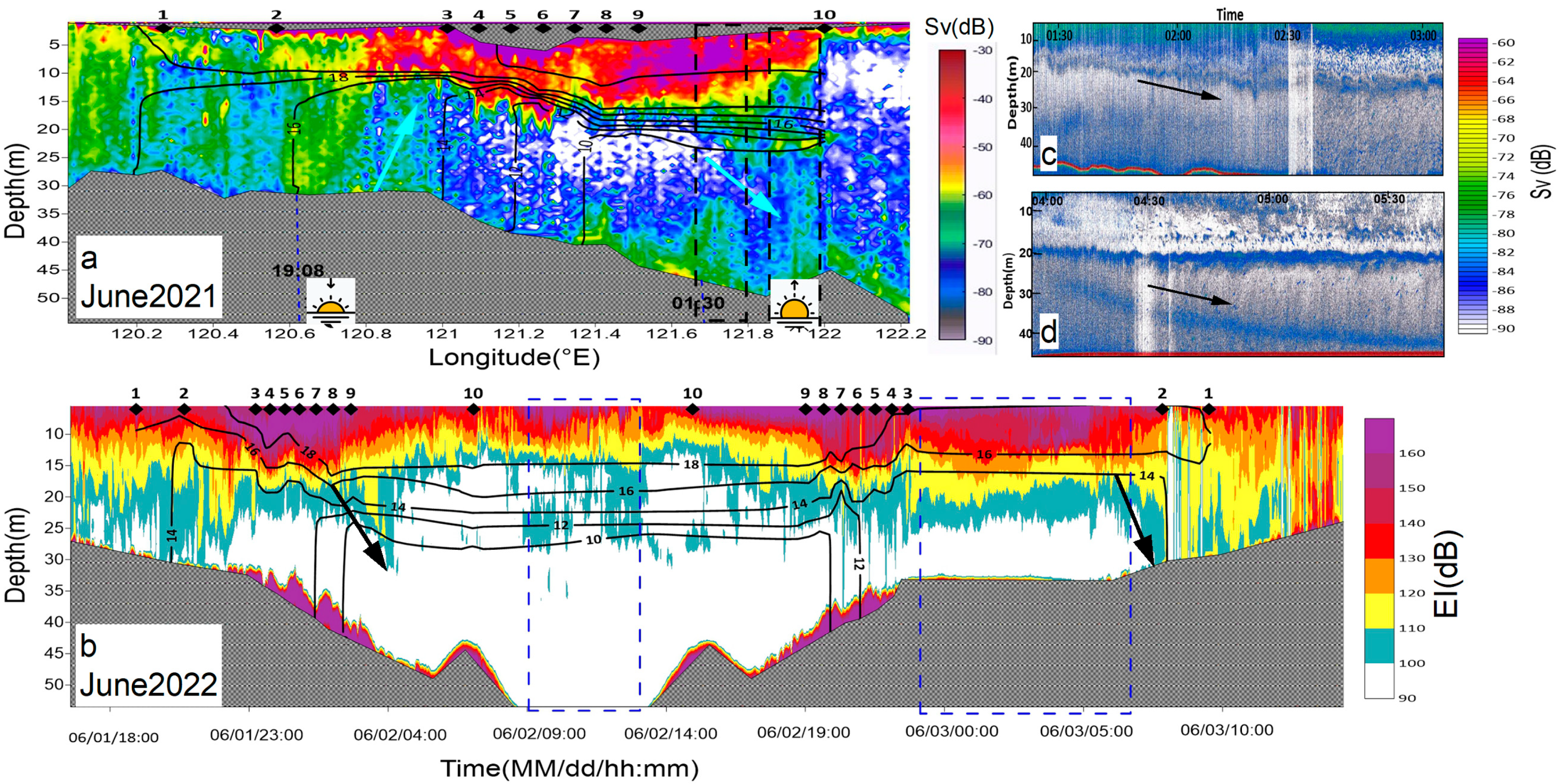
3.1. Overview of Cruises in 2021 and 2022

In general, the CTD observation along the survey section provided an accurate representation of the water column structure in the nearshore and cold water mass areas; particularly, the intensive station observations near the edge of the cold water mass reflected its high-frequency variations. The acoustic data clearly show that, at night, high values of Sv and EI occur in the mixed layer above the thermocline, while during the day, the Sv and EI in the upper layer are clearly weakened and enhanced in the lower layer. This diurnal cyclic variation was evident on both the echosounder EK80 and ADCP, which reflected the DVM of local zooplankton and fish (Figure 3). In addition, it is worth noting that there seems to be a correspondence between the thermocline and Sv or EI. The thermocline at the same point does not seem to be constant throughout the day; these issues are further discussed below.
By comparing the two years’ surveys, the 10 °C isotherm expanded significantly westward and raised upward in 2021. According to the temperature structure, stations 7, 8, 9, and 10 in 2021 and 8, 9, and 10 in 2022, with bottom temperatures lower than 10 °C, are located within the YSCWM. Stations 3 to 7 can be regarded as the boundary of the YSCWM. We repeatedly verified the reliability of acoustic indicators to reflect environmental changes in water under two years of different hydrological conditions. The accurate identification of the YSCWM boundary by the intensive stations laid the foundation for the subsequent comparison of acoustic data with the structure of the water column.

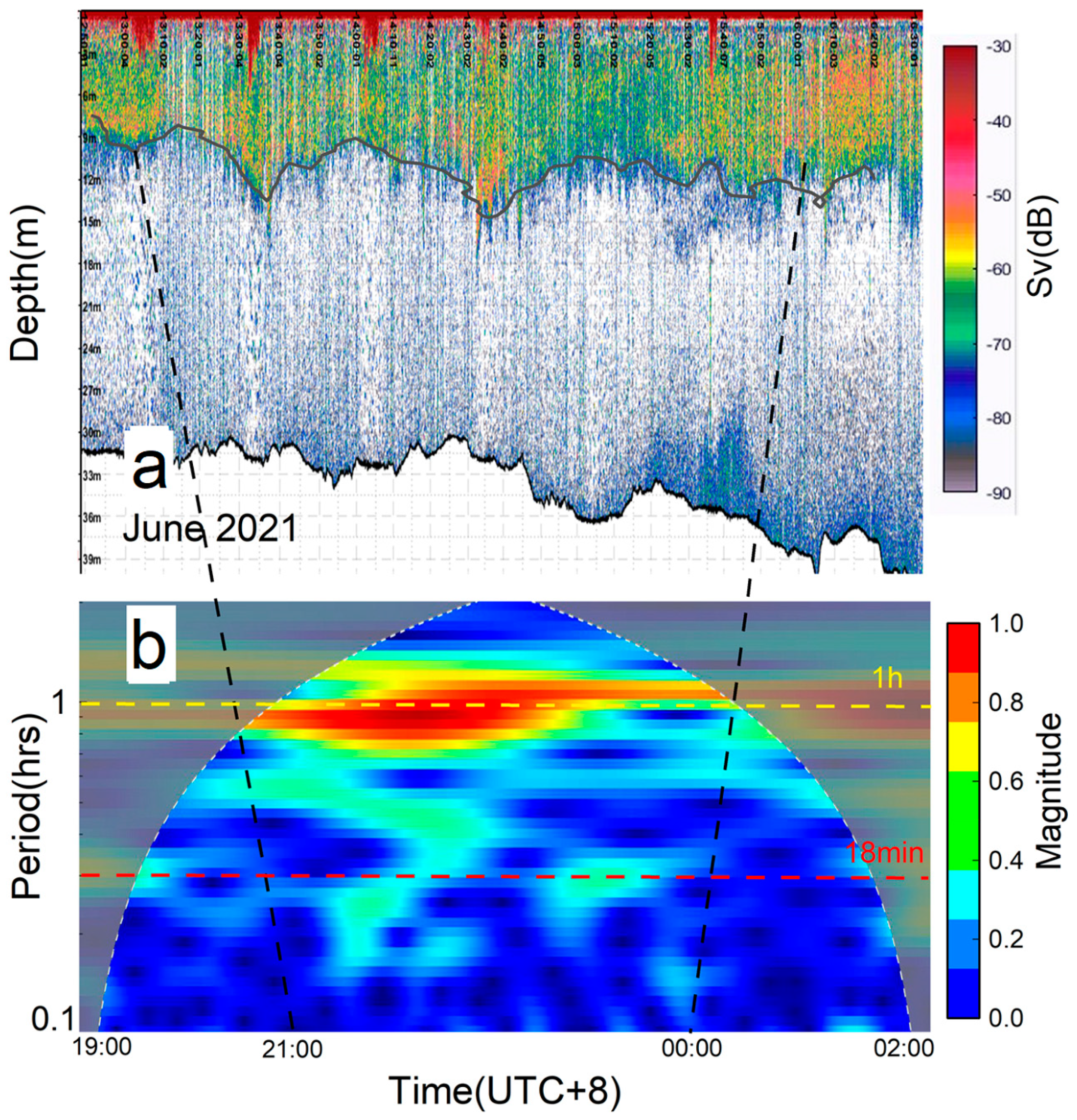
3.2. Characteristics of DVM in Summer in the YS

There was a clear difference in the day-time and night-time distribution of zooplankton, which migrated to the upper mixed layer at night and descended to the bottom during the day. During the survey performed in 2021, according to the echosounder, the upward migration began at 7:08 p.m., 11 min ahead of sunset, and migrated to approximately 12 m depth at 8:00 p.m. The average speed during this period was 0.62 cm/s. The next day, at 1:30 a.m., the zooplankton began their first descent from 16 m to near 24 m. In total, 50 min had elapsed, with an average velocity of 0.27 cm/s (Figure 3c). After staying for some time, at 3:40 a.m., the zooplankton began a second descent to the bottom at a speed of 0.30 cm/s (Figure 3d). The whole migration process was completed before sunrise at 4:42 a.m. A similar phenomenon was reflected in the EI of the ADCP from the 2022 cruise. The two round trips from stations 3 to 9 were conducted at night when the high EI appeared in the surface 15 m layer. At sunrise, between stations 9 and 10 and between stations 2 and 3, we observed two clear migrations downwards. Additionally, in the day-time, near station 10, there was a high EI apparent around 25 m. There is obvious DVM behavior in the Yellow Sea in summer, and there is a potential correlation between the layer to which zooplankton migrate and the structure of the water column; therefore, it would be worthwhile studying the hydrological structure in summer using acoustic remote sensing.

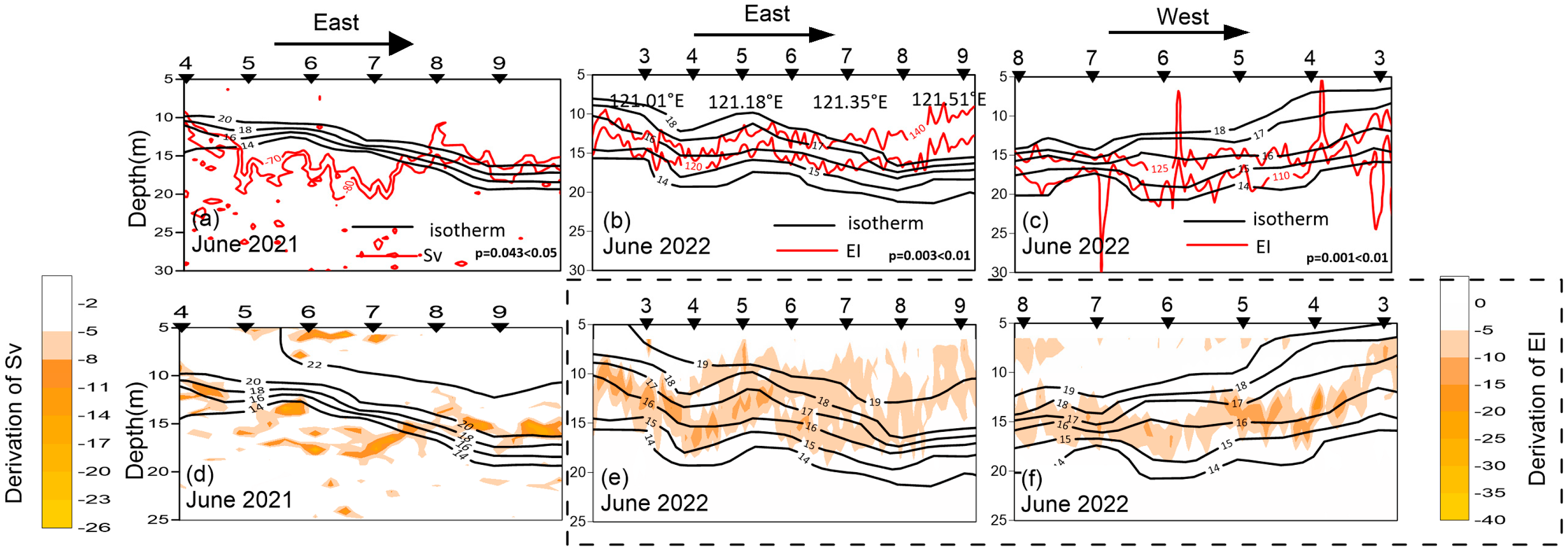
3.3. Hydrological Structure of the YS Based on Acoustic Remote Sensing

By comparing the acoustic data around each CTD cast from the 2021 cruise with the temperature profiles, it was found that the vertical Sv profile responded well to the thermal structure. We selected four representative stations for analysis (Figure 4). At station 1, the nearshore water depth was 27 m. The thermocline was weak, and the zooplankton had not yet migrated to the upper layer, which was mainly distributed from depths of 3 to 21 m. The vertical distribution variation was similar to the chlorophyll-a (chl-a) distribution (Figure 4a). A similar phenomenon occurred in the chl-a maximum layer (CML) at station 10, with zooplankton aggregations near 22 m, which will be further discussed below. Stations 5 and 9 both recorded well into the night, and zooplankton had migrated above 13 and 18 m, respectively (Figure 4b,c). It is clear that the profile lines of Sv and temperature correspond well to each other. Station 10 was observed in the day-time of the next day when the zooplankton had already completed their downward migration (Figure 4d). There was a clear difference compared with the evening echogram, where the high value of Sv appeared in the base of the thermocline or the CML rather than the upper layer. Therefore, unlike at night, when the profile shapes of Sv and temperature were similar, the high Sv during the day also accurately reflected the bottom of the thermocline (Figure 4d).
In addition, we compared the acoustic data and temperature profiles of the whole section in 2021 and 2022 and identified a strong correspondence (Figure 5). We removed some scattered individual echo values (red dots in Figure 5a) to calculate the depth of the echo contour that best matched the isotherm. By selecting three segments of continuous stations that were not affected by zooplankton DVM at night, significant correlations were found between the isotherm, the EI contours, and the Sv contours. In particular, a highly significant correlation was found in the 2022 cruise (p < 0.01). Furthermore, through the first-order derivation of EI and Sv, it was found that the layer with the largest gradient change and the thermocline was also correlated.
In summary, the high-resolution echosounder provided an accurate reflection of not only the vertical distribution numbers and migration behavior of zooplankton but also the internal hydrological structure of the water column. Therefore, based on the verification that the acoustic data can reflect the hydrographic structure, the advantages of high-resolution and spatially continuous observations of acoustic data can be utilized to deeply analyze the effects of fine-scale oceanic processes at the YSCWM boundary on the structure of the water column.

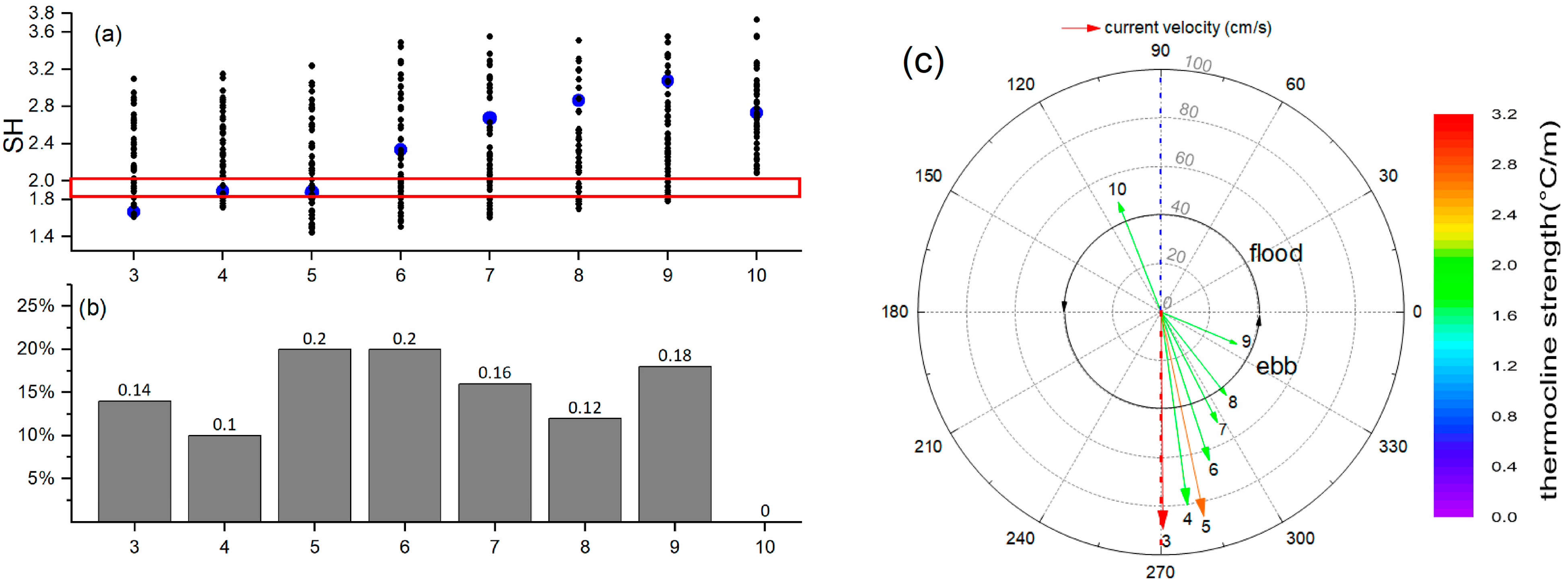
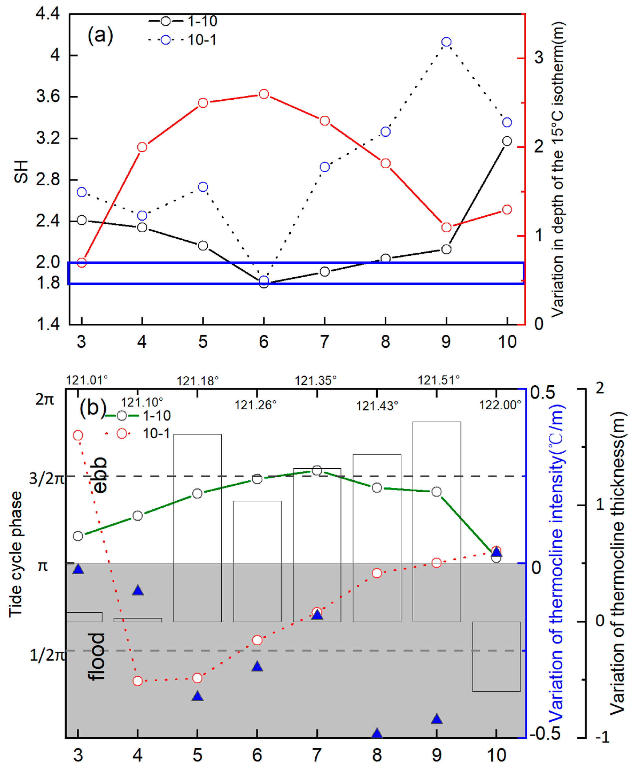
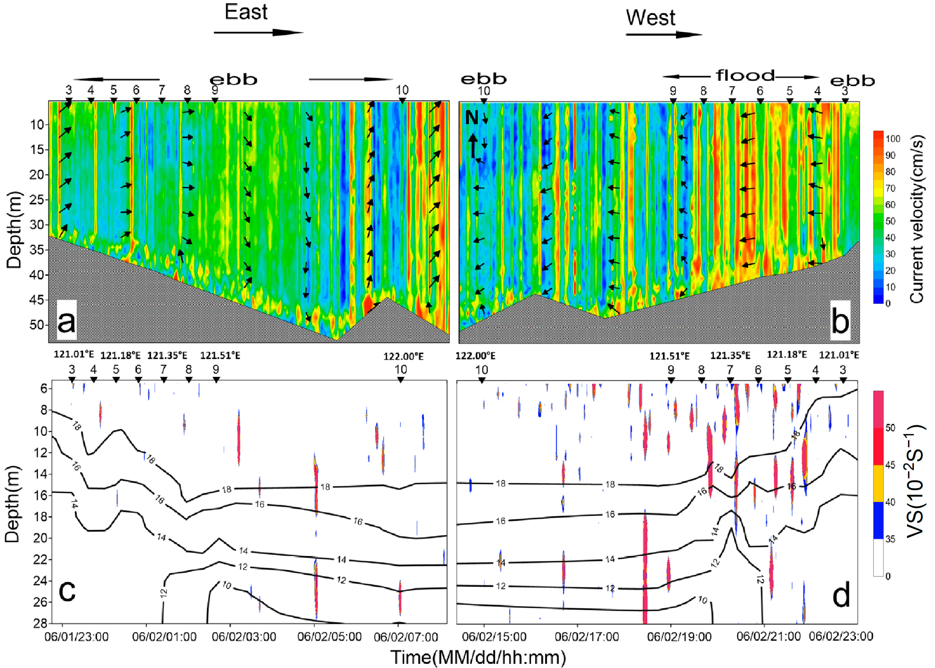
3.4. Fine-Scale Variation in the YSCWM Water Structure

According to the two years’ observations, the following phenomena in the YSCWM were identified: firstly, there were significant fluctuations in the thermocline near the boundary of the YSCWM; secondly, differences in the thermocline and the YSCWM boundary were even found in short-time round-trip comparisons. Stations 1 and 2 are mixed uniform nearshore areas with no apparent stratified structure outside the YSCWM boundary; therefore, they are excluded from the subsequent discussions. We speculate that a number of oceanic processes may be the potential causes, such as internal waves, flood–ebb tidal currents, and upwelling at the water mass boundary.
The comparison of ADCP revealed that the current velocity at stations 3 to 9 on the return journey was significantly larger than that on the outward journey. A larger VS was found near the thermocline at station 10 on the eastward journey and at stations 5 to 9 on the westward journey (Figure 6). On the 2021 cruise, the internal wave was also visible through acoustics; wavelet analysis indicated mainly high-frequency fluctuations with periods of 18 min to 1 h (Figure 7).
We exported the tides for 25 h before and after each station by TMD and analyzed the tidal phase at the time of placing the CTD cast at each station, then performed comparisons with the changes in the thermocline (Figure 8c). Stations 3 and 5 had the strongest effects, reaching 3 °C/m and 2.5 °C/m, respectively; the rest of the stations recorded results between 1 °C/m and 2 °C/m (Figure 8c). We took the short axis of the tidal ellipse as the starting point; 0 to π meant a flood tide; π to 2π was an ebb tide; and stations 3 to 9 were during the ebb tide. However, because stations 3 to 9 recorded very close to each other, within a time interval of about half an hour, and did not differ much from each other in terms of tidal phase, we did not consider it appropriate to use the tidal current to explain the differences in the thermocline between stations. For the 2022 cruise, we compared differences in the tidal phase and thermocline when passing the same station twice in one day. It was clear that on the journey eastward, the tide was mainly ebb, and on the journey westward, the tide was mainly flood; the difference was especially noticeable in stations 4 to 9 (Figure 9b). We used three indicators to measure the variation in the thermocline: (1) the variation in the depth of the 15 °C isotherm; (2) the variation in the intensity and thickness of the thermocline (back minus forth, i.e., positive sign for stronger and thicker thermocline). In order to better explore the effects of different physical ocean processes on the thermocline, we divided the influence of each oceanic process into four conditions by controlling the variables. (1) There was an effect of tide but no shear influence (flood tide in return), as demonstrated at station 4. The depth of the 15 °C isotherm changed by 2 m, and the thermocline exhibited slight weakening (−0.2 °C/m) and thickening (0.1 m). (2) There was an effect of shear but no tide influence. Similar tidal phases with shear occurred on the journey outward but not on the return, as demonstrated at station 10. The depth of the 15 °C isotherm changed by 1.3 m, and the thermocline exhibited slight strengthening (0.03 °C/m) and thinning (−0.6 m). (3) Dual effects of tide and shear. Different tidal phases with shear effects were observed on the return journey, as demonstrated at stations 5 to 9. There were 2 to 3 m changes in the 15 °C isotherms at stations 5, 6, and 7, and a significant weakening of the thermocline, especially at stations 8 and 9, where it was close to 0.5 °C/m. The thermocline was also significantly thicker than 1 m. (4) No tide or shear effects. With similar tidal phases and no shear effects, as demonstrated at station 3, the three thermocline indicators did not change significantly.
In addition, numerical models suggest that upwelling plays an important role in the variation in the YSCWM western boundary [1]. Following Zhao [53], we used 1.8–2.0 as a threshold to determine the position of fronts caused by tidal upwelling. The values observed for stations 4 and 5 were within this threshold, and analysis of one tidal cycle 25 h before and after the deployment of the CTD at each station showed that between 10% and 20% of the time, the results recorded at stations 3 to 9 satisfied this range (Figure 8a,b). Stations 5 and 6 had the highest chance of being within this threshold, as well as exhibiting the largest changes in isotherms at these two stations in 2022 (Figure 9a). This indicated the presence of recurrent upwelling in the western boundary region of the YSCWM, which can affect the strength of the thermocline.
In general, both the flood tide and current shear can cause the thermocline to weaken and thicken and the isotherm to change by 1 to 3 m; these short-term changes are made more pronounced when both are present. Near the boundary of the YSCWM, upwelling can also cause changes in the thermocline and isotherms.

4. Discussion

4.1. The DVM of Zooplankton in Summer in the YS

The DVM of zooplankton is a very common cyclical variation in marine ecosystems and has been reported both on the continental shelf and in the deep sea. DVM is performed for a number of reasons, an important one being for better foraging opportunities and the avoidance of predation from visual predators [54,55]. DVM is predominantly regulated by light; thus, zooplankton stays shallower at night than during the day [56]. Our findings agreed with those in previous studies. Although we did not perform continuous observations at the same stations, fortunately, the water depth did not change much during the DVM in the study, and the duration was not long. Therefore, we assumed that other nearby DVMs were conducted almost simultaneously. The fixed-point long-term observations performed using ADCP in summer in the SYS showed that zooplankton migrated upward at a speed of 0.12 to 0.55 cm/s, starting around 6 p.m., and migrated to the bottom at a speed of 0.1 to 0.6 cm/s, starting at 5 a.m. [57]. In the central YS at a water depth of about 75 m, Kim et al. [24] identified a nepheloid layer DVM consisting of copepods and Euphausia pacifica with velocities of about 0.5 cm/s using acoustic and net sampling. This was similar to the migration speed we observed but less than the global average DVM speed, probably because of the shallower depths; diel vertical migration is generally performed more quickly at deeper water depths [58].
Compared with traditional net tows and trawls, acoustic data can provide a higher temporal resolution remote sensing perspective to study the long-term or short-term spatial and temporal variability in DVM [19,23,28]. Although we did not conduct zooplankton sampling concurrently with acoustic observations, zooplankton data obtained during the summer of 2019 in the vicinity of this study area can provide some reference [59]. WP-2 net results (conical type; mouth area, 0.25 m2; mesh size, 200 µm) showed that the dominant species were Paracalanus parvus and Oithona similis. According to previous studies, Paracalanus parvus ascended to about 10 m at night and descended near the thermocline after sunrise, while Oithona similis rose from below the thermocline to the upper thermocline after sunset [60]. This suggests that the thermocline in the YS in summer is an important factor influencing zooplankton distribution [3], which is consistent with our acoustic response to the presence of high EI near the thermocline during day-time.
Therefore, acoustic remote sensing demonstrated that the DVM behavior of zooplankton is closely related to the stratified structure of the water column. This was shown in the echograms: the Sv and temperature profiles were very similar at night, and the high Sv reflected the base of the thermocline during the day after the zooplankton migrated downward.

4.2. The Potential Utilization of Acoustic Remote Sensing on Reflecting High-Resolution Ocean Structures

Through comparison, we found that there is a good correspondence between the Sv and the thermocline for performing both stationary and cruising observations. In fact, a common method is to determine the mixed-layer depth (MLD), thermocline depth, or pycnocline depth through a large Sv gradient [31,33]. Stranne et al. [31] mapped the MLD in the Arctic Ocean using ship-mounted echo sounders, reporting a success rate of 95% in the open ocean and 75% in the nearshore, with the lower success rate mainly due to the greater abundance of biological scatters and shallower water depths; however, the large draft of the ship (7 m) resulted in fewer valid data. Thus, smaller boats with a smaller draft are more suitable for tracking MLD offshore. In the SYS, although the general correspondence was good, there was still a biological influence on the echoes, e.g., the presence of a subsurface chl-a maximum layer (SCML) in the lower part of the thermocline at station 10, which led to a concentration of zooplankton in this area and a high Sv in the echogram (Figure 4d). Numerous previous studies have shown that the trend in nutrient distribution is consistent with the deep distribution pattern of the SCML due to the stratification of seawater in summer [61]. This is because the depth of the SCML corresponds well to the bottom of the thermocline, making the day-time high Sv a good indication of the lower boundary of the thermocline. The thermocline in the SYS is also usually located in the euphotic zone and has good photosynthetic conditions, where phytoplankton mainly absorb nutrients to form the SCML [62], whereas copepods, such as Calanus sinicus, migrate to the SCML in search of abundant food to achieve optimal growth conditions [63]. In addition, the frequency of the echosounder itself and the strength of the thermocline can affect the accuracy of the acoustic method. The experimental method confirmed that in shallow waters of the YS in summer, a thermocline greater than 1.3 °C/m can be detected at a frequency of 200 kHz [64].
Water column stratification is a very common phenomenon in the ocean, and it represents a natural barrier. It is closely associated with the vertical habitat distribution of zooplankton and fish. Thus, acoustic remote sensing is a good bridge linking the distribution of biology to the water column structure. For example, in the highly productive eastern South Pacific, off Peru, which is home to the world’s largest single species of the Peruvian anchovy (Engraulis ringens), the depth of the oxycline matched to the pycnocline was successfully monitored using an echosounder [33].
Many contemporary fishing vessels are equipped with acoustic devices, and they frequently navigate various seas. This characterizes a new approach to understanding the structure of the water column on a global scale. Although acoustic remote sensing cannot fully replace in situ surveys such as CTD, it does represent a novel way of capturing the structure of a water column over a larger coverage area and at a higher temporal resolution, acting as a bridge to efficiently connect discrete CTD stations. In the future, this method could be used more widely for global water stratification data collection and could be an important complement to ARGO float profiles [30] and large-area satellite remote sensing surface temperature and salinity data [65], as well as providing supporting data for future model estimates of the thermocline or MLD [66].

4.3. Mechanisms of the Influence of Key Ocean Processes on the YSCWM Structure

Firstly, the effect of the tide on the structure of the water column was assessed. Based on a Hybrid Coordinate Ocean Model (HYCOM), Ren et al. [16] demonstrated that upwelling and tidal mixing were the main causes of Subei bank front formation in the YS during summer. The location of the front, as determined by the SH index and calculated by the model, is consistent with the results of the present study (Figure 10b). A more intuitive manifestation of this is the tidal mixing of cold water from deeper layers to the upper layers, resulting in a decrease in SST and, thus, the surface cold patches (SCPs) observable on satellite remote sensing maps (Figure 10a). This has also been confirmed by historical observations [67]. In essence, the upwelling of the YS is caused by strong tidal mixing over the sloping topography. It occurs in a narrow transition zone between well-mixed shallow water and stratified deep water, the tidal mixing front (TMF), where large differences in temperature (or density) at the front surface lead to considerable oblique baroclinic pressure gradient force (PGF) along the bottom. The upwelling carries the cold water from the bottom upwards, with corresponding downwelling in the upper layers, thus affecting the vertical stratification of the water column structure [1].
Another concern is flood–ebb asymmetry on the continental shelf: mixing is stronger and stratification is weaker at flood tides, with the opposite at ebb tides [68]. In the present study, this asymmetry resulted in a variation of 0.2 to 0.5 °C/m in the intensity of the thermocline (Figure 9b). The mechanism behind this phenomenon may be the tidal straining effect [69]. Due to the bottom friction effect, the current velocity in the upper layer was high, while that in the bottom layer was low, forming a vertical shear of the current velocity. Before the start of the ebb tide, the vertical mixing was uniform, while at the start of the ebb tide, due to the vertical shear effect, the current velocity in the upper layer was greater than that in the bottom layer. The slower-flowing, high-density water in the bottom layer was occupied by the lower-density water in the upper layer, forming a stronger stratification, i.e., during the ebb tide, it becomes more stratified. In addition, this asymmetry in bed stress may be responsible for the weaker stratification on the flood tide [70]. As to which mechanism is dominant in the SYS, further research is needed.
Lastly, the intense current shear that occurred in the thermocline cannot be ignored. The internal waves continually triggered strong velocity shear on the thermocline as they propagated, thus providing the impetus for mixing above and below [37]. The strengthening of thermocline mixing is the result of shear instability within the thermocline [71], and we also found that strong shear in the upper thermocline weakens the thermocline. In addition to the observation of internal waves by acoustics on our 2021 cruise, not coincidentally, in situ observations and satellite images revealed the presence of frequent internal solitary waves (ISWs) in the YS [72]. Liu et al. [10] carried out 25 h observations using upward-looking 600 kHz ADCP and an MSS-60 microstructure profiler at the overlap of station 9 (35°N, 121.5°E) established in our study and found that propagation of the ISW produced a large vertical velocity shear, resulting in an average vertical displacement of 4 m in the pycnocline, with period peaks again of around 11 to 43 min. Therefore, the fluctuations observed in this study are likely to be ISWs.
Using high-frequency acoustic remote sensing technology can enable very high-resolution measurements in a larger range because the typical ping rate is higher compared with direct microstructure instruments that perform analyses every few minutes. During the passage of nonlinear internal waves, some oceanic microstructures, such as Kelvin–Helmholtz shear instability, can be better observed by acoustics [73].

4.4. YS Boundary Area Hydrodynamic–Hydrologic–Ecological Variation Pattern

From the above analysis, we found that acoustic remote sensing accurately reflects the hydrodynamic–hydrological–ecological variables in the water because it captured scatters from biotic and abiotic sources in the received reflected sound signals. The variation pattern is summarized in Figure 11.
In summer in the YSCWM, weakening and thickening of the stratified structure, as well as vertical displacement of the isotherms by several meters on short time scales, is facilitated by the excitation of strong shear during IW propagation, which promotes mixing of the water column. A similar situation occurs in flood tides, while the ebb tides exert a contrasting influence. This change becomes more obvious when flood tide and shear occur simultaneously. Additionally, in the area of tidal fronts near the YSCWM boundary, upwelling induced by tidal mixing can also cause significant fluctuations in isotherms.
Although the YSCWM only constitutes a small part of the YS, its hypoxia, acidification, and high nutrient content make it vital in the YS ecosystem [74]. Zhai [75] predicted that by 2050, acidifying seawater will cover 50% of the YS seafloor, which will severely impact the local ecosystem. How this will lead to changes in the habitat of cold-water fish and the DVM of zooplankton in the YSCWM needs to be studied in the longer term.

5. Conclusions

To study the influence of fine-scale ocean processes on water structure at the YSCWM boundary, high-resolution acoustic remote sensing and intensive CTD station site placements were carried out in 2021 and 2022.
(1)
We observed significant high-frequency thermocline fluctuations at the YSCWM boundary; zooplankton were below the thermocline during the day and migrated above it at night;
(2)
Through the ground-truthing of CTD, the YS summer thermocline can be successfully detected using acoustic remote sensing;
(3)
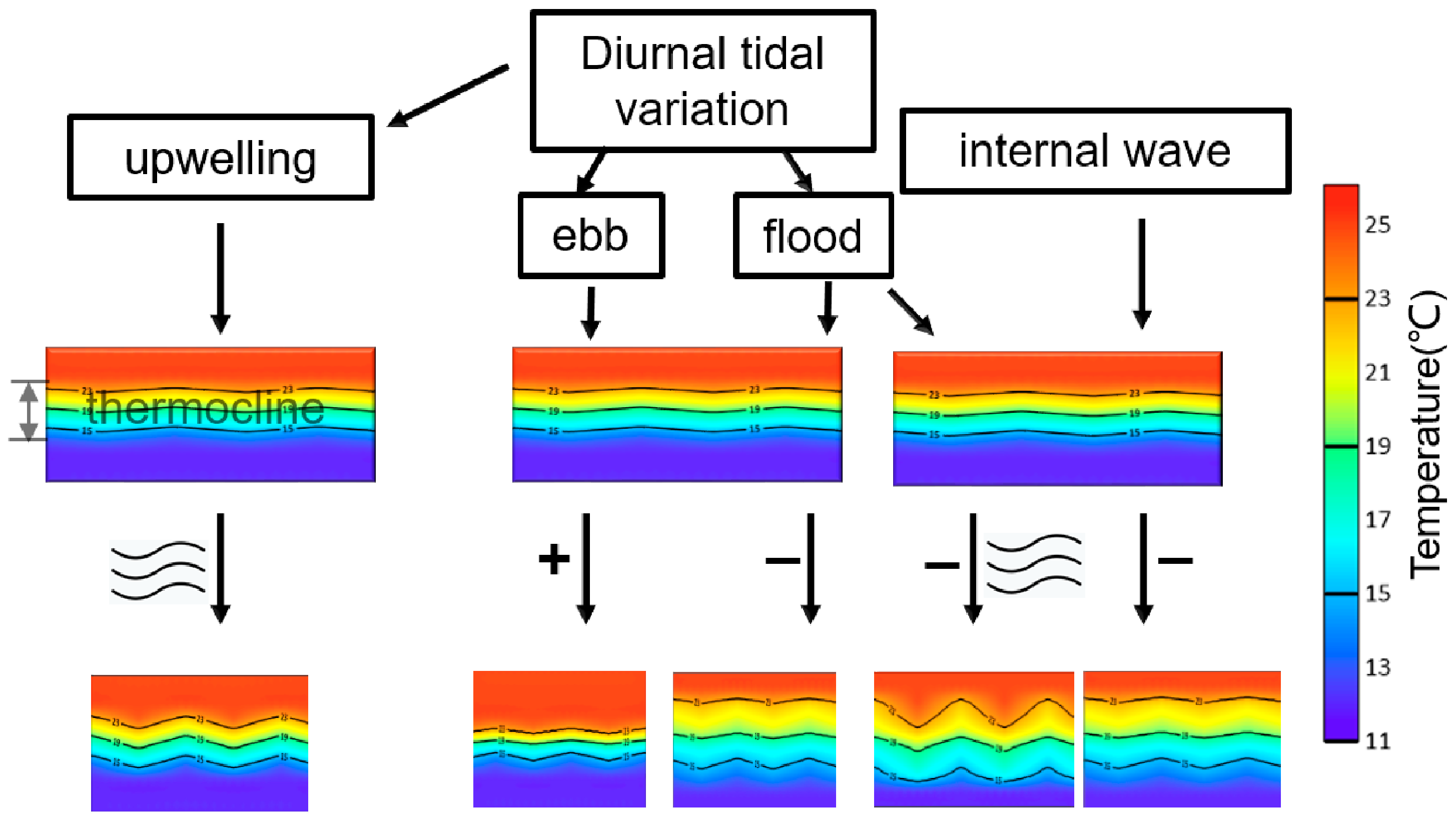
Shear caused by internal waves and flood tides negatively weaken the stratification of the water column, which is more pronounced when the two mechanisms are concurrent (weakening of the thermocline by 0.5 °C/m); ebb tides have a positive effect on water column stratification. In the area of tidal fronts, tide-induced upwelling can also cause significant fluctuations in isotherms.
This study demonstrates a promising new way of studying the fine-scale hydrodynamic–hydrologic–ecological aspects of key regions through acoustic remote sensing. It is an efficient technique for covering a larger area compared with traditional methods and makes it possible to study fine-scale changes in the structure of the water column with the advantage of higher-resolution data. A study on the effects of regional complex hydrodynamic processes on the structure of the water column will contribute to a better understanding of changes in the ecosystem.

Author Contributions

Conceptualization, Y.L.; Data curation, H.W., W.Z., P.S. and S.M.; Formal analysis, L.N.; Funding acquisition, J.L., Y.T. and Q.G.; Investigation, H.W., W.Z. and S.M.; Project administration, Y.T.; Resources, J.L., Z.Y. and Q.G.; Supervision, J.L. and Y.T.; Visualization, Y.L.; Writing—original draft, L.N.; Writing—review and editing, J.L., Y.T., P.S. and Z.Y. All authors have read and agreed to the published version of the manuscript.

Funding

This study was supported by the National Key Research and Development Program of China (Project No. 2019YFD0901000) and the National Natural Science Foundation of China, Grant/Award Number: 41930534, 41806190. The Fundamental Research Funds for the Central Universities (202264003, 202362002).

Data Availability Statement

Data are contained within the article. The processed survey data used to construct the figures presented in this paper are available upon reasonable request from the corresponding author ([email protected]).

Acknowledgments

We thank the crew for their help with the cruise investigation.

Conflicts of Interest

The authors declare no conflict of interest.

References

  1. Lue, X.; Qiao, F.; Xia, C.; Wang, G.; Yuan, Y. Upwelling and surface cold patches in the Yellow Sea in summer: Effects of tidal mixing on the vertical circulation. Cont. Shelf Res. 2010, 30, 620–632. [Google Scholar] [CrossRef]
  2. Oh, K.-H.; Lee, S.; Song, K.-M.; Lie, H.-J.; Kim, Y.-T. The temporal and spatial variability of the Yellow Sea Cold Water Mass in the southeastern Yellow Sea, 2009-2011. Acta Oceanol. Sin. 2013, 32, 1–10. [Google Scholar] [CrossRef]
  3. Ge, R.; Chen, H.; Liu, G.; Zhu, Y.; Jiang, Q. Diel vertical migration of mesozooplankton in the northern Yellow Sea. J. Oceanol. Limnol. 2021, 39, 1373–1386. [Google Scholar] [CrossRef]
  4. Li, M.; Zhong, L. Flood-ebb and spring-neap variations of mixing, stratification and circulation in Chesapeake Bay. Cont. Shelf Res. 2009, 29, 4–14. [Google Scholar] [CrossRef]
  5. Chu, P.C.; Fralick, C.R.; Haeger, S.D.; Carron, M.J. A parametric model for the Yellow Sea thermal variability. J. Geophys. Res. Ocean. 1997, 102, 10499–10507. [Google Scholar] [CrossRef]
  6. Qiao, F.; Ma, J.; Xia, C.; Yang, Y.; Yuan, Y. Influences of the surface wave-induced mixing and tidal mixing on the vertical temperature structure of the Yellow and East China Seas in summer. Prog. Nat. Sci. 2006, 16, 739–746. [Google Scholar] [CrossRef]
  7. Park, S.; Chu, P.C. Synoptic distributions of thermal surface mixed layer and thermocline in the southern Yellow and East China Seas. J. Oceanogr. 2007, 63, 1021–1028. [Google Scholar] [CrossRef]
  8. Li, J.; Jiang, F.; Wu, R.; Zhang, C.; Tian, Y.; Sun, P.; Yu, H.; Liu, Y.; Ye, Z.; Ma, S.; et al. Tidally Induced Temporal Variations in Growth of Young-of-the-Year Pacific Cod in the Yellow Sea. J. Geophys. Res. Ocean. 2021, 126, 6696. [Google Scholar] [CrossRef]
  9. Liu, K.; Sun, J.; Guo, C.; Yang, Y.; Yu, W.; Wei, Z. Seasonal and Spatial Variations of the M-2 Internal Tide in the Yellow Sea. J. Geophys. Res. Ocean. 2019, 124, 1115–1138. [Google Scholar] [CrossRef]
  10. Liu, Z.; Wei, H.; Lozovatsky, I.D.; Fernando, H.J.S. Late summer stratification, internal waves, and turbulence in the Yellow Sea. J. Mar. Syst. 2009, 77, 459–472. [Google Scholar] [CrossRef]
  11. Xu, P.; Yang, W.; Zhu, B.; Wei, H.; Zhao, L.; Nie, H. Turbulent mixing and vertical nitrate flux induced by the semidiurnal internal tides in the southern Yellow Sea. Cont. Shelf Res. 2020, 208, 104240. [Google Scholar] [CrossRef]
  12. Li, J.; Li, G.; Xu, J.; Dong, P.; Qiao, L.; Liu, S.; Sun, P.; Fan, Z. Seasonal evolution of the Yellow Sea Cold Water Mass and its interactions with ambient hydrodynamic system. J. Geophys. Res. Ocean. 2016, 121, 6779–6792. [Google Scholar] [CrossRef]
  13. Huang, M.; Liang, X.S.; Wu, H.; Wang, Y. Different Generating Mechanisms for the Summer Surface Cold Patches in the Yellow Sea. Atmos. Ocean. 2018, 56, 199–211. [Google Scholar] [CrossRef]
  14. Wang, B.; Wu, L.; Zhao, N.; Liu, T.; Hirose, N. Summer Wind Effects on Coastal Upwelling in the Southwestern Yellow Sea. J. Mar. Sci. Eng. 2021, 9, 1021. [Google Scholar] [CrossRef]
  15. Meng, Q.; Li, P.; Zhai, F.; Gu, Y. The vertical mixing induced by winds and tides over the Yellow Sea in summer: A numerical study in 2012. Ocean. Dyn. 2020, 70, 847–861. [Google Scholar] [CrossRef]
  16. Ren, S.; Xie, J.; Zhu, J. The Roles of Different Mechanisms Related to the Tide-induced Fronts in the Yellow Sea in Summer. Adv. Atmos. Sci. 2014, 31, 1079–1089. [Google Scholar] [CrossRef]
  17. Holliday, D.V.; Pieper, R.E. Bioacoustical Oceanography At High-Frequencies. Ices J. Mar. Sci. 1995, 52, 279–296. [Google Scholar] [CrossRef]
  18. Cisewski, B.; Strass, V.H.; Rhein, M.; Kraegefsky, S. Seasonal variation of diel vertical migration of zooplankton from ADCP backscatter time series data in the Lazarev Sea, Antarctica. Deep. Sea Res. Part I-Oceanogr. Res. Pap. 2010, 57, 78–94. [Google Scholar] [CrossRef]
  19. Diaz-Astudillo, M.; Caceres, M.A.; Landaeta, M.F. Zooplankton structure and vertical migration: Using acoustics and biomass to compare stratified and mixed fjord systems. Cont. Shelf Res. 2017, 148, 208–218. [Google Scholar] [CrossRef]
  20. Brierley, A.S.; Brandon, M.A.; Watkins, J.L. An assessment of the utility of an acoustic Doppler current profiler for biomass estimation. Deep. Sea Res. Part I-Oceanogr. Res. Pap. 1998, 45, 1555–1573. [Google Scholar] [CrossRef]
  21. Valle-Levinson, A.; Castro, L.; Caceres, M.; Pizarro, O. Twilight vertical migrations of zooplankton in a Chilean fjord. Prog. Oceanogr. 2014, 129, 114–124. [Google Scholar] [CrossRef]
  22. Escobar-Flores, P.C.; Ladroit, Y.; O’Driscoll, R.L. Acoustic Assessment of the Micronekton Community on the Chatham Rise, New Zealand, Using a Semi-Automated Approach. Front. Mar. Sci. 2019, 6, 507. [Google Scholar] [CrossRef]
  23. Perelman, J.N.; Ladroit, Y.; Escobar-Flores, P.; Firing, E.; Drazen, J.C. Eddies and fronts influence pelagic communities across the eastern Pacific ocean. Prog. Oceanogr. 2023, 211, 102967. [Google Scholar] [CrossRef]
  24. Kim, H.; Kim, G.; Kim, M.; Kang, D. Spatial Distribution of Sound Scattering Layer and Density Estimation of Euphausia pacifica in the Center of the Yellow Sea Bottom Cold Water Determined by Hydroacoustic Surveying. J. Mar. Sci. Eng. 2022, 10, 10056. [Google Scholar] [CrossRef]
  25. Aparna, S.G.; Desai, D.V.; Shankar, D.; Anil, A.C.; Dora, S.; Khedekar, R. Seasonal cycle of zooplankton standing stock inferred from ADCP backscatter measurements in the eastern Arabian Sea. Prog. Oceanogr. 2022, 203, 102766. [Google Scholar] [CrossRef]
  26. Dwinovantyo, A.; Manik, H.M.; Prartono, T.; Susilohadi, S.; Mukai, T. Variation of Zooplankton Mean Volume Backscattering Strength from Moored and Mobile ADCP Instruments for Diel Vertical Migration Observation. Appl. Sci. 2019, 9, 1851. [Google Scholar] [CrossRef]
  27. Song, Y.; Yang, J.; Wang, C.; Sun, D. Spatial patterns and environmental associations of deep scattering layers in the northwestern subtropical Pacific Ocean. Acta Oceanol. Sin. 2022, 41, 139–152. [Google Scholar] [CrossRef]
  28. Liu, Y.; Guo, J.; Xue, Y.; Sangmanee, C.; Wang, H.; Zhao, C.; Khokiattiwong, S.; Yu, W. Seasonal variation in diel vertical migration of zooplankton and micronekton in the Andaman Sea observed by a moored ADCP. Deep. Sea Res. Part I-Oceanogr. Res. Pap. 2022, 179, 103663. [Google Scholar] [CrossRef]
  29. Lee, H.; Cho, S.; Kim, W.; Kang, D. The diel vertical migration of the sound-scattering layer in the Yellow Sea Bottom Cold Water of the southeastern Yellow sea: Focus on its relationship with a temperature structure. Acta Oceanol. Sin. 2013, 32, 44–49. [Google Scholar] [CrossRef]
  30. Ker, S.; Le Gonidec, Y.; Marie, L. Multifrequency seismic detectability of seasonal thermoclines assessed from ARGO data. J. Geophys. Res. Ocean. 2016, 121, 6035–6060. [Google Scholar] [CrossRef]
  31. Stranne, C.; Mayer, L.; Jakobsson, M.; Weidner, E.; Jerram, K.; Weber, T.C.; Anderson, L.G.; Nilsson, J.; Bjork, G.; Gardfeldt, K. Acoustic mapping of mixed layer depth. Ocean Sci. 2018, 14, 503–514. [Google Scholar] [CrossRef]
  32. Grados, D.; Bertrand, A.; Colas, F.; Echevin, V.; Chaigneau, A.; Gutierrez, D.; Vargas, G.; Fablet, R. Spatial and seasonal patterns of fine-scale to mesoscale upper ocean dynamics in an Eastern Boundary Current System. Prog. Oceanogr. 2016, 142, 105–116. [Google Scholar] [CrossRef]
  33. Bertrand, A.; Ballon, M.; Chaigneau, A. Acoustic Observation of Living Organisms Reveals the Upper Limit of the Oxygen Minimum Zone. PLoS ONE 2010, 5, e1033. [Google Scholar] [CrossRef] [PubMed]
  34. Fer, I.; Nandi, P.; Holbrook, W.S.; Schmitt, R.W.; Paramo, P. Seismic imaging of a thermohaline staircase in the western tropical North Atlantic. Ocean Sci. 2010, 6, 621–631. [Google Scholar] [CrossRef]
  35. Stranne, C.; Mayer, L.; Weber, T.C.; Ruddick, B.R.; Jakobsson, M.; Jerram, K.; Weidner, E.; Nilsson, J.; Gardfeldt, K. Acoustic Mapping of Thermohaline Staircases in the Arctic Ocean. Sci. Rep. 2017, 7, 15192. [Google Scholar] [CrossRef]
  36. Koterayama, W.; Yamaguchi, S.; Yokobiki, T.; Yoon, J.H.; Hase, H. Space-continuous measurements on ocean current and chemical properties with the intelligent towed vehicle “Flying Fish”. IEEE J. Ocean. Eng. 2000, 25, 130–138. [Google Scholar] [CrossRef]
  37. Moum, J.N.; Farmer, D.M.; Smyth, W.D.; Armi, L.; Vagle, S. Structure and generation of turbulence at interfaces strained by internal solitary waves propagating shoreward over the continental shelf. J. Phys. Oceanogr. 2003, 33, 2093–2112. [Google Scholar] [CrossRef]
  38. Lavery, A.C.; Schmitt, R.W.; Stanton, T.K. High-frequency acoustic scattering from turbulent oceanic microstructure: The importance of density fluctuations. J. Acoust. Soc. Am. 2003, 114, 2685–2697. [Google Scholar] [CrossRef]
  39. Feng, Y.; Tang, Q.; Li, J.; Sun, J.; Zhan, W. Internal Solitary Waves Observed on the Continental Shelf in the Northern South China Sea From Acoustic Backscatter Data. Front. Mar. Sci. 2021, 8, 734075. [Google Scholar] [CrossRef]
  40. Bertrand, A.; Grados, D.; Colas, F.; Bertrand, S.; Capet, X.; Chaigneau, A.; Vargas, G.; Mousseigne, A.; Fablet, R. Broad impacts of fine-scale dynamics on seascape structure from zooplankton to seabirds. Nat. Commun. 2014, 5, 6239. [Google Scholar] [CrossRef]
  41. Lennert-Cody, C.E.; Franks, P.J.S. Plankton patchiness in high-frequency internal waves. Mar. Ecol. Prog. Ser. 1999, 186, 59–66. [Google Scholar] [CrossRef]
  42. Embling, C.B.; Sharples, J.; Armstrong, E.; Palmer, M.R.; Scott, B.E. Fish behaviour in response to tidal variability and internal waves over a shelf sea bank. Prog. Oceanogr. 2013, 117, 106–117. [Google Scholar] [CrossRef]
  43. Ladroit, Y.; Escobar-Flores, P.C.; Schimel, A.C.; O’Driscoll, R.L. ESP3: An open-source software for the quantitative processing of hydro-acoustic data. Softwarex 2020, 12, 100581. [Google Scholar] [CrossRef]
  44. De Robertis, A.; Higginbottom, I. A post-processing technique to estimate the signal-to-noise ratio and remove echosounder background noise. Ices J. Mar. Sci. 2007, 64, 1282–1291. [Google Scholar] [CrossRef]
  45. Iida, K.; Mukai, T.; Hwang, D.J. Relationship between acoustic backscattering strength and density of zooplankton in the sound-scattering layer. Ices J. Mar. Sci. 1996, 53, 507–512. [Google Scholar] [CrossRef]
  46. MacLennan, D.N.; Fernandes, P.G.; Dalen, J. A consistent approach to definitions and symbols in fisheries acoustics. Ices J. Mar. Sci. 2002, 59, 365–369. [Google Scholar] [CrossRef]
  47. Yang, C.; Xu, D.; Chen, Z.; Wang, J.; Xu, M.; Yuan, Y.; Zhou, M. Diel vertical migration of zooplankton and micronekton on the northern slope of the South China Sea observed by a moored ADCP. Deep. Sea Res. Part II-Top. Stud. Oceanogr. 2019, 167, 93–104. [Google Scholar] [CrossRef]
  48. Ursella, L.; Pensieri, S.; Pallas-Sanz, E.; Herzka, S.Z.; Bozzano, R.; Tenreiro, M.; Cardin, V.; Candela, J.; Sheinbaum, J. Diel, lunar and seasonal vertical migration in the deep western Gulf of Mexico evidenced from a long-term data series of acoustic backscatter. Prog. Oceanogr. 2021, 195, 102562. [Google Scholar] [CrossRef]
  49. Gartner, J.W. Estimating suspended solids concentrations from backscatter intensity measured by acoustic Doppler current profiler in San Francisco Bay, California. Mar. Geol. 2004, 211, 169–187. [Google Scholar] [CrossRef]
  50. Assunção, R.V.; Lebourges-Dhaussy, A.; Da Silva, A.C.; Bourlès, B.; Vargas, G.; Roudaut, G.; Bertrand, A. On the use of acoustic data to characterise the thermohaline stratification in a tropical ocean. Ocean. Sci. Discuss. 2021, 1–20, in press. [Google Scholar]
  51. Black, W.J.; Dickey, T.D. Observations and analyses of upper ocean responses to tropical storms and hurricanes in the vicinity of Bermuda. J. Geophys. Res. Ocean. 2008, 113, 4358. [Google Scholar] [CrossRef]
  52. Simpson, J.H.; Hunter, J.R. Fronts in the Irish Sea. Nature 1974, 250, 404–406. [Google Scholar] [CrossRef]
  53. Zhao, B.R. A preliminary study of continental shelf fronts in the western part of southern Huanghai Sea and circulation structure in the front region of the Huanghai Cold Water Mass (HCWM). Oceanol. Et Limnol. Sin. 1987, 18, 217–226. [Google Scholar]
  54. Thygesen, U.H.; Patterson, T.A. Oceanic diel vertical migrations arising from a predator-prey game. Theor. Ecol. 2019, 12, 17–29. [Google Scholar] [CrossRef]
  55. Hays, G.C. A review of the adaptive significance and ecosystem consequences of zooplankton diel vertical migrations. Hydrobiologia 2003, 503, 163–170. [Google Scholar] [CrossRef]
  56. Heywood, K.J. Diet vertical migration of zooplankton in the Northeast Atlantic. J. Plankton Res. 1996, 18, 163–184. [Google Scholar] [CrossRef]
  57. Lu, L.-G.; Liu, J.; Yu, F.; Wu, W.; Yang, X. Vertical Migration of Sound Scatterers in the Southern Yellow Sea in Summer. Ocean Sci. J. 2007, 42, 1–8. [Google Scholar] [CrossRef]
  58. Bianchi, D.; Mislan, K.A.S. Global patterns of diel vertical migration times and velocities from acoustic data. Limnol. Oceanogr. 2016, 61, 353–364. [Google Scholar] [CrossRef]
  59. Li, Y.; Ge, R.; Chen, H.; Zhuang, Y.; Liu, G.; Zheng, Z. Functional diversity and groups of crustacean zooplankton in the southern Yellow Sea. Ecol. Indic. 2022, 136, 108699. [Google Scholar] [CrossRef]
  60. Zuo, T.; Wang, R.; Wang, K.; Gao, S. Vertical distribution and diurnal migration of zooplankton in the southern Yellow Sea in summer. Acta Ecol. Sin. 2004, 24, 524–530. [Google Scholar]
  61. Zhou, K.; Sun, S.; Wang, M.; Wang, S.; Li, C. Differences in the physiological processes of Calanus sinicus inside and outside the Yellow Sea Cold Water Mass. J. Plankton Res. 2016, 38, 551–563. [Google Scholar] [CrossRef]
  62. Liu, X.; Huang, B.; Liu, Z.; Wang, L.; Wei, H.; Li, C.; Huang, Q. High-resolution phytoplankton diel variations in the summer stratified central Yellow Sea. J. Oceanogr. 2012, 68, 913–927. [Google Scholar] [CrossRef]
  63. Yi, X.; Huang, Y.; Zhuang, Y.; Chen, H.; Yang, F.; Wang, W.; Xu, D.; Liu, G.; Zhang, H. In situ diet of the copepod Calanus sinicus in coastal waters of the South Yellow Sea and the Bohai Sea. Acta Oceanol. Sin. 2017, 36, 68–79. [Google Scholar] [CrossRef]
  64. Bao, Q.; Hui, S.; Wang, H. Sound scattering expriment of the thermocline in shallow sea. Acta Acust. 1994, 19, 402–407. [Google Scholar]
  65. Font, J.; Boutin, J.; Reul, N.; Spurgeon, P.; Ballabrera-Poy, J.; Chuprin, A.; Gabarro, C.; Gourrion, J.; Guimbard, S.; Henocq, C.; et al. SMOS first data analysis for sea surface salinity determination. Int. J. Remote Sens. 2013, 34, 3654–3670. [Google Scholar] [CrossRef]
  66. Durand, F.; Gourdeau, L.; Delcroix, T.; Verron, J. Can we improve the representation of modeled ocean mixed layer by assimilating surface-only satellite-derived data? A case study for the tropical Pacific during the 1997–1998 El Nino. J. Geophys. Res. Ocean. 2003, 108, 1603. [Google Scholar] [CrossRef]
  67. Xia, L.; Liu, H.; Lin, L.; Wang, Y. Surface Chlorophyll-A Fronts in the Yellow and Bohai Seas Based on Satellite Data. J. Mar. Sci. Eng. 2021, 9, 1301. [Google Scholar] [CrossRef]
  68. Jay, D.A.; Smith, J.D. Residual Circulation in Shallow Estuaries. 1. Highly Stratified, Narrow Estuaries. J. Geophys. Res. Ocean. 1990, 95, 711–731. [Google Scholar] [CrossRef]
  69. Simpson, J.H.; Brown, J.; Matthews, J.; Allen, G. Tidal Straining, Density Currents, And Stirring in the Control of Estuarine Stratification. Estuaries 1990, 13, 125–132. [Google Scholar] [CrossRef]
  70. Li, M.; Radhakrishnan, S.; Piomelli, U.; Geyer, W.R. Large-eddy simulation of the tidal-cycle variations of an estuarine boundary layer. J. Geophys. Res. Ocean. 2010, 115, 5702. [Google Scholar] [CrossRef]
  71. Rippeth, T.P.; Palmer, M.R.; Simpson, J.H.; Fisher, N.R.; Sharples, J. Thermocline mixing in summer stratified continental shelf seas. Geophys. Res. Lett. 2005, 32, 22104. [Google Scholar] [CrossRef]
  72. Zhao, Z.; Liu, B.; Li, X. Internal solitary waves in the China seas observed using satellite remote-sensing techniques: A review and perspectives. Int. J. Remote Sens. 2014, 35, 3926–3946. [Google Scholar] [CrossRef]
  73. Lavery, A.C.; Chu, D.; Moum, J.N. Measurements of acoustic scattering from zooplankton and oceanic microstructure using a broadband echosounder. Ices J. Mar. Sci. 2010, 67, 379–394. [Google Scholar] [CrossRef]
  74. Guo, J.; Yuan, H.; Song, J.; Li, X.; Duan, L. Hypoxia, acidification and nutrient accumulation in the Yellow Sea Cold Water of the South Yellow Sea. Sci. Total Environ. 2020, 745, 141050. [Google Scholar] [CrossRef] [PubMed]
  75. Zhai, W. Exploring seasonal acidification in the Yellow Sea. Sci. China Earth Sci. 2018, 61, 647–658. [Google Scholar] [CrossRef]
Figure 1. CTD station location (black diamond, (1–10)) and track (red line); the background color represents the bathymetry. The blue boundary area represents a typical distribution of the YS cold water mass (YSCWM) in summer, bordering the bottom 10 °C isotherm. The blue star indicates the location of the ADCP observation.
Remotesensing 15 04272 g001
Figure 2. Comparison of simulated ADCP and TMD flood–ebb tide times, with flood tides in gray and ebb tides in white.
Remotesensing 15 04272 g002
Figure 3. Acoustic profiles and temperature profiles for 2021 and 2022. Background colors represent Sv (a) and EI (b). The black contours represent the temperature (°C), and the blue dashed lines indicate the start of the upward and downward migration (a). Blue dashed boxes represent parked ships (b). (c,d) The original echograms insets of the black boxes in (a). Arrows indicate upward and downward migration.
Remotesensing 15 04272 g003
Figure 4. The four CTD station temperatures (red line), chl-a (green line), and Sv (black line). (ad) Represent stations 1, 5, 9, and 10, respectively. The background image is an echogram of a period of time before and after the CTD cast, and the black line represents the value of Sv while the CTD was deployed.
Remotesensing 15 04272 g004
Figure 5. Sv contours (a) and EI contours (b,c) (red line) with isotherms plotted (black line). Sv derivation (d) and EI derivation (e,f) with the thermocline plotted. The arrows represent the direction of the cruise: east for going and west for returning. Numbers (3–9) are CTD stations.
Remotesensing 15 04272 g005
Figure 6. (a,b) Comparison of the current velocity on the 2022 cruise, with the two arrows at the top of the graph representing east, outward, and west, returning. The length and direction of the arrows in the graph represent the magnitude and direction of the current velocity, respectively. The colors indicate the magnitude of the VS. (c,d) Solid black lines representing the isotherms. Numbers (3–10) are CTD stations.
Remotesensing 15 04272 g006
Figure 7. (a) The 2021 echogram, where the solid black line indicates the contour with Sv equal to −75 dB. (b) The wavelet spectrum of the −75 dB contour, where the yellow and red dashed lines represent 1 h and 18 min, respectively. The gray area represents the region outside of confidence interval.
Remotesensing 15 04272 g007
Figure 8. Ocean processes and water column structure at each station observed on the 2021 cruise. (a) The SH index during a tidal cycle of 25 h before and after the deployment of the CTD at each station, measuring 50 points at each station (black), with a time interval of 0.5 h at each point; blue points indicate the SH index at the time of deployment of the CTD. (b) Graph showing the percentages indicating the proportion of the 50 points that fit into the 1.8–2 interval. (c) In the TMD simulation, with the arrow color indicating the thermocline strength and the arrow length representing the current velocity, values of 0 to π and π to 2π represent flood tide and ebb tide, respectively.
Remotesensing 15 04272 g008
Figure 9. (a) Ocean processes and water column structures at each station of the 2022 cruise. The solid black line and the dotted line represent the SH index at the outward and returning stations, respectively. The solid red line indicates the change in depth of the 15 °C isotherm between the round trip at each station. (b) The solid and dashed lines indicate the tidal cycle at each station on the outward and return journeys, respectively; the lower grey area represents the flood tide. Other indicators of the thermocline included are intensity, represented by blue triangles, and thickness, represented by black bars. The graphs are based on the station, with longitude information marked on the upper axis of (b).
Remotesensing 15 04272 g009
Figure 10. (a) SST determined from satellite remote sensing on 23rd June 2021, and (b) the location of the tidal front based on the SH index. The black squares indicate the locations of stations in this study. The solid black line represents SH = 1.9; the color indicates the gradient of the simulated SST (°C/Km), with darker colors indicating larger gradients [16].
Remotesensing 15 04272 g010
Figure 11. Conceptual representation of the effects of different ocean processes on the boundary structure of the YSCWM thermocline: “+” represents a strengthening of the thermocline; “−“represents a weakening of the thermocline; waves indicate changes in isotherms; two-way arrows indicate the thickness of the thermocline; black curves represent the isotherms. The middle and bottom layers are thermocline before and after changes under the influence of oceanic processes, respectively.
Remotesensing 15 04272 g011
Table 1. Acoustic cruise information.
Start
(UTC + 8)
End
(UTC + 8)
Acoustic Equipment
24 June 2021 14:3025 June 2021 07:30EK80 (120 kHz)
1 June 2022 16:302 June 2022 13:00ADCP (300 kHz)
2 June 2022 13:003 June 2022 14:30
Table 2. CTD stations.
Stations2021 Cruise Times (UTC + 8)2022 Cruise TimesLatitude (N)Longitude (E)
StartReturn
124 June 18:151 June 18:563 June 09:2935.28°120.27°
224 June 21:001 June 20:413 June 07:5135.25°120.57°
324 June 21:361 June 23:142 June 22:4235.22°121.01°
424 June 22:001 June 23:462 June 22:0635.22°121.10°
524 June 22:312 June 00:182 June 21:2935.21°121.18°
624 June 23:002 June 00:512 June 20:5235.21°121.26°
724 June 23:322 June 01:252 June 20:1635.21°121.35°
825 June 00:012 June 02:032 June 19:3835.21°121.43°
925 June 00:302 June 02:412 June 18:5735.20°121.51°
1025 June 05:002 June 07:072 June 14:5735.19°122.00°
Disclaimer/Publisher’s Note: The statements, opinions and data contained in all publications are solely those of the individual author(s) and contributor(s) and not of MDPI and/or the editor(s). MDPI and/or the editor(s) disclaim responsibility for any injury to people or property resulting from any ideas, methods, instructions or products referred to in the content.

