A Novel Adaptively Optimized PCNN Model for Hyperspectral Image Sharpening

Abstract

Hyperspectral satellite imagery has developed rapidly over the last decade because of its high spectral resolution and strong material recognition capability. Nonetheless, the spatial resolution of available hyperspectral imagery is inferior, severely affecting the accuracy of ground object identification. In the paper, we propose an adaptively optimized pulse-coupled neural network (PCNN) model to sharpen the spatial resolution of the hyperspectral imagery to the scale of the multispectral imagery. Firstly, a SAM-CC strategy is designed to assign hyperspectral bands to the multispectral bands. Subsequently, an improved PCNN (IPCNN) is proposed, which considers the differences of the neighboring neurons. Furthermore, the Chameleon Swarm Optimization (CSA) optimization is adopted to generate the optimum fusion parameters for IPCNN. Hence, the injected spatial details are acquired in the irregular regions generated by the IPCNN. Extensive experiments are carried out to validate the superiority of the proposed model, which confirms that our method can realize hyperspectral imagery with high spatial resolution, yielding the best spatial details and spectral information among the state-of-the-art approaches. Several ablation studies further corroborate the efficiency of our method.

1. Introduction

Hyperspectral (HS) images are acquired by sampling the spectrum range into a large number of spectral channels, rendering them as enhanced multispectral (MS) images with multiple bands, a narrow spectral range, and abundant spectral information. Since the abundance of spectral bands enables HS imagery to identify ground cover types accurately, HS imagery is broadly applied in environmental monitoring [1], agricultural product assessment [2], geology [3], and mineralogical mapping [4]. However, because of the signal-to-noise ratio (SNR) constraints of satellite sensors, the spatial resolution and the spectral resolution of HS imagery would have to be inevitably compromised in a unique acquisition. Hence, HS images are characterized by high spectral resolution but low spatial resolution, which limits their applications in higher precision remote sensing (RS) interpretation. RS image sharpening is a cost-effective way to generate imagery with simultaneously rich spectral information and high spatial resolution by injecting spatial details into either HS or MS imagery, which could enhance the spatial resolution of the RS images. RS image sharpening has been extensively studied over the last four decades. Nonetheless, most of these methods aim to fuse the MS imagery and the panchromatic (PAN) imagery, commonly known as pansharpening. As more HS satellites have been launched more recently (such as Earth Observing-1, ZY-1-02D, AVIRIS, and GF-5), HS sharpening has become increasingly prominent.

To solve the HS sharpening problem, many traditional pansharpening methods can still be applied. Pansharpening methods fall into two broad categories, namely the component substitution (CS) method and the multiresolution analysis (MRA) method [5]. The CS method involves projecting the original MS image onto the transform domain and substituting the spatial component with the PAN image [6,7,8,9,10,11,12,13]. Since the relatively large differences in spectral ranges between the PAN component and the replaced MS spatial component, the fusion result suffers from significant spectral distortion in the CS method. On the contrary, the MRA method preserves spectral information by injecting spatial details from the PAN imagery into the upsampled MS image, which is achieved by multiscale spatial filtering [14,15,16,17,18,19,20]. The MRA method is able to conserve the spectral information well, whereas it cannot get impressive spatial details.

HS sharpening aims to produce HS imagery with high spatial resolution by fusing low-resolution HS imagery and high-resolution MS imagery. In order to tackle the HS sharpening issue, traditional CS and MRA pansharpening methods are typically utilized by simply replacing both the PAN imagery and the MS imagery with the MS imagery and the HS imagery simultaneously [21]. Gomez et al. are the pioneers to apply the pansharpening approach to HS sharpening [22] and used the 2D-wavelet transform to render the MS and HS images fused in the same wavelength range. Chen et al. [23] present a generic HS sharpening framework based on the pansharpening method, which is the primary inspiration for later transmigration methods from pansharpening to HS sharpening. More recently, some methods for HS sharpening have also been proposed. Picone et al. addressed the band-assignment problem of the HS sharpening [24]. Lu et al. propose a spectral modulation hyper-sharpening framework [25], which mitigates the problem of large spectral distortion after fusion. Yokoya et al. [26] propose a coupled nonnegative matrix factorization method (CNMF), which generates the end members and abundance matrices by alternately unmixing HS and MS images with the NMF algorithm. However, the three-dimensional structure of the HS image is hardly reserved by the matrix factorization. Thus, tensor factorization is utilized in place of the matrix factorization [21]. Dian et al. present a nonlocal sparse tensor factorization method (NLSTF_SMBF) for the semi-blind fusion of HS and MS images [27], which primarily constructs full-band patches (FBPs), and similar FBPs can share the same dictionary.

In recent years, deep learning (DL) methods have been extensively applied in the field of HS sharpening [28,29]. Zhang et al. [30] proposed an unsupervised deep learning network architecture for the simultaneous optimization of the HS super-resolution and the degradation estimation. Qu et al. [31] proposed an unsupervised, unaligned Mutual HS super-resolution Dirichlet-Net, which effectively improves the robustness in the face of alignment errors.

Although promising fusion results are realized by various HS sharpening methods, it is expected to further improve the HS fusion accuracy by neural network algorithms. Nonetheless, due to the independent spectral features of the unique RS image, it is difficult to establish a universal training database for the RS fusion applications. Besides, it is time-consuming to train the network. A pulse-coupled neural network (PCNN) is a kind of biologically inspired neural network without training, which exhibits the characteristics of the pulse-synchronous phenomenon. The property of pulse-synchronous allows the synchronously stimulated pixels to generate the segmentation results, which turns out to be in accordance with the human visual mechanism [32]. In order to improve the accuracy of image fusion, it is useful to adopt different fusion strategies for different segmentation regions that are consistent with human perception. Traditional PCNN fusion models include simplified PCNN (SPCNN) [33], dual-channel PCNN (DCPCNN) [34], and shuffled frog-leaping PCNN [35]. Particularly, Panigrahy et al. propose adaptive DCPCNN for multi-aggregation and medical image fusion [36,37]. However, traditional PCNN fusion approaches are applicable only to either the medical image fusion or the multi-focus image fusion, which cannot be applied to the RS image fusion. Recently, Li et al. presented a modified PCNN model for RS image fusion [32], but it only works on MS imagery.

In this paper, a novel adaptively optimized PCNN model for HS sharpening is proposed. Concretely, we summarize the main contributions of the paper as follows: (1) a SAM-CC band assignment method is proposed to group the HS bands with the MS band; (2) an improved PCNN (IPCNN) model is proposed to obtain irregular injection region of spatial details. (3) A Chameleon Swarm Optimization (CSA)-based IPCNN parameter optimization method is designed to achieve the optimal sharpening imagery. The comparative experiments were carried out on three datasets captured by the ZY-1-02D and GF-2 satellites, and the results substantiate the effectiveness of the proposed method.

The rest of the article is organized as follows. The description of the PCNN and CSA principles is given in Section 2. Section 3 presents the details of our proposed fusion approach. Experimental results and discussions are provided in Section 4. Section 5 contains the conclusion of the paper.

2. Related Work

2.1. Standard PCNN Principle

PCNN belongs to the third generation of artificial neural networks, which is a kind of neural network model proposed by Johnson [38] on the basis of the observation of pulse delivery experiments in the cerebral cortex of cats and monkeys. The individual neuron in the PCNN model is partitioned into the receptive field, the modulation field, and the pulse delivery field according to its functions. Mathematical formulae of the receptive field are given in Equations (1) and (2). The mathematical description of the modulation field can be found in Equation (3), and the mathematical formulae of the pulse delivery field can be defined in Equations (4) and (5).

$$F_{ij}\left. [n\right]={\mathrm{e}}^{-{\alpha }_F}{F}_{ij}\left. [n-1\right]+V_F{\displaystyle \sum }_{kl}{M}_{ijkl}{Y}_{ij}\left. [n-1\right]+I_{ij}$$

(1)

$$L_{ij}\left. [n\right]={\mathrm{e}}^{-{\alpha }_L}{L}_{ij}\left. [n-1\right]+V_L{\displaystyle \sum }_{kl}{W}_{ijkl}{Y}_{kl}\left. [n-1\right]$$

(2)

$$\begin{array}{c}{U}_{ij}\left. [n\right]=F_{ij}\left. [n\right]\left(1+\beta L_{ij}\left. [n\right]\right)\end{array}$$

(3)

$$Y_{ij}\left. [n\right]=\left\{\begin{array}{l}1\hspace{1em}\hspace{1em}\hspace{1em}{U}_{ij}\left. [n\right]>E_{ij}\left. [n\right]\\ 0\hspace{1em}\hspace{1em}\hspace{1em}\hspace{1em}otherwise\end{array}\right.$$

(4)

$$E_{ij}\left. [n+1\right]={\mathrm{e}}^{-{\alpha }_E}{E}_{ij}\left. [n\right]+V_E{Y}_{ij}\left. [n\right]$$

(5)

where the subscripts ij and kl refer to the positions of the current neuron and the neighboring neurons, respectively. n denotes the nth iteration. I is the input image, whereas I_ij corresponds to the external input of the neuron ij. F and L indicate the feeding input and the linking input, respectively, while the difference between them is that the linking input L can only receive the local pulse stimulation from the neighboring neuron via the synaptic matrix W. On the contrary, F receives not only the local stimulation but also the external stimulation from I. β denotes the linking strength, which ranges from 0 to 1. A larger value of β indicates that the linking relationships are greater, i.e., the current neuron is more susceptible to neighborhood neurons. M and W represent the connection coefficient matrixes, which are typically calculated by the Euclidean distance between the current neuron and the neighborhood. U refers to the internal activity, and E represents the dynamic threshold. U and E jointly determine whether or not the current neuron is stimulated in the current iteration, i.e., the boolean variable Y_ij becomes equal to one whenever U_ij is greater than E_ij. α_F, α_L, and α_E are time decay constants, which are utilized to adjust the decay rate of F, L and E. V_F, V_L and V_E indicate the normalization constants. The matrix Y[n] denotes the binary output of PCNN in each iteration n, whereas Y_ij is 0 (when the neuron ij is unstimulated) and 1 (when stimulated), respectively.

In addition, as illustrated in Figure 1, each PCNN neuron corresponds to a pixel in the image when applying PCNN to image processing applications. Therefore, the current neuron ij will release a pulse as long as U_ij is greater than E_ij. If the current pixel is stimulated in the current iteration, E will automatically spike the value V_E; otherwise, E will decrease gradually as the iteration number n increases. After the nth iteration of PCNN, the neurons with either similar grayscale values or the adjacent positions will be synchronously stimulated, while the output Y will eventually form a binary ignition map.

2.2. Chameleon Swarm Optimization Algorithm

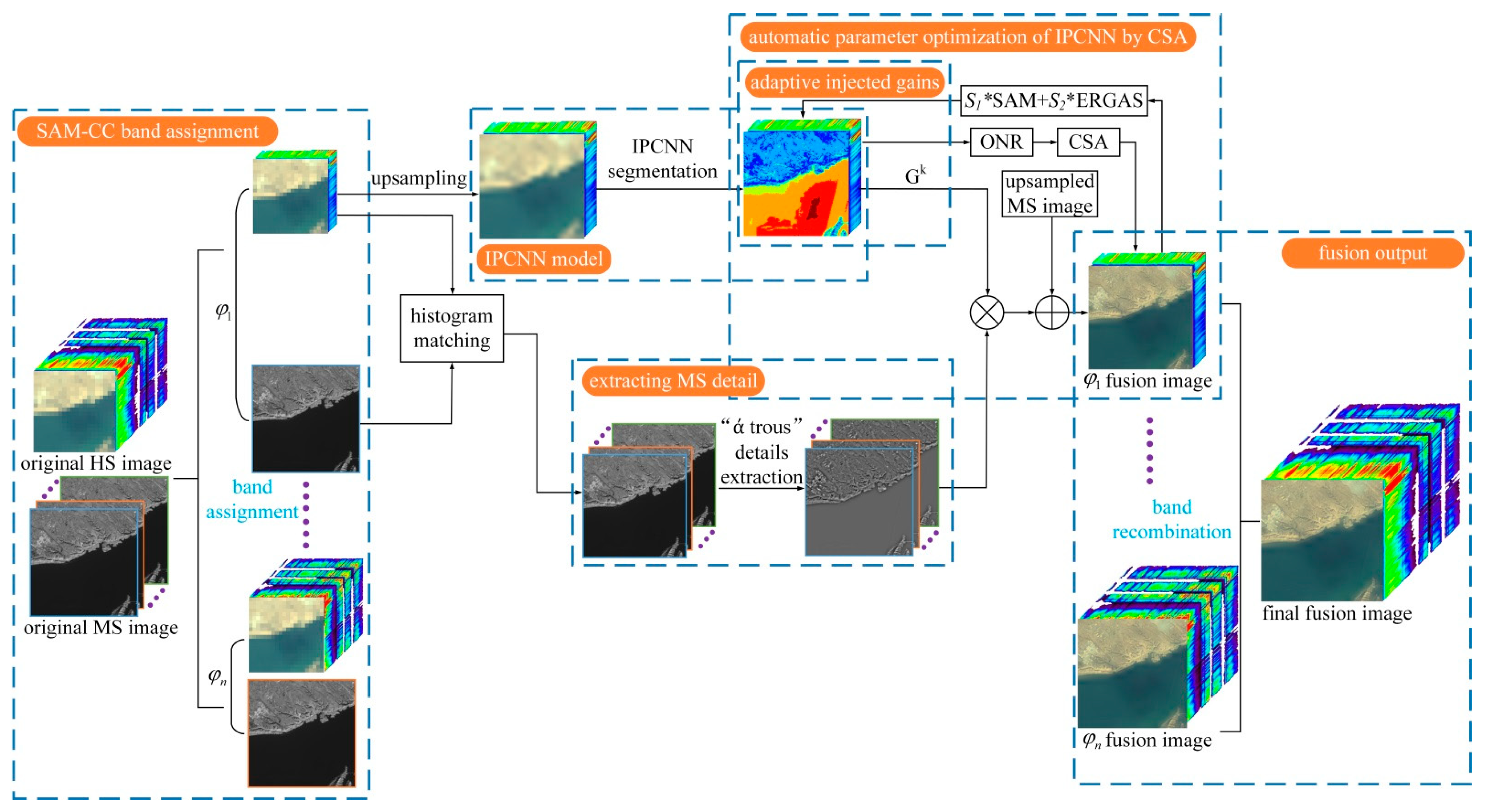
The CSA algorithm is a meta-heuristic method proposed by Malik [39]. The model imitates the socially intelligent synergistic behavior of chameleons when foraging and capturing food near woods, swamps, and deserts. It is a bio-optimization algorithm for finding the global optimum of nonlinear, nonconvex, and other complex problems, which may prevent entrapment in the local optimum.

The principle of CSA is shown in Figure 2. The algorithm mathematizes the behavioral stages of a chameleon in looking for food, which include initializing the starting position, tracking the prey from a distance, locating the prey by eye rotation, and catching the prey with a high-velocity sticky tongue.

3. Proposed Method

In order to tackle the problem of spectral distortion and fuzzy spatial details in HS sharpening, we propose a novel adaptively optimized PCNN fusion algorithm. The flowchart of the proposed HS sharpening algorithm is shown in Figure 3, which contains the following modules: (1) the SAM-CC band assignment part; (2) the improved PCNN (IPCNN) model part; (3) the automatic parameter optimization of IPCNN by CSA part; (4) the extracting MS detail part; (5) the adaptive injected gains part; (6) the fusion output part.

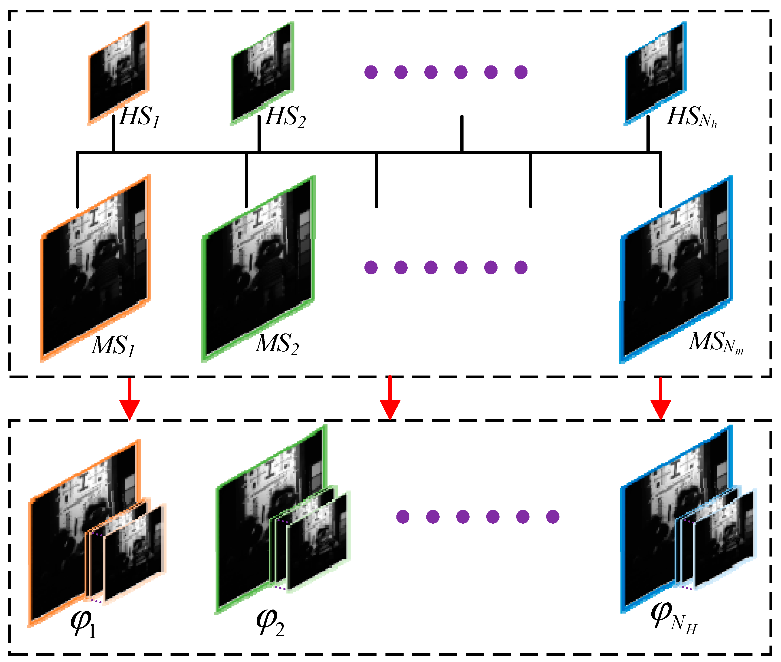
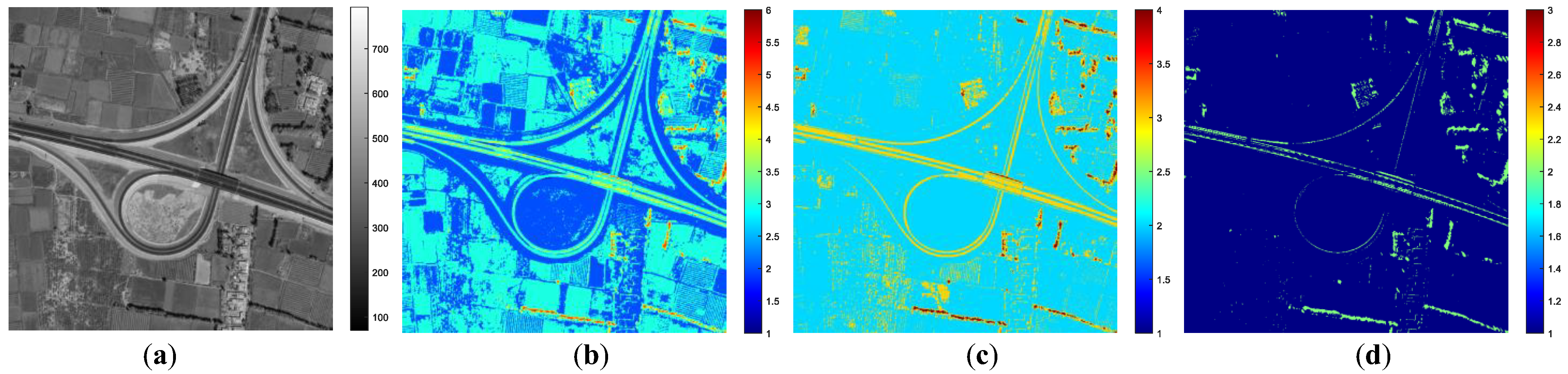
3.1. SAM-CC Band Assignment Block

In contrast to the multi-to-single band assignment in the pansharpening problem, HS sharpening is a multiband-to-multiband fusion. Thus, as shown in Figure 4, correctly assigning each HS band to the MS band is an essential procedure before the actual fusion operation, i.e., the choice of which band in the MS imagery can be used to sharpen the corresponding HS bands plays a crucial role. Classical band selection methods include the minimum spectral distance (MSD) assignment algorithm, the maximum cross-correlation (CC) assignment algorithm, and the minimum spectral distortion (SAM) assignment algorithm [24]. Since the optimal band selection is challenging for any single criterion, we propose a joint band selection algorithm using both the SAM and CC indices (SAM-CC) in order to group the HS bands more accurately.

Let H = {H}_{h = 1,…, Nh}, stands for the HS images and M = {M}_{m = 1,…, Nm}, represents the MS images, where h and m are the band numbers of HS and MS, respectively. N_h and N_m refer to the total number of bands of HS and MS. The proposed SAM-CC criterion is represented as Equation (6).

$$SAM\text{-}CC\left(H_h,M_m^r\right)=\arg \underset{m}{\min }\left(E-CC\left(H_h,M_m^r\right)\right)\times SAM\left(H_h,M_m^r\right)$$

(6)

$$CC\left(H_h,M_m^r\right)=\frac{〈H_h,M_m^r〉}{\sqrt{〈H_h,H_h〉〈M_m^r,M_m^r〉}}$$

(7)

$$SAM\left(H_h,M_m^r\right)=\left(\frac{1}{N_h}\right){\displaystyle \sum _{h=1}^{N_h}\arccos (\frac{〈H_h,M_m^r〉}{\parallel H_h\parallel .\parallel M_m^r\parallel })}$$

(8)

where E is a unit matrix with size N_M × N_H. The symbol $<·>$ indicates the inner product operation. The symbol $\Vert ·\Vert$ stands for the l₂ norm. r refers to the spatial resolution ratio of HS to MS. ${\mathbf{M}}_{\mathbf{j}}^{\mathbf{r}}$ represents the low-pass filtered down-sampled image of M_j.

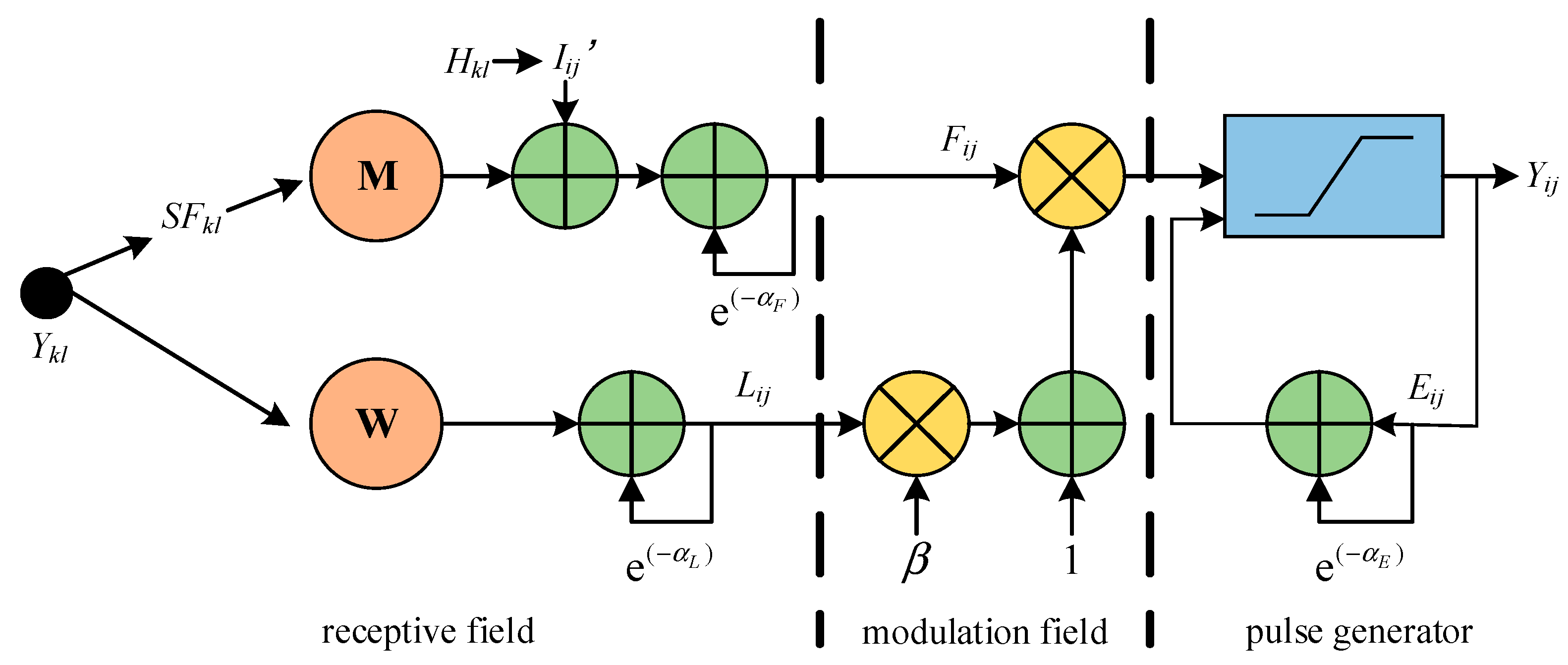
3.2. Improved PCNN Model

To make the PCNN model more suitable for HS sharpening, we propose an IPCNN model in the paper. In the standard PCNN model, the feeding input F stands for the accumulative influence of the external stimuli. Nonetheless, the human eyes are more sensitive to the edges and orientations rather than individual pixels within an image. Therefore, a new feeding input SF is designed in the IPCNN model, which considers the local neighborhood differences in both the horizontal and vertical directions. The SF is calculated in Equations (9)–(11).

$$S{F}_{ij}=\sqrt{R{F}_{ij}^2+C{F}_{ij}^2}$$

(9)

$$R{F}_{ij}=\sqrt{\frac{1}{M_1\times M_2}{\displaystyle \sum _{i=1}^{M_1}{\displaystyle \sum _{j=2}^{M_2}{[F\left(i,j\right)-F\left(i,j-1\right)]}^2}}}$$

(10)

$$C{F}_{ij}=\sqrt{\frac{1}{M_1\times M_2}{\displaystyle \sum _{i=2}^{M_1}{\displaystyle \sum _{j=1}^{M_2}{[F\left(i,j\right)-F\left(i-1,j\right)]}^2}}}$$

(11)

where RF_ij denotes the row difference of the two neighboring feeding inputs F via the local rectangular window M₁ × M₂, and CF_ij indicates the column difference. After performing a number of experiments, we take the window size to be 5 × 5. Furthermore, I_ij′ is designed to strengthen the impact of the local neighborhood, which is given by Equation (12).

$$I_{ij}^{\prime }=\left(\frac{1}{2}\right)\left(H_{ij}+\sqrt{\frac{1}{M_1\times M_2}{\displaystyle \sum _{i=1}^{M_1}{\displaystyle \sum _{j=1}^{M_2}{H}_{ij}^2}}}\right)$$

(12)

where H_ij refers to the pixel value of the upsampled HS in row i and column j.

After modeling the new SF and I′, the proposed IPCNN neuron model is illustrated in Figure 5. The IPCNN model has the following advantages compared to the standard PCNN: (1) the IPCNN model utilizes the spatial difference of the neighborhoods to stimulate the feeding input F_ij of the neuron, which can describe the local detail features; (2) the external stimuli I_ij considers the influence of the surrounding pixels towards the central pixels.

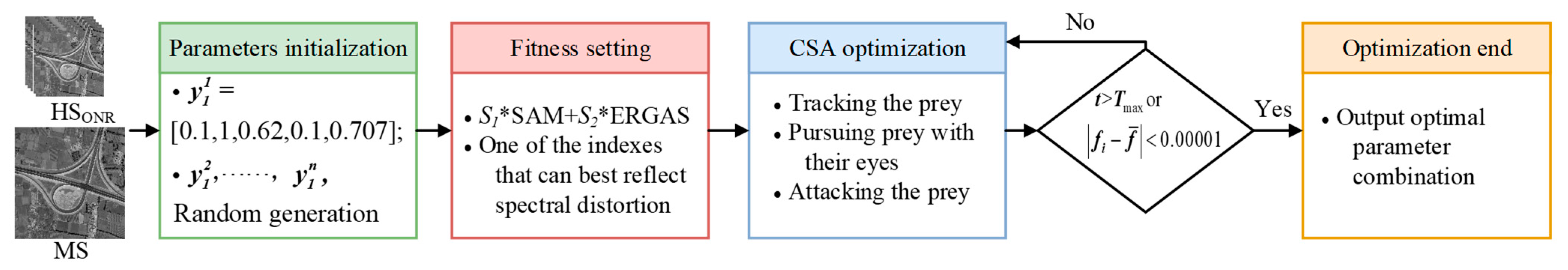
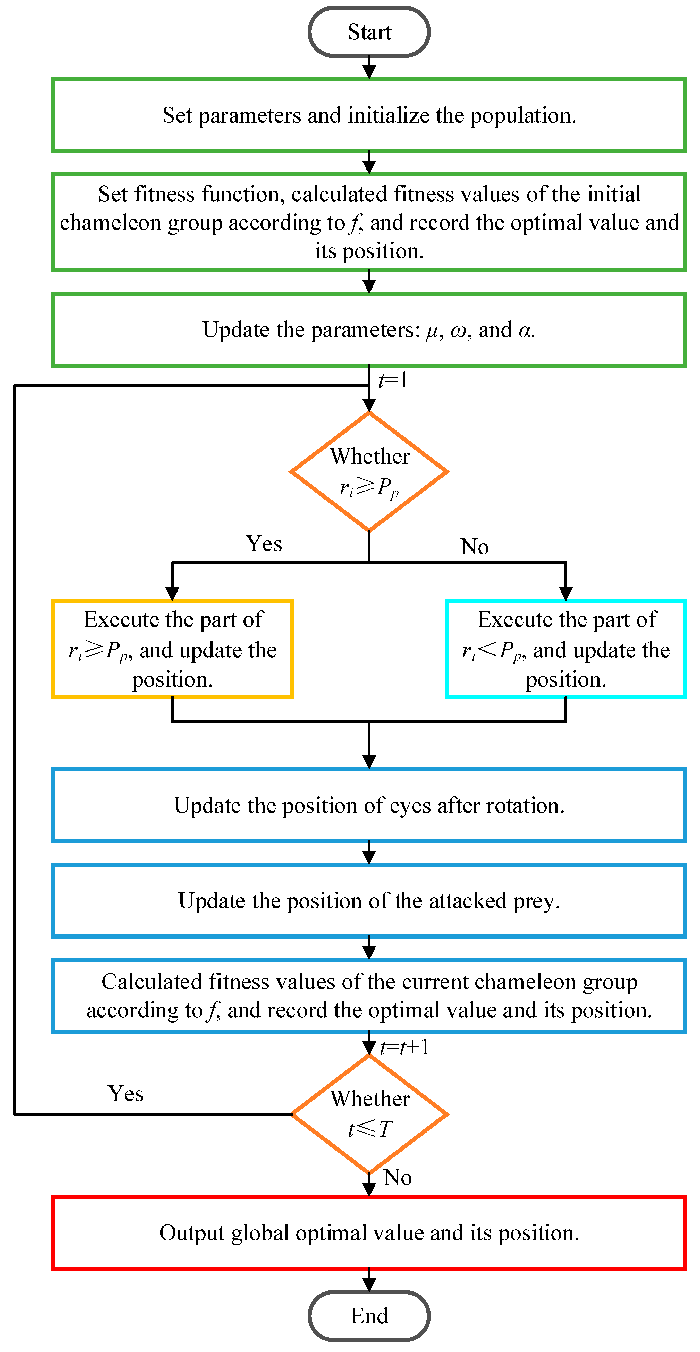
3.3. Automatic Parameter Optimization of IPCNN by CSA

Similar to the standard PCNN, the setting of appropriate parameters (i.e., α_F, α_L, α_E, β) of the IPCNN model is most critical. As shown in Figure 6, different combinations of IPCNN parameters will lead to different segmentation results for the same input image. If there are too many segmentation pieces, the segmentation regions will be too small and will further affect the accuracy and complexity of the statistical computation of subsequent injection weights. Conversely, if the number of image segmentation pieces is too few, it is impossible to distinguish each region or to take advantage of the characteristics of each region. So, different parameters can lead to different segmentation results, and different segmentations will have corresponding impacts on the final fusion results. Most researchers choose to simplify the PCNN model or to use the manually set uniform parameters for the different images. However, fixed parameters for different input images do not lead to the optimal fusion results for all images. Thus, we propose a CSA-based optimization approach for setting IPCNN parameters α_F, α_L, α_E, β, and W, which can adaptively generate their own optimal parameters for various input images.

The IPCNN parameters need to be jointly optimized together, so the CSA is employed to automatically optimize all five IPCNN parameters. For convenience, the connection weight W is denoted as W = [w, 1, w; 1, 0, 1; w, 1, w], where w is optimized rather than the entire matrix W. The flowchart of the automatic IPCNN parameter optimization algorithm based on CSA is shown in Figure 7. Firstly, the chameleon position is initialized with the classical parameter values. Secondly, the fitness function is set as the weighted summation of spectral fidelity SAM [5] and spatial detail representation ERGAS [40]. The fitness function for the proposed optimization method is given as follows.

$$f=\frac{SA{M}_r}{ERGA{S}_r+SA{M}_r}ERGAS+\frac{ERGA{S}_r}{ERGA{S}_r+SA{M}_r}SAM$$

(13)

$$ERGAS\left(FH,F\right)=100\frac{h}{l}\sqrt{\frac{1}{N_h}{\displaystyle \sum _{h=1}^{N_h}{\left(\frac{RMS{E}_h}{{\mu }_h}\right)}^2}}$$

(14)

$$SAM\left(FH,F\right)=\arccos \left(\frac{〈f{h}_j,f_j〉}{\parallel f{h}_j{\parallel }_2\parallel f_j{\parallel }_2}\right)$$

(15)

where FH denotes the reference imagery, and F refers to the fusion imagery. SAM_r and ERGAS_r stand for the ranges of SAM and ERGAS. h and l indicate the spatial resolutions of the MS and HS imagery, respectively. u_h indicates the mean value of the hth band of the reference imagery. <·> means the inner product. ‖·‖₂ refers to the second-order norm operation.

Since there are too many bands in the HS image, directly optimizing the parameters for all bands will be time-consuming. Now that the adjacent HS bands acquired by the SAM-CC band assignment method are usually strongly correlated, it would be more efficient to obtain optimized parameters by only using the representative bands of each group. Wang et al. proposed a HS band selection method with optimal domain reconstruction [41], which can adaptively achieve the optimal neighborhood reconstruction (ONR) to find the subsets of bands that can best represent the HS image. Thus, the ONR band selection method is used before IPCNN parameter optimization. In addition, the method can also reduce the impacts of noisy bands by taking advantage of the characteristics of neighborhood bands.

To be more efficient, the optimal IPCNN parameters are generated with the representative bands of HS images. Other HS bands could utilize these parameters as long as both bands are very similar to each other. Representative bands from each group are chosen by the ONR method. If there are more than five HS bands in each group, five of these are then selected using ONR to compose the optimal subset of bands. Otherwise, all of the bands from the original HS within the group are retained. Equation (16) is defined to express the procedure.

$$H_{{\phi }_i}={\left\{H_j\right\}}_{j\in {\phi }_i}\stackrel{\mathrm{ONR}\mathrm{band}\mathrm{selection}}{\to }{H}_{{\varphi }_i}=\left\{\begin{array}{l}{\left\{H_{jj}\right\}}_{jj\in {\varphi }_i} j>5,jj=5\\ {\left\{H_j\right\}}_{j\in {\phi }_i} j\le 5\end{array}\right.$$

(16)

3.4. Extracting MS Details

The multiscale analysis has demonstrated excellent capability in RS image fusion. The “atrous” wavelet transform is an undecimated multiscale analysis method, which is widely used to address image fusion issues due to its fast decomposition and reconstruction as well as the richer extracted details. For each histogram-matched MS band M_hm (matched by HS image), the “atrous” wavelet decomposition is performed to extract the spatial details from the multispectral imagery. After wavelet decomposition, the low-frequency component stands for the approximate image, and the high-frequency component indicates the noise and the local features. After setting the high-frequency components to zero, the low-frequency MS imagery M_L is then realized via wavelet reconstruction. Finally, the spatial detail information M_d is obtained through Equation (17).

$$M_d=M_{hm}-M_L$$

(17)

3.5. Adaptive Injected Gains

The HS imagery is divided into different irregular segmentation regions by the proposed CSA-based IPCNN segmentation algorithm. The injected gains are, therefore, calculated in each irregular region. The overall steps of the adaptive gain approach are described as follows:

(1)

Initialize IPCNN. Let V_F = 0.5, V_L = 0.2, V_E = 20, Y [0] = L [0] = U [0] = 0, E [0] = V_E.

(2)

Optimize IPCNN parameters α_F, α_L, α_E, β, and W using the CSA-based IPCNN optimization algorithm.

(3)

Obtain the irregular segmentation region of the IPCNN model in the current iteration n. And calculate the injected gain G^k[n] according to Equation (20).

$$\begin{array}{l}{R}_{ij}[n]=\left\{\begin{array}{l}\frac{\mathrm{cov}\left(H_k^u\left(i,j\right),M_L\left(i,j\right)\right)}{\mathrm{cov}\left(M_L\left(i,j\right),M_L\left(i,j\right)\right)}\hspace{1em}if Y_{ij}\left. [n\right]\ne 0\\ 0\hspace{1em}\hspace{1em}\hspace{1em}\hspace{1em}\hspace{1em}\hspace{1em} \mathrm{o}therwise\end{array}\right.\\ \end{array}$$

(18)

$$g_{{}_{ij}}^k=corr\left(H_{{}_k}^u\left(i,j\right),M_L\left(i,j\right)\right)\frac{std(H_h)}{std(M_m)}$$

(19)

$$G_{{}_{ij}}^k[n]=\left\{\begin{array}{l}{g}_{ij}^k\frac{std\left(H_{{}_k}^u\left(i,j\right)\right)}{std\left(M_L\left(i,j\right)\right)}\hspace{1em}if R_{ij}[n]>0 and Y_{ij}[n]\ne 0\\ 1\hspace{1em}\hspace{1em}\hspace{1em}\hspace{1em}\hspace{1em}otherwise\end{array}\right.$$

(20)

where (i, j) stands for the pixel coordinates of the imagery. H_k^u denotes the upsampled image of HS, and M_L indicates the low-resolution version of the MS imagery. Y[n] refers to the activated neurons in the current iteration. R is the correlation ratio between the HS and MS imagery. corr(A, B) represents the correlation coefficient between matrix A and matrix B. cov(A, B) denotes the covariance between matrix A and matrix B. std(A) refers to the standard deviation of A.

3.6. Fusion Output

The final fusion result can be calculated by Equation (21).

$$F{H}_k=H_k^u+{\mathrm{G}}^{\mathrm{k}}{M}_d$$

(21)

where FH_k denotes the high-resolution HS fusion image.

The fusion pseudo-code of the proposed HS sharpening algorithm (Algorithm 1) is described as follows.

Algorithm 1 AT-AIPCNN (“atrous” transform-adaptive IPCNN) method

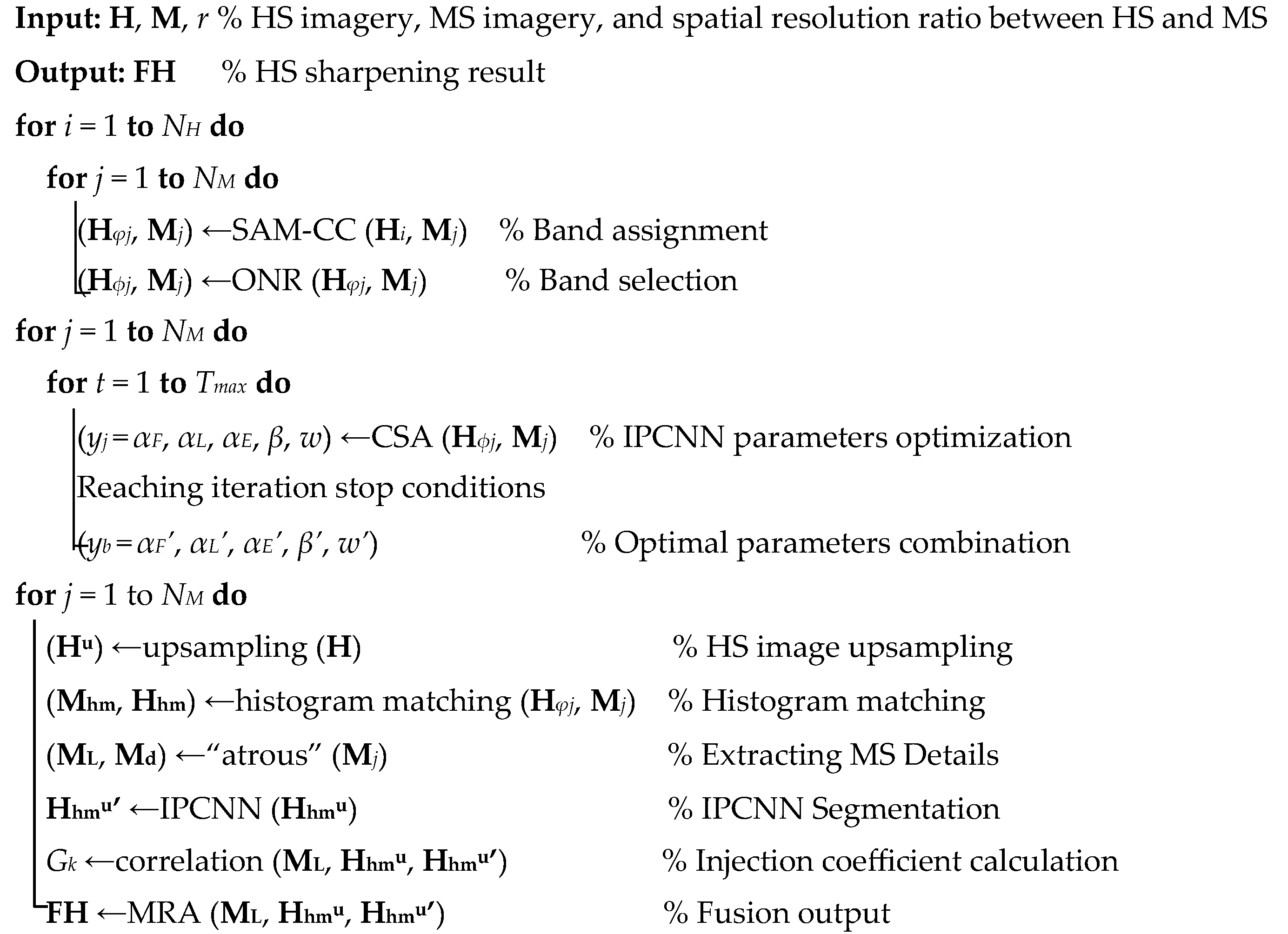
4. Experimental Results

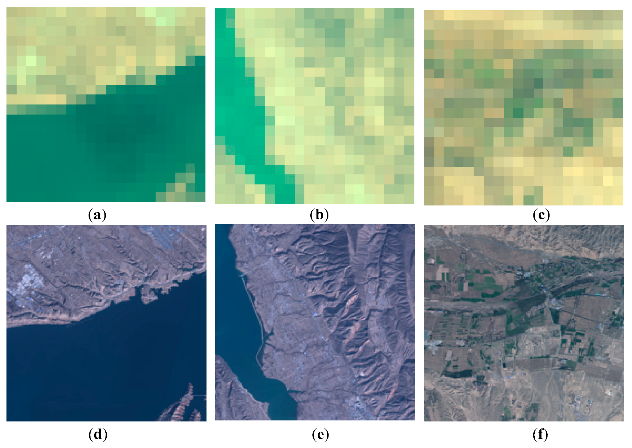
4.1. Datasets

Three real datasets captured from the ZY1-02D and GF-2 satellites are utilized to test the validity of the proposed method. The HS sensor AHSI of the ZY1-02D satellite, which works in the spectral range from the visible to the short-wave infrared (with the wavelength from 395 nm to 2500 nm), provides 166 HS bands with a spatial resolution of 30 m. The GF-2 satellite captures four multispectral bands with a spatial resolution of 3.4 m, spanning the spectral range from the visible to the near-infrared (450–890 nm). For HS sharpening application, HS images from the ZY1-02D sensor would need to be sharpened to the spatial resolution of MS imagery of the GF-2 sensor. Thus, dataset1 consists of imagery taken over the Liujiaxia reservoir in China from the ZY1-02D and GF-2 sensors, which mainly include the lake and the village. Dataset2 stands for the suburban area of Linxia City in China, mainly containing mountainous terrain. The dataset3 is the farmland area of Yongchang City in China, which primarily includes farmland, mountains, and buildings. The original images of the three datasets are shown in Figure 8.

4.2. Experimental Setup

In the experiments, most program code is executed with matlab2020a on the Intel CPU Core i7-13700K and NVIDIA GPU GeForce GTX 3090. The number of chameleon populations is set to 20 in the CSA-based IPCNN adaptive optimization, and the maximum number of iterations is set to 30.

Nine classical and competitive methods of different sharpening categories are compared with the proposed approach, i.e., the Gram-Schmidt adaptive (GSA) algorithm [12], the smoothing filtered-based intensity modulation (SFIM) algorithm [42], the generalized Laplacian pyramid (GLP) algorithm [43], the CNMF algorithm [26], the nonlocal sparse tensor factorization (NLSTF) algorithm [27], the NLSTF_SMBF algorithm [27], the HYSURE algorithm [44], the fast fusion based on Sylvester equation (FUSE) algorithm [45], and the UDALN algorithm [46]. Among which, GSA, SFIM, and GLP are owned by the classical pansharpening methods, GSA belongs to the CS methods, SFIM and GLP are the MRA method, CNMF belongs to the matrix decomposition methods, NLSTF and NLSTF_SMBF are owned by tensor decomposition categories, while the HYSURE and FUSE belong to Bayesian-based methods. In addition, GSA, SFIM, and GLP do not require any parameter setting. The main parameters for the NLSTF and NLSTF_SMBF methods are set according to

Table 1. Main parameter settings of NLSTF/NLSTF_SMBF methods.

Method	Main Parameters
NLSTF/NLSTF_SMBF	The atomic numbers for three different dictionaries: lW = 10, lH = 10, lS = 14. Parameters of sparse regularization: λ = 10−6, λ1 = 10−5, λ2 = 10−5, λ3 = 10−6. Cluster scaling parameter: K = 151. The spectral response matrix R was estimated by HYSURE [44].

, and the parameters of other comparative approaches are set to be the same as in the literature [47]. The UDALN is implemented in PyTorch, and the parameter settings are the same as in the literature [46].

The performance of the proposed HS sharpening approach is evaluated by eight complementary quantitative indices to verify the spectral and spatial qualities of the fusion imagery, such as the peak signal-to-noise ratio (PSNR) [47], the root mean square error (RMSE) [48], the error relative global adimensionnelle de synthèse (ERGAS) [40], the spectral angle mapper (SAM) [5], the structural similarity index measurement (SSIM) [49,50], the universal image quality index (UIQI) [48], the inter-correlation (CC) [51], and the degree of distortion (DD) [52]. The ideal values for RMSE, ERGAS, SAM, and DD are 0, whereas 1 for SSIM, UIQI, and CC. Moreover, the ideal value for PSNR is positive infinity.

PSNR measures the spatial similarity between the fusion imagery and the reference imagery. In general, the larger the PSNR, the more spatially similar the fusion imagery is to the reference imagery. The PSNR is defined as:

$$PSNR\left(FH,F\right)=\frac{1}{N_h}{\displaystyle \sum _{h=1}^{N_h}{\log }_{10}\left(\frac{\max {\left(F{H}_h\right)}^2}{\frac{1}{L}{\displaystyle \sum _{\mathrm{j}=1}^L{\left(F{H}_{hj}-F_{hj}\right)}^2}}\right)}$$

(22)

where FH denotes the reference imagery, and F refers to the fusion imagery. h stands for the band number, while N_h indicates the total number of all bands. log10(⸳) represents the logarithm function with base 10. FH_h denotes the hth band of the reference imagery. max(⸳) denotes the maximum value. L denotes the total number of pixels per band. FH_hj denotes the jth pixel of the hth band of the reference imagery, and F_hj stands for the jth pixel of the hth band of the fusion image.

RMSE refers to the measure of deviation between two images. The RMSE is defined as:

$$RMSE\left(FH,F\right)=\sqrt{\frac{\parallel FH,F{\parallel }_F^2}{T}}$$

(23)

where T stands for the total pixel number of the reference imagery.

ERGAS is a comprehensive index that reflects both spectral distortions and spatial detail differences. The ERGAS can be computed through Equation (14). SAM calculates the similarity of the spectral vectors. The smaller one indicates that the spectrum is better maintained. The SAM index of two images FH and F is computed as Equation (15). UIQI measures the similarity in terms of the brightness and contrast. For the window, a × b, Q is defined as:

$$Q\left(a,b\right)=\frac{4{\mu }_a{\mu }_b}{{\mu }_a^2+{\mu }_b^2}\frac{{\sigma }_{a,b}^2}{{\sigma }_a^2+{\sigma }_b^2}$$

(24)

where μ_x and ${\sigma }_x^2$ denote the expectation and variance of x, respectively, and ${\sigma }_{x,y}^2$ represents the covariance of x and y.

Then, the UIQI can be computed through the following formula:

$$UIQI\left(FH,F\right)=\frac{1}{N_h}{\displaystyle \sum _{h=1}^{N_h}Q(F{H}_h,F_h)}$$

(25)

SSIM compares the structural similarities between two images, which indicate the luminance distortion, the contrast distortion, and the structural distortion. Its formula is described in Equations (26) and (27).

$$SSIM\left(FH,F\right)=\frac{1}{N_h}{\displaystyle \sum _{h=1}^{N_h}SSIMS}\left(F{H}_h,F_h\right)$$

(26)

$$SSIMS\left(a,b\right)=\frac{\left(2{\mu }_a{\mu }_b+C_1\right)\left({\sigma }_a{\sigma }_b+C_2\right)}{\left({\mu }_a^2+{\mu }_b^2+C_1\right)\left({\sigma }_a^2+{\sigma }_b^2+C_2\right)}$$

(27)

where C₁ and C₂ are infinitesimal small constants to ensure stability.

DD is an indicator to verify the quality of the fusion spectra. The smaller the value, the better the spectral retention. If the DD is equal to 0, there is no spectral distortion. Its calculation formula is shown in Equation (28).

$$DD\left(FH,F\right)=\frac{1}{T}\parallel vec\left(FH\right)-vec\left(F\right){\parallel }_1$$

(28)

where T denotes the total pixel number of the reference imagery. vec(x) represents matrix x as a vector, and ‖ ‖₁ is the one-order norm operation.

CC represents the spatial correlation between two images, which measures the geometric distortion of the fusion imagery. It is calculated as follows:

$$CC\left(FH,F\right)=\frac{1}{N_h}{\displaystyle \sum _{h=1}^{N_h}CCS\left(F{H}_h,F_h\right)}$$

(29)

$$CCS\left(a,b\right)=\frac{{\displaystyle \sum _{i=1}^H{\displaystyle \sum _{j=1}^W\left(a_{ij}-{\mu }_a\right)\left(b_{ij}-{\mu }_b\right)}}}{\sqrt{{\displaystyle \sum _{i=1}^H{\displaystyle \sum _{j=1}^W{\left(a_{ij}-{\mu }_a\right)}^2{\left(b_{ij}-{\mu }_b\right)}^2}}}}$$

(30)

where X_h refers to the hth band of X, and μ_x indicates the mean value of x.

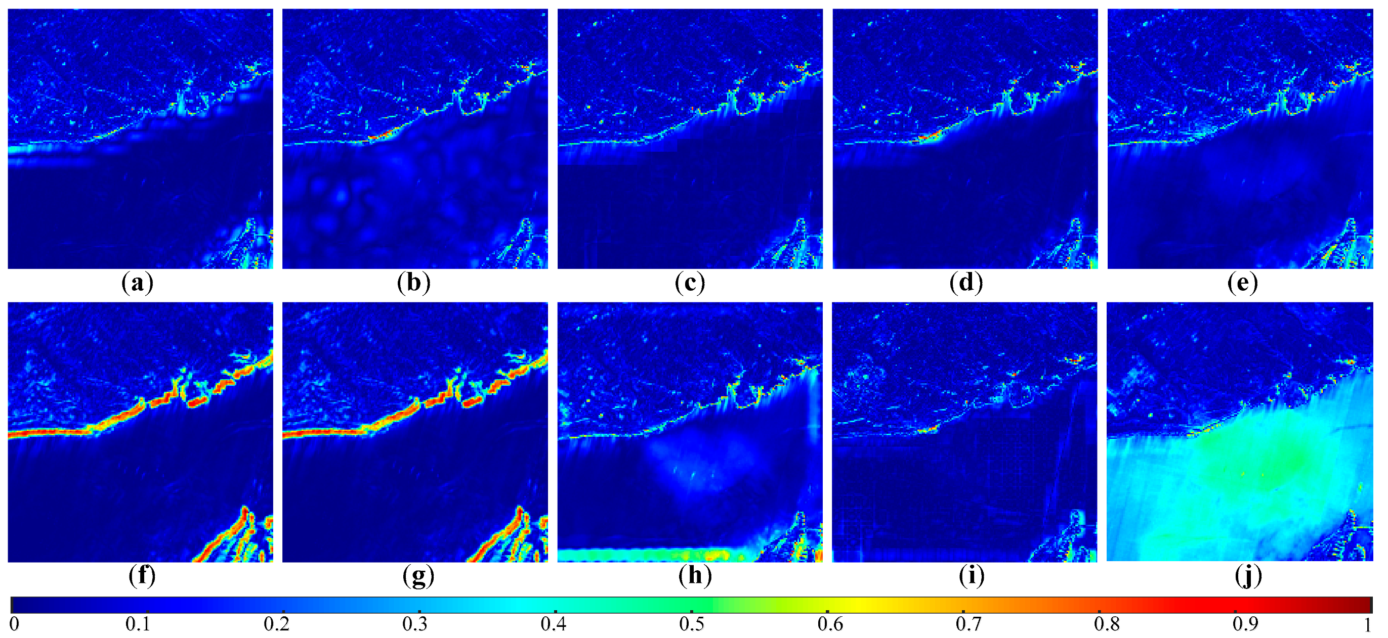
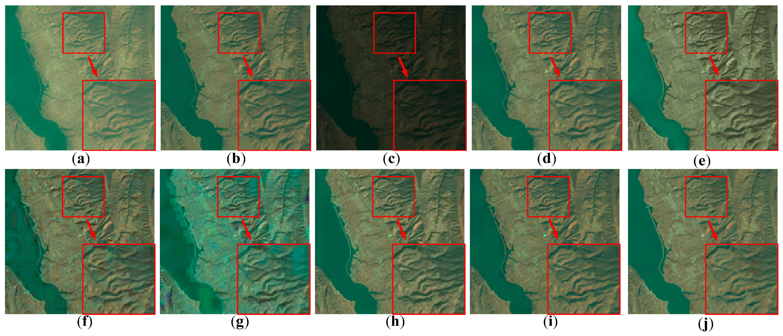
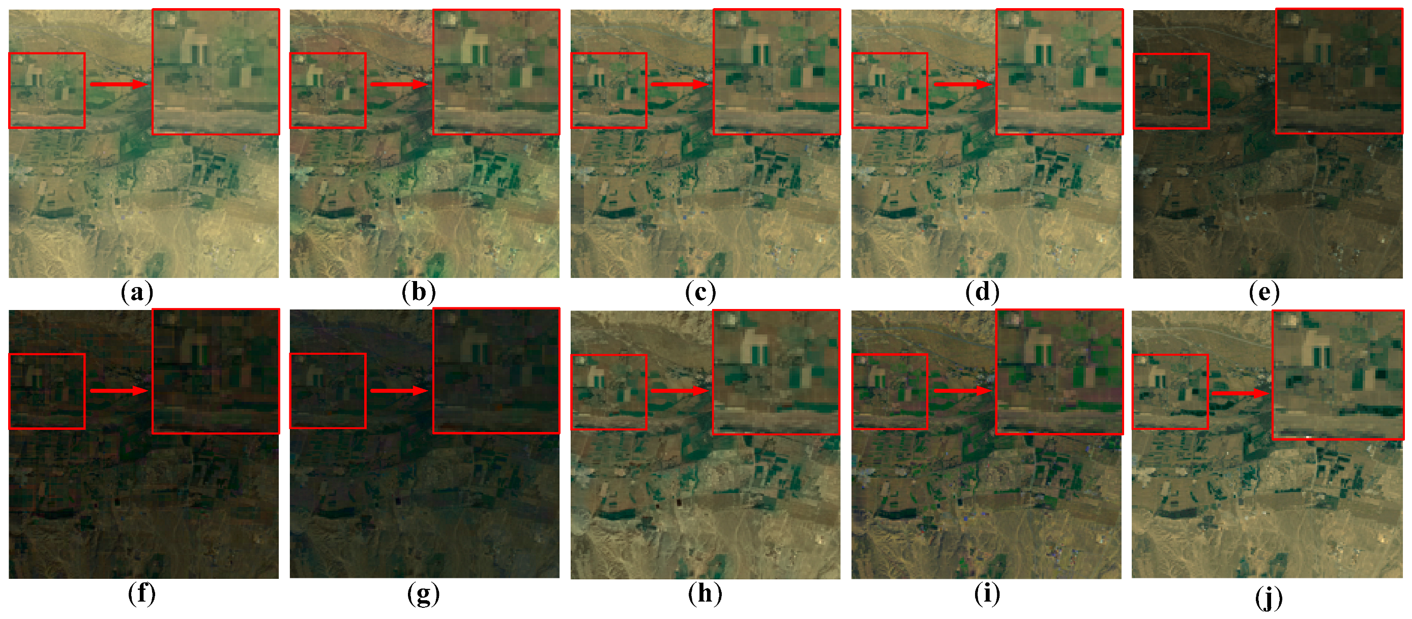
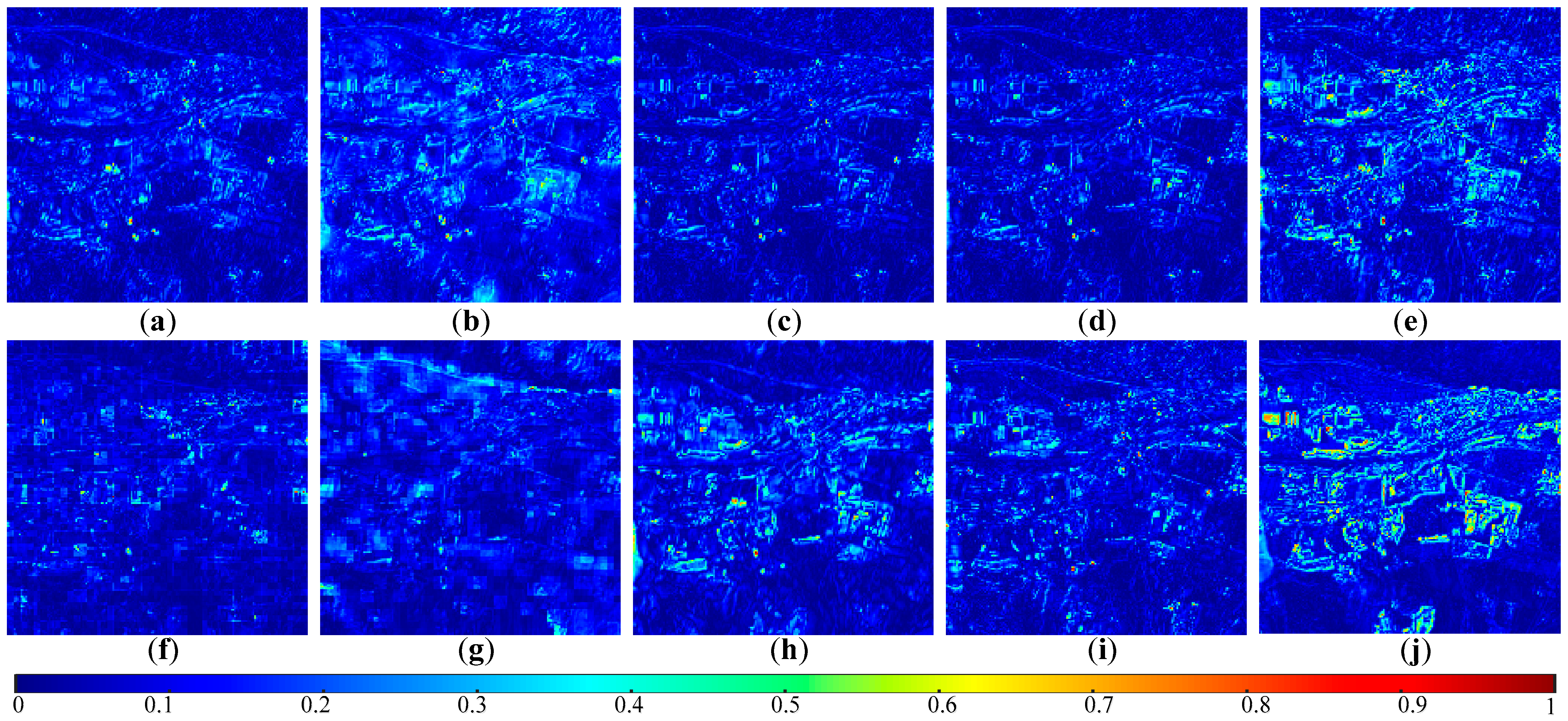
4.3. Experimental Results

The first experiment is conducted on the Liujiaxia dataset. The fusion results are shown in Figure 9, in which the local area is enlarged for convenient observation. As can be seen from Figure 9, the color of the GSA, SFIM, GLP, CNMF, HYSURE, UDALN, and FUSE methods appear to be dark. Our proposed method, NLSTF and NLSTF_SMBF methods, perform best in spectral preservation; nevertheless, the details of both the NLSTF and NLSTF_SMBF methods are blurred into chunks. Figure 10 presents the SAM error maps of the fusion images in all 166 bands with the Liujiaxia dataset. It is noted that the spectral distortion for all methods primarily occurs at the reservoir-mountain boundary, of which NLSTF and NLSTF_SMBF exhibit the largest aberration. Besides, UDALN has larger distortions in the reservoir area, and the proposed method, SFIM, and GLP perform better in the SAM error maps. Furthermore, quantitative assessments with the Liujiaxia dataset are shown in

Table 2. Quantitative evaluation results of the Liujiaxia dataset.

Method	PSNR (dB)	RMSE	ERGAS	SAM (°)	UIQI	SSIM	DD	CC
Proposed	37.6677	5.0560	1.2971	1.5961	0.7252	0.9296	2.3748	0.9863
GSA	27.6248	17.2337	5.1195	2.1357	0.5535	0.8875	11.6032	0.9767
SFIM	25.8724	21.2343	6.8882	1.7852	0.5902	0.8613	14.6026	0.9768
GLP	25.6146	21.8812	7.2056	1.7573	0.5920	0.8588	15.0508	0.9777
CNMF	26.7564	18.9197	5.8796	2.1720	0.4619	0.8707	12.8621	0.9653
NLSTF	26.7253	18.3908	4.4832	5.3202	0.3553	0.7393	11.5977	0.8935
NLSTF_SMBF	25.4524	19.5991	7.4406	9.6997	0.2621	0.6833	12.1336	0.8094
HYSURE	27.9512	16.5909	4.8475	2.2759	0.4725	0.8862	11.2004	0.9685
FUSE	23.1458	29.1700	11.5544	3.7671	0.4466	0.7746	20.1469	0.9606
UDALN	30.1948	13.0902	3.1310	6.7527	0.4611	0.8917	8.4485	0.9555

The best result is in bold, and the second best is underlined.

. It is clear from Table 2 that the proposed method obtains the best performance across all quantitative metrics, which demonstrates the superiority of the proposed method with respect to spectral preservation and spatial details.

The fusion results with the Linxia dataset are shown in Figure 11. As can be seen, the large color difference and block blur are presented in the NLSTF and NLSTF_SMBF fusion methods. Moreover, the SFIM fusion image appears dark. GSA algorithm, as a kind of CS method, has greater spectral distortion, while MRA methods, such as SFIM and GLP, have less spatial detail. Furthermore, the proposed method, GSA, and UDALN, have fine spatial detail information. In addition, the spectra of the proposed method are the closest to the ground-truth image in subjective visualization. Figure 12 shows the SAM error maps of all the fusion results with the Linxia dataset. As can be seen from Figure 12, spectral distortion is more likely to occur in the ridge area and in the land-lake boundary. Although the SFIM method has less spectral distortion in most regions, it exhibits larger errors in some local areas (top left corner and bottom left of Figure 12d). NLSTF and NLSTF_SMBF appear to have more spectral distortion, whereas the proposed method performs well.

Table 3. Quantitative evaluation results of the Linxia dataset.

Method	PSNR (dB)	RMSE	ERGAS	SAM (°)	UIQI	SSIM	DD	CC
Proposed	36.2331	5.7254	0.9960	1.9634	0.8498	0.9067	3.4608	0.9645
GSA	27.7164	16.0083	3.0327	2.6527	0.8158	0.8716	12.4741	0.9393
SFIM	17.7201	52.0659	22.7315	2.5678	0.3656	0.5387	42.0473	0.9452
GLP	29.1091	13.5721	2.4955	2.3762	0.8256	0.8826	10.5857	0.9526
CNMF	29.4453	12.4878	2.3389	2.8221	0.7854	0.8723	8.9418	0.8916
NLSTF	26.7873	16.4622	3.5301	4.5579	0.6711	0.7826	12.6480	0.8645
NLSTF_SMBF	22.4454	27.2926	9.9383	13.5531	0.4817	0.6763	20.5441	0.7075
HYSURE	29.1139	13.4809	2.4710	2.5469	0.8084	0.8665	10.3741	0.9299
FUSE	27.7103	16.0556	3.0428	2.8151	0.7959	0.8657	12.5806	0.9403
UDALN	28.3250	13.5625	2.5555	2.7875	0.7535	0.8709	10.3336	0.8834

The best result is in bold, and the second best is underlined.

gives the quantitative evaluation results of the Linxia dataset, which demonstrates that our method achieves the best indicator results.

Figure 13 presents the fusion results of the Yongchang dataset. From Figure 13, we can see that the color error occurred in the fusion result of the CNMF, NLSTF, and NLSTF_SMBF methods. In addition, The SAM error maps of the Yongchang dataset are shown in Figure 14. We note from Figure 14 that the proposed method has the least amount of spectral distortion at the edges, which is also verified by

Table 4. Quantitative evaluation results of the Yongchang farmland area data set.

Method	PSNR (dB)	RMSE	ERGAS	SAM (°)	UIQI	SSIM	DD	CC
Proposed	31.8816	11.0828	1.8716	4.4585	0.4979	0.6417	7.1603	0.7057
GSA	30.6948	12.9507	2.4569	5.1439	0.4744	0.6385	8.6661	0.6708
SFIM	30.4540	13.0830	2.5290	5.4665	0.4785	0.6243	8.5827	0.6538
GLP	31.4697	11.7546	2.2168	5.3264	0.4885	0.6284	7.2407	0.6606
CNMF	26.2153	21.5673	4.4503	6.3250	0.2844	0.5582	15.7905	0.4523
NLSTF	19.0226	51.3424	23.8635	12.8057	0.1418	0.3850	41.4662	0.3664
NLSTF_SMBF	19.5615	48.5621	21.1652	10.6630	0.1434	0.4451	38.9230	0.3652
HYSURE	26.1247	22.0403	4.6897	5.4368	0.4061	0.5953	16.4566	0.5652
FUSE	23.8007	29.0302	7.0905	7.2528	0.3347	0.5344	22.4866	0.5202
UDALN	27.9588	17.2212	2.9768	6.1002	0.3413	0.6091	12.1402	0.4833

The best result is in bold, and the second best is underlined.

.

4.4. Ablation Experiments

Three kinds of ablation experiments are carried out to test our three primary fusion modules, i.e., SAM-CC band assignment module, ONR band selection module, and CSA adaptive PCNN parameter module. In addition, different automatic parameter optimization strategies are also investigated.

The fusion results obtained on three different datasets with different band assignment strategies (SAM-CC, SAM, and CC) are presented in

Table 5. SAM-CC ablation.

Method	PSNR (dB)	RMSE	ERGAS	SAM (°)	UIQI	SSIM	DD	CC
SAM-CC (dataset1)	37.6677	5.0560	1.2971	1.5961	0.7252	0.9296	2.3748	0.9863
SAM (dataset1)	37.1726	5.2919	1.4142	1.7293	0.7139	0.9215	2.5195	0.9847
CC (dataset1)	37.2604	5.3198	1.3380	1.6597	0.7113	0.9237	2.5311	0.9852
SAM-CC (dataset2)	36.2331	5.7254	0.9960	1.9634	0.8498	0.9067	3.4608	0.9645
SAM (dataset2)	36.3003	5.6917	0.9988	1.9721	0.8493	0.9059	3.4370	0.9645
CC (dataset2)	35.0948	6.4739	1.1504	2.0009	0.8383	0.9017	4.2271	0.9634
SAM-CC (dataset3)	31.8816	11.0828	1.8716	4.4585	0.4979	0.6417	7.1603	0.7057
SAM (dataset3)	28.4326	16.8280	2.2748	4.1073	0.5638	0.7168	12.6765	0.7755
CC (dataset3)	31.2056	12.2060	1.9122	4.8604	0.5026	0.6967	8.1791	0.7334

The best result is in bold, and the second best is underlined.

. For the Liujiaxia dataset, our proposed SAM-CC assignment indicator performs best. Furthermore, the SAM-CC achieves better fusion results in most cases with the Linxia dataset and the Yongchang dataset, which illustrates the effectiveness of the SAM-CC band assignment.

To validate the efficiency of the ONR band selection module, we compared the fusion results of using ONR and without ONR. In order to verify the effectiveness of ONR band selection, we fused the data sets with and without ONR band selection. Comparisons of the fusion accuracy and the running time are shown in

Table 6. ONR band selection for ablation.

Method	PSNR (dB)	RMSE	ERGAS	SAM (°)	UIQI	SSIM	DD	CC	Time (s)
Using ONR (dataset1)	37.6677	5.0560	1.2971	1.5961	0.7252	0.9296	2.3748	0.9863	221.1
Without ONR (dataset1)	37.3746	5.2096	1.3166	1.6199	0.7143	0.9272	2.5202	0.9859	1937.6
Using ONR (dataset2)	36.2331	5.7254	0.9960	1.9634	0.8498	0.9067	3.4608	0.9645	132.1
Without ONR (dataset2)	36.3467	5.6366	0.9918	1.9085	0.8533	0.9082	3.3977	0.9646	1794.2
Using ONR (dataset3)	31.8816	11.0828	1.8716	4.4585	0.4979	0.6417	7.1603	0.7057	179.2
Without ONR (dataset3)	30.9860	12.2864	1.8764	4.1296	0.5532	0.7081	8.6389	0.7665	1219.2

The best result is in bold, and the second best is underlined.

. As can be seen from Table 6, the running time has been reduced by more than 84% with the ONR band selection module, while the fusion accuracy remains almost unchanged. Overall, this indicates significant time cost savings for the ONR band selection module.

In order to examine the rationality of the CSA-based parameter optimization strategy in IPCNN,

Table 7. Automatic parameter optimization ablation.

Method	PSNR (dB)	RMSE	ERGAS	SAM (°)	UIQI	SSIM	DD	CC	Time (s)
CSA (dataset1)	37.6677	5.0560	1.2971	1.5961	0.7252	0.9296	2.3748	0.9863	221.1
SSA (dataset1)	37.0112	5.4224	1.4200	1.6315	0.6999	0.9289	2.8151	0.9860	267.9
IGWO (dataset1)	37.1760	5.3224	1.3947	1.6253	0.7051	0.9291	2.7133	0.9861	394.6
EWOA (dataset1)	37.3093	5.2504	1.3730	1.6361	0.7099	0.9291	2.6281	0.9861	162.6
CSA (dataset2)	36.2331	5.7254	0.9960	1.9634	0.8498	0.9067	3.4608	0.9645	132.1
SSA (dataset2)	36.2738	5.7156	1.0086	1.9955	0.8466	0.9056	3.4595	0.9643	214.3
IGWO (dataset2)	36.2348	5.7139	1.0024	1.9743	0.8478	0.9059	3.4537	0.9640	246.4
EWOA (dataset2)	36.2304	5.7458	1.0128	2.0058	0.8473	0.9056	3.4952	0.9644	122.1
CSA (dataset3)	31.8816	11.0828	1.8716	4.4585	0.4979	0.6417	7.1603	0.7057	179.2
SSA (dataset3)	30.1932	13.5601	1.9849	4.1381	0.5554	0.7070	9.7518	0.7679	199.2
IGWO (dataset3)	30.7599	12.6262	1.9081	4.1242	0.5539	0.7080	8.9401	0.7672	280.4
EWOA (dataset3)	30.3997	13.2174	1.9643	4.1652	0.5525	0.7043	9.4456	0.7671	137.6

The best result is in bold, and the second best is underlined.

shows the comparison of the CSA fusion metrics with other three parameter optimization strategies, i.e., the sparrow search strategy (SSA) [53], the improved grey wolf optimizer (IGWO) strategy [54] and the enhanced whale optimization strategy (EWOA) [55]. As shown in Table 7, the CSA-based fusion algorithm achieves a better fusion performance as well as less time-consuming.

Table 8. CSA adaptive IPCNN parameter ablation.

Method	PSNR (dB)	RMSE	ERGAS	SAM (°)	UIQI	SSIM	DD	CC
Adaptive (dataset1)	37.6677	5.0560	1.2971	1.5961	0.7252	0.9296	2.3748	0.9863
Traditional (dataset1)	29.4710	13.8064	3.8469	1.6911	0.6480	0.9020	9.1179	0.9818
Adaptive (dataset2)	36.2331	5.7254	0.9960	1.9634	0.8498	0.9067	3.4608	0.9645
Traditional (dataset2)	34.1057	7.2630	1.2945	1.9978	0.8346	0.9043	5.0036	0.9629
Adaptive (dataset3)	31.8816	11.0828	1.8716	4.4585	0.4979	0.6417	7.1603	0.7057
Traditional (dataset3)	29.7485	14.3252	2.0709	4.2138	0.5481	0.6916	10.3473	0.7591

The best result is in bold, and the second best is underlined.

exhibits the quantitative analysis of the fusion results with and without adaptive CSA optimization to verify the impact of the CSA algorithm. Besides, the traditional IPCNN parameters are set as classical values, i.e., α_F = 0.1, α_L = 1, α_E =0.62, β = 0.1, w = 0.5. In all three datasets, the adaptive IPCNN approach is significantly superior to the traditional parameters in most cases, which indicates that the adaptive parameter optimization effectively improves the quality of the fusion images.

5. Conclusions

In the paper, a novel algorithm for HS sharpening is proposed. Firstly, the band groups are acquired by performing joint SAM-CC band matching of HS and MS assignment method, the band grouping results are obtained, and then ONR is applied to the HS images of each group to improve the efficiency for subsequent adaption. Besides, according to the characteristics of remote sensing image fusion application, an IPCNN model is proposed, which can obtain irregular injection regions of spatial details. In addition, a CSA-based IPCNN parameter optimization method is designed to achieve the optimal sharpening imagery. In summary, the proposed method is simple and easy to implement, which presents good fusion results on a variety of datasets, including reservoir, mountain, town, and river landscapes. Furthermore, several ablation experiments are also conducted to corroborate the efficiency of the proposed method.

References

1. Kokila, S.; Jayachandran, A. Hybrid Behrens-Fisher- and Gray Contrast–Based Feature Point Selection for Building Detection from Satellite Images. J. Geovisualization Spat. Anal. 2023, 7, 8. [Google Scholar] [CrossRef]
2. Zheng, Z.; Hu, Y.; Yang, H.; Qiao, Y.; He, Y.; Zhang, Y.; Huang, Y. AFFU-Net: Attention feature fusion U-Net with hybrid loss for winter jujube crack detection. Comput. Electron. Agric. 2022, 198, 107049. [Google Scholar] [CrossRef]
3. Gadea, O.; Khan, S. Detection of Bastnäsite-Rich Veins in Rare Earth Element Ores through Hyperspectral Imaging. IEEE Geosci. Remote Sens. Lett. 2023, 20, 1–4. [Google Scholar] [CrossRef]
4. Boubanga-Tombet, S.; Huot, A.; Vitins, I.; Heuberger, S.; Veuve, C.; Eisele, A.; Hewson, R.; Guyot, E.; Marcotte, F.; Chamberland, M. Thermal Infrared Hyperspectral Imaging for Mineralogy Mapping of a Mine Face. Remote Sens. 2018, 10, 1518. [Google Scholar] [CrossRef]
5. Vivone, G.; Dalla Mura, M.; Garzelli, A.; Restaino, R.; Scarpa, G.; Ulfarsson, M.O.; Alparone, L.; Chanussot, J. A New Benchmark Based on Recent Advances in Multispectral Pansharpening: Revisiting Pansharpening with Classical and Emerging Pansharpening Methods. IEEE Geosci. Remote Sens. Mag. 2020, 9, 53–81. [Google Scholar] [CrossRef]
6. Jiayuan, L.; Ai, M.; Wang, S.; Hu, Q. GRF: Guided Residual Fusion for Pansharpening. Int. J. Remote Sens. 2022, 43, 3609–3627. [Google Scholar]
7. Wu, Z.; Huang, Y.; Zhang, K. Remote Sensing Image Fusion Method Based on PCA and Curvelet Transform. J. Indian Soc. Remote Sens. 2018, 46, 687–695. [Google Scholar] [CrossRef]
8. Kong, Y.; Hong, F.; Leung, H.; Peng, X. A Fusion Method of Optical Image and SAR Image Based on Dense-UGAN and Gram–Schmidt Transformation. Remote Sens. 2021, 13, 4274. [Google Scholar] [CrossRef]
9. Garzelli, A.; Nencini, F.; Capobianco, L. Optimal MMSE pan sharpening of very high resolution multispectral images. IEEE Trans. Geosci. Remote Sens. 2008, 46, 228–236. [Google Scholar] [CrossRef]
10. Vivone, G. Robust Band-Dependent Spatial-Detail Approaches for Panchromatic Sharpening. IEEE Trans. Geosci. Remote Sens. Publ. IEEE Geosci. Remote Sens. Soc. 2019, 57, 6421–6433. [Google Scholar] [CrossRef]
11. Yang, Y.; Wan, C.; Huang, S.; Lu, H.; Wan, W. Pansharpening Based on Adaptive High-Frequency Fusion and Injection Coefficients Optimization. IEEE J. Sel. Top. Appl. Earth Obs. Remote Sens. 2023, 16, 799–811. [Google Scholar] [CrossRef]
12. Dian, R.; Li, S.; Sun, B.; Guo, A. Recent advances and new guidelines on hyperspectral and multispectral image fusion. Inf. Fusion 2021, 69, 40–51. [Google Scholar] [CrossRef]
13. Bouslihim, Y.; Kharrou, M.H.; Miftah, A.; Attou, T.; Bouchaou, L.; Chehbouni, A. Comparing Pan-sharpened Landsat-9 and Sentinel-2 for Land-Use Classification Using Machine Learning Classifiers. J. Geovisualization Spat. Anal. 2022, 6, 35. [Google Scholar] [CrossRef]
14. Burt, P.; Adelson, E. The Laplacian Pyramid as a Compact Image Code. Read. Comput. Vis. 1987, 31, 671–679. [Google Scholar]
15. Gao, W.; Xiao, Z.; Bao, T. Detection and Identification of Potato-Typical Diseases Based on Multidimensional Fusion Atrous-CNN and Hyperspectral Data. Appl. Sci. 2023, 13, 5023. [Google Scholar] [CrossRef]
16. Jindal, H.; Bharti, M.; Kasana, S.; Saxena, S. An ensemble mosaicing and ridgelet based fusion technique for underwater panoramic image reconstruction and its refinement. Multimed. Tools Appl. Available online: https://link.springer.com/article/10.1007/s11042-023-14594-9 (accessed on 8 March 2023). [CrossRef]
17. Du, C.; Gao, S. Remote sensing image fusion based on nonlinear IHS and fast nonsubsampled contourlet transform. J. Indian Soc. Remote Sens. 2018, 46, 2023–2032. [Google Scholar] [CrossRef]
18. Cheng, S.; Qiguang, M.; Pengfei, X. A novel algorithm of remote sensing image fusion based on Shearlets and PCNN. Neurocomputing 2013, 117, 47–53. [Google Scholar] [CrossRef]
19. Restaino, R.; Vivone, G.; Dalla Mura, M.; Chanussot, J. Fusion of multispectral and panchromatic images based on morphological operators. IEEE Trans. Image Process. 2016, 25, 2882–2895. [Google Scholar] [CrossRef] [PubMed]
20. Ren, C.; Liang, Y.; Lu, X.; Yan, H. Research on the soil moisture sliding estimation method using the LS-SVM based on multi-satellite fusion. Int. J. Remote Sens. 2019, 40, 2104–2119. [Google Scholar] [CrossRef]
21. Vivone, G. Multispectral and hyperspectral image fusion in remote sensing: A survey. Inf. Fusion 2023, 89, 405–417. [Google Scholar] [CrossRef]
22. Gomez, R.; Jazaeri, A.; Kafatos, M. Wavelet-based hyperspectral and multispectral image fusion. Proc. SPIE-Int. Soc. Opt. Eng. 2001, 4383, 36–42. [Google Scholar]
23. Chen, Z.; Pu, H.; Wang, B.; Jiang, G.-M. Fusion of Hyperspectral and Multispectral Images: A Novel Framework Based on Generalization of Pan-Sharpening Methods. IEEE Geosci. Remote Sens. Lett. 2014, 11, 1418–1422. [Google Scholar] [CrossRef]
24. Picone, D.; Restaino, R.; Vivone, G.; Addesso, P.; Dalla Mura, M.; Chanussot, J. Band assignment approaches for hyperspectral sharpening. IEEE Geosci. Remote Sens. Lett. 2017, 14, 739–743. [Google Scholar] [CrossRef]
25. Lu, X.; Zhang, J.; Yu, X.; Tang, W.; Li, T.; Zhang, Y. Hyper-sharpening based on spectral modulation. IEEE J. Sel. Top. Appl. Earth Obs. Remote Sens. 2019, 12, 1534–1548. [Google Scholar] [CrossRef]
26. Yokoya, N.; Yairi, T.; Iwasaki, A. Coupled Nonnegative Matrix Factorization Unmixing for Hyperspectral and Multispectral Data Fusion. IEEE Trans. Geosci. Remote Sens. 2012, 50, 528–537. [Google Scholar] [CrossRef]
27. Dian, R.; Li, S.; Fang, L.; Lu, T.; Bioucas-Dias, J.M. Nonlocal Sparse Tensor Factorization for Semiblind Hyperspectral and Multispectral Images Fusion. IEEE Trans. Cybern. 2020, 50, 4469–4480. [Google Scholar] [CrossRef]
28. Li, J.; Hong, D.; Gao, L.; Yao, J.; Zheng, K.; Zhang, B.; Chanussot, J. Deep learning in multimodal remote sensing data fusion: A comprehensive review. Int. J. Appl. Earth Obs. Geoinf. 2022, 112, 102926. [Google Scholar] [CrossRef]
29. Liu, J.; Yuan, Z.; Pan, Z.; Fu, Y.; Liu, L.; Lu, B. Diffusion Model with Detail Complement for Super-Resolution of Remote Sensing. Remote Sens. 2022, 14, 4834. [Google Scholar] [CrossRef]
30. Zhang, L.; Nie, J.; Wei, W.; Li, Y.; Zhang, Y. Deep blind hyperspectral image super-resolution. IEEE Trans. Neural Netw. Learn. Syst. 2021, 32, 2388–2400. [Google Scholar] [CrossRef]
31. Qu, Y.; Qi, H.; Kwan, C.; Yokoya, N.; Chanussot, J. Unsupervised and unregistered hyperspectral image super-resolution with mutual Dirichlet-Net. IEEE Trans. Geosci. Remote Sens. 2022, 60, 1–18. [Google Scholar] [CrossRef]
32. Li, X.; Yan, H.; Xie, W.; Kang, L.; Tian, Y. An Improved Pulse-Coupled Neural Network Model for Pansharpening. Sensors 2020, 20, 2764. [Google Scholar] [CrossRef] [PubMed]
33. Zhang, L.; Zeng, G.; Wei, J.; Xuan, Z. Multi-modality image fusion in adaptive-parameters SPCNN based on inherent characteristics of image. IEEE Sens. J. 2020, 20, 11820–11827. [Google Scholar] [CrossRef]
34. Bhagyashree, V.; Manisha, D.; Mohammad, F.; Avinash, G.; Deep, G. Saliency Detection Using a Bio-inspired Spiking Neural Network Driven by Local and Global Saliency. Appl. Artif. Intell. 2022, 36, 2900–2928. [Google Scholar]
35. Huang, C.; Tian, G.; Lan, Y.; Peng, Y.; Ng, E.; Hao, Y.; Che, W. A new pulse coupled neural network (PCNN) for brain medical image fusion empowered by shuffled frog leaping algorithm. Front. Neurosci. 2019, 13, 210. [Google Scholar] [CrossRef]
36. Panigrahy, C.; Seal, A.; Mahato, N. Fractal dimension based parameter adaptive dual channel PCNN for multi-focus image fusion. Opt. Lasers Eng. 2020, 133, 106141. [Google Scholar] [CrossRef]
37. Panigrahy, C.; Seal, A.; Gonzalo-Martín, C.; Pathak, P.; Jalal, A. Parameter adaptive unit-linking pulse coupled neural network based MRI-PET/SPECT image fusion. Biomed. Signal Process. Control 2023, 83, 104659. [Google Scholar] [CrossRef]
38. Johnson, J.; Padgett, M. PCNN models and applications. IEEE Trans. Neural Netw. 1999, 10, 480–498. [Google Scholar] [CrossRef]
39. Braik, M. Chameleon Swarm Algorithm: A Bio-inspired Optimizer for Solving Engineering Design Problems. Expert Syst. Appl. 2021, 174, 114685. [Google Scholar] [CrossRef]
40. Ren, K.; Sun, W.; Meng, X.; Yang, G.; Du, Q. Fusing China GF-5 Hyperspectral Data with GF-1, GF-2 and Sentinel-2A Multispectral Data: Which Methods Should Be Used? Remote Sens. 2020, 12, 882. [Google Scholar] [CrossRef]
41. Wang, Q.; Zhang, F.; Li, X. Hyperspectral band selection via optimal neighborhood reconstruction. IEEE Trans. Geosci. Remote Sens. 2020, 58, 8465–8476. [Google Scholar] [CrossRef]
42. Liu, J. Smoothing Filter-based Intensity Modulation: A spectral preserve image fusion technique for improving spatial details. Int. J. Remote Sens. 2000, 21, 3461–3472. [Google Scholar] [CrossRef]
43. Aiazzi, B.; Alparone, L.; Baronti, S.; Garzelli, A.; Selva, M. MTF-tailored Multiscale Fusion of High-resolution MS and Pan Imagery. Photogramm. Eng. Remote Sens. 2015, 72, 591–596. [Google Scholar] [CrossRef]
44. Simões, M.; Bioucas-Dias, J.; Almeida, L.B.; Chanussot, J. A Convex Formulation for Hyperspectral Image Superresolution via Subspace-Based Regularization. IEEE Trans. Geosci. Remote Sens. 2015, 53, 3373–3388. [Google Scholar] [CrossRef]
45. Wei, Q.; Bioucas-Dias, J.; Dobigeon, N.; Tourneret, J.-Y. Hyperspectral and Multispectral Image Fusion Based on a Sparse Representation. IEEE Trans. Geosci. Remote Sens. 2015, 53, 3658–3668. [Google Scholar] [CrossRef]
46. Li, J.; Zheng, K.; Yao, J.; Gao, L.; Hong, D. Deep Unsupervised Blind Hyperspectral and Multispectral Data Fusion. IEEE Geosci. Remote Sens. Lett. 2022, 19, 6007305. [Google Scholar] [CrossRef]
47. Yokoya, N.; Grohnfeldt, C.; Chanussot, J. Hyperspectral and Multispectral Data Fusion: A comparative review of the recent literature. IEEE Geosci. Remote Sens. Mag. 2017, 5, 29–56. [Google Scholar] [CrossRef]
48. Sara, D.; Mandava, A.K.; Kumar, A.; Duela, S.; Jude, A. Hyperspectral and multispectral image fusion techniques for high resolution applications: A review. Earth Sci. Inform. 2021, 14, 1685–1705. [Google Scholar] [CrossRef]
49. Wang, Z.; Bovik, A.C.; Sheikh, H.R.; Simoncelli, E.P. Image Quality Assessment: From Error Visibility to Structural Similarity. IEEE Trans. Image Process. 2004, 13, 600–612. [Google Scholar] [CrossRef]
50. Brunet, D.; Vrscay, E.R.; Wang, Z. On the mathematical properties of the structural similarity index. IEEE Trans. Image Process. 2011, 21, 1488–1499. [Google Scholar] [CrossRef]
51. Tian, X.; Li, K.; Zhang, W.; Wang, Z.; Ma, J. Interpretable Model-Driven Deep Network for Hyperspectral, Multispectral, and Panchromatic Image Fusion. IEEE Trans. Neural Netw. Learn. Syst. Available online: https://ieeexplore.ieee.org/document/10138912 (accessed on 31 May 2023). [CrossRef]
52. Li, S.; Dian, R.; Fang, L.; Bioucas-Dias, J. Fusing Hyperspectral and Multispectral Images via Coupled Sparse Tensor Factorization. IEEE Trans. Image Process. 2018, 27, 4118–4130. [Google Scholar] [CrossRef] [PubMed]
53. Xue, J.; Shen, B. A novel swarm intelligence optimization approach: Sparrow search algorithm. Syst. Sci. Control Eng. 2020, 8, 22–34. [Google Scholar] [CrossRef]
54. Nadimi-Shahraki, M.; Taghian, S.; Mirjalili, S. An improved grey wolf optimizer for solving engineering problems. Expert Syst. Appl. 2020, 166, 113917. [Google Scholar] [CrossRef]
55. Nadimi-Shahraki, M.; Zamani, H.; Mirjalili, S. Enhanced whale optimization algorithm for medical feature selection: A COVID-19 case study. Comput. Biol. Med. 2022, 148, 105858. [Google Scholar] [CrossRef]
Figure 1. Connection relationship diagram of PCNN.
Remotesensing 15 04205 g001
Figure 2. Flowchart of CSA. See reference [39] for all variable definitions.
Remotesensing 15 04205 g002
Figure 3. Flowchart of the proposed fusion algorithm.
Remotesensing 15 04205 g003
Figure 4. Schematic diagram of HS and MS bands grouping.
Remotesensing 15 04205 g004
Figure 5. IPCNN neuron model.
Remotesensing 15 04205 g005
Figure 6. IPCNN segmentation results under pseudo-color maps with different parameters of IPCNN. (a) Original image of GF-2 satellite sensor. (b) Classical parameters combination, [αF, αL, αE, β, w] = [0.1, 1, 0.62, 0.1, 0.707]. (c) Change the parameters αE and w, [αF, αL, αE, β, w] = [0.1, 1, 1, 0.1, 0.9]. (d) Change all parameters, [αF, αL, αE, β, w] = [0.5, 2.5, 2, 0.3, 0.9].
Remotesensing 15 04205 g006
Figure 7. Flowchart of CSA-based automatic IPCNN parameter optimization algorithm.
Remotesensing 15 04205 g007
Figure 8. The original images of three datasets. (a) HS image of Liujiaxia dataset. (b) HS image of Linxia dataset. (c) HS image of Yongchang dataset. (d) MS image of Liujiaxia dataset. (e) MS image of Linxia dataset. (f) MS image of Yongchang dataset.
Remotesensing 15 04205 g008
Figure 9. Color composite image of fusion results with Liujiaxia dataset (bands 35,14,7 are input to RGB channels respectively). (a) Proposed method. (b) GSA. (c) SFIM. (d) GLP. (e) CNMF. (f) NLSTF. (g) NLSTF_SMBF. (h) HYSURE. (i) FUSE. (j) UDALN.
Remotesensing 15 04205 g009
Figure 10. SMA error map of Liujiaxia dataset. (a) Proposed. (b) GSA. (c) SFIM. (d) GLP. (e) CNMF. (f) NLSTF. (g) NLSTF_SMBF. (h) HYSURE. (i) FUSE. (j) UDALN.
Remotesensing 15 04205 g010
Figure 11. Color composite image of fusion results with Linxia dataset (bands 35,14,7 are input to RGB channel respectively). (a) Proposed method. (b) GSA. (c) SFIM. (d) GLP. (e) CNMF. (f) NLSTF. (g) NLSTF_SMBF. (h) HYSURE. (i) FUSE. (j) UDALN.
Remotesensing 15 04205 g011
Figure 12. SMA error map of Linxia dataset. (a) Proposed method. (b) GSA. (c) SFIM. (d) GLP. (e) CNMF. (f) NLSTF. (g) NLSTF_SMBF. (h) HYSURE. (i) FUSE. (j) UDALN.
Remotesensing 15 04205 g012
Figure 13. Color composite image of fusion results of with Yongchang dataset (bands 29,19,9 are input to RGB channel respectively). (a) Proposed method. (b) GSA. (c) SFIM. (d) GLP. (e) CNMF. (f) NLSTF. (g) NLSTF_SMBF. (h) HYSURE. (i) FUSE. (j) UDALN.
Remotesensing 15 04205 g013
Figure 14. SMA error map of Yongchang dataset. (a) Proposed method. (b) GSA. (c) SFIM. (d) GLP. (e) CNMF. (f) NLSTF. (g) NLSTF_SMBF. (h) HYSURE. (i) FUSE. (j) UDALN.
Remotesensing 15 04205 g014