Abstract
Today, land and ocean observations are crucial for monitoring climate change. The method of GNSS reflectometry is an opportunistic way to provide low-cost observations of many geophysical parameters. However, although this method has been the subject of numerous research studies, work is still in progress to improve its possibilities and fields of application. This paper focuses on GNSS reflectometry using carrier phase measurements for water altimetry measurements. The difficulties in implementing such a method lie in the need to collect a coherent signal and to solve the integer ambiguity value. In this context, the implementation of innovative signal processing is described, including the correlation of the reflected signals in dedicated software and the prolongation of the coherent integration time to enhance signal coherency. These processes were applied to data collected over Carcans-Hourtin Lake in France to compute the height of the reflection surface which was then compared to in situ GNSS buoy height measurements. The results show that at 300 ft (91.44 m), the differences between the lake heights measured with the buoy and with the reflectometry data can reach less than 1 cm for the L1, E1 and E5 GNSS signals. In addition, the slope of the geoid estimated with the reflectometry data is very consistent with that of the RAF20 geoid model, with a difference of up to less than 2 mm/km.
1. Introduction
GNSS reflectometry is an opportunistic method using electromagnetic signals emitted continuously by GNSS satellites to measure geophysical parameters over a reflection surface. Since the first application of this type of measurement was described by Hall and Cordy [1] thirty years ago, many new applications have been tried. Thus, applications in soil moisture measurement [2,3], snow and ice thickness [4] and open water altimetry [5,6] can be found in the literature. Two methods for implementing GNSS reflectometry can be distinguished. The first one uses off-the-shelf GNSS receivers and antennae and is based on the observation of interference produced by reflected signals on the measurement. The major advantage of this method is the simplicity of setting up the device, as no special equipment is needed. However, this method works only for a reflected signal delay lower than one chip length, i.e., 293 m for C/A code but only 29.3 m for L5 signals. In addition, since the method is based on interferences, only a remnant of the reflected signal is used, and the received signal power is then necessarily limited. The second one uses a classical direct antenna along with an antenna pointing to the nadir to receive reflected signals, then the phase shift between direct and reflected signal is measured. This approach is known as carrier phase measurement reflectometry. It is known that a right-handed circular polarization (RHCP) GNSS electromagnetic signal becomes left-handed polarized (LHCP) once reflected, but the amplitude of the signal is drastically reduced. In order to maximize measurement efficiency, work has been carried out to develop a specific processing of the reflected signal collected by a high-quality dedicated LHCP antenna with cross-polar isolation and multiple frequencies. One important feature of this method is to have full control of the processing of the raw reflected GNSS signal sample, as described by Lestarquit in [7], using a dedicated software receiver. We are looking to see whether this implementation of carrier phase measurement reflectometry can improve accuracy and robustness for altimetry measurements. This paper describes how this implementation of the method was performed in the air over the Carcans-Hourtin Lake in France to study its performance. Airborne reflectometry gave us the opportunity to collect data from more satellites since there is no mask to interfere with the propagation of the signals. Moreover, it allowed us to explore different measurement altitudes that can introduce geodesic effects in the computation, as well as different states of the reflection surface, such as calm or rough water. In this paper, we will describe the study site chosen to develop and test the dedicated material used on the aircraft as well as the specific processing, applied on both signals, and the calculation of the reflection surface heights using the least-square method.
2. Materials and Methods
2.1. Study Site: Lake of Carcans-Hourtin (France)
In September 2021, the National Centre for Space Studies (CNES) conducted a major airborne measurement campaign on the French Atlantic coast with the support of SAFIRE, the French instrumented aircraft service for environmental research. Multiple study sites were flown over with a Piper PA-23 in order to cover a large variety of water reflection surfaces subject to phenomena such as swell or tides. Flights at 300, 500, 1000 and 2000 ft (~91, 152, 305 and 610 m) were performed to highlight geodetic effects such as the Earth’s curvature or the geoid slope. Initial antenna heights are expressed in feet for aeronautical convention. The data presented in this paper were collected over the Carcans-Hourtin site, a lake 18 km long and 5 km wide located in the Gironde department, northwest of the city of Bordeaux (Figure 1). Lakes of this size are not tidal, and under good conditions, the mean height of the lake is not disturbed much by swell. On the lake shore, a reference GNSS station was deployed to perform RTK positioning of a buoy. The buoy aimed to provide an in situ measurement of the waterline heights for comparison, so it was positioned as close as possible to profile D3–D4. Waterline measurements from the buoy are shown in Figure 2.
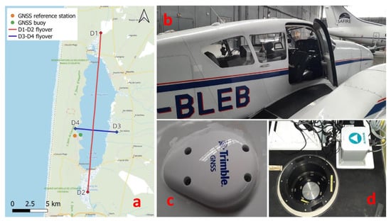
Figure 1.
(a) Map of Carcans-Hourtin Lake with locations of the buoy and reference station in relation to the two flight profiles. (b) Piper Aztec plane with direct GNSS antenna Trimble AV39 (c) on top of its fuselage. (d) Dedicated reflectometry antenna as seen from the aircraft cabin and iXblue inertial navigation system.
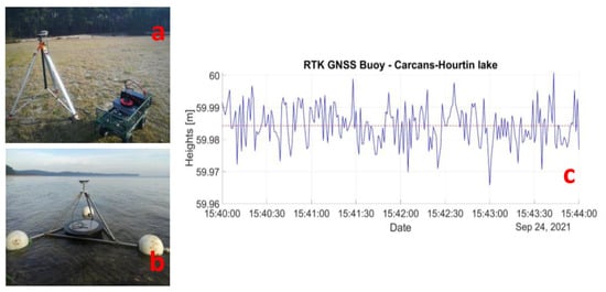
Figure 2.
(a) Reference station for RTK positioning of the in situ GNSS buoy (b). (c) Measurements of buoy heights obtained by RTK positioning when flying over D1–D2 profile. The mean value of the buoy height is represented by the red dotted line and is equal to 59.98 m.
2.2. On-Board Equipment
Emitted signals from GNSS satellites are electromagnetic waves with a right-handed circular polarization (RHCP), in which the electric field vector rotates in a right-hand motion with respect to the direction of propagation. When a reflection of the signal occurs on a surface at normal incidence, the ellipticity of polarization is preserved but the rotation direction is reversed. Once the incoming signal from GNSS satellites is reflected, the handedness of the polarized signal is reversed, especially for large elevation angles [8]. The antenna has therefore been developed to achieve optimum gain on the LHCP access. Characteristics of the reflectometry antenna were measured after its conception for validation. The maximum gain for the L1/E1 band is 7.2 dB and for the L5/E5 band 4.8 dB. The antenna also includes cross-polar isolation to avoid interferences between both RHCP and LHCP access. This antenna is positioned in the horizontal plane under the aircraft and is oriented towards the nadir to improve the reception of reflected signals (Figure 1). In addition, a Trimble AV39 GNSS antenna is installed on top of the plane to collect the direct signal and allows computation of its position, velocity, and time. Both antennas are connected to a high-frequency digitizer that enables a signal acquisition up to 205.824 MHz. Radio frequency (RF) signals collected by the antennas are first filtered and amplified before being digitalized. At last, an iXblue inertial navigation system is placed in the aircraft to serve as a reference and to measure the attitude of the aircraft. Measurements of pitch, roll and yaw are required to reposition the reflectometry antenna with respect to the direct one, enabling a lever arm correction to be calculated for altimetry determination.
2.3. Innovative Data Processing
Once digitized, RF signals are processed through three main steps. The first one is performed using a GNSS software receiver and consists of standard processing for the direct signal and open-loop correlation for the reflected one. The second step aims to filter the output of the software receiver and to extend the coherent integration time in order to increase the coherency of the signal. Finally, the last step is to estimate the heights of the reflection surfaces using a least-squares estimate after fixing the integer ambiguity values.
2.3.1. First Step: Dedicated Reflectometry Software
In order to process the raw reflected signal from GNSS satellites, the CNES developed a dedicated software receiver that includes a specific processing block for reflected signals. The dedicated receiver is a modified version of GNSS-SDR v0.0.15, an open-source GNSS software receiver developed by the Technological Center of Telecommunications of Catalunya (Spain) based on the signal processing development toolkit GNU Radio [9]. The initial structure of the software implements a classical direct signal processing block with parallel channels for each satellite. Each channel comprises an acquisition and a tracking block as well as a telemetry decoder block to read the navigation message. The tracking loops generate three code replicas named Early (E), Prompt (P) and Late (L), respectively, and two carrier replicas named In-phase (I) and Quadrature (Q), respectively, which are multiplied by the incoming signal to form six parallel correlation channels. Once the tracking loops are locked, the code Prompt replica and the carrier In-phase replica generated from the Numerical Commanded Oscillator (NCO) are successively multiplied with the incoming direct signal and integrated, allowing the computation of the correlation functions from which traditional pseudo-range and carrier phase measurements are derived. With a new block implemented in a master–slave configuration, Figure 3, open-loop processing using replicas of the carrier and code of the direct signal is performed for the reflected one. This allows us to mitigate tracking problems that may be related to low reflected signal amplitude [10]. The main difficulty in processing the reflected signal lies in determining the delay to be applied to the code replicas in order to carry out the correlation. This is why 3 replicas are generated for the direct signal, 1 with a maximum of 1 chip in advance, 1 synchronized with the received code and 1 with a maximum of 1 late chip. The processing block for reflected signal allows the user to choose a larger number of correlator delays, making the correlation function more precise. In the processing of Carcans-Hourtin Lake, the correlation of the reflected signal was performed with 21 delayed code replicas. After a short period of acquisition, the position, velocity, and time of the rover are calculated, and the software provides correlator outputs containing, for each satellite, the direct and reflected signal I and Q complex correlators with a coherent integration time of usually 1 or 4 ms, depending on the signal used.
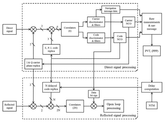
Figure 3.
Signal processing architecture of modified GNSS SDR for a reflectometry application. The same carrier and code replicas are used for direct and reflected processing.
2.3.2. Second Step: Prolongation of the Coherent Integration
Considering the simplest model with a plane reflection surface and satellite at an infinite distance as shown in Figure 4, the elongation of the reflected signal collected by the reflectometry antenna B with respect to the direct signal received by the direct antenna A is defined as follows [7]:
where h is the height between the aircraft and the reflection surface and is the elevation of satellite . In classic GNSS processing, the coherent integration time (CIT) for the C/A code is limited to the data message bit length (20 ms) due to sign changes that can prevent signal coherency. Thus, to improve the performance of carrier-phase altimetry and its range of use, the CIT can be increased. To do so, navigation data must be corrected for sign changes using an operation of data wipe-off expressed, for each correlator output i, as:
where sign[.] is the operator that returns the sign of the value between brackets. are the I and Q components of the direct and reflected signal of the ith correlator. is the Prompt correlator for component I of the direct signal. Direct and reflected complex outputs are then defined as:
where j is the complex number such that j2 = −1. The data sign is extracted from the direct In-phase and Prompt correlator channel and multiplied to the reflected correlators so as to remove the sign inversions. This operation is crucial for increasing the coherent integration time as shown in Figure 5. Once this has been carried out, we can extend the coherent integration while applying an apodization window to remove high-frequency noise. The Hamming window applied on samples is defined as:
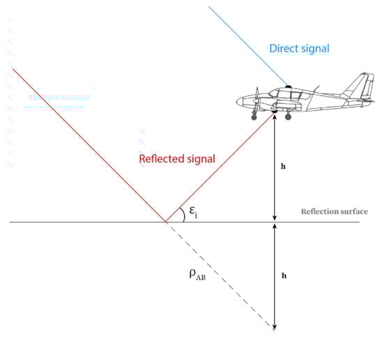
Figure 4.
Drawing of the reflection for an airborne reflectometry campaign. The model considered here is the simplest, with a plane reflection surface and satellite at an infinite distance with parallel rays.
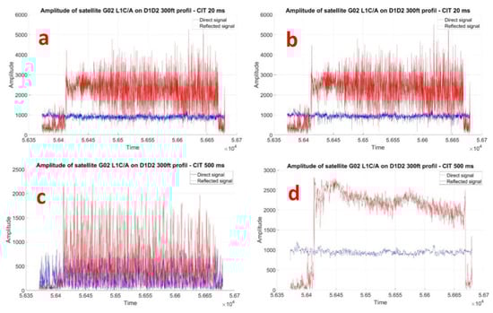
Figure 5.
Examples of graphs showing the effect of increasing the coherent integration time for the direct signal (solid blue line) and the reflected signal (solid red line). The amplitude of the reflected signal appears larger than the direct signal because the reception chain of the reflected channel had more gain than that of the direct channel. (a) Vector magnitude for a CIT of 20 ms without data wipe-off. (b) Vector magnitude for a CIT of 20 ms after data wipe-off. (c) Vector magnitude for a CIT of 500 ms without data wipe-off. (d) Vector magnitude for a CIT of 500 ms after data wipe-off. We can observe that a data wipe-off operation is required to extend coherent integration over 20 ms.
For the direct signal, we extend the coherent integration by applying the apodization window to each correlator output. The complex output of the ith correlator after extending the coherent integration over samples centered on the apodization window around time is defined as:
The resulting signal can again be broken down into a real and an imaginary part as follows:
The processing is the same for the reflected signal and the resulting signal can also be decomposed into a real and an imaginary part, thus giving:
Subsequently, decimation is applied to the data obtained from the previous equations to reduce calculation time while maintaining good accuracy of water level estimates. To obtain the maximum amplitude of the reflected signal, research for the correlator with the maximum power is performed. The same process is applied to the direct signal to check that the tracking was carried out under good conditions. In that case, the correlator with the maximum power is indeed the Prompt correlator and the residual phase is close to zero (absence of cycle slip). Amplitudes of each correlator are first computed, then for each time , the one with the maximum amplitude is selected. Once carried out on all the data, phase measurement is obtained from the following equation:
where unwrap is an operator that unwrapped the carrier phase by correcting cycle jumps of +/−0.5 cycle and atan2 is the two-argument arctangent allowing a correct and unambiguous value of the phase shift. The phase shift in radians between the reflected and direct signal used in the following section is then given by:
2.3.3. Third Step: Computation of Corrections, Residuals, and Integer Values for Ambiguities
The final step of the data processing consists of fixing ambiguities and estimating the heights of the reflection surface. For this purpose, the unwound phase is set between 0 and 1 phase cycles at the beginning of the profile in order to set the fractional part of the ambiguity, leaving the integer value to be determined. Considering the simplest model described in Figure 4, the elongation of satellite i, which corresponds to the phase shift expressed in carrier cycles, is related to the reflection surface height through the following equation:
where is the integer ambiguity value of the reflected signal for each satellite i, is the precise wavelength of the signal (i.e., approximately 19.03 cm for GPS L1 C/A signal), h is the height of the reflection surface, is the satellite elevation, b is the antenna bias between reflected and direct antenna and is introduced since both RF collecting chains are not exactly similar, is the correction of the lever arm required to correct the position of the reflection antenna related to the direct one and is the modeled correction for the additional delays induced by the troposphere.
Lever Arm Correction
In our calculation process, data from both antennas are compared. One problem is that the reflected and direct antennas are not positioned in the same place on the aircraft fuselage. So, in order to correct the lever arm, the positions of both antenna reference points were accurately measured with a laser tracker in the reference frame of the inertial unit. In the same reference frame, the phase centers of the antennas are considered to be constantly in the up direction. As the INS also provides parameters known as the attitude of the aircraft, which are pitch, roll and yaw measured in radians, it is possible to calculate a correction value for a given satellite of known elevation and azimuth.
Tropospheric Delay Correction
Another essential correction to compute is the tropospheric delay. When a GNSS signal crosses a layer of the troposphere, it is delayed depending on several parameters such as the angle of incidence and the state of the troposphere in terms of temperature, pressure and humidity. With reflectometry, the reflected signal passes through a thicker layer of troposphere than the direct signal, and an extra delay in the measurement must then be corrected. For a first approach, this delay can be expressed, from [11], as:
where n is the refractive index of air and is related to the refractivity N according to . In our case (Figure 6), the delay can then be expressed as:
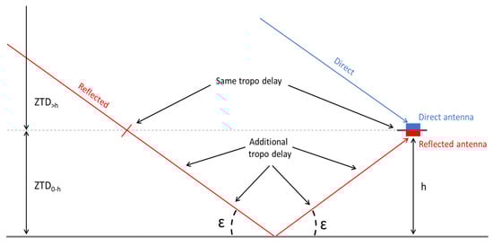
Figure 6.
Schematic illustration of tropospheric delay. As can be seen, the reflected signal passes through an additional layer of the troposphere, causing an additional delay in the propagation of the signal.
The refractivity can be divided into hydrostatic Nhydr (i.e., dry gases) and wet Nwet (i.e., water vapor) components such as . It can then be expressed as a function of air total pressure P [hPa], temperature T [K] and water vapor pressure e [hPa] as:
where , and are air refractivity coefficients estimated by both theory and experimentation [12,13]. Meteorological parameters are obtained from a global model of pressure and temperature called GPT [14]. The tropospheric delay of the additional travel incurred by the reflected signal can be described as:
Pseudo-Observation Computation to Fix Ambiguities
Equation (10) is given for each satellite i in view. Taking into account that reflections occur close enough to each other, we estimate an a priori waterline ellipsoidal height . This estimate can be, on a first approach, the height obtained from the GNSS buoy or any other way. An easier way to perform this estimation is to express this waterline height as a residual of an approximate value as follows:
According to this, the approximate height can be expressed as:
where is the plane height computed from the direct GNSS antenna using RTK or PPP methods. Equation (10) can then be expressed for each epoch as:
In addition to the height’s residuals and antenna bias which must be estimated, the last unknown parameter in Equation (17) is the integer ambiguity value . A first approach to fix these values is to estimate them from the measurements at the starting epoch (i.e., at which only the fractional part of the carrier phase is considered). Then, in the absence of carrier phase cycle slip, ambiguity remains constant throughout the pass and its value can be calculated to a first approximation using the following equation:
The right part of Equation (17) represents the pseudo-observations and is firstly computed using this estimated integer ambiguity value (Equation (18)). An examination of their graphical representation can then confirm whether or not the ambiguity values are already well defined. Indeed, we expect the pseudo-observations to be ordered in ascending order of the elevation of each satellite. In the opposite case, there is a need to fix the integer ambiguities values. To do so, we simply add or subtract one or several integers to the estimated ambiguity value for the non-ordered pseudo-observations. Once written for all the satellites with the fixed ambiguities, Equation (17) forms an overdetermined linear system Ax = B, whose unknowns and are determined by least-squares. There are two methods of resolution, either by estimating the surface height and the instrumental bias epoch by epoch or by assuming that the bias is constant during the flyover so that a single value is estimated. The second approach is a little more demanding in terms of computing resources. The least-squares problem can be expressed as:
Method 1 (epoch by epoch):
Method 2 (constant bias):
A full example of this resolution strategy on experimental data of Carcans-Hourtin is described in detail in the next section.
3. Results
This section presents an example of processing realized on Carcans-Hourtin data. Transverse flyovers were performed over the lake, the lengthwise profile is referenced as “D1–D2” and the widthwise profile is referenced as “D3–D4”.
3.1. Data Processing
Firstly, the data were processed in the dedicated software with an initial integration time of 1 ms. All complex correlator outputs were then post-processed in order to extend the coherent integration time as mentioned in Section 2.3.2. Prolongation of the coherent integration time and filtering with a hamming window allows us to greatly increase the coherency of the signal and to reduce the high-frequency carrier phase noise. Figure 7 shows the effect of extending the coherent integration time from 1 ms up to 500 ms. As we can observe, this operation greatly improves the coherency of the signal which can be estimated by watching the roundness of the phase shift on the phasor diagram. Once the complex correlators had been filtered, research for the correlator with the maximum amplitude was performed. For a direct signal, the Prompt correlator was always the one with the maximum amplitude as expected. However, for the reflected signal, several correlators had a high amplitude around the 10th correlator and the application of this algorithm maximized the resulting signal amplitude. To perform the computation of the lever arm correction and tropospheric delay correction (Figure 8), the measurements from the direct GNSS antenna were processed as well as those of the buoy and the inertial unit. A key point in the processing is then to time-shift all these data accurately. To do this, we need to check that the unwrapped phase is consistent with the aircraft’s altitude. When all the data matches (Figure 9), the next step is to fix integer ambiguity values in order to estimate the heights of the reflection surface.
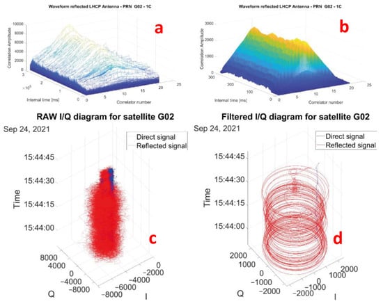
Figure 7.
(a) The 21 correlator outputs of raw reflected signal over time. (b) All the complex correlators were filtered with a prolongation of coherent integration over 500 ms as described in Section 2.3.2. It can be seen that the maximum correlator is around the 10th correlator. (c) Phasor diagram of the strongest raw correlator output for the reflected signal of satellite G02 over time. (d) The signal was filtered with a prolongation of coherent integration over 500 ms as described in Section 2.3.2. The loss of amplitude at the end of the flyover is consistent with the transition period between water and land.
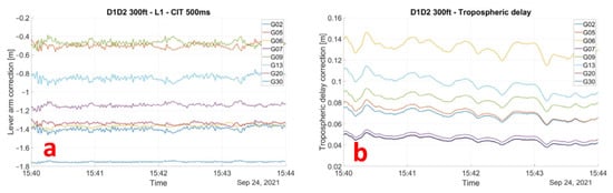
Figure 8.
(a) Lever arm correction computed along the D1–D2 profile using the inertial unit data and the relative position of both antennas. (b) Tropospheric delay corrections along the D1–D2 profile as described in Section 2.3.3. The tropospheric delays are consistent with GNSS satellite elevation and aircraft altitude.
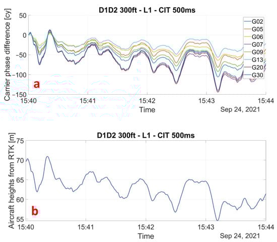
Figure 9.
(a) Unwrapped phase for each satellite in view during D1–D2 flyover. (b) Aircraft heights for D1–D2 flyover obtained from GNSS RTK positioning. The unwrapped phases are consistent with the aircraft height which is what we expect since the elongation of the reflected path depends on ĥ from Equation (1).
3.2. Ambiguity Resolution
Before performing an ambiguity resolution on data, the pseudo-observation residuals from the right-hand side of Equation (19) must be computed using the estimated integer ambiguity from Equation (20). Figure 10a shows that the pseudo-observations of satellite G06 are not consistently ordered with the other satellites and with the satellite elevation. This means that the integer ambiguity at the beginning of the profile is not correctly determined and that there is a need to correct them. We can manually fix the integer ambiguity by adding 1 to the estimated value. As shown in Figure 10b, the method makes it possible to correct the initial ambiguities, as demonstrated by the fact that the pseudo-observations are all consistent with each other. Moreover, the pseudo-observations cross at the moment when the aircraft is closest to the buoy, which is expected since the initial value from the buoy is taken as a reference.
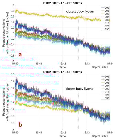
Figure 10.
(a) Residuals measurement for flyover D1–D2, with aircraft altitude of approximately 300 feet. The residuals are computed from the right-hand side of Equation (19) using the ambiguity integer values estimation from Equation (20). (b) This time, ambiguities were fixed by subtracting 1 from the estimated ambiguity value of satellite G06, the residuals are now consistent with the satellite elevation (G06 is the satellite with the lowest elevation).
3.3. Reflection Surface Height Computation
Now that integer ambiguity is fixed, we can proceed to the least-squares estimation of the surface reflection height residuals and the antenna bias between reflected and direct antenna. The least-squares estimate of can then be added to the initial value of to compute the reflection surface altitude as described in (17). Figure 11 shows the estimated heights of the reflection surface for the D1–D2 flyover using the L1 C/A signal of GPS satellites with a constant antenna bias estimated to be , and the estimated heights of the reflection surface for the D3–D4 flyover with a constant antenna bias of . As we can see for the D1–D2 flyover, the estimated values are consistent with the buoy measurement with a difference of 3.6 mm, as well as with the D3–D4 estimation at the intersection with a difference of 7.8 mm. Buoy and cross-profile heights were obtained by taking the mean value of a 2 s window around the time when the aircraft is closest to these points. The geoid slope deduced from the estimated heights, after converting the flight duration in distance with respect to the speed of the aircraft (Figure 12) is 7.1 mm/km. In comparison, the French altimetric conversion surface RAF20, which can be considered a local geoid model, gives a slope of 8.4 mm/km on the same D1–D2 profile. The height of the lake surface estimated from the measurements of profile D3–D4 is consistent with those of profile D1–D2, with a difference in height at their intersection of 3.3 mm. However, the difference in height with the buoy (20.9 mm) is significantly greater. The values of height and geoid slope differences obtained with different observations from the compared observations are summarized in Table 1.
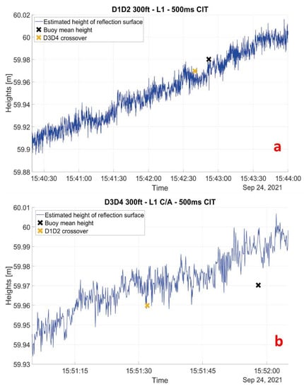
Figure 11.
(a) Least-squares estimated reflection surface heights along flyover D1–D2. The black cross represents the mean buoy height and is timed when the aircraft is closest to the buoy. (b) Least-squares estimated reflection surface heights along flyover D3–D4. The black cross represents the mean buoy height and is timed when the aircraft is closest to the buoy. The orange cross represents the value of each cross flyover at the intersection.
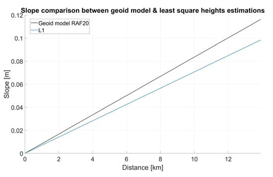
Figure 12.
Slope comparison of the height values obtained from least-squares estimation for signal GPS L1 C/A, and a local altimetric conversion surface RAF20. The slopes for the estimated values are 7 mm/km and 8.4 mm/km for RAF20.

Table 1.
Difference between observed values for the two profiles above Carcans-Hourtin Lake with an aircraft at 300, 500, 1000 and 2000 ft. Values in the table are discrepancies between the comparative method and the reflectometry estimate. Buoy and cross-profile discrepancies are calculated using a 2 s window around the closest point to the aircraft.
The same calculations were carried out on other signals such as GPS L5, Galileo E1 and E5, always with measurements acquired at an altitude of 300 feet. All the estimated heights are shown in Figure 13. As we can observe, estimated heights from L1, E1 and E5 are highly consistent between themselves. Heights computed from L5 are shifted, but it should be noted that only two satellites broadcasting this signal were in sight at the time of the flyover. As the altitude of the aircraft increases, we might expect more corrections to be needed, such as geodetic correction to compensate for the simplicity of the model used in the first place for the calculation (i.e., the flat reflection surface and the infinite distance between the satellites). Simulations using a model of the Earth’s surface in which reflection occurs on an ellipsoid to include the Earth’s surface curvature showed that for satellites with elevations greater than 20°, the elongation is less than 1 cycle (Figure 14) and is therefore not significant in the first instance for ambiguity determination. However, including a correction of the optical path difference with a more complex model can improve the accuracy of the resolution method, especially for high antennas. We computed the estimated height of the reflection surface for altitudes of 500, 1000 and 2000 feet. The results are shown in Figure 15 and compared values are summarized in Table 1. The estimated heights are consistent from one flyover to another, as well as with the buoy measurement. Flights at 300 ft and 1000 ft give very similar values of estimated heights. At 500 ft, heights obtained between 15:59:30 UTC and 16:01:30 UTC are not consistent with the geoid slope, as with the profile at 300 ft, but it can be observed on the buoy measurements that the lake surface height is decreasing during this flyover. On the 2000 ft profile, we can observe a slight stall around 16:39:35 UTC, not visible on the buoy measurement, which may be related to an error in the RTK aircraft trajectory. Further investigations are being performed to understand its origin.
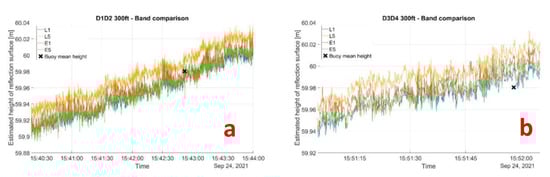
Figure 13.
(a) Estimated heights for D1–D2 flyover at 300 ft using GPS signals L1 and L5, and GALILEO signals E1 and E5. Heights computed from L1, E1 and E5 are highly consistent with each other and with the buoy measurements with less than 1 cm of error. Values estimated from L5 are shifted, but the estimation is performed using the only two satellites in sight. (b) Estimated heights for the D3–D4 flyover. Values are still consistent between L1, E1 and E5 and the buoy measurement is approximately 1 cm less.
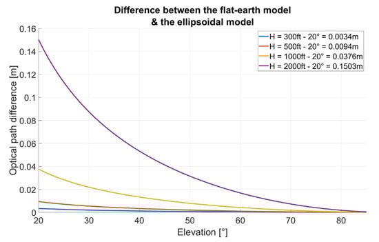
Figure 14.
Simulations of the optical path difference between a reflection on a flat earth model and an ellipsoidal model. For a 2000 ft flight with a satellite at 20° of elevation, the optical path difference is 0.1503 m.
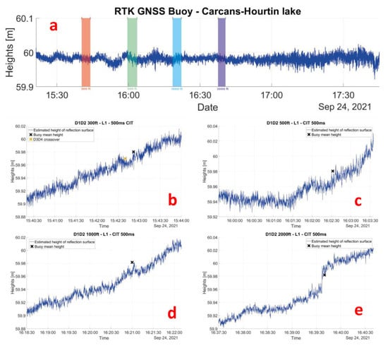
Figure 15.
(a) GNSS buoy measurements of the reflection surface heights from RTK positioning. Colored areas represent the aircraft’s flyover times at different altitudes. (b) Estimated heights for D1–D2 flyover and L1 signal at 300 ft. Buoy measurement and D3–D4 flyover measurement are, respectively, represented by the black and orange cross. (c) Estimated heights for D1–D2 flyover and L1 signal at 500 ft. The beginning of the profile match with a height variation observed on the buoy measurement. (d) Estimated heights for D1–D2 flyover and L1 signal at 1000 ft. Values are highly consistent with the 300 ft estimated values. (e) Estimated heights for D1–D2 flyover and L1 signal at 2000 ft. Even if the values are consistent with other profiles, an unidentified stall can be observed around 16:39:35.
4. Discussion
It is important to note that the aircraft position, obtained from a GNSS kinematic determination, needs to be sufficiently accurate to be used in the process. Implementation of more precise positioning methods for the aircraft can increase the precision and reliability of the reflection surface height estimations. Moreover, an approximation of the reflection surface height is needed for use as an initial value during the computation of residuals. Other processing techniques are being studied in order to quantify the impact of these initial guesses on the least-squares estimation of the reflection surface heights. At last, the integer ambiguity fixing method is easily implemented and shows good results, but it is currently carried out by hand. The implementation of a more automatic and efficient resolution is being studied using the LAMBDA method from Teunissen [15]. Other areas for improvement are also being studied, such as taking into account variations in the antenna phase center, or using more advanced models to calculate tropospheric delay correction.
5. Conclusions
Processing of the carrier phase shift used in this experimentation gives satisfactory results on the reflection surface height retrieval. At 300 ft, the deviation between the buoy and estimated values is less than 1 cm of error for the D1–D2 flyover with L1, E1 and E5 signals, and the slope of the estimated values is highly consistent with the slope of the local geoid RAF20. For D3–D4, even if the slope is still consistent with the local geoid, estimated heights are less close to the buoy values, with more than 2 cm of error. By increasing the initial altitude of the aircraft, we observe a good redundancy on the estimated surface height values and coherency with the buoy measurements. However, unidentified events are still being studied, especially for higher altitudes, and there might be a need to include geodetic corrections.
Author Contributions
Conceptualization, N.V., J.V., J.C. and L.L.; methodology, V.N, J.V., J.C and L.L.; software, N.V.; validation, N.V.; formal analysis, J.V., J.C. and L.L.; writing—original draft, N.V.; writing—review & editing, J.V., J.C. and L.L.; supervision, J.V.; funding acquisition, J.V. All authors have read and agreed to the published version of the manuscript.
Funding
This research received no external funding.
Conflicts of Interest
The authors declare no conflict of interest.
References
- Hall, R.C.C. Multistatic scatterometry. In Proceedings of the IEEE International Geoscience and Remote Sensing Symposium, Edinburgh, UK, 12–16 September 1988. [Google Scholar]
- Larson, K.M.; Small, E.E.; Gutmann, E.D.; Bilich, A.L.; Braun, J.J.; Zavorotny, V.U. Use of GPS receivers as a soil moisture network for water cycle studies. Geophys. Res. Lett. 2008, 35, L24405. [Google Scholar] [CrossRef]
- Rodriguez-Alvarez, N.; Bosch-Lluis, X.; Camps, A.; Vall-Llossera, M.; Valencia, E.; Marchan-Hernandez, J.F.; Ramos-Perez, I. Soil Moisture Retrieval Using GNSS-R Techniques: Experimental Results Over a Bare Soil Field. IEEE Trans. Geosci. Remote Sens. 2009, 47, 3616–3624. [Google Scholar] [CrossRef]
- Munoz-Martin, J.F.; Perez, A.; Camps, A.; Ribó, S.; Cardellach, E.; Stroeve, J.; Nandan, V.; Itkin, P.; Tonboe, R.; Hendricks, S.; et al. Snow and Ice Thickness Retrievals Using GNSS-R: Preliminary Results of the MOSAiC Experiment. Remote Sens. 2020, 12, 4038. [Google Scholar] [CrossRef]
- Larson, K.M.; Löfgren, J.S.; Haas, R. Coastal Sea level measurements using a single geodetic GPS receiver. Adv. Space Res. 2013, 51, 1301–1310. [Google Scholar] [CrossRef]
- Roussel, N.; Ramillien, G.; Frappart, F.; Darrozes, J.; Gay, A.; Biancale, R.; Striebig, N.; Hanquiez, V.; Bertin, X.; Allain, D. Sea level monitoring and sea state estimate using a single geodetic receiver. Remote Sens. Environ. 2015, 171, 261–277. [Google Scholar] [CrossRef]
- Lestarquit, L.; Peyrezabes, M.; Darrozes, J.; Motte, E.; Roussel, N.; Wautelet, G.; Frappart, F.; Ramillien, G.; Biancale, R.; Zribi, M. Reflectometry With an Open-Source Software GNSS Receiver: Use Case With Carrier Phase Altimetry. IEEE J. Sel. Top. Appl. Earth Obs. Remote Sens. 2016, 9, 4843–4853. [Google Scholar] [CrossRef]
- Born, M.; Wolf, E.; Bhatia, A.B.; Clemmow, P.C.; Gabor, D.; Stokes, A.R.; Taylor, A.M.; Wayman, P.A.; Wilcock, W.L. Principles of Optics: Electromagnetic Theory of Propagation, Interference and Diffraction of Light, 7th ed.; Cambridge University Press: Cambridge, UK, 1999. [Google Scholar] [CrossRef]
- Fernandez-Prades, C.; Arribas, J.; Closas, P.; Aviles, C.; Esteve, L. GNSS-SDR: An Open-Source Tool for Researchers and Developers. In Proceedings of the 24th International Technical Meeting of the Satellite Division of The Institute of Navigation (ION GNSS 2011), Portland, OR, USA, 19–23 September 2011; pp. 780–794. [Google Scholar]
- Löfgren, J.S.; Haas, R. Sea level measurements using multi-frequency GPS and GLONASS observations. EURASIP J. Adv. Signal Process. 2014, 2014, 50. [Google Scholar] [CrossRef]
- Saastamoinen, J. Atmospheric correction for the troposphere and stratosphere in radio ranging of satellites. In Geophysical Monograph Series; Henriksen, S.W., Mancini, A., Chovitz, B.H., Eds.; American Geophysical Union: Washington, DC, USA, 2013; pp. 247–251. [Google Scholar] [CrossRef]
- Smith, E.K.; Weintraub, S. The Constants in the Equation for Atmospheric Refractive Index at Radio Frequencies. Proc. IRE 1953, 41, 1035–1037. [Google Scholar] [CrossRef]
- Thayer, G.D. An improved equation for the radio refractive index of air. Radio Sci. 1974, 9, 803–807. [Google Scholar] [CrossRef]
- JBoehm, J.; Heinkelmann, R.; Schuh, H. Short Note: A global model of pressure and temperature for geodetic applications. J. Geod. 2007, 81, 679–683. [Google Scholar] [CrossRef]
- Teunissen, P.J.G. Theory of carrier phase ambiguity resolution. Wuhan Univ. J. Nat. Sci. 2003, 8, 471–484. [Google Scholar] [CrossRef]
Disclaimer/Publisher’s Note: The statements, opinions and data contained in all publications are solely those of the individual author(s) and contributor(s) and not of MDPI and/or the editor(s). MDPI and/or the editor(s) disclaim responsibility for any injury to people or property resulting from any ideas, methods, instructions or products referred to in the content. |
© 2023 by the authors. Licensee MDPI, Basel, Switzerland. This article is an open access article distributed under the terms and conditions of the Creative Commons Attribution (CC BY) license (https://creativecommons.org/licenses/by/4.0/).