The Seasonal Variations Analysis of Permanent GNSS Station Time Series in the Central-East of Europe

Abstract

Observations from permanent GNSS stations are actively used for the research and monitoring of geodynamic processes. Today, with the use of modern scientific programs and IGS products, it is possible to determine GNSS station coordinates and velocities at the level of a few millimeters. However, the scientific community constantly faces the question of increasing the accuracy of coordinate definitions to obtain more reliable data in the study of geodynamic phenomena. One of the main sources of errors is systematic measurement errors. To date, the procedure for their removal is still incomplete and imperfect. Also, during the processing of long-term GNSS measurements, it was found that the coordinate time series, after the removal of trend effects, are also characterized by seasonal variations, mainly of annual and semi-annual periods. We estimated the daily coordinate time series of 10 permanent GNSS stations in the central-eastern part of Europe from 2001 to 2019 and calculated the seasonal variation coefficients for these stations. The average value of the coefficients for the annual cycle for the N, E, and H components is −0.7, −0.2, and −0.7 mm, and for the semi-annual cycle the average value is 0.3, 0.4, and −0.5 mm. The obtained coefficients are less than 1 mm, which is why it can be argued that there is no seasonal component in the coordinate time series or that it is so small that it is a problematic task to calculate it. This practical absence of a seasonal component in long-term time series of GNSS coordinates, in our opinion, is partly compensated by the use of modern models of mapping functions (such as VMF3) for zenith tropospheric delays instead of the empirical GMF. To test the obtained results, we calculated the coefficients of seasonal variations for the sub-network of GNSS stations included in the category of the best EPN stations—C0 and C1. The values of the coefficients for the stations of this network are also less than 1 mm, which confirms the previous statement about the absence of a seasonal component in the long-term time series of coordinates. We also checked the presence of seasonal changes in the time series using the well-known decomposition procedure, which showed that the seasonal component is not observed because the content does not exceed 10% for additive decomposition and 20% for multiplicative decomposition.

1. Introduction

Today, coordinate time series of reference GNSS stations are widely used in different areas of geodetic and geophysical research, including the study of geodynamic processes [1,2,3,4,5,6]. The accuracy of determining the absolute coordinates of GNSS observation stations is at the level of 1 cm, and velocities are at the level of 1–2 mm/year. However, for studying more “subtle” geodynamic processes, it will very soon be necessary to increase the accuracy of coordinate determinations by an order of magnitude (at the level of 1 mm for coordinates and 0.1 mm/year for velocities). From the technical side, modern GNSS methods formally allow for the specified accuracy indicators to be approached. The biggest problem is considering the complex influence of the environment on the measurement results [7,8]. For this purpose, it is necessary to consider the Earth (including the “solid” shell, the ocean, and the atmosphere) as a whole to take into account with sufficient accuracy the effects influencing the state of the Earth’s surface at the location of the observation station. A significant number of geodynamic processes are currently quite well studied qualitatively, and their quantitative influence on the coordinates and gravitational field of the Earth can be considered at a certain level of accuracy. The residual estimates of the obtained coordinate time series should obey the ordinary Gaussian distribution law. This means that the influence of unextracted, correlated, systematic errors in the results of observations is minimized. However, in the practice of statistical analysis of large datasets, it is known that when parameter estimates are from the general population of individual values of a random variable, which is subject to the ordinary distribution law, then this is not a guarantee that the estimates themselves also have a normal distribution. In [9], it was established that the normality hypothesis is practically and theoretically untenable since the measurement errors do not obey the Gauss law but instead obey the type VII Pearson distribution with a diagonal Fisher information matrix. Based on the non-classical theory of measurement errors, the results obtained in [9] indicate that the procedure for removing systematic errors from measurement results is still incomplete and imperfect.

During the processing of long-term GNSS measurements, it was found that the coordinate time series, after the removal of trend effects, are also characterized by seasonal variations, mainly of annual and semi-annual periods. According to most scientists [10,11,12,13,14], such variations were caused by the influence of the atmosphere and hydrological loads. The amplitudes of such seasonal variations are several millimeters. Determining seasonal variations in the positions of GNSS observation points is important for understanding the natural processes that cause them.

However, such a behavior model of coordinate time series, consisting of linear velocity plus annual and semi-annual signals, can describe only a part of geophysical processes. The remaining signals in the GNSS time series, mainly with pseudo-periodic signals, can cause bias in the estimation of real periodic seasonal fluctuations. In the literature on this issue, “other” geophysical signals are divided into three groups. The first group includes signals caused by gravitational excitation (movement through the solid Earth, oceanic and atmospheric tides). Polar tides with a predominantly annual spectrum and Chandler wobble are also included in this group. In most cases, they can be modeled with millimeter accuracy (solid Earth tide model IERS2010, ocean tide models GOT00.2 and FES2004, or newer models such as TPXO9 and FES2014b) [15]. They are often used in conjunction with an elastic Earth model to simulate the corresponding load deformations. In most software packages used to process static GNSS observations, load deformations of both the solid surface of the Earth and the ocean are implemented [16,17]. Therefore, they should not appear in the time series if there are no errors in the ocean tide models near the studied stations.

The second group of such processes has a thermal origin (the effects of hydrodynamics or climate change). For example, fluctuations in surface pressure lead to fluctuations in sea level (without tides), groundwater, snow, and ice. All these signals cause a surface load that deforms the solid Earth in a similar manner to a load of ocean tides [3]. Atmospheric pressure loading (APL) impacts the annual period the most. In addition, seasonal variations can also occur due to Non-Tidal Ocean Loading (NTOL) in places where fluctuations in sea level and/or ocean bottom pressure are critical, such as near the coast. Among the existing software that estimates surface loading at each station, QOCA (QLM loading maps) can be noted. Surface load maps are also provided by the Global Geophysical Fluid Centre (GGFC) [18].

The third group of geophysical signals rearranges spurious signals and other residual errors that cause pseudoperiodic variations [19]. In general, these are transient signals of nonlinear characteristics associated with the nature of the Earth’s crust deformation on a local or regional scale after geophysical events. For example, post-seismic relaxations are usually modeled as logarithmic or exponential functions in the GNSS time series. It is often difficult to find post-seismic deformation when the duration of the transient response is limited in time or has a small amplitude. Another important type of signal is discontinuities, which can affect the estimation of other parameters (such as velocity and the stochastic model) if not correctly included in the analysis [20]. These discontinuities are usually caused by station-specific equipment changes or by a coherent spatial response to geophysical phenomena such as earthquakes, ionospheric disturbances, etc. Studies of the origin of discontinuity have shown that only parts of the discontinuity can be attributed to geophysical events or the metrological situation of the station. Residual offsets are most likely due to unrecorded station changes or sampled GNSS models and processing parameters, and the best method for detecting offsets remains a visual examination of the time series.

As part of the study of the earth’s crust movements, seasonal variations are usually considered as “noise”, an error that affects the determination of annual changes in the coordinates of GNSS stations [21,22]. The inclusion of annual and semi-annual signals in the process of evaluating coordinate changes is only one of the possible options. To reduce the impact of seasonal variations, approaches that considered a priori information about the parameters (coefficients) of such variations were proposed. At the same time, it was believed that the parameters of seasonal variations should practically coincide for collocated sites due to the common factors that cause them, and their determination was carried out using the least squares method. Further studies have shown that the total geophysical signals are far from ideal sine or cosine signals and contain a significant part of the random character. As a result, only seasonal signals with a constant amplitude can be obtained [21,23], which does not correspond to real seasonal fluctuations in which a time-varying amplitude of fluctuations is detected.

In recent years, published works [19,24,25] show that a harmonic model with time-varying amplitude can better model the seasonal variation. In the studies of various authors, it was proposed that seasonal signals could be isolated through methods such as wavelet decomposition (WD) [26], singular spectral analysis (SSA) [27,28], Weighted Nuclear Norm Minimization (WNNM) [29], etc. The results show that these methods have achieved promising results, although most have several limitations [30]. First, it is difficult to fully isolate these signals because their stochastic properties are usually correlated with colored noise in the GNSS time series [31]. It would be more appropriate to minimize these signals by eliminating the causes of their occurrence.

Therefore, high-precision processing of GNSS data is crucial for quantifying and interpreting geodynamic processes. However, strategies for such processing are complex and involve many assumptions and multivariate parameter selection [30]. In addition, some of the geophysical signals show similar temporal and spatial patterns, which requires additional analysis at the post-processing stage to decompose the time series into its constituent parts (decomposition) [32].

The main objectives and results of our study include the interpretation of discrepancies in the context of the individual accuracy of time series, which has been greatly improved by newer data processing methods, such as the estimation of percentage values of seasonal processes in cleaned time series and the simulation of a seasonal signal with constant amplitude and phase in long time series of GNSS coordinates.

Section 2 outlines the strategy for processing GNSS data using the GAMIT/GLOBK software package and describes the procedure for obtaining coordinate time series of EPN stations according to various criteria. The research results are analyzed in Section 3, where the limitations of modeling the seasonal signal with constant amplitude and phase in long GNSS time series and minimization in the residual time series of this signal after the procedure of their decomposition are emphasized.

2. Materials and Methods

The GNSS data selected for analysis in this paper were from the stations of the EUREF Permanent Network (EPN). The period of the data is from January 2001 to December 2019. To process GNSS data, we used the latest version of the GAMIT/GLOBK software developed by the Massachusetts Institute of Technology and the Scripps Institute of Oceanography [16]. GAMIT is based on the weighted least squares (double-difference) algorithm. Compared with the non-difference model, it can exclude the influence of satellite and receiver clock errors and reduce atmospheric refraction and orbit errors. GLOBK uses a Kalman filter whose input information includes estimated station coordinates, Earth rotation parameters, orbit parameters, and the covariance matrix calculated by GAMIT. A Kalman filter then combines the GAMIT solution in space and time. Finally, a reference frame is set to obtain information about the station coordinates, satellite orbit, Earth rotation, and other parameters in this frame.

The general scheme of standard GNSS observation processing in the GAMIT/GLOBK software package is presented in Figure 1.

For research, we selected 10 GNSS stations with a 19-year observation period (1094-2085 GPS weeks) operating in the EPN network. The location of 10 GNSS stations in Central-Eastern Europe is shown in Figure 2.

The selected GNSS data include 19 years of continuous observations, with an average amount of missing data of less than 3%. To minimize the influence of mounting the GNSS receiver antenna, the stations were chosen based on the principle of their installation on a stable foundation or within a low-rise building. Based on the low amount of missing data and 19 years of monitoring records, we consider the GNSS dataset to be a stable experimental environment.

Table 1. Modeling the observations in GAMIT/GLOBK software.

Satellite Orbit	IGS Tabulated Ephemeris
The motion of the Earth in inertial space	Analytical models for precession and nutation (tabulated); IERS observed values for pole position (wobble) and axial rotation (UT1) Solid Earth tide analytical model (IERS2010) Ocean and atmospheric tidal loading model (FES2004) Solar radiation pressure parameters model (Berne)
Propagation of the signal	Zenith hydrostatic (dry) delay (ZHD) from the ECMWF meteorological model through the VMF3 grids Zenith wet delay (ZWD) and ZHD mapped to line-of-sight with mapping functions (VMF3 grid) Variations in the phase centers of the ground and satellite antennas (ANTEX file)

shows the models and products that were used during the processing of GNSS measurements.

The first step of GAMIT/GLOBK processing is data collection and archiving. Orbits are downloaded automatically on a certain day during the processing in GAMIT/GLOBK. RINEX files for IGS/EPN stations can also be downloaded and unzipped automatically during processing if they are specified using entries in a control file. Local RINEX files can be manually added for processing by copying them into the domestic/RINEX directory.

The second step of GAMIT/GLOBK processing is raw (RINEX) data processing (GAMIT). GAMIT consists of several modules: makexp and makex to prepare the data for processing, arc and yawtab to generate reference orbit and rotation values for satellites, grdtab to interpolate time and specific location values of atmospheric and loading models, model to compute residual observations and partial derivatives from a geometrical model, autcln to detect outliers or break points in the data, and solve to perform least squares analysis [16]. GAMIT has two levels of accuracy assessment. The first level checks whether there are enough data to make a reasonable estimate, and the second level checks whether the model data meet the noise level. The primary indicator for the first criteria is the magnitude of the uncertainties of the baseline components, which should not be larger than the a priori constraints previously given by station coordinates and orbital parameters. The main indicator at the second level is nrms (normalized rms), the square root of chi-square per degree of freedom. Nrms is close to unity if the data are randomly distributed and the a priori weights are correct. In practice, with the default weighting scheme adopted in GAMIT to account for temporal correlations, a good solution usually has an nrms value of about 0.2. Anything larger than ~0.5 is removed from processing. If the final solution meets these two criteria, it can be used for further processing in GLOBK.

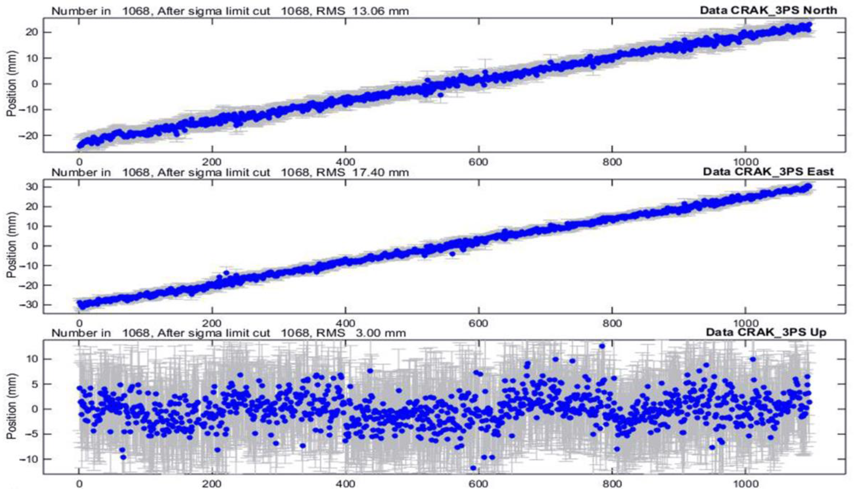
The third step in GAMIT/GLOBK processing is the generation of time series and velocities (GLOBK). GLOBK works with a specific program and its main function is to combine quasi-observations from GAMIT or those provided in SINEX format from multiple networks or epochs (glred or globk) and to apply a reference frame (glorg) to this solution. Globk and glred are the same program but called in different modes. Glred reads data one day at a time to generate a time series, while globk stacks multiple epochs to acquire the mean position or velocity. Final control over the data and processing of time series generated by glred is held in GLOBK. Uncertainties and reproducibility in the range of 1–2 mm in horizontal coordinates and 3–5 mm in height is achieved with 24 h sessions and robust stabilization. Glorg iterates the stabilization and removes sites with large elevation uncertainty or horizontal/elevation residuals compared to the uncertainty. In the last iteration, at least three sites should be left in stabilization and the RMS should be at the expected level of uncertainty (1–5 mm). A graphical representation of the coordinate time series of station CRAK estimated in GLOBK is presented in Figure 3.

Estimated coordinate time series can be used for the next purpose if the distribution of scatters is approximately Gaussian with a median nrms ~1.0. In our case, nrms = 0.29, so the generated coordinate time series could be used for our next stage of research.

3. Results

3.1. Modeling the Seasonal Signal with Constant Amplitude in Long GNSS Time Series

The coordinates generated in ITRF2014 were used as input for our analyses. The long-term daily processing data of an entire network (Figure 2) between 2001 and 2019 (1094-2085 GPS weeks) were used for the detection and determination of annual and semi-annual periodical changes in the stations’ NEU components. The individual component (north, east, or up) of the GNSS time series can be described as follows:

$$\left(t_i\right)=a+b{t}_i+ccos\left(2\pi \times t_i\right)+ds\left(2\pi \times t_i\right)+ecos\left(4\pi \times t_i\right)+fsin\left(4\pi \times t_i\right)+\epsilon \times t_i$$

(1)

$y$—N, E, and U components at $i$ epoch;

$a$—initial value;

$b{t}_i$—the linear trend (velocity);

$c$ i $d$—amplitudes of annual seasonal variations in station coordinates;

$e$ i $f$—amplitudes semi-annual seasonal variations in station coordinates;

$\epsilon \times t_i$—residuals (a measure of accuracy).

As a result of applying this equation, we will only receive seasonal signals with a constant amplitude [24], which may not correspond to real seasonal fluctuations.

Table 2. Coefficients of seasonal variations.

	N				E				H
Mm	c	d	e	f	c	D	e	f	c	d	e	f
CRAO	0.1	−0.2	0.1	0.1	−1.1	2.0	0.6	0.3	2.4	1.7	−0.4	−0.2
GANP	−0.3	−0.5	0.5	0.0	−0.3	−0.3	0.3	0.3	7.0	2.8	3.2	1.7
GLSV	−2.2	−0.1	0.4	0.2	−0.3	0.6	0.3	0.4	−1.2	−2.5	−0.3	−1.0
JOZ2	−0.2	0.3	0.0	0.4	−0.6	0.1	0.2	0.6	0.2	0.0	0.0	−0.4
KHAR	−2.7	−0.9	1.5	0.5	1.2	−0.2	0.3	0.6	−1.4	−2.7	0.5	−1.3
LAMA	0.0	−0.1	0.1	0.1	−0.2	0.0	0.0	0.1	−0.2	0.1	0.1	0.2
MIKL	0.0	0.1	0.0	0.1	−0.7	0.1	0.1	0.4	−0.1	0.0	0.0	0.0
POLV	−0.5	0.1	0.2	0.2	0.3	0.3	0.0	0.7	−0.6	−2.5	0.1	−1.5
SULP	−1.1	−0.7	−0.1	−0.2	−0.3	−0.4	−0.2	−0.1	−1.6	−3.3	−1.1	−2.7
UZHL	0.2	0.0	0.2	0.1	−0.4	−1.1	1.0	0.4	1.0	−0.8	0.6	0.3
Min	−2.7	−0.9	−0.1	−0.2	−1.1	−1.1	−0.2	−0.1	−1.6	−3.3	−1.1	−2.7
Max	0.2	0.3	1.5	0.5	1.2	2.0	1.0	0.7	7.0	2.8	3.2	1.7
mean	−0.7	−0.2	0.3	0.2	−0.2	0.1	0.3	0.4	0.5	−0.7	0.3	−0.5

shows the amplitudes of annual and semi-annual seasonal variations in station coordinates.

For the N component, the average value of the coefficients for the annual cycle (c, d) is −0.7 mm, and for the semi-annual cycle (e, f) this value is 0.3 mm. For the E component, the average value of the coefficients for the annual cycle is −0.2 mm, and for the semi-annual cycle this value is 0.4 mm. For the H component, the average value of the coefficients for the annual cycle is −0.7 mm, and for the semi-annual cycle this value is −0.5 mm. The obtained coefficients are so small (average values are less than 1 mm) that it can be argued that there is no seasonal component in the coordinates time series, or that it is so small that it is a problematic task to calculate it. In our opinion, the practical absence of a seasonal component in the long-term time series of GNSS coordinates lies in its partial compensation due to the use of modern models of VMF3 mapping functions for zenith tropospheric delays instead of the empirical GMF. The coefficients in the VMF3 model are functions of variable atmospheric pressure derived from a meteorological model of global pressure and temperature (GPT2w) [33]. This model was obtained based on multi-year average monthly profiles of pressure, temperature, and humidity in the form of a global grid (grid) with average values of meteorological parameters and annual and semi-annual fluctuations. However, the dependence on external data it is processing and the assumption that the differences between GMF and GPT are small may have been why ZHD VMF3 and GPT2w were not used regularly in the process of generating GNSS coordinate series.

To verify the stated statement, we also calculated the coefficients of seasonal variations in the coordinate time series for a period of 3 years (2018–2020) for the stations of the EPN network, which were divided into two sub-networks. Stations of class C0–C1, which includes the most stable and reliable stations of the EPN network, were selected for the first sub-network. Class C6 stations, which the EPN classifies as unstable, were selected for the second sub-network.

GNSS observation processing from the sub-networks of permanent stations (Figure 4) was performed using the GAMIT/GLOBK software in the same way as the previous network (see Figure 2).

Table 3. Statistical results of seasonal variation coefficients from sub-network C0–C1 and sub-network C6.

	N				E				H
mm	c	d	e	f	c	d	e	f	c	d	e	f
sub-network C0−C1
min	−1.2	−1.5	−0.6	−0.7	−1.7	−1.5	−0.4	−2.6	−2.6	−3.5	−2.8	−4.1
max	2.1	1.5	1.1	1.0	2.6	1.3	0.8	0.6	6.7	2.4	2.0	1.8
mean	−0.2	0.1	0.0	0.1	−0.1	0.0	0.0	0.0	0.4	−0.6	0.0	−0.1
sub-network C6
min	−3.4	−3.6	−2.4	−3.0	−2.6	−14.4	−1.8	−2.7	−8.1	−3.8	−2.6	−2.5
max	4.4	8.3	0.6	0.7	5.2	1.0	2.8	3.5	6.7	3.8	8.1	4.0
mean	0.1	3.7	−0.5	−0.3	0.4	−5.2	0.5	0.5	0.6	−2.9	3.7	1.8

shows the results of statistical analysis of the obtained coefficients of seasonal variations from the C0–C1 and C6 sub-networks (Figure 4).

For the N component, the average value of the coefficients in sub-network C0–C1 and sub-network C6 for the annual cycle is −0.2 mm and 3.7 mm, respectively, while for the semi-annual cycle the average value is 0.1 mm and −0.5 mm, respectively. For E, the average value of the coefficients for the annual cycle is −0. 1 mm and−5. 1 mm, while for the semi-annual cycle the average value is 0.0 mm and 0.5 mm. For the H component, the average value of the coefficients for the annual cycle is −0.6 mm and −2.9 mm, while for semi-annual cycle the average value is −0.1 mm and 3.7 mm. The obtained average values of the coefficients of seasonal variations, as well as the coefficients obtained from the networks (see Table 2), are less than 1 mm. In sub-network C6, in contrast to the networks (Figure 2) and the C0–C1 sub-network, the average values of the coefficients of seasonal variations are larger (up to 5 mm). The unreliability of the stations may cause this. We noted that with increases in the time interval of observations, the coefficients of the seasonal variations of class C6 stations decreased.

To verify the obtained results, we also compared the calculated coefficients of seasonal variations from four class C1 permanent stations (BRUX, CRAK, POUS, WARE) using the GAMIT/GLOBK software with the corresponding coefficients of seasonal variations obtained from EPN solutions [34] based on Bernese GNSS Software.

Table 4. Statistical results of seasonal variations coefficients from sub-network C1 using GAMIT/GLOBK and Bernese.

Station	N				E				H
mm	∆c	∆d	∆e	∆f	∆c	∆d	∆e	∆f	∆c	∆d	∆e	∆f
BRUX	0.1	−0.2	0.1	−0.4	0.3	5.0	0.1	2.4	−0.2	0.3	−0.5	−0.1
CRAK	−0.3	−0.1	−0.1	−0.1	0.1	0.5	−0.1	−0.3	−0.1	−0.3	−0.4	−0.2
POUS	−0.3	−0.1	0.0	−0.3	0.2	1.1	−0.3	0.1	1.8	0.0	−0.2	−0.8
WARE	−0.1	0.1	0.1	−0.2	0.9	0.5	−0.1	−0.2	0.0	0.1	−0.3	−0.1
min	−0.3	−0.2	−0.1	−0.4	0.1	0.5	−0.3	−0.3	−0.2	−0.3	−0.5	−0.8
max	0.1	0.1	0.1	−0.1	0.9	5.0	0.1	2.4	1.8	0.3	−0.2	−0.1
mean	−0.2	−0.1	0.0	−0.2	0.4	1.8	−0.1	0.5	0.4	0.0	−0.3	−0.3

shows the results of the statistical analysis of seasonal variation coefficients from the C1 stations using GAMIT/GLOBK and Bernese software Version 5.2.

3.2. Decomposition of GNSS Time Series

The next step of our research was to investigate the presence of seasonal changes in the coordinate time series. Decomposition procedures are used in time series to describe trends (increase or decrease in value), seasonal factors (repeating short-term cycles), and noise (random variation). There are two forms of classical decomposition: an additive form and a multiplicative form. The time series is called additive if the time series components are added together to make the time series. Through visualization, a time series is categorized as additive if increasing or decreasing patterns in the time series are similar throughout the series. The mathematical function of any additive time series can be represented by

$$y_t=S_t{+T}_t+R_t$$

(2)

$$y_t=S_t{+T}_t+r_t+{\epsilon }_t$$

(3)

where $y_t$ represents the data, $S_t$ is the seasonal component, $T_t$ is the trend-cycle component, and $R_t$ is the remainder component, all at period $t$.

Time series are called multiplicative if all components of the time series are multiplied together. Through visualization, if the time series exhibits exponential growth or decrements with time, then such a time series can also be considered multiplicative. The mathematical function of multiplicative time series is

$$y_t=S_t{\ast T}_t\ast R_t$$

(4)

Identifying whether a series is additive or multiplicative is trickier than it might be suggested. Oftentimes, one component of the time series might be additive while the others are multiplicative. That is why we propose the use of both of these methods.

Also, for the approbation of the obtained results from additive or multiplicative methods, the RegARIMA model [35] was offered. With the help of this model, the input time series were decomposed into a linear deterministic component and a stochastic component. The deterministic part of the series can contain outliers and regression effects. The stochastic part is defined by a seasonal multiplicative ARIMA model. The RegARIMA model is specified as

$$z_t=y_t\beta +x_t$$

(5)

$z_t$ is the original series; $\beta =\left({\beta }_{1,\cdots ,}{\beta }_n\right)$ is a vector of regression coefficients; $y_t=\left(y_{1t,\cdots ,}{y}_{nt}\right)$ are n regression variables (outliers, user-defined variables); and $x_t$ is a disturbance that follows the general ARIMA process:

$$\mathsf{\varphi }\left(\mathrm{B}\right)\delta \left(B\right)x_t=\theta \left(B\right){\alpha }_t$$

(6)

where $\mathsf{\varphi }\left(\mathrm{B}\right),\delta \left(B\right)$, and $\theta \left(B\right)$ are finite polynomials in B (backshift operator) and ${\alpha }_t$ is a white noise variable with zero mean and a constant variance. The polynomial $\mathsf{\varphi }(\mathrm{B}$) is a stationary autoregressive polynomial in $B$, which is a product of the stationary regular autoregressive polynomial in $B$ and the stationary seasonal polynomial in ${\mathrm{B}}^{\mathrm{s}}$:

$$\mathsf{\varphi }\left(\mathrm{B}\right)={\mathsf{\varphi }}_{\mathrm{p}}\left(\mathrm{B}\right){\mathsf{\Phi }}_{\mathrm{b}\mathrm{p}}\left({\mathrm{B}}^{\mathrm{s}}\right)$$

(7)

where p is the number of regular AR terms, bp is the number of seasonal moving average terms, and s is the number of observations. The polynomial $\theta \left(B\right)$ is an invertible moving average polynomial in $B$, which is a product of the invertible regular moving average polynomial in $B$ and the invertible seasonal moving average polynomial in ${\mathrm{B}}^{\mathrm{s}}$:

$$\theta \left(B\right)={\theta }_q\left(B\right){\mathsf{\Theta }}_{\mathrm{b}\mathrm{q}}\left({\mathrm{B}}^{\mathrm{s}}\right)$$

(8)

The polynomial $\delta \left(B\right)$ is the non-stationary autoregressive polynomial in $B$ (unit roots):

$$\delta \left(B\right)={(1-B)}^d{(1-B^s)}^{d_s}$$

(9)

where $d$ is the regular differencing order and $d_s$ is the seasonal differencing order.

The last stage of checking the presence of a seasonal component in the coordinate time series was performed using the wavelet analysis method; by decomposing a time series into time–frequency space, one is able to determine both the dominant modes of variability and the variation of those modes in time. Wavelet transformation is performed by adding a series of basis wavelets that is obtained by projecting the mother wavelet, with the original time series thus becoming a two-dimensional plane of time and frequency. The most commonly used mother wavelet for analyzing amplitude and phase information is the Morlet wavelet, a complex sine wave inside the Gaussian envelope:

$${\mathsf{\Psi }}_0\left(t\right)={\mathsf{\pi }}^{\frac{-1}{4}}{\mathrm{e}}^{{\mathrm{w}}_0\mathrm{t}}{\mathrm{e}}^{-{\mathrm{t}}^2/2}$$

(10)

${\mathrm{w}}_0$ is a wavelet number that measures the number of oscillations within the Gaussian envelop. With respect to the mother wavelet, the wavelet transformation is defined as follows:

$$W_x\left(\tau \right)={\int }_{-\mathrm{\infty }}^{+\mathrm{\infty }}{y}_t{\mathsf{\Psi }}_0\left(t\right)\mathrm{\ast }\left(\mathrm{t}\right)\mathrm{d}\mathrm{t}$$

(11)

As a result, the wavelet transformation decomposes the time series $y_t$ relating to certain fundamental waves that are obtained by translation and dilation of the mother wavelet ${\mathsf{\Psi }}_0\left(t\right)$.

The advantages of wavelet transformation over traditional Fourier transforms can be visible for the precise construction of non-stationary and non-periodic signals. Also, wavelets are both time- and scale-localized, which is why wavelet analysis provides better resolution in the time domain than classical methods.

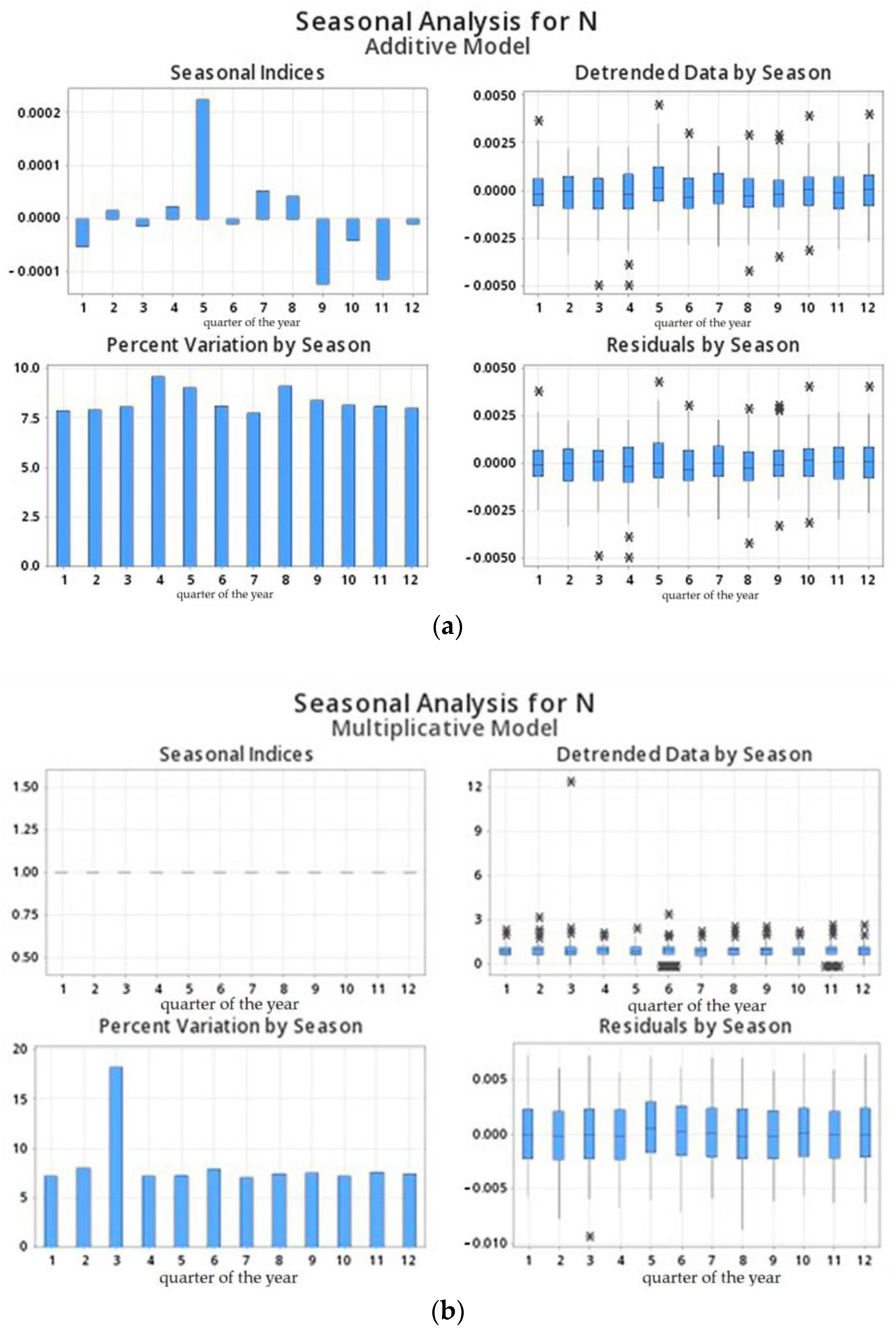
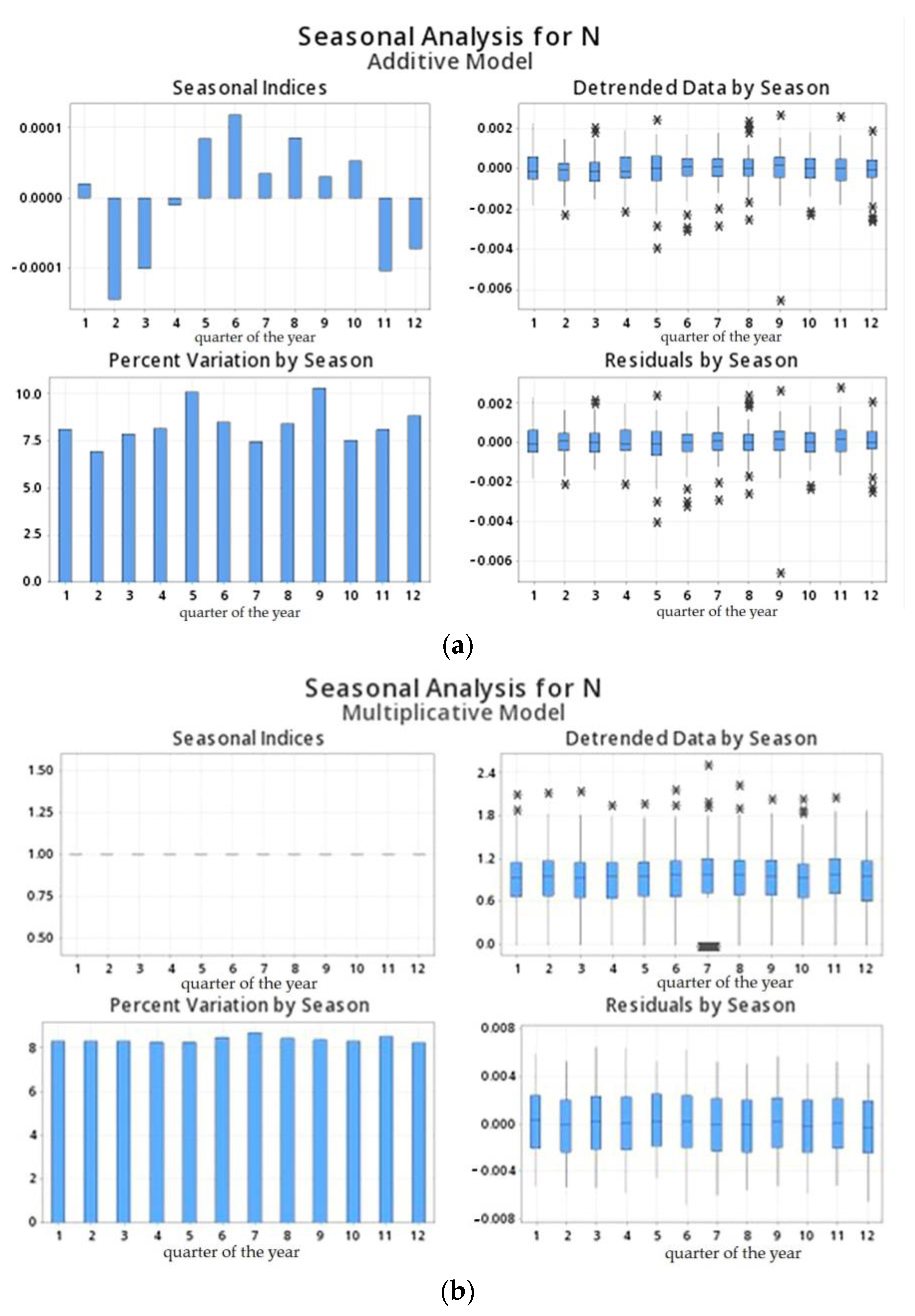
To investigate the presence of seasonal changes in the time series of coordinates, decomposition of the coordinate time series was performed using two methods (additive and multiplicative) [36] for two class C0 stations (POUS and CRAK) for data covering three years (2018–2020). The decomposition was held in four steps. In the first step, we smoothed the data using a centered moving average with a length equal to the length of the seasonal cycle. We then divided the moving average (a multiplicative model) and subtracted it from (the additive model) the data to obtain what is often referred to as raw seasonal values. For corresponding periods of time (a quarter of the year) in the seasonal cycles, we determined the median of the raw seasonal values. In our case we had 36 consecutive months of data (3 years), so we determined the median of the 12 raw seasonal values corresponding to winter (1, 5, 9), spring (2, 6, 10), summer (3, 7, 11), and fall (4, 8, 12). In the next step, we adjusted the medians of the raw seasonal values so that their average was one (multiplicative model) and zero (additive model). These adjusted medians constitute the seasonal indices. These indices were used to seasonally adjust the data. We then fit a trend line to the seasonally adjusted data using least squares regression. Figure 5 and Figure 6 show the results of decompositions (additive and multiplicative) for the POUS and CRAK stations.

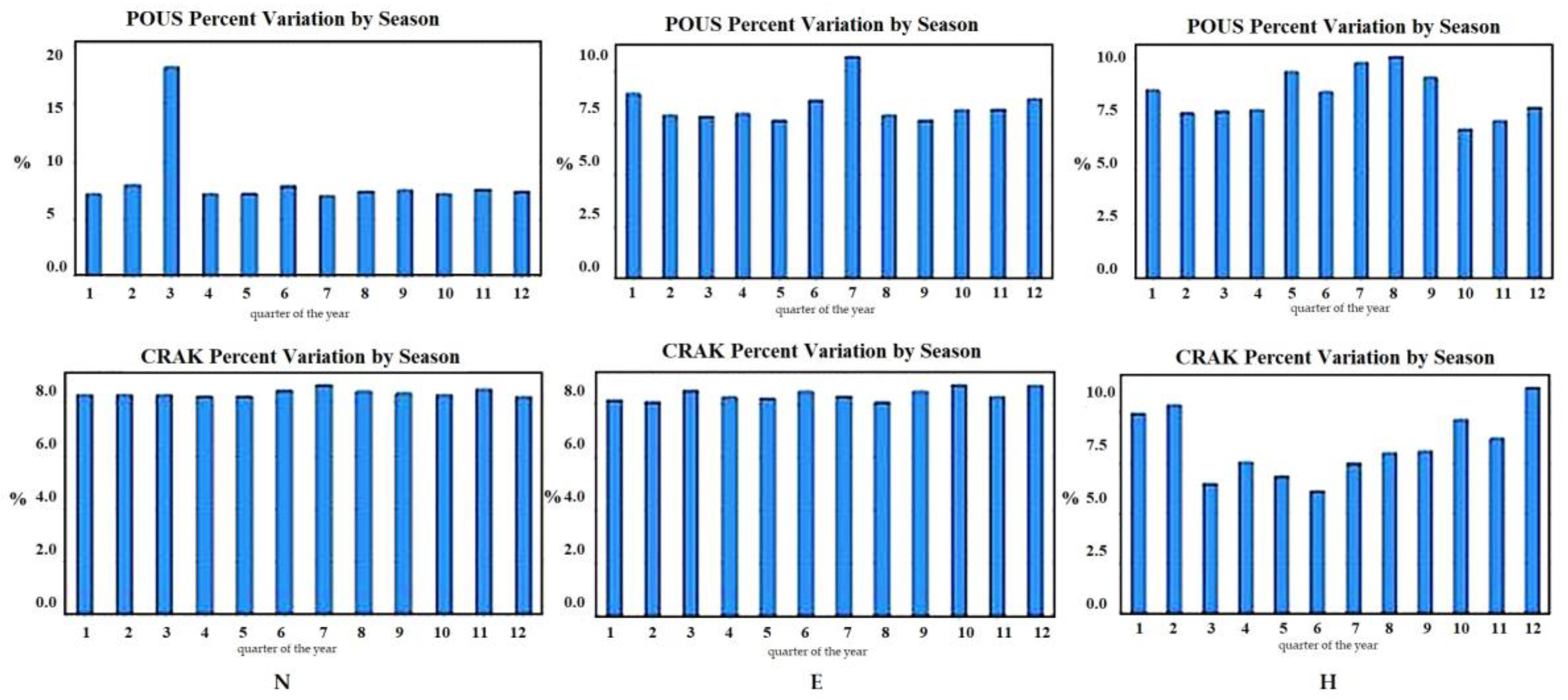
Figure 5 and Figure 6 show that the indices representing the seasonal component do not deviate from the value of 1 for the multiplicative decomposition and do not deviate from the value 0 for the additive decomposition; thus, it can be asserted that there are no seasonal variations in the quarters. Below are the percentage values of seasonal processes for each quarter for the POUS and CRAK stations.

From the diagrams (see Figure 7 and Figure 8), we can state that the seasonal component is not observed in the coordinate time series since it does not exceed 10% for additive decomposition and 20% for multiplicative decomposition. We can also claim that it is best to use the additive model for coordinate time series since seasonal fluctuations are relatively constant over time. None of the components of the time series had multiplicative properties (the values of seasonal variations did not increase over time).

The next step of our work was to check whether the obtained decomposition results were reliable. To do this, we repeated the decomposition of the coordinate time series for the POUS and CRAK stations using the RegARIMA model. Sample prediction of the sequence for 3 years in the forward and back directions was carried out using the RegARIMA model to supplement the data. A series of filters of different lengths were then constantly used for moving average operations, and various components such as seasonal, irregular, and trend recycling were extracted. Eventually, the results of seasonal adjustment for the POUS and CRAK stations were examined and showed in

Table 5. Statistics for seasonality for the POUS and CRAK stations using the RegARIMA model.

Station	Seasonality	Seasonal Values
POUS	0	1
CRAK	0	1

.

Indices representing the seasonal component do not deviate from the value of 1, so it can be argued that there are no seasonal variations. The obtained results confirm the absence of a seasonal component in the time series of the GNSS coordinates of the POUS and CRAK stations.

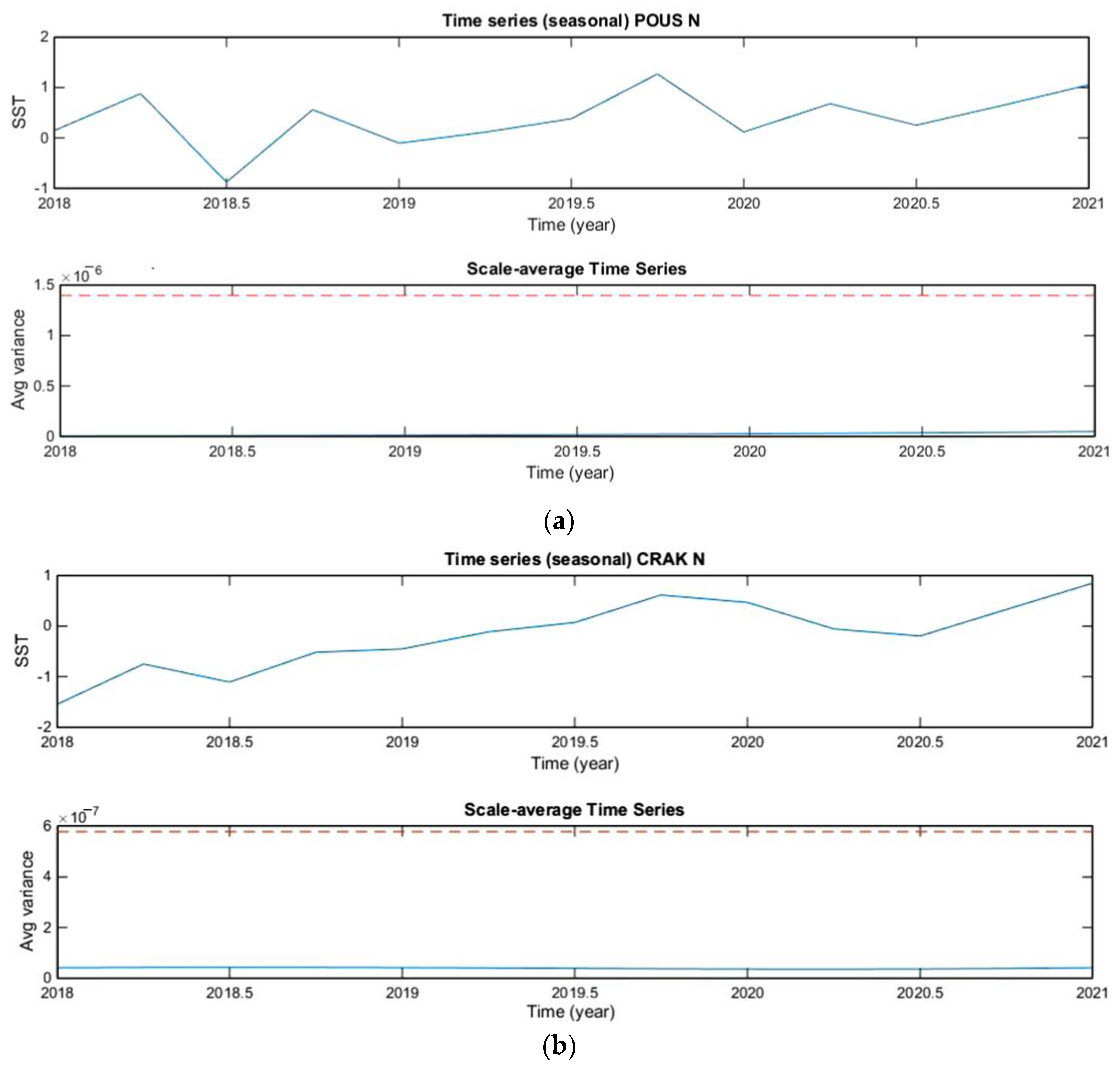
To check the presence of a seasonal component in the coordinate time series using the method of wavelet analysis, the MATLAB Wavelet Toolbox [37] was used. Similarly, as in the above two methods, the decomposition of coordinate time s was performed for stations POUS and CRAK, and two more stations (POLV and JOZ2) were additionally included for analysis. To examine fluctuations in power over a range of scales, the scale-averaged wavelet power was defined as the weighted sum of the wavelet power spectrum over the scales. By scale averaging the wavelet power spectra at multiple locations, one can assess a data field’s spatial and temporal variability.

From Figure 9, we can observe a certain seasonal component that corresponds to the four seasons. However, the amplitude of these oscillations is less than 2 mm. Data scale averaging of the wavelet power spectra shows that the temporal variability is so small (~0.5 × 10⁻⁶ mm) that we can consider it as the absence of seasonal fluctuations in the time series.

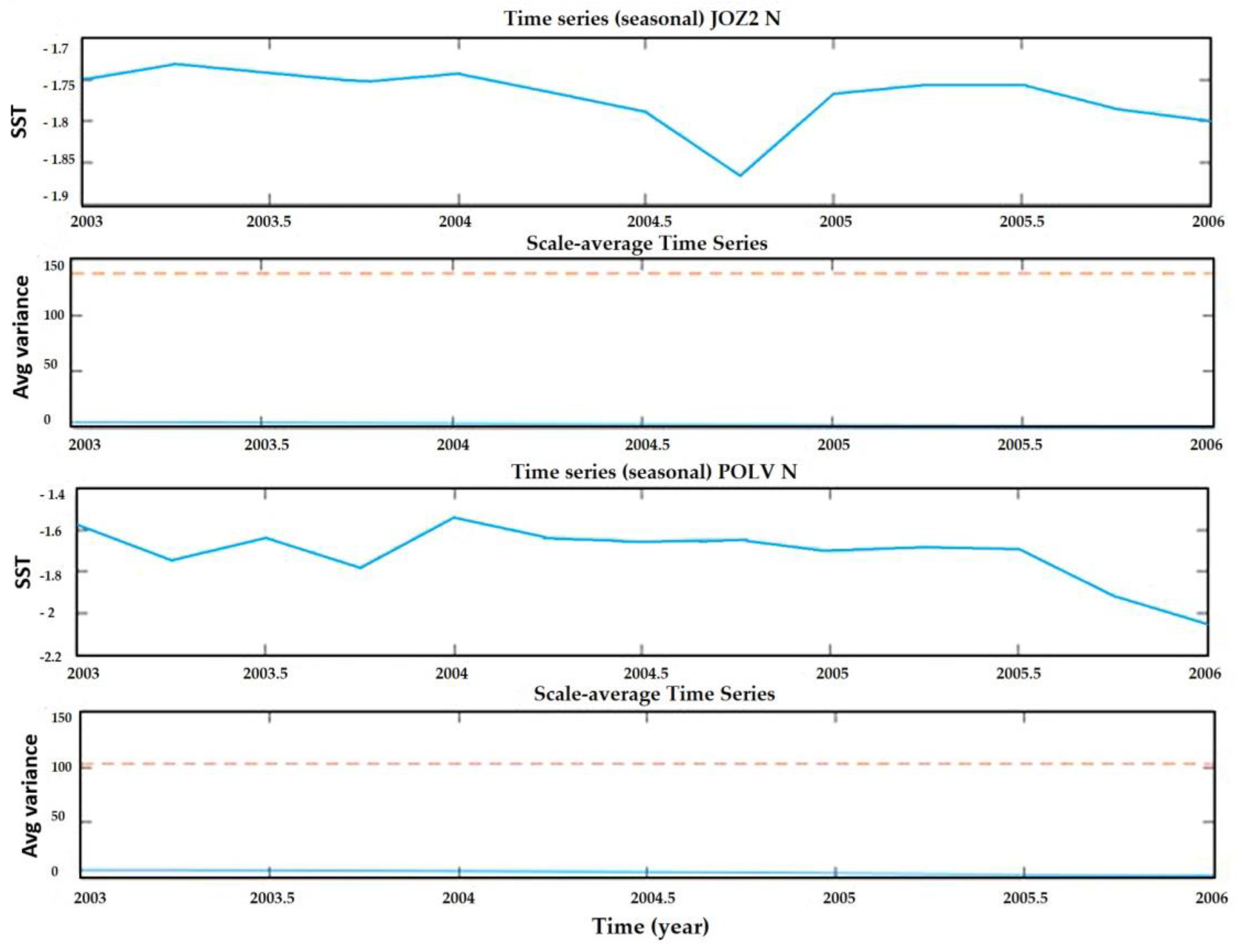
To check the absence of seasonal fluctuations in the stations, we chose another time interval of 2003–2005 (Figure 10).

From Figure 10, we can also observe a certain seasonal component that corresponds to the four seasons. However, the amplitude of these oscillations is less than 2 mm. Additionally, data scale averaging of the wavelet power spectra shows that the temporal variability is ~5–10 mm, so we can thus consider the presence of seasonal fluctuations in the time series.

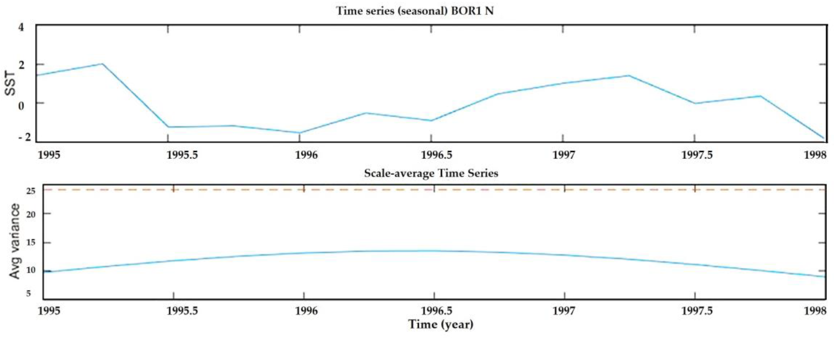
Since we received such results that confirmed the presence of seasonal fluctuations, we took another time interval of 1995–1997 and performed decomposition.

From Figure 11, we can also observe a certain seasonal component that corresponds to the four seasons, and the amplitude of these oscillations is less than 2 mm. The data scale averaging of wavelet power spectra shows that the temporal variability is ~10–15 mm, so we can also consider the presence of significant seasonal fluctuations in the time series.

4. Discussions and Conclusions

In this paper, the daily coordinate time series of 10 permanent GNSS stations in the central-eastern part of Europe from 2001 to 2019 were analyzed to improve the estimation of station motion parameters, particularly the determination of reliable velocity vectors together with their realistic uncertainties. First, the interpretation of discrepancies in the context of the individual accuracy of time series was carried out using the additional capabilities of the GAMIT/GLOBK software package. A seasonal signal with constant amplitude and phase in long GNSS time series was estimated with standard least squares parameters. Secondly, we estimated the percentage values of the residual seasonal processes in the cleaned time series based on the use of additive and multiplicative decomposition models and the RegARIMA model. The following conclusions can be drawn from our research.

The coefficients of seasonal variations from the sub-network of GNSS stations included in the C0–C1 category (Figure 4) are less than 1 mm. Thus, for the N component, the average value of the coefficients for the annual cycle and semi-annual cycle is −0.2 mm and 0.1 mm, respectively. For E, these values are −0.1 mm and 0.0 mm. For the altitudinal component, they are somewhat larger; the average value of the coefficients for the annual cycle is −0.6 mm and the average value for the semi-annual cycle −0.1 mm. As for the C6 sub-network, the average values of the coefficients of seasonal variations are significantly higher (up to 5 mm). This may be due to the specific features of the operation of such stations. We noted that with increases in the time interval of observations, the coefficients of seasonal variations for the stations in the C6 category decreased. Verification of the obtained results was carried out for four permanent C1 class stations (BRUX, CRAK, POUS, WARE) using EPN solutions based on Bernese GNSS Software. It showed that the differences in the coefficients of seasonal variations between the two solutions (GAMIT/GLOBK and Bernese) did not exceed 0.5 mm and were random.

Although the nonlinear component of the GNSS coordinate time series originating from seasonal periodic signals is not fully understood, a significant part of it should be attributed to the influence of Earth load effects, which either remain unmodeled during GNSS data processing or are partially compensated for by taking into account other factors. For example, modeling hydrostatic zenith tropospheric delays with mean or slowly varying empirical pressure values instead of actual pressure values leads to partial compensation of atmospheric loading. Thus, time series of GNSS coordinates based on an empirical meteorological model have better repeatability as a seasonal component than those based on more realistic tropospheric models, such as GPT2w, unless corrections for atmospheric loading are included.

Analysis of the presence of seasonal changes in the residual coordinate time series, which was also carried out according to the well-known decomposition procedure, showed that the seasonal component was not observed in the coordinate time series. Content did not exceed 10% for additive decomposition and 20% for multiplicative decomposition. Research has shown that the additive decomposition model is more suitable for the GNSS time series since none of the components of the time series had multiplicative properties (the values of seasonal variations did not increase over time). An additional check for the presence of seasonal changes carried out for two stations using another decomposition model, RegARIMA, only confirmed the previous conclusion.

Therefore, as stated in [4], coordinate time series are, by definition, trajectories; thus, fitting a trajectory model to these series in order to obtain accurate geophysical information with realistic error scales is extremely important. The factors underlying trajectory model search and selection approaches require further study.

References

1. Bos, M.S.; Bastos, L.; Fernandes, R.M.S. The influence of seasonal signals on the estimation of the tectonic motion in short continuous GPS time-series. J. Geodyn. 2010, 49, 205–209. [Google Scholar] [CrossRef] [Green Version]
2. He, X.; Montillet, J.-P.; Fernandes, R.; Bos, M.; Yu, K.; Hua, X.; Jiang, W. Review of current GPS methodologies for producing accurate time series and their error sources. J. Geodyn. 2017, 106, 12–29. [Google Scholar] [CrossRef]
3. Bock, Y.; Melgar, D. Physical applications of GPS geodesy: A review. Rep. Prog. Phys. 2016, 79, 106801. [Google Scholar] [CrossRef] [PubMed]
4. Montillet, J.P.; Bos, M. Geodetic Time Series Analysis in Earth Sciences; Springer Geophysics; Springer: Berlin/Heidelberg, Germany, 2020; 422p. [Google Scholar] [CrossRef]
5. Savchyn, I.; Brusak, I.; Tretyak, K. Analysis of recent Antarctic plate kinematics based on GNSS data. Geodesy Geodyn. 2023, 14, 99–110. [Google Scholar] [CrossRef]
6. Savchyn, I. Establishing the correlation between changes of absolute rotation poles of major tectonic plates based on continuous GNSS stations data. Acta Geodyn. Geomater. 2022, 19, 167–176. [Google Scholar] [CrossRef]
7. Haritonova, D. The Impact of the Baltic Sea Non-tidal Loading on GNSS Station Coordinate Time Series: The Case of Latvia. Balt. J. Mod. Comput. 2019, 7, 541–549. [Google Scholar] [CrossRef]
8. Wang, H.; Ren, Y.; Hou, Y.; Wang, J.; Zhang, Y.; Cheng, Y.; Xue, S.; Fang, S. The refinement of reprocessed GNSS three-decade displacement trajectory model with spectral analysis and hypothesis test. Adv. Space Res. 2022, 70, 1810–1829. [Google Scholar] [CrossRef]
9. Dvulit, P.; Savchuk, S.; Sosonka, I. Accuracy estimation of site coordinates derived from GNSS-observations by non-classical error theory of measurements. Geodesy Geodyn. 2021, 12, 347–355. [Google Scholar] [CrossRef]
10. Blewitt, G.; Lavallée, D. Effect of annual signals on geodetic velocity. J. Geophys. Res. Solid Earth 2002, 107, ETG 9-1–ETG 9-16. [Google Scholar] [CrossRef] [Green Version]
11. Bogusz, J.; Klos, A. On the significance of periodic signals in noise analysis of GPS station coordinates time series. GPS Solut. 2015, 20, 655–664. [Google Scholar] [CrossRef] [Green Version]
12. Dong, D.; Fang, P.; Bock, Y.; Cheng, M.K.; Miyazaki, S. Anatomy of apparent seasonal variations from GPS-derived site position time series. J. Geophys. Res. Solid Earth 2002, 107, ETG 9-1–ETG 9-16. [Google Scholar] [CrossRef] [Green Version]
13. Maciuk, K. The Study of Seasonal Changes of Permanent Stations Coordinates based on Weekly EPN Solutions. Artif. Satell. 2016, 51, 1–18. [Google Scholar] [CrossRef] [Green Version]
14. Larochelle, S.; Gualandi, A.; Chanard, K.; Avouac, J. Identification and Extraction of Seasonal Geodetic Signals Due to Surface Load Variations. J. Geophys. Res. Solid Earth 2018, 123, 11031–11047. [Google Scholar] [CrossRef]
15. Petit, G.; Luzum, B. IERS Conventions (2010); (No. IERS-TN-36); Bureau International des Poids et Mesures Sevres: Frankfurt am Main, Germany, 2010. [Google Scholar] [CrossRef]
16. Herring, T.A.; King, R.W.; Floyd, M.A.; McClusky, S.C. Introduction to GAMIT/GLOBK, Release 10.7. 2018, pp. 1–54. Available online: http://geoweb.mit.edu/gg/docs/Intro_GG.pdf (accessed on 27 July 2023).
17. Santamaría-Gómez, A. SARI: Interactive GNSS position time series analysis software. GPS Solut. 2019, 23, 52. [Google Scholar] [CrossRef]
18. Global Geophysical Fluid Center (GGFC). Available online: http://geophy.uni.lu (accessed on 27 July 2023).
19. Klos, A.; Bos, M.S.; Bogusz, J. Detecting time-varying seasonal signal in GPS position time series with different noise levels. GPS Solut. 2017, 22, 21. [Google Scholar] [CrossRef] [Green Version]
20. Langbein, J. Methods for Rapidly Estimating Velocity Precision from GNSS Time Series in the Presence of Temporal Correlation: A New Method and Comparison of Existing Methods. J. Geophys. Res. Solid Earth 2020, 125, e2019JB019132. [Google Scholar] [CrossRef]
21. Santamaría-Gómez, A.; Bouin, M.-N.; Collilieux, X.; Wöppelmann, G. Correlated errors in GPS position time series: Implications for velocity estimates. J. Geophys. Res. Atmos. 2011, 116, e2010jb007701. [Google Scholar] [CrossRef]
22. Kudrys, J. Spectral analysis of multi-year GNSS code multipath time-series. Bud. i Arch. 2020, 18, 15–22. [Google Scholar] [CrossRef]
23. Ren, Y.; Wang, H.; Lian, L.; Wang, J.; Cheng, Y.; Zhang, Y.; Zhu, W.; Zhang, S. A method based on MTLS and ILSP for GNSS coordinate time series analysis with missing data. Adv. Space Res. 2021, 68, 3546–3561. [Google Scholar] [CrossRef]
24. Amiri-Simkooei, A.R. Non-negative least-squares variance component estimation with application to GPS time series. J. Geod. 2016, 90, 451–466. [Google Scholar] [CrossRef]
25. Tian, Y.; Shen, Z.-K. Extracting the regional common-mode component of GPS station position time series from dense continuous network. J. Geophys. Res. Solid Earth 2016, 121, 1080–1096. [Google Scholar] [CrossRef]
26. Agnieszka, W.; Kudas, D. Modeling seasonal oscillations in GNSS time series with Complementary Ensemble Empirical Mode Decomposition. GPS Solut. 2022, 26, 101. [Google Scholar] [CrossRef]
27. Chen, Q.; van Dam, T.; Sneeuw, N.; Collilieux, X.; Weigelt, M.; Rebischung, P. Singular spectrum analysis for modeling seasonal signals from GPS time series. J. Geodyn. 2013, 72, 25–35. [Google Scholar] [CrossRef]
28. Gruszczynska, M.; Rosat, S.; Klos, A.; Gruszczynski, M.; Bogusz, J. Multichannel Singular Spectrum Analysis in the Estimates of Common Environmental Effects Affecting GPS Observations. Pure Appl. Geophys. 2018, 175, 1805–1822. [Google Scholar] [CrossRef] [Green Version]
29. Chen, B.; Bian, J.; Ding, K.; Wu, H.; Li, H. Extracting Seasonal Signals in GNSS Coordinate Time Series via Weighted Nuclear Norm Minimization. Remote Sens. 2020, 12, 2027. [Google Scholar] [CrossRef]
30. Jiang, W.; Ma, J.; Li, Z.; Zhou, X.; Zhou, B. Effect of removing the common mode errors on linear regression analysis of noise amplitudes in position time series of a regional GPS network & a case study of GPS stations in Southern California. Adv. Space Res. 2018, 61, 2521–2530. [Google Scholar] [CrossRef] [Green Version]
31. Stallone, A.; Cicone, A.; Materassi, M. New insights and best practices for the successful use of Empirical Mode Decomposition, Iterative Filtering and derived algorithms. Sci. Rep. 2020, 10, 15161. [Google Scholar] [CrossRef]
32. Chen, G.; Zhao, Q.; Wei, N.; Liu, J. Impacts on Noise Analyses of GNSS Position Time Series Caused by Seasonal Signal, Weight Matrix, Offset, and Helmert Transformation Parameters. Remote Sens. 2018, 10, 1584. [Google Scholar] [CrossRef] [Green Version]
33. Böhm, J.; Moeller, G.; Schindelegger, M.; Pain, G.; Weber, R. Development of an improved empirical model for slant delays in the troposphere (GPT2w). GPS Solut. 2015, 19, 433–441. [Google Scholar] [CrossRef] [Green Version]
34. EPN Solutions. Available online: https://epncb.oma.be/ (accessed on 27 July 2023).
35. U.S. Census Bureau. X-13ARIMA-SEATS Seasonal Adjustment Program. 2022. Available online: https://www.census.gov/data/software/x13as.Win_X-13.html#list-tab-635278563 (accessed on 27 July 2023).
36. Minitab. Statistical Software. 2022. Available online: https://www.minitab.com/en-us/products/minitab/ (accessed on 27 July 2023).
37. MATLAB Wavelet Toolbox. Available online: https://www.mathworks.com/products/wavelet.html (accessed on 27 July 2023).
Figure 1. Standard processing of observations in the GAMIT/GLOBK v.10.71 software [16].
Remotesensing 15 03858 g001
Figure 2. The processing network of GNSS stations used for the ITRF2014 realization.
Remotesensing 15 03858 g002
Figure 3. Topocentric coordinate time series of station CRAK.
Remotesensing 15 03858 g003
Figure 4. EPN subnets: red triangles—GNSS stations of class C0–C1, black triangles—GNSS stations of class C6.
Remotesensing 15 03858 g004
Figure 5. Results of (a) additive and (b) multiplicative decomposition for the POUS station.
Remotesensing 15 03858 g005
Figure 6. Results of (a) additive and (b) multiplicative decomposition for the CRAK station.
Remotesensing 15 03858 g006
Figure 7. Percentage values of seasonal processes for each quarter for the POUS and CRAK stations in the northern (N), eastern (E), and height (H) components from the additive decomposition.
Remotesensing 15 03858 g007
Figure 8. Percentage values of seasonal processes for each quarter for the POUS and CRAK stations in the northern (N), eastern (E), and height (H) components from the multiplicative decomposition.
Remotesensing 15 03858 g008
Figure 9. Results (in mm) of wavelet decomposition for stations (a) POUS, (b) CRAK, (c) POLV, and (d) JOZ2 for the time interval 2018–2020.
Remotesensing 15 03858 g009aRemotesensing 15 03858 g009b
Figure 10. Results (in mm) of wavelet decomposition for stations POLV and JOZ2 for the time interval 2003–2005.
Remotesensing 15 03858 g010
Figure 11. Results (in mm) of wavelet decomposition for stations POLV and JOZ2 for the time interval 1995–1997.
Remotesensing 15 03858 g011