Article

Method of Development of a New Regional Ionosphere Model (RIM) to Improve Static Single-Frequency Precise Point Positioning (SF-PPP) for Egypt Using Bernese GNSS Software

1
Faculty of Engineering, Aswan University, Aswan 81528, Egypt
2
Institute of Engineering Geodesy (IIGS), Stuttgart University, 70174 Stuttgart, Germany
3
Egyptian Surveying Authority, Orman P.O. Box 63, Giza 12612, Egypt
*
Author to whom correspondence should be addressed.
Remote Sens. 2023, 15(12), 3147; https://doi.org/10.3390/rs15123147
Submission received: 28 April 2023 / Revised: 29 May 2023 / Accepted: 1 June 2023 / Published: 16 June 2023
(This article belongs to the Special Issue GNSS CORS Application)

Abstract

:
Due to the lack of coverage of IGS in Africa, especially over North Africa, and the construction revolution of infrastructure in Egypt, a geodetic CORS stations network was established in 2012. These CORS stations are operated by the Egyptian Surveying Authority (Egy. SA) and cover the whole of Egypt. The paper presents a fully developed regional ionosphere model (RIM) depending on the Egyptian CORS stations. The new model and the PPP solution were obtained using Bernese GNSS V. 5.2 software. An observation data series of eight days (DOY 201–208)/2019 was used in this study. Eighteen stations were used to develop the RIM model for each day; fifteen stations were used to validate the new RIM model. A static SF-PPP solution was obtained using the CODE-GIM and RIM models. Comparing the outcomes to the reference network solution, based on the recently developed RIM model, the solution showed a mean error of 0.06 m in the East direction, 0.13 m in the North direction, and 0.21 m in the height direction. In the East, North, and height directions, this solution improves the SF-PPP result achieved by the Global Ionosphere Maps (CODE-GIM) model by 60%, 68%, and 77%, respectively.

1. Introduction

According to ref. [1], the ionosphere layer is based on solar activity and the geomagnetic field; moreover, it is extended from 50 km to 1100 km above the Earth’s surface. The frequency, location, and time affect the ionosphere’s refraction range. For the lowest ionosphere activity and the highest activities, the error propagation approaches 1–2 m and 10–50 m, respectively [1]. Total Electron Content (TEC), which refers to the total number of electrons along the line path between the satellite and the receiver, is a key factor in defining ionosphere refraction ref. [2]. The ionosphere error mitigation for dual-frequency (DF-PPP) solution is mainly based on the first-order free linear ionosphere combination. In the case of the single-frequency (SF-PPP), solutions are primarily facing the error of ionosphere refraction error. To model the ionosphere error, many different models have been created. Klobuchar’s model, which is based on a set of parameters broadcast to user receivers as a part of the navigation message, decreases the ionospheric error by 50% ref. [3]. Vertical TEC (VTEC) maps, also known as final global ionosphere maps (GIM), have been made available by the International GNSS Services (IGS) since 1998. The IONospheric Exchange (IONEX) format is used to deliver the ionosphere products [4]; visit [5] to access them. IGS-GIM products contain VTEC values with a spatial resolution of 2.5° for latitude and 5° for longitude, and 2 h as a temporal resolution. The final result has an accuracy of 2–8 TECU and a latency of approximately 11 days (on L1 frequency, 1 TECU is equivalent to 0.16 m of delay) ref. [6].
International Reference Ionosphere (IRI) is a popular empirical ionosphere model that gives a worldwide description of the ionospheric electron density and other characteristics as a function of altitude, latitude, and time. It is based on a sizable database of ionospheric observations collected from numerous sources, and it is frequently updated to take into account fresh information and new modeling strategies ref. [7]. The European Space Agency (ESA) and the International Union of Radio Science (URSI) developed NeQuick, an empirical ionosphere model. Ionospheric modeling makes extensive use of it, especially at mid-to-low latitudes. Based on a regional strategy that considers local ionospheric conditions, the NeQuick model determines the ionospheric electron density as a function of altitude, latitude, and time using a number of techniques. Solar activity, geomagnetic storms, and ionospheric disturbances are just a few of the variables that the model takes into account when predicting how the ionosphere will behave. Compared to other models of the ionosphere, the NeQuick model provides a number of benefits. For instance, it is effective computationally and has real-time applications. Additionally, as the ionosphere is more complicated and varied at mid-to-low latitudes than it is at higher latitudes, it is ideally suited for modeling the ionosphere at these latitudes refs. [8,9,10].
Researchers have developed a number of ionosphere models, e.g., refs. [11,12,13,14,15,16,17,18,19,20]. Using real-time products from IGS, ref. [21] developed a regional ionosphere model in real-time (RT-RIM) for Europe. The model had a spatial resolution of 1° × 1° and a temporal resolution of 15 min. The Bernese GNSS V. 5.2 PPP module was used to analyze 60 IGS and EUREF reference stations to extract the Real-Time VTEC values. The proposed model showed an improved SF-PPP accuracy under the mid-latitude region when compared to the IGS-GIM, with respect to the horizontal, vertical, and 3D components, of about 40%, 55%, and 40%, respectively.
Using 56 CORS stations for Turkey and 12 IGS stations for processing, ref. [13] determined the TEC values on a regional scale. Using Bernese GNSS V. 5.2 software, the TEC values were computed with a two-hour interval for the phase measurements ( L 4 ). The data were compared using GIM information from the International Reference Ionosphere (IRI)) ref. [7], the European Space Operations Centre (ESOC), the Jet Propulsion Laboratory (JPL), and CODE (Centre for Orbit Determination in Europe, Switzerland) ref. [22].
Ref. [23] assessed the SF-PPP solution for 40 multi-GNSS stations worldwide distributed for a one-week data set in October 2020, achieving 0.1 m and 0.2 m horizontal and vertical position accuracy. Ref. [24] developed the regional ionosphere model (RIM) for Australia using 40 multi-GNSS stations. The SF-PPP solution using RIM and a CODE-GIM model-delivered solution were compared. According to experimental data, utilizing the regional model enhanced the position performance by 15% to 18%. Additionally, the improvement reached 28–35% during the active ionosphere period.
Using the L 4 linear phase combination, ref. [25] modeled a regional ionosphere model for the Nile Delta in Egypt using an algorithm. The study estimated the VTEC values and compared them to CODE-GIM values. The Bernese GNSS V. 5.0 PPP model generated the regional ionosphere maps for quiet and stormy days. Due to the lack of IGS stations in North Africa, the results of the CODE-GIM model are not as accurate as those of the VTEC model, which is based on three CORS stations that constitute the Nile Delta in Egypt. For more case studies, see refs. [26,27,28], who created a regional ionosphere model (RIM) for Egypt’s delta using nine CORS stations over a period of six consecutive days, 202–207/2019. This model has a spatial resolution of 2.5° × 5° and a temporal resolution of 2 h. Five more CORS stations were processed with the RIM and CODE-GIM models for validation. The SF-PPP results displayed mean errors of 0.06 m, 0.10 m, and 0.30 m, respectively, in the East, the North, and height. This method outperformed the CODE-GIM model by 60%, 70%, and 67% in the East, North, and height, respectively.
As seen in Figure 1, due to the IGS network’s limited coverage in North Africa, the Egyptian Surveying Authority created the first permanent Egyptian reference station network in January 2012. This paper aims to develop a regional ionosphere for the whole of Egypt using Bernese GNSS software V. 5.2. A data set of 33 Egy. SA-CORS stations for DOY (201–208/2019) have been used to develop the new RIM model for Egypt. For model development, 18 stations were utilized to estimate the regional model. These stations cover the margins of Egypt: BALM in the North, EDFO in the South, ALEX in the West, and QANT in the East. For validation, 15 stations were processed in SF-PPP mode for 24 h as an observation time.

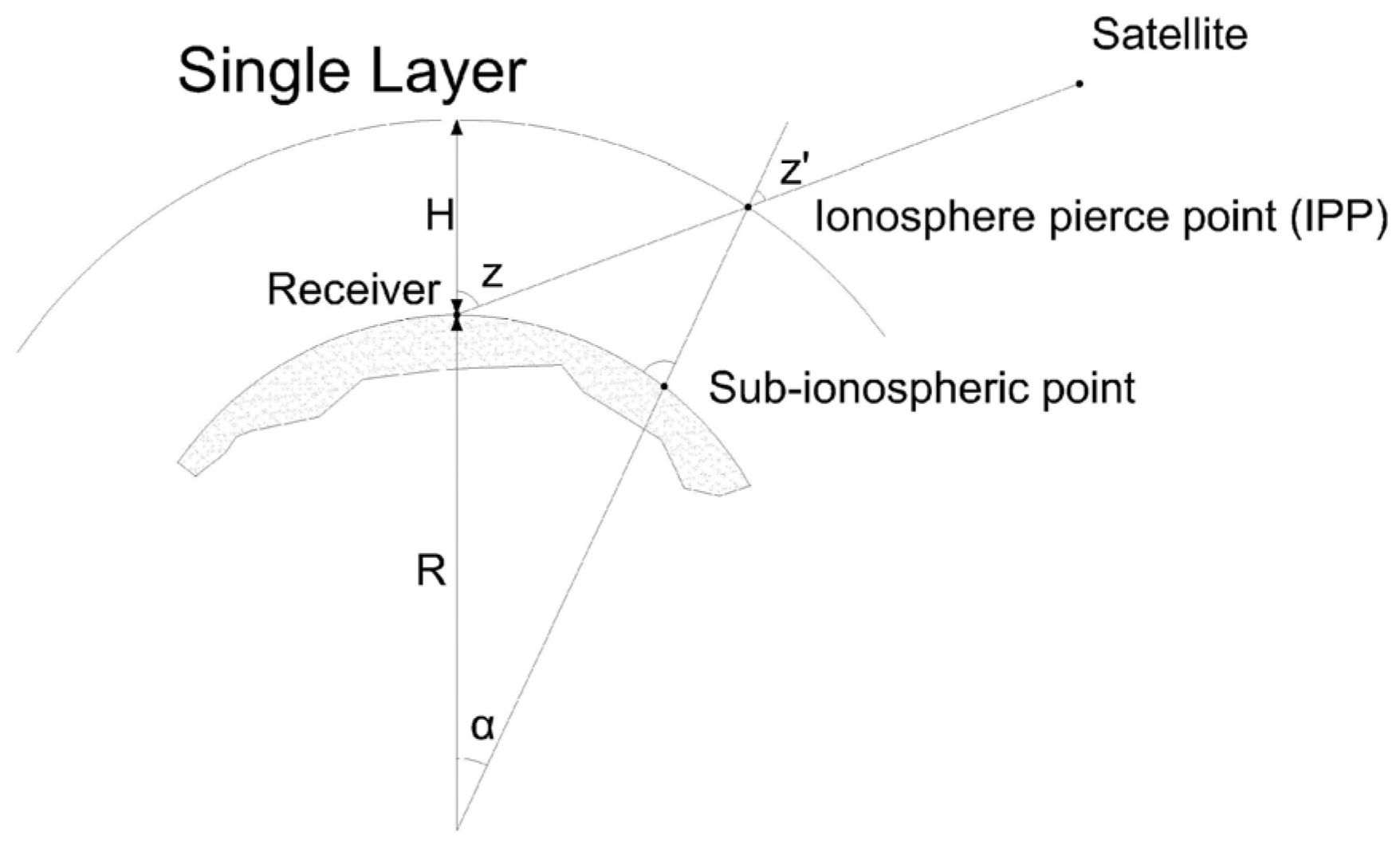
2. Ionosphere Modeling

Equations (1)–(4) are the fundamental GPS observation equations. The pseudo-range measurements for L 1 and L 2 carrier frequencies are P 1 and P 2 . Additionally, Φ 1 and Φ 2 refer to the carrier phase measurements for L 1 and L 2 [30].
P 1 = r R S + c δ R δ S + R I , 1 S + R T S + s o l + p o l + o c n + a t m + m u l + ϵ ρ
P 2 = r R S + c δ R δ S + R I , 2 S + R T S + s o l + p o l + o c n + a t m + m u l + ϵ ρ
Φ 1 = r R S + c δ R δ S R I , 1 S + R T S + λ 1 N 1 + s o l + p o l + o c n + a t m + p c v + m u l + λ 1 w + ϵ Φ
Φ 2 = r R S + c δ R δ S R I , 2 S + R T S + λ 2 N 2 + s o l + p o l + o c n + a t m + p c v + m u l + λ 2 w + ϵ Φ
where c is the speed of light in the vacuum, and δ S are the receiver and satellite clock bias. λ 1 and λ 2 refer to the carrier wavelength for L 1 and L 2 carrier frequencies; N 1 and N 2 are the ambiguity integer for L 1 and L 2 carrier frequencies. R T S refers to the correction due to the ionosphere and troposphere refraction. s o l , p o l , o c n , a t m , m u l , p c v , and w are the correction for the solid Earth tides, pole tides, ocean loading, atmosphere loading, multipath effect, antenna phase offset and variation, and phase wind-up, respectively. In addition, ϵ ρ , and ϵ Φ denote the remaining un-modelled errors for code and phase noise. The true geometric range in meters is provided in Equation (5) as r R S .
r R S = x S x R 2 + y S y R 2 + z S z R 2 .
where x S , y S , and z S refer to satellite coordinates, and x R , y R , and z R are the antenna coordinates.
As can be seen in Figure 2, the ionosphere layer is an ionised Single-Layer Model (SLM) with gases [2]. This model is considered a concentrated free electron column in a shell of height ( H ) as seen in the figure below. The SLM mapping function ( F I ) is a function of the layer’s electron density ( E ) that is indicated in Equations (6) and (7) ref. [31].
F I z = E E v = 1 c o s   ( z )
sin z = R R + H sin   ( z )
α = z z
R is the mean radius of the Earth; H is the height of a single layer above the Earth’s surface (~300–500 km). z and z are the satellite zenith distances at the station’s height (receiver on Earth) and the single layer’s satellite zenith distance (IPP), respectively. Furthermore, α mentions the geocentric angle.
Based on ref. [32], the SLM mapping function was updated to the modified SLM that is expressed as (MSLM) by introducing an additional constant ( α ); Equation (7) is given as Equation (9).
sin z = R R + H sin   ( α z )
Ref. [31] indicated that the best match of MSLM according to JPL was H = 506.7   k m and α = 0.9782 when using R = 6371   k m , with a maximum zenith distance of 80°. This modified mapping function was used in the CODE analysis with H = 450   k m of the ionospheric pierce points (IPP).
To estimate the TEC values, a geometry-free linear combination of the un-differenced code ( P 4 ) and carrier-phase ( Φ 4 ) observations was used. This combination removes the terms of the geometrical, receiver, and satellite clock errors, as well as tropospheric delay. The code combination includes both the receiver’s and the satellite’s differential code bias (DCB). The ionospheric delay and the ambiguity parameters are also included in the carrier phase combination ref. [31].
P 4 = P 1 P 2 = + a 1 f 1 2 1 f 2 2 F I z E β , s + c ( b S + b R )
Φ 4 = Φ 1 Φ 2 = a 1 f 1 2 1 f 2 2 F I z E β , s + ( λ 1 N 1 λ 2 N 2 )
As seen in the relevant Equations (10) and (11), ( a ) is a constant with a value of 4.03 · 10 17 m s 2 V T E C 1 , F I z refers to the mapping function at the zenith distance ( z ), E β , s is the vertical TEC (VTEC) as a function of geographic or geomagnetic latitude ( β ) and sun-fixed longitude ( s ) of IPP. b S and b R are the differential code bias (DCB) for satellite and receiver. ( λ 1 N 1 λ 2 N 2 ) mentions the constant bias in the meter as an initial phase ambiguity.
The global and regional TEC model, as stated in ref. [31], is defined as a function of a spherical harmonic expansion ( E β , s ), the estimation details of which may be found in refs. [32,33]. Then, the TEC model whether global or regional can be expressed as:
E β , s = n = 0 n m a x m = 0 n P ~ n m sin   β ( a n m   c o s m · s + b n m   s i n m · s )
P ~ n m = ( n , m ) P n m
where n m a x is the spherical harmonic expansion’s maximum degree. P ~ n m are the normalized associated Legendre functions of degree n and order m , based on the normalization function ( n , m ) and Legendre functions P n m . a n m and b n m are the unknown TEC coefficients of the spherical harmonics to be estimated.

3. Regional Ionosphere Modelling Using Bernese GNSS Software V. 5.2

In this study, 18 Egy. SA-CORS stations were used to create the regional ionosphere model (RIM) for Egypt utilizing Bernese GNSS software that was developed at the Astronomical Institute of the University of Bern (AIUB), Switzerland. In addition, to obtain the SF-PPP solution, 15 Egy. SA-CORS stations were used as validation for the RIM model. The following parameters were obtained from the official FTP server of CODE under [ftp://ftp.aiub.unibe.ch/, accessed on 27 April 2023], as shown in Table 1. These files, which were adapted to each observation day of the campaign, were accessed throughout the entire processing phase using Bernese GNSS software.
The analysis during the study using Bernese GNSS software has three stages, as follows:

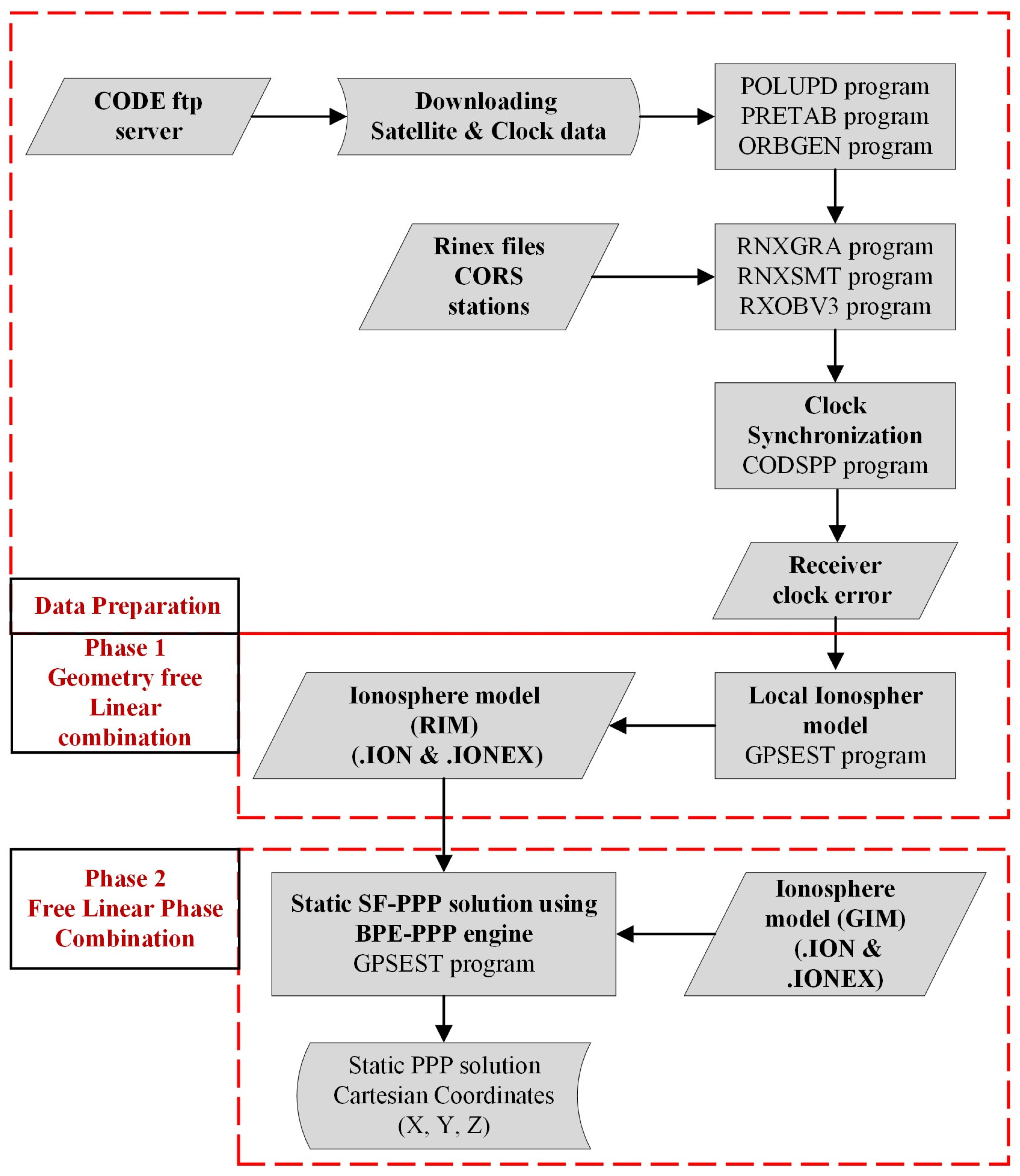
3.1. Data Preparations

This stage includes downloading the processing data that are shown in the previous table, in addition to orbit data preparations and RINEX data preprocessing, cleaning, and smoothing. Further details are explained in [28].
  • POLUPD program: to convert the earth pole information file to internal Bernese software format.
  • PRETAB program: to tabulate information about satellite orbit and atomic clocks.
  • ORBGEN program: to obtain standard orbit format.
  • RNXGRA program: to check the quality of Rinex data.
  • RNXSMT program: to remove cycle slips and outliers from phase and code files.
  • RXOBV3 program: converts the Rinex data that has been smoothed into Bernese binary format.
  • CODSPP program: to calculate the receiver clock error δ R based on the code combination P 3 using least-squares adjustment theory. The estimated δ R is afterwards added as a known value into the final coordinate’s estimation for static or kinematic; the mathematical model is explained in detail in [34].

3.2. Phase 1 [Geometry-Free Linear Combination (RIM Modelling)]

The regional ionosphere model (RIM) is generated via a geometry-free code linear combination using Bernese GNSS software. The zero-difference code observation data are added to the GPSEST program along with the DCB file. The following Table 2 shows the parameters used for RIM modelling. These parameters are highly recommended, according to [31].

3.3. Phase 2 [SF-PPP Solution]

The GPSEST program gives the static SF-PPP solution utilizing the Bernese processing engine (BPE-PPP). As shown in Figure 3, the solution is obtained twice; the first using the CODE-GIM model and the second using the modeled one. The final coordinates are obtained in Cartesian format, then converted to ellipsoidal and projected formats to be compared with the reference solution for Egy. SA-CORS stations.

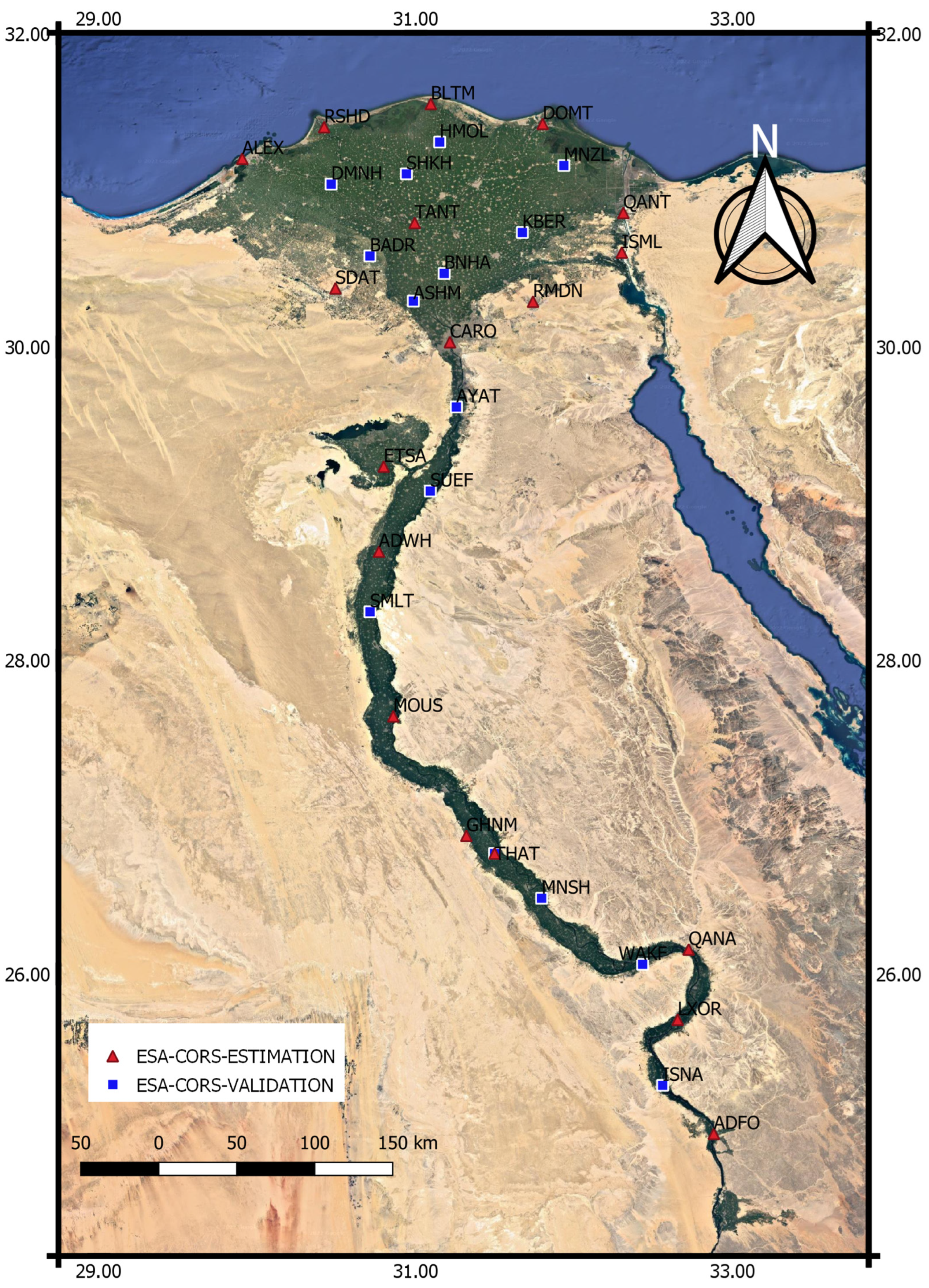
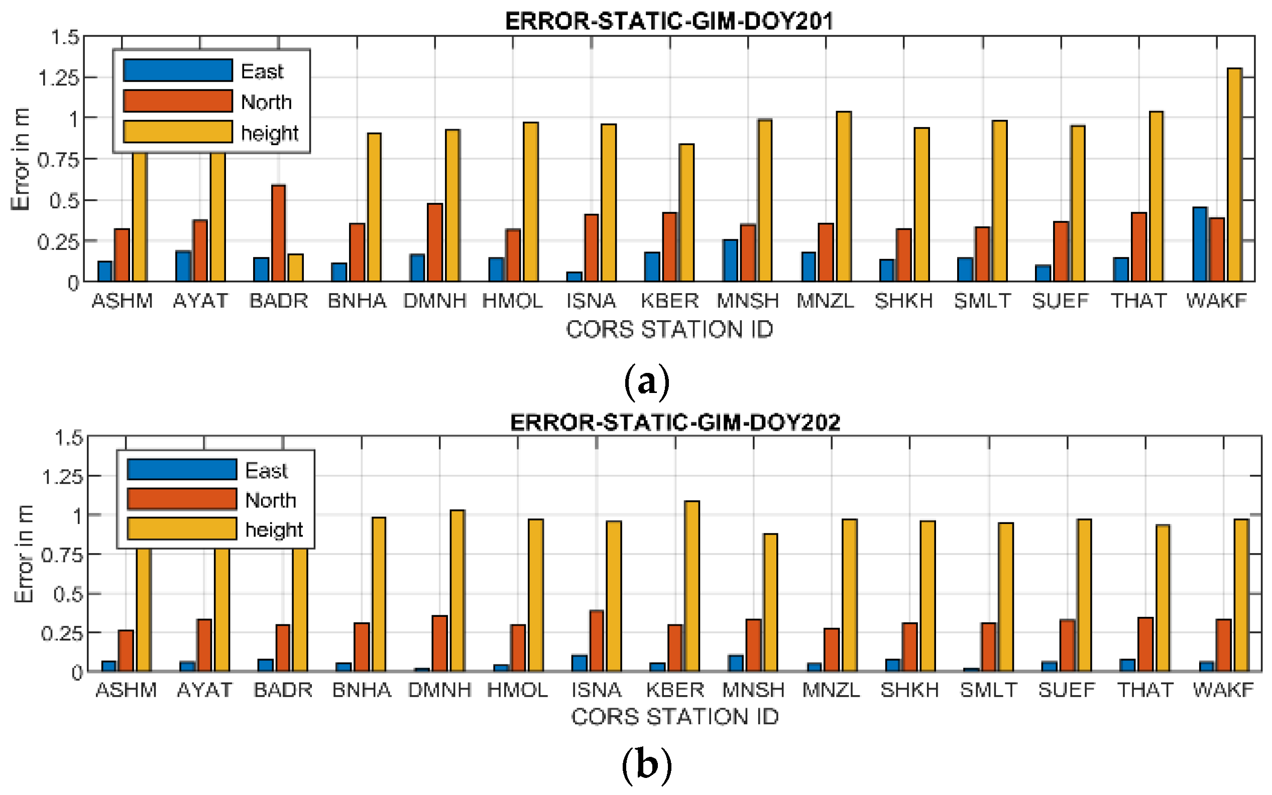
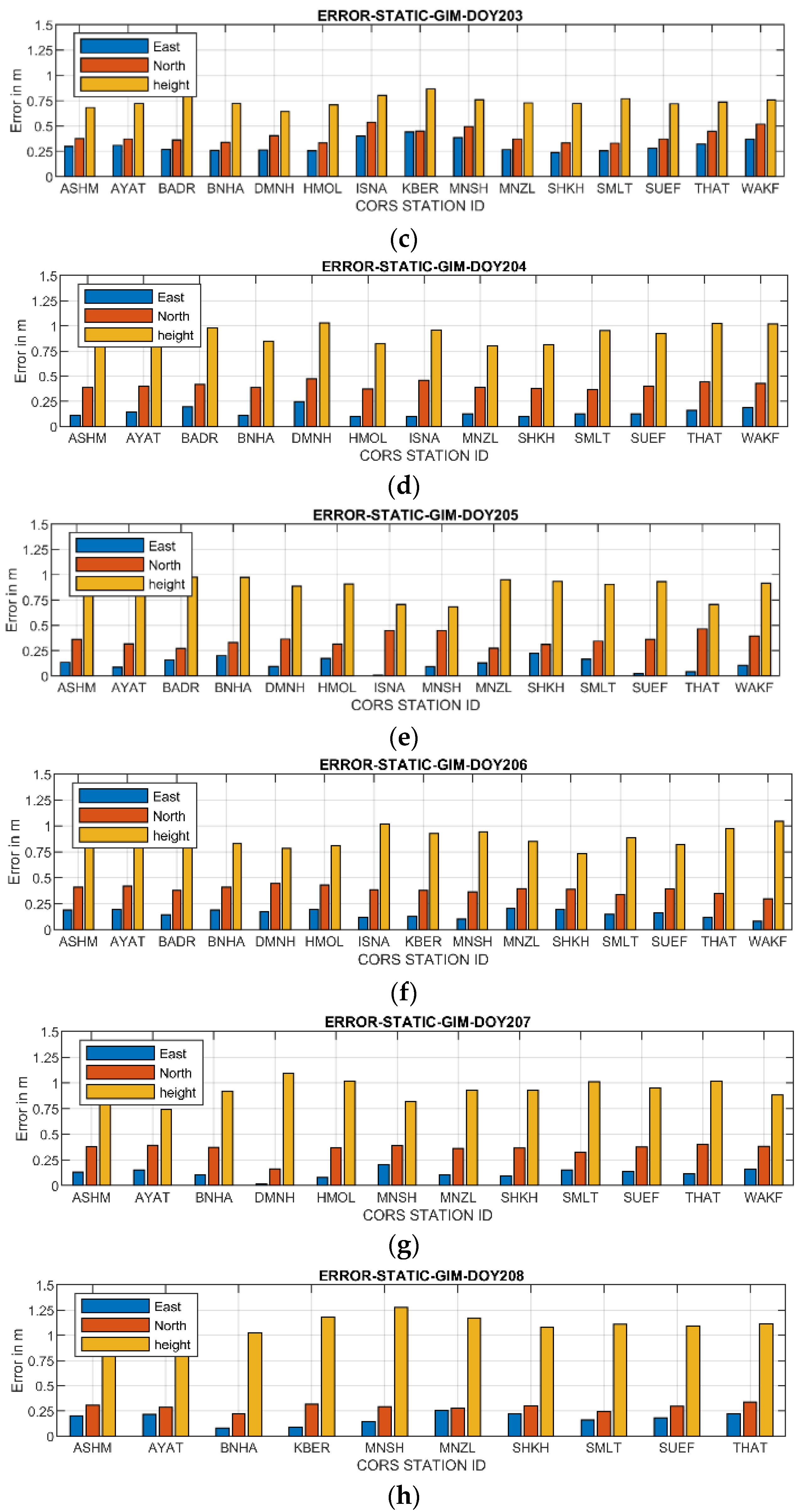
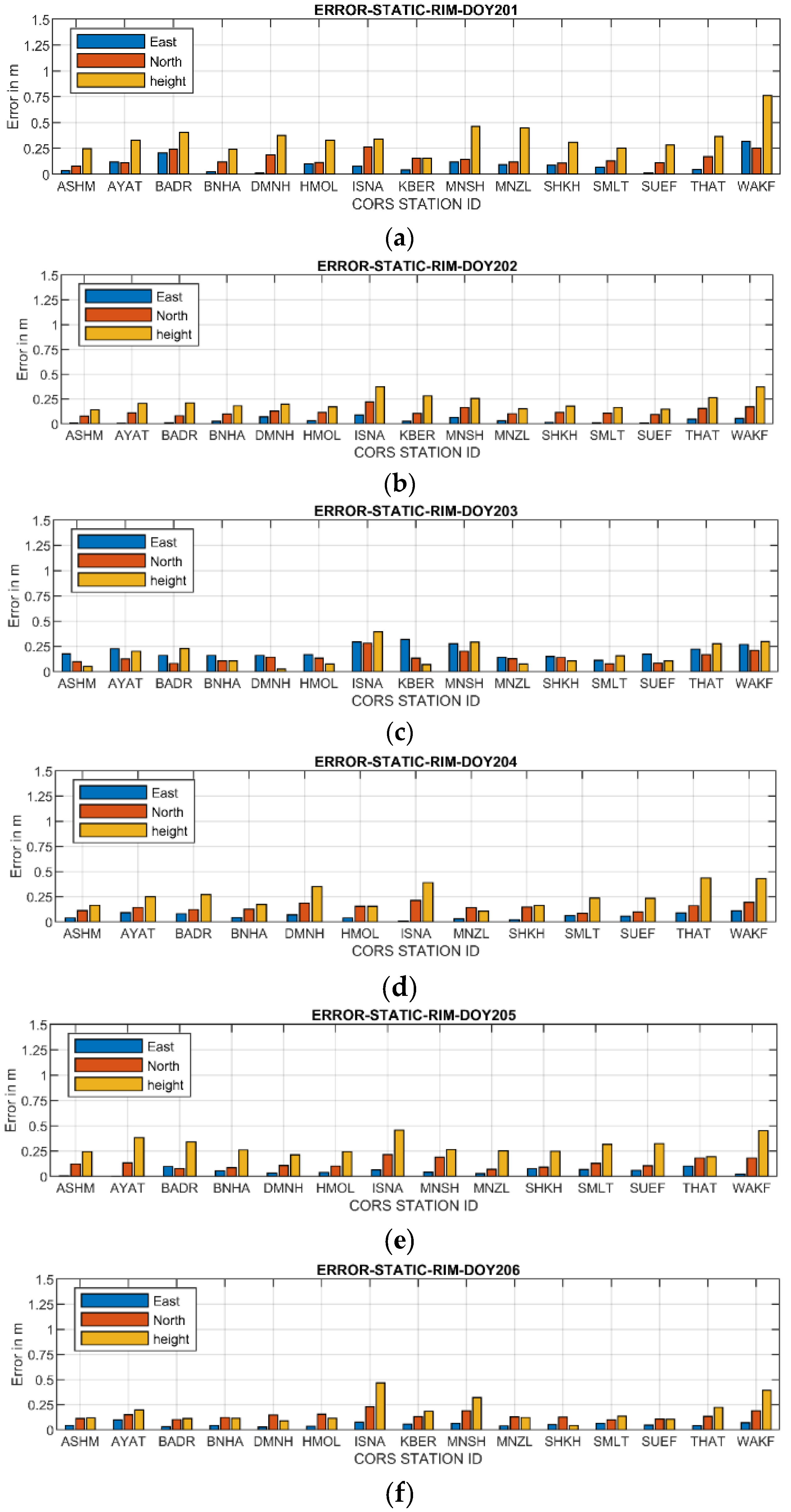
4. Evaluation Process

In order to evaluate the regional ionosphere model (RIM) for Egypt, 33 Egy. SA-CORS stations were included in the study for eight successive days, 201–208/2019. Eighteen stations were used for the regional ionosphere modelling for Egypt that cover the Nile delta and the valley (triangle mark). In addition, 15 stations were solved in SF-PPP mode (square mark). Using the Trimble Business Center (TBC) GNSS V. 5.2 software [35], the reference network solution was obtained in two steps: (i) six IGS-CORS (NICO, NKLG, NOT1, YKRO, DYNG, and RAMO) and six Egy. SA-CORS stations (CARO, MOUS, QANT, ADFO, ALEX, and SUZE) were tied; and (ii) based on the previous six Egy. SA-CORS stations, a locally constrained network solution was produced for the remaining stations; all relevant information regarding the reference solution is provided in refs. [36,37]. Figure 4 shows the IGS-CORS and Egy. SA-CORS stations that used for obtaining the reference solution. Figure 5 presents the total Egy. SA CORS stations that have been used in the study.
Table 3 shows the availability of Rinex observation data for the validation stations throughout the study period. For DOY 201–203 and DOY 206, the data are available for all validated CORS stations. For the stations KBER and MNSH, the Rinex data are missing for DOY 204. Further, station MNSH data are missing for DOY 205. Three stations (BADR, ISNA, and KBER) are missing for DOY 207; unfortunately, six stations were lost for the final day of observation data (BADR, DMNH, HMOL, ISNA, KBER, and WAKF). The possible explanation for losing the observation data is the poor Global System for Mobile Communications (GSM) transfer from CORS stations to the data center in Cairo, as explained in ref. [36].

5. Results

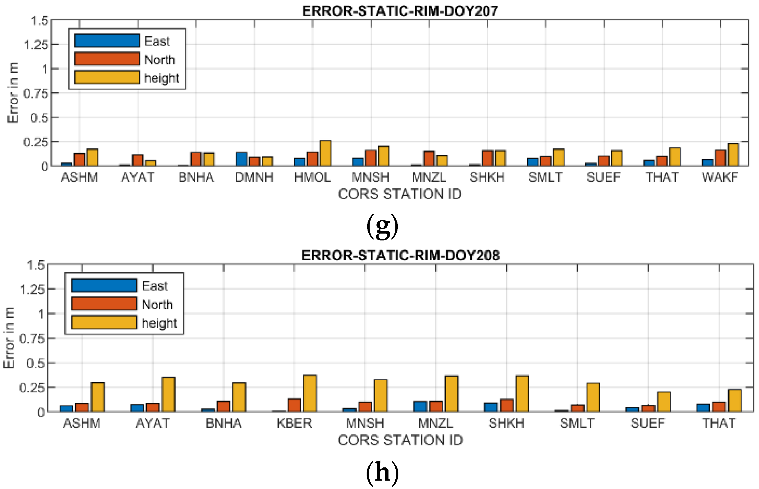
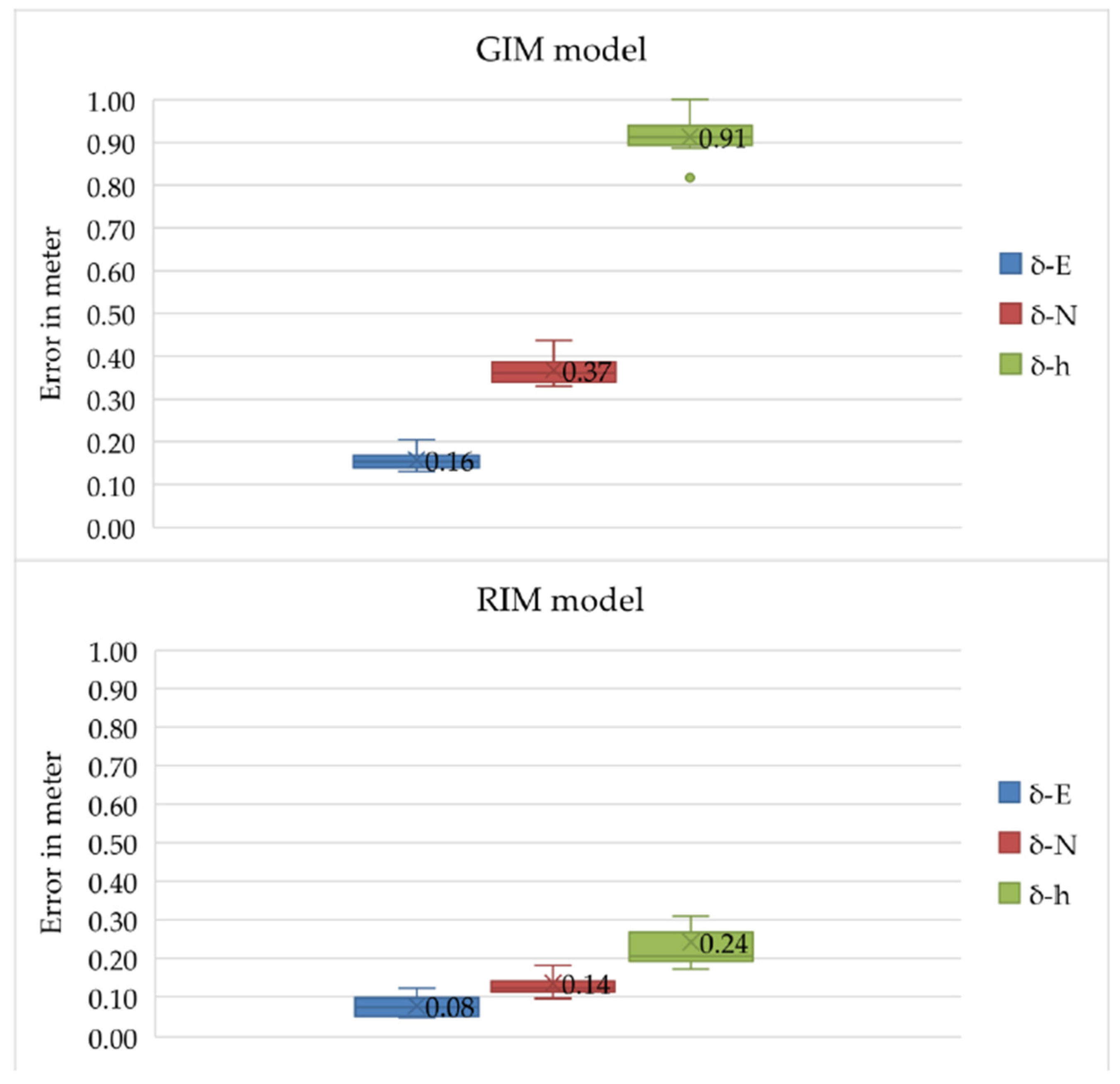
5.1. Statistical Analysis

The errors (δ) for the horizontal components (East and North) and height between the reference network and PPP solutions were determined to evaluate the SF-PPP solution using the two ionosphere models. As shown in Figure 6, the error values for each observation day are presented for the GIM model solution. The horizontal axis refers to the station ID and the vertical one presents the errors in meters. For all observation days and all stations, the findings for the east direction indicate an error range of 0.006–0.45 m with an average value of 0.15 m. It can be seen that DOY 202 reported the least errors, while DOY 203 reported the greatest errors due to some data quality problems; more details about the data quality are explained in ref. [36]. This may include factors such as differences in solar activity and ionospheric conditions. However, the solution shows an average value of 0.15 m. The error increases for the north direction, whereas the figure shows that the error differs for all observation days from 0.16–0.59 m (Average = 0.36 m). A significant ionosphere effect is reported for the height component; the error states an average value of less than 1 m.
Figure 7 shows the obtained static SF-PPP solution using the developed Egyptian ionosphere regional model. According to the study, the best solution is in the East, followed by the North and height, respectively. For all observation days, the East component shows an error range of up to 0.14 m; only DOY 201 and 203 report a higher error range of up to 0.32 m. Further, the whole solution indicates 0.07 m as an average value. The result provides an error range of 0.06–0.28 m with an average of 0.13 m in the North direction. The highest error is obtained from the height component, where the error measures between 0.26 and 0.46 m; only station WAKF in DOY 201 shows a high value of 0.76 m due to the lack of observation data for 22 h, which means that only 2 h were processed. However, the average value is 0.24 m.

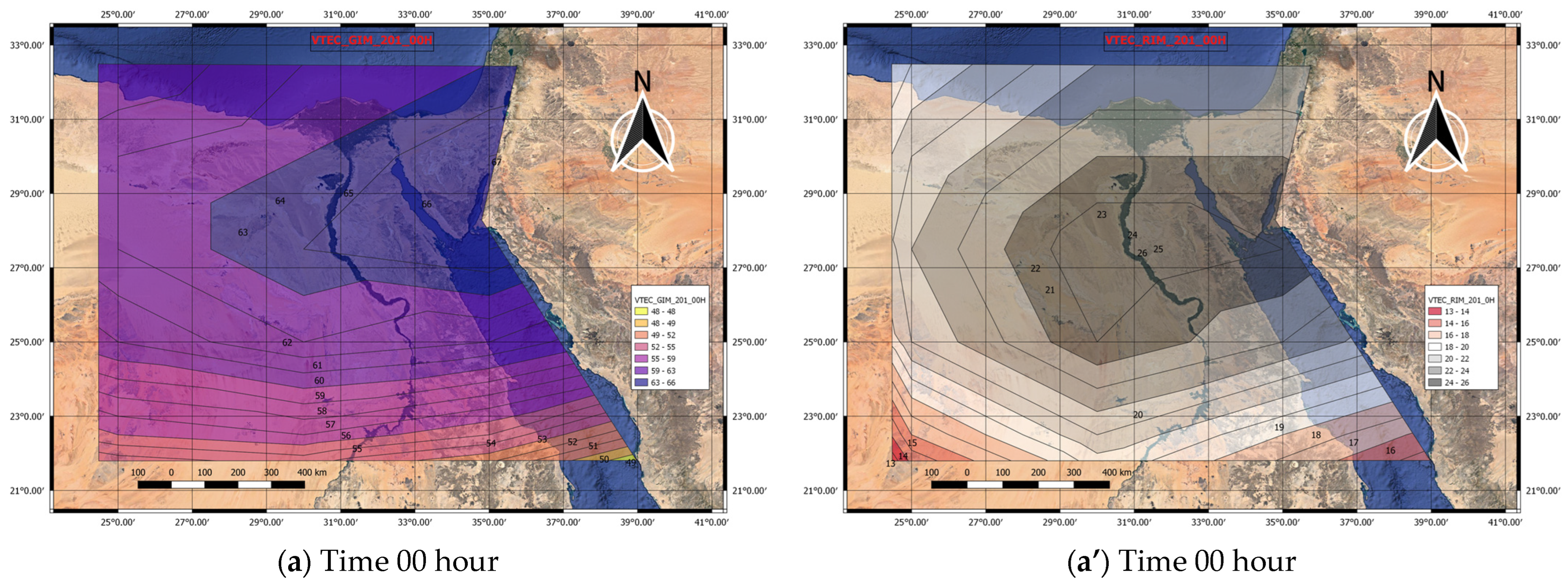
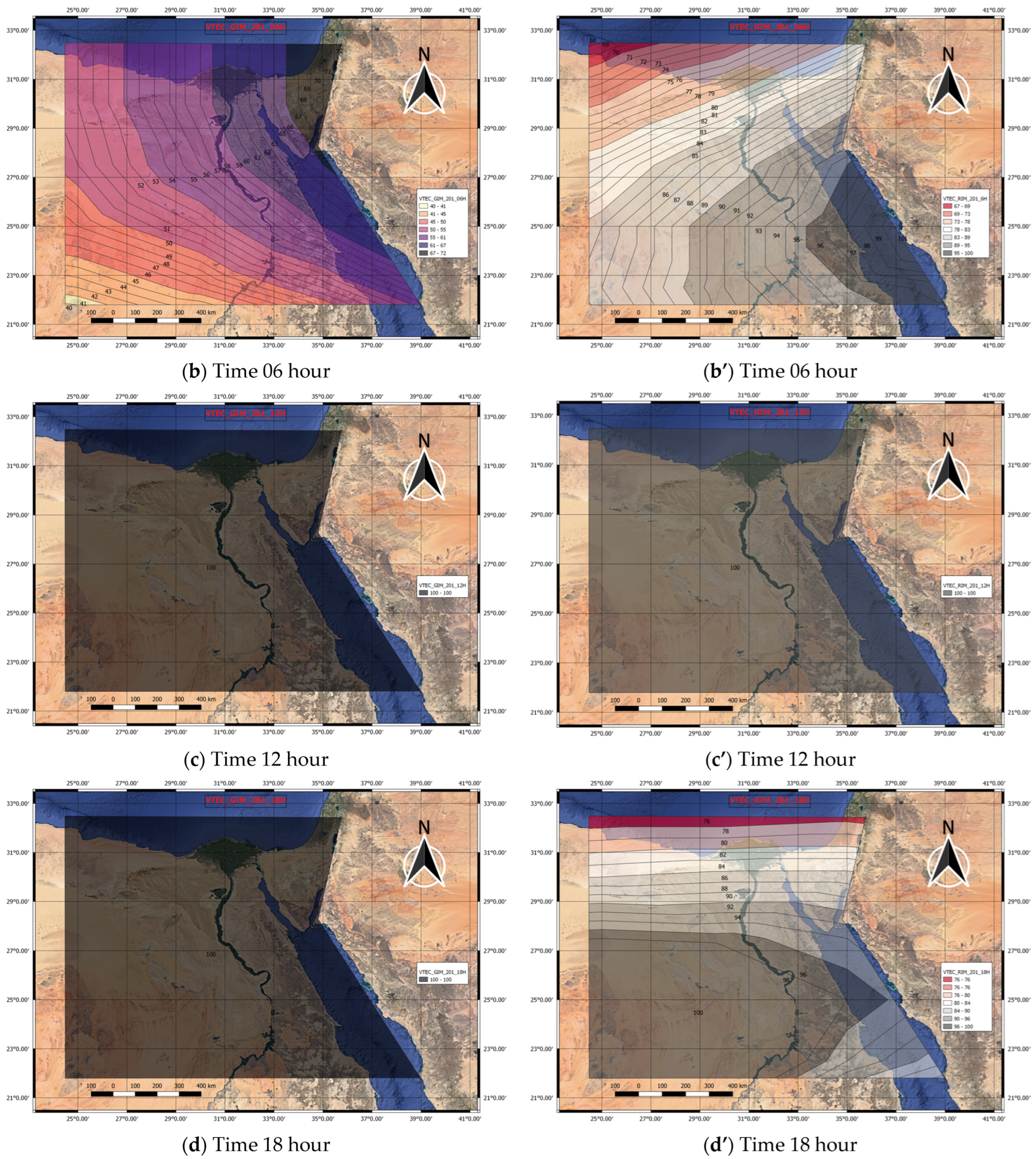
5.2. Graphical Analysis

A Matlab code was developed to extract the VTEC values related to the longitude and latitude over Egypt to visualize the ionosphere maps from GIM maps and then model them using the regional CORS stations. This Matlab code reads the ionosphere maps in IONEX format that is provided by GIM-CODE and the one estimated regional model (RIM). After that, the obtained files in Excel format are input into QGIS software to be visualized as explained in Figure 8. Figure 8 shows an example of the ionosphere maps for GIM, and the developed RIM model for DOY 201. The figure presents the ionosphere maps as contour maps over Egypt. The left figures refer to the GIM model; moreover, the right ones mention the RIM model. At midnight, the GIM model shows a VTEC value of 48–66, while the RIM model presents a VTEC value between 13–26. The highest values for both models are represented over Sinai, from middle to South Egypt to the western desert. At 6:00 A.M., the GIM model presents VTEC values of 40–72 decreased in the South-West direction. In addition, the RIM model shows values of 68–100 decreased in the North-West direction. In the afternoon, the two models present a high VTEC value (100). At 6:00 P.M., the GIM model still indicates a high level in the other directions, while the RIM model represents high values in the South and decreases towards the North.

6. Discussion

Table 4 below illustrates detailed statistics for the SF-PPP solution using GIM mode. This table displays the data for each CORS station in the East, North, and height in addition to the minimum (min.), maximum (max.), average (avg.), and standard deviation (SD) of error. It is apparent from this table that in the East direction, most of the stations report an average error of 0.13–0.17 m; only three stations show higher values. MNSH shows 0.18 m; stations KBER and WAKF also show 0.20 m. Regarding the SD that refers to the precision, the solution shows a range of 0.07–0.10 m; only four stations (ISNA, KBER, MNHS, and WAKF) report less precision. The North component of the error is higher than the East direction. The result shows an average error of 0.33–0.44 m for all stations. The solution has variant SD values; most stations have a SD of 0.02–0.07 m. Conversely, stations BADR, DMNH, HMOL, ISAN, KBER, and MNSH represent a SD value of 0.17–0.21 m. From the data in this table, the error in the height direction is the most obvious; the obtained errors show an average value of 0.82–0.94 m. The solution indicates that the SD values are in the range of 0.09–0.17 m; only the same six stations mentioned in the north direction report a SD of 0.35–0.50 m.
Regarding the SF-PPP solution obtained from the RIM model, Table 5 shows the statistics values for each CORS station during the observation days. For all stations, the error in the East direction ranges from 0.05 to 0.08 m on average. Only the stations BADR, ISNA, KBER, and WAKF have an average error of 0.1–0.12 m. However, the solution in the East direction shows a SD of 0.06 for all stations. The ISNA station has the highest average error of 0.24 m in the North direction, whereas the other stations only provide an error of 0.13 m (SD = 0.04 m). Regarding the height component, three stations (ISNA, MNSH, and WAKF) report a high error of 0.31–0.40 m. The other stations indicate a lower average error of 0.21 m. Overall, the height solution has a SD of 0.11 m.
The reasons for the variations in the accuracy of SF-PPP for CORS stations are discussed below. Table 6 displays the observation times of the stations with low accuracy for the RIM model’s SF-PPP solution. For example, for DOY 201, station WAKF has an observation time of 1.30 h, while for DOY 202, 204, 205, and 206, it has an observation time of less than 24 h. These losses additionally decrease the final SF-PPP solution’s accuracy.
Figure 9 concludes the box plot average errors for the SF-PPP solution obtained by using the GIM-CODE and RIM models. The upper figure refers to the SF-PPP solution from the CODE-GIM model; the lower plot refers to the SF-PPP solution from the RIM model. Box plots are graphical representations of data that show the median, quartiles, and outliers of a dataset. The range of values that falls between the first and third quartiles of the data is denoted by the interquartile range (IQR), which is depicted by the box. Outliers are depicted as individual points that lie beyond the whiskers and extend from the box to the highest and lowest values that fall within 1.5 times the IQR. In our work, the box plot of errors for the new Regional Ionosphere Model (RIM) has a narrow box and small whiskers compared to the box plot of errors for the Global Ionosphere Model (GIM). This shows that the RIM model is more reliable and has less variation in how well it works than the GIM model. The median error for the RIM model is also less than the median error for the GIM model. This means that the RIM model performs better overall.

7. Conclusions

The present study presents a new method to develop a new regional ionosphere model (RIM) for Egypt. This regional model was developed using 18 CORS stations that cover the whole of Egypt. The determined model has a temporal resolution of 2 h and a spatial resolution of 2.5° × 5° for latitude and longitude. The RIM model was derived from the code phase geometry-free linear combination (P4) using Bernese GNSS V. 5.2 software. The static SF-PPP results were estimated using Bernese GNSS V. 5.2 software. Two solutions were obtained: one using the GIM model, and the other using the RIM model. The regional model’s SF-PPP solution produced an average error of 0.06 m in the eastern direction, 0.13 m in the northern direction, and 0.21 m in the vertical dimension. This solution is better than the solution using the GIM model with a percentage of 60%, 68%, and 77% in East, North, and height, respectively.

Author Contributions

Conceptualization, A.A., T.A. and V.S.; Methodology, A.A. and V.S.; Software, A.A. and V.S.; Validation, A.A.; Formal analysis, A.A. and V.S.; Investigation, A.A.; Resources, T.A. and V.S.; Writing—original draft, A.A. and T.A.; Writing—review & editing, A.A. and V.S.; Visualization, A.A.; Supervision, V.S.; Funding acquisition, V.S. All authors have read and agreed to the published version of the manuscript.

Funding

This research received no external funding.

Data Availability Statement

Not applicable.

Conflicts of Interest

The authors declare no conflict of interest.

References

  1. Seeber, G. Satellite Geodesy, 2nd ed.; Walter de Gruyter: Berlin, Germany, 2003. [Google Scholar]
  2. Misra, P.; Enge, P. Global Positioning System: Signals, Measurements, and Performance, 2nd ed.; Ganga-Jumana Press: Lincoln, MA, USA, 2012. [Google Scholar]
  3. Klobuchar, J.A. Ionospheric time-delay algorithm for single-frequency GPS users. IEEE Trans. Aerosp. Electron. Syst. 1987, 3, 325–331. [Google Scholar] [CrossRef]
  4. Schaer, S.; Gurtner, W.; Feltens, J. IONEX: The ionosphere map exchange format version 1. In Proceedings of the IGS AC Workshop, Darmstadt, Germany, 9–11 February 1998. [Google Scholar]
  5. IONEX. Ionosphere Products. Available online: https://cddis.nasa.gov/archive/gnss/products/ionex/yyyy/ddd (accessed on 20 April 2023).
  6. Hernández-Pajares, M.; Juan, J.M.; Sanz, J.; Orus, R.; Garcia-Rigo, A.; Feltens, J.; Komjathy, A.; Schaer, S.C.; Krankowski, A. The IGS VTEC maps: A reliable source of ionospheric information since 1998. J. Geod. 2009, 83, 263–275. [Google Scholar] [CrossRef]
  7. Bilitza, D.; Rawer, K.; Bossy, L.; Gulyaeva, T. International reference ionosphere—Past, present, and future: I. Electron density. Adv. Space Res. 1993, 13, 3–13. [Google Scholar] [CrossRef]
  8. Radicella, S.M.; Zhang, M.-L. The improved DGR analytical model of electron density height profile and total electron content in the ionosphere. Ann. Geophys. 1995, 1, 35–41. [Google Scholar] [CrossRef]
  9. Hochegger, G.; Nava, B.; Radicella, S.; Leitinger, R. A family of ionospheric models for different uses. Phys. Chem. Earth Part C Sol. Terr. Planet. Sci. 2000, 25, 307–310. [Google Scholar] [CrossRef]
  10. Radicella, S.M. The NeQuick model genesis, uses and evolution. Ann. Geophys. 2009, 52, 417–422. [Google Scholar]
  11. Bhuyan, P.; Borah, R.R. TEC derived from GPS network in India and comparison with the IRI. Adv. Space Res. 2007, 39, 830–840. [Google Scholar] [CrossRef]
  12. Opperman, B.D.; Cilliers, P.J.; McKinnell, L.A.; Haggard, R. Development of a regional GPS-based ionospheric TEC model for South Africa. Adv. Space Res. 2007, 39, 808–815. [Google Scholar] [CrossRef]
  13. Başçiftçi, F.; Cevat, I.N.A.L.; Yildirim, O.; Bulbul, S. Comparison of regional and global TEC values: Turkey model. Int. J. Eng. Geosci. 2018, 3, 61–72. [Google Scholar] [CrossRef]
  14. Tu, R.; Zhang, H.; Ge, M.; Huang, G. A real-time ionospheric model based on GNSS Precise Point Positioning. Adv. Space Res. 2013, 52, 1125–1134. [Google Scholar] [CrossRef]
  15. Durmaz, M.; Karslioglu, M.O. Regional vertical total electron content (VTEC) modeling together with satellite and receiver differential code biases (DCBs) using semi-parametric multivariate adaptive regression B-splines (SP-BMARS). J. Geod. 2015, 89, 347–360. [Google Scholar] [CrossRef]
  16. Hoque, M.; Jakowski, N. An alternative ionospheric correction model for global navigation satellite systems. J. Geod. 2015, 89, 391–406. [Google Scholar]
  17. Kao, S.P.; Chen, Y.C.; Ning, F.S.; Tu, Y.M. An LS-MARS method for modeling regional 3D ionospheric electron density based on GPS data and IRI. Adv. Space Res. 2015, 55, 2256–2267. [Google Scholar] [CrossRef]
  18. Rovira-Garcia, A.; Juan, J.M.; Sanz, J.; Gonzalez-Casado, G. A worldwide ionospheric model for fast precise point positioning. IEEE Trans. Geosci. Remote Sens. 2015, 53, 4596–4604. [Google Scholar] [CrossRef] [Green Version]
  19. Xi, G.; Zhu, F.; Gan, Y.; Jin, B. Research on the regional short-term ionospheric delay modeling and forecasting methodology for mid-latitude area. GPS Solut. 2015, 19, 457–465. [Google Scholar] [CrossRef]
  20. Abdelazeem, M.; Çelik, R.N.; El-Rabbany, A. An improved regional ionospheric model for single-frequency GNSS users. Surv. Rev. 2017, 49, 153–159. [Google Scholar]
  21. Abdelazeem, M.; Çelik, R.N.; El-Rabbany, A. An enhanced real-time regional ionospheric model using IGS real-time service (IGS-RTS) products. J. Navig. 2016, 69, 521–530. [Google Scholar] [CrossRef] [Green Version]
  22. Dach, R.; Schaer, S.; Arnold, D.; Orliac, E.; Prange, L.; Susnik, A.; Villiger, A.; Jäggi, A. CODE Final Product Series for the IGS. 2016. Available online: https://boris.unibe.ch/75876/1/AIUB_AFTP.TXT (accessed on 27 April 2023).
  23. Li, M.; Lei, Z.; Li, W.; Jiang, K.; Huang, T.; Zheng, J.; Zhao, Q. Performance Evaluation of Single-Frequency Precise Point Positioning and Its Use in the Android Smartphone. Remote Sens. 2021, 13, 4894. [Google Scholar] [CrossRef]
  24. Li, W.; Yuan, K.; Odolinski, R.; Zhang, S. Regional Ionospheric Maps with Quad-Constellation Raw Observations as Applied to Single-Frequency PPP. Remote Sens. 2022, 14, 6149. [Google Scholar] [CrossRef]
  25. Tawfeek, H.; Sedeek, A.; Rabah, M.; El-Fiky, G. Regional Ionosphere Mapping Using Zero Difference GPS Carrier Phase. Ann. Geophys. Discuss. 2018, 1–16. [Google Scholar] [CrossRef]
  26. Sedeek, A. Ionosphere delay remote sensing during geomagnetic storms over Egypt using GPS phase observations. Arab. J. Geosci. 2020, 13, 811. [Google Scholar] [CrossRef]
  27. Elghazouly, A.A.; Doma, M.I.; Sedeek, A.A. Validating the impact of various ionosphere correction on mid to long baselines and point positioning using GPS dual-frequency receivers. J. Appl. Geod. 2022, 16, 81–90. [Google Scholar] [CrossRef]
  28. Abdallah, A.; Agag, T.; Schwieger, V. Validation of CODE-GIM and Regional Ionosphere Model (RIM) for Single Frequency GNSS PPP Solution using Bernese GNSS software-Case Study: Egyptian Nile Delta. FIG Peer Rev. J. 2022. Available online: https://www.researchgate.net/publication/362208479_Validation_of_CODE-GIM_and_Regional_Ionosphere_Model_RIM_for_Single_Frequency_GNSS_PPP_Solution_using_Bernese_GNSS_software_-Case_Study_Egyptian_Nile_Delta (accessed on 27 April 2023).
  29. IGS. International GNSS Service (IGS). Available online: https://igs.org/station-resources/ (accessed on 6 November 2022).
  30. Teunissen, P.J.G.; Kleusberg, A. GPS Observation Equations and Positioning Concepts. In GPS for Geodesy; Teunissen, P.J.G., Kleusberg, A., Eds.; Springer: Berlin/Heidelberg, Germany, 2007; pp. 175–217. [Google Scholar]
  31. Dach, R.; Lutz, S.; Walser, P.; Fridez, P. Bernese GNSS Software, Version 5.2; AIUB-Astronomical Institute, University of Bern: Bern, Switzerland, 2015.
  32. Schaer, S. Mapping and Predicting the Earth’s Ionosphere Using the Global Positioning System. Ph. D. Thesis, Bern University, Bern, Switzerland, 1999. [Google Scholar]
  33. Schaer, S.; Beutler, G.; Mervart, L.; Rothacher, M.; Wild, U. Global and regional ionosphere models using the GPS double difference phase observable. In Proceedings of the IGS Workshop” Special Topics and New Directions”, Potsdam, Germany, 15–17 May 1995. [Google Scholar]
  34. Abdallah, A. Precise Point Positioning for Kinematic Applications to Improve Hydrographic Survey. Ph.D. Dissertation, University of Stuttgart, Stuttgart, Germany, 2016. [Google Scholar]
  35. TBC. Trimble Business Center (TBC) Software. Available online: https://geospatial.trimble.com/products-and-solutions/trimble-business-center (accessed on 14 December 2022).
  36. Abdallah, A.; Agag, T. Reliability of CSRS-PPP for Validating the Egyptian Geodetic Cors Networks. Artif. Satell. 2022, 57, 58–76. [Google Scholar] [CrossRef]
  37. Abdallah, A.; Agag, T.; Dawod, G. ITRF-Based Tectonic Coordinates Changes using GNSS-CORS Networks: A Case Study of Egypt. Surv. Land Inf. Sci. 2021, 80, 69–78. [Google Scholar]
Figure 1. IGS Stations, last updated 2019 [29]. The black box indicates that there are poor coverage of the IGS stations in North Africa.
Remotesensing 15 03147 g001
Figure 2. Single-layer model based on [31].
Remotesensing 15 03147 g002
Figure 3. Process flow diagram using Bernese GNSS software.
Remotesensing 15 03147 g003
Figure 4. CORS stations for reference solution according to the Google Earth platform.
Remotesensing 15 03147 g004
Figure 5. Egy. SA-CORS station layout according to the Google Earth platform.
Remotesensing 15 03147 g005
Figure 6. Errors in SF-PPP using the CODE-GIM model. (a) DOY 201. (b) DOY 202. (c) DOY 203. (d) DOY 204. (e) DOY 205. (f) DOY 206. (g) DOY 207. (h) DOY 208.
Remotesensing 15 03147 g006aRemotesensing 15 03147 g006b
Figure 7. Errors in SF-PPP using the RIM model. (a) DOY 201. (b) DOY 202. (c) DOY 203. (d) DOY 204. (e) DOY 205. (f) DOY 206. (g) DOY 207. (h) DOY 208.
Remotesensing 15 03147 g007aRemotesensing 15 03147 g007b
Figure 8. Ionosphere maps for CODE-GIM and RIM models; the left figures refer to the CODE-GIM model, and the right figures refer to RIM figures.
Remotesensing 15 03147 g008aRemotesensing 15 03147 g008b
Figure 9. Box plot of the average error values of SF-PPP solution; the upper figure refers to the CODE-GIM model, and the lower figure refers to RIM figures.
Remotesensing 15 03147 g009
Table 1. Downloaded files from FTP server.
File IDDescription
CODwwwwd.CLKIt refers to the satellite’s precise clocks with an interval of 30 s
CODwwwwd.EPHIt mentions the satellite’s precise orbits (.SP3)
CODwwwwd.ERP & CODwwww7.ERPIt refers to the daily and weekly earth rotation parameters
CODwwwwd.IONIt denotes the CODE’s global ionosphere maps
CODyymm.DCBIt indicates the CODE’s monthly solution for GPS P1-C1 and P1-P2 code biases for satellites and receivers in the format [yy: year, mm: month]
PCV_COD.I14It presents the list of antenna phase center variations derived from the ANTEX file in the format [I14.ATX]
CONSTIt lists the general constants used during processing
DATUMIt contains a list of datum definitions for the software
RECEIVERIt identifies a list of receiver information files for the software
SAT_yyyy.CRXIt defines a list of satellite problems
SATELLITE.I14It summarizes a list of satellite-specific information
TIDE2000.TPO, IAU2000R06.NUT, IERS2010XY.SUB, and OT_FES2004.TIDThese files refer to the coefficients for the solid earth tide, nutation, sub-daily pole, and ocean tide models, respectively.
Table 2. RIM’s parameters.
ParameterValue
Satellite constellationGPS/GLONASS
ObservationZero-Difference
Frequency combinationP4
Cutoff elevation angle10°
Sampling interval30 s
Temporal resolution2 h
Nmax: max. degree of spherical harmonics6
Mmax: max. order of spherical harmonics6
H: height of single layer450 km
Reference frame definitionGeomagnetic
Geomagnetic pole (Latitude)79°
Geomagnetic pole (Longitude)−71°
Grid (Lat. × Long.)2.5° × 5°
Table 3. Availability of Rinex data for validation stations. (✔) means the Rinex data is available; (x) means the Rinex data is not available.
NO.STATION IDDOY
201
DOY
202
DOY
203
DOY
204
DOY
205
DOY
206
DOY
207
DOY
208
1ASHM
2AYAT
3BADRxx
4BNHA
5DMNHx
6HMOLx
7ISNAxx
8KBERxxx
9MNSHxx
10MNZL
11SHKH
12SMLT
13SUEF
14THAT
15WAKFx
Table 4. GIM statistics.
EASTNORTHHEIGHT
Min.Max.Avg.SDMin.Max.Avg.SDMin.Max.Avg.SD
ASHM0.060.300.160.070.260.410.350.050.681.140.920.13
AYAT0.060.310.170.080.290.420.360.050.721.080.890.13
BADR0.080.270.160.090.270.590.390.200.171.010.820.47
BNHA0.050.260.140.070.220.410.340.060.721.020.900.10
DMNH0.020.260.140.100.160.470.380.170.641.090.910.35
HMOL0.040.260.140.080.300.430.350.130.711.020.890.33
ISNA0.010.400.130.130.380.540.440.210.711.020.900.43
KBER0.050.440.200.150.300.450.390.210.841.090.930.50
MNSH0.090.380.180.120.320.490.390.150.681.180.890.35
MNZL0.050.270.150.070.270.400.340.050.731.280.940.17
SHKH0.070.250.160.070.280.390.340.040.721.170.900.15
SMLT0.020.250.150.070.300.360.330.020.771.080.940.09
SUEF0.020.280.130.080.240.400.350.050.721.110.920.11
THAT0.040.320.150.080.300.460.400.060.711.090.940.14
WAKF0.060.450.200.140.300.520.390.070.761.301.000.16
Table 5. RIM statistics.
EASTNORTHHEIGHT
Min.Max.Avg.SDMin.Max.Avg.SDMin.Max.Avg.SD
ASHM0.000.180.050.050.080.130.100.020.050.300.180.08
AYAT0.000.230.080.080.090.150.120.020.050.380.250.11
BADR0.010.210.100.080.080.240.120.080.110.410.260.15
BNHA0.000.160.050.050.090.140.110.020.110.290.190.07
DMNH0.020.160.070.060.090.190.140.060.030.380.190.14
HMOL0.030.170.070.050.100.150.130.050.080.330.190.11
ISNA0.010.290.100.100.210.280.240.110.340.470.400.19
KBER0.030.320.110.110.100.150.130.070.070.280.170.11
MNSH0.010.280.090.090.130.200.170.060.200.460.310.14
MNZL0.010.140.050.040.070.150.120.030.080.440.200.13
SHKH0.010.150.060.050.090.160.120.020.040.360.200.11
SMLT0.010.110.070.030.080.130.110.020.140.370.230.08
SUEF0.010.170.050.050.070.110.100.010.110.320.210.09
THAT0.040.220.080.060.060.180.140.040.180.440.270.09
WAKF0.020.320.120.110.080.130.100.020.230.760.390.17
Table 6. Observation time of some Egy. SA-CORS stations.
DOYStation IDObservation
Time (Hours)
DOYStation IDObservation
Time (Hours)
201MNSH13.25204ISNA17.48
MNZL15.70THAT22.23
WAKF1.30WAKF16.52
202ISNA20.87205ISNA20.00
WAKF17.78WAKF16.80
203ISNA20.93206ISNA16.77
KBER7.5WAKF17.05
MNSH21.2
Disclaimer/Publisher’s Note: The statements, opinions and data contained in all publications are solely those of the individual author(s) and contributor(s) and not of MDPI and/or the editor(s). MDPI and/or the editor(s) disclaim responsibility for any injury to people or property resulting from any ideas, methods, instructions or products referred to in the content.

