Characterization and Analysis of Landslide Evolution in Intramountain Areas in Loja (Ecuador) Using RPAS Photogrammetric Products

Abstract

This case study focuses on the area of El Plateado near the city of Loja, Ecuador, where landslides with a high impact on infrastructures require monitoring and control. The main objectives of this work are the characterization of the landslide and the monitoring of its kinematics. Four flights were conducted using a remotely piloted aerial vehicle (RPAS) to capture aerial images that were processed with SfM techniques to generate digital elevation models (DEMs) and orthoimages of high resolution (0.05 m) and sufficient accuracy (below 0.05 m) for subsequent analyses. Thus, the DEM of differences (DoD) and profiles are obtained, but a morphometric analysis is conducted to quantitatively characterize the landslide’s elements and study its evolution. Parameters such as slope, aspect, topographic position index (TPI), terrain roughness index (TRI), and topographic wetness index (TWI) are analyzed. The results show a higher slope and roughness for scarps compared to stable areas and other elements. From TPI, slope break lines have been extracted, which allow the identification of landslide features such as scarps and toe tip. The landslide shows important changes in the landslide body surface, the retraction of the main scarp, and advances of the foot. A general decrease in average slope and TRI and an increase in TWI are also observed due to the landslide evolution and stabilization. The presence of fissures and the infiltration of rainfall water in the unsaturated soil layers, which consist of high-plasticity clays and silts, contribute to the instability. Thus, the study provides insights into the measurement accuracy, identification and characterization of landslide elements, morphometric analysis, landslide evolution, and the relationship with geotechnical factors that contribute to a better understanding of landslides. A higher frequency of the RPAS surveys and quality of geotechnical and meteorological data are required to improve the instability analysis together with a major automation of the GIS procedures.

1. Introduction

The study of landslides is of vital importance to understand and mitigate the risks associated with natural phenomena as well as to promote the sustainable development of affected areas. Understanding the characterization and analysis of the evolution of landslides plays a fundamental role in the Sustainable Development Goals, because it allows an adequate management of natural resources, more efficient territorial planning, and protection of the communities that inhabit areas prone to landslides [1,2,3,4]. Understanding the characterization and analysis of landslide evolution can significantly contribute to the Sustainable Development Goals in several ways:

Disaster risk management: Understanding the characterization of landslides and their evolution makes it possible to identify landslide-prone areas and assess the associated risk. This facilitates the implementation of adequate prevention and mitigation measures to reduce the exposure of communities to landslides [5,6]. By minimizing the risks of natural disasters, both people and the natural environment are protected, contributing to long-term sustainability.

Sustainable urban planning: Analysis of the evolution of landslides helps to understand how human activities can contribute to their occurrence. This is especially relevant in the context of urban planning, where the growth of cities can increase the pressure on slopes and unstable terrain [7,8]. By taking this information into account, regulations and development guidelines can be established to avoid construction in areas of high landslide risk, thus promoting more sustainable urban planning.

Ecosystem conservation: Landslides can have a significant impact on ecosystems, altering soils, vegetation, and local hydrology. Understanding the characterization of landslides and their evolution makes it possible to identify the factors that contribute to their appearance, such as deforestation or soil degradation [9]. By taking steps to preserve and restore natural ecosystems, you can strengthen the resilience of vulnerable areas to landslides and promote environmental sustainability.

Natural resource management: Landslides can impact the availability and quality of natural resources such as water and fertile soil. Through the characterization and analysis of landslides, it is possible to understand how these processes affect natural resources and take measures for their sustainable management. For example, soil and water conservation practices can be implemented to reduce erosion and prevent landslides, thus ensuring the availability of essential resources for future generations. To study natural hazards, specifically landslides, it is necessary to have techniques and procedures that provide information on terrain evolution with sufficient spatial and temporal resolution [10,11,12,13,14,15] to determine geomorphic changes. Currently, Global Navigation Satellite Systems (GNSS) [16,17,18,19,20] and Terrestrial Laser Scanning (TLS) are commonly used, which provide high-density point clouds and high-quality digital elevation models [21]. However, these techniques require significant processing time and are costly. In this context, the use of remotely piloted aerial systems (RPAS), also known as drones, represents a low-cost alternative [22,23,24] that enables the acquisition of high-resolution aerial imagery for mapping and monitoring small-scale areas [5,25,26,27].

The use of RPAS in the study of landslides has allowed for the evaluation of their kinematic behavior and temporal evolution [5,25,26,28,29,30]. This is achieved through the acquisition of photogrammetric products derived from precise processing, enabling measurements that can even detect small-scale terrain changes. Structure from Motion (SfM) algorithms are employed for images orientation [31,32,33,34] providing accuracies of about 0.10 m from which photogrammetric products such as DEMs and orthoimages are obtained. The former are usually compared by means of DEM of differences (DoDs) and the latter are used for interpretation and digital image correlation (DIC) [25,26,27,35,36,37,38,39,40,41,42,43,44,45]. The accuracy of photogrammetric products largely depends on the number and distribution of ground control points (GCPs) and checkpoints (CHK) measured using GNSS techniques [16,25,38,46,47], which enable model orientation [17]. Additionally, geodetic measurements [45] using GNSS techniques provide high-precision coordinate estimation, making them valuable for monitoring surfaces undergoing both slow and rapid deformations at different scales [48].

The geomorphometric approach [49] is employed to analyze the morphology of the terrain based on high-resolution digital elevation models (DEMs) derived from LiDAR systems or through RPAS photogrammetry, which allows for the detection of subtle changes in the topography. This information can be used to generate maps of slope, aspect, curvature and roughness, among others, which help to characterize landslides, identify their elements, and understand the kinematics and dynamics of the slope [50,51,52,53,54].

Recent findings regarding landslides in Ecuador have significant implications for the understanding and management of this natural phenomenon. These discoveries allowed for a greater understanding of the determinant and triggering factors of landslides, such as topography, geology, seismic activity, and weather conditions. In addition, they have made it possible to identify areas prone to this type of event [55,56], which contributes to better urban and rural planning, as well as the implementation of preventive and adequate mitigation measures. These findings have also improved the ability to monitor land changes in landslides areas based on classical approaches such as photointerpretation, DoDs calculation and point extraction and measurement [57], which is essential to alert communities at risk and take timely measures to ensure the safety of the population. However, other approaches are required such as DIC for a better measurement of displacements; object-based analysis (OBIA) for features identification; and morphometric analysis, the approach implemented in this work, for landslide and terrain characterization. In general, scientific advances in this field are strengthening Ecuador’s resilience against landslides and require a solid foundation for the development of effective natural risk management strategies.

Thus, the main objectives of this study are: (a) the characterization of the landslide, identifying its elements and describing its morphology; and (b) the monitoring of its kinematics. For it, we have analyzed not only the direct photogrammetric products such as DEM and orthoimages but also topographic or morphometric parameters and their changes. The detailed and systematic analysis of these parameters is the main contribution of this study, which has allowed precise landslide characterization and monitoring. Previous works have focused on some parameters such as slope [52,53], aspect [53], curvature [51,52,53,54], roughness [50,53] or TWI [50], but none have examined all of them and even less with a multitemporal approach that allows landslide monitoring.

Thus, multitemporal RPAS flights were captured in a landslide in the El Plateado sector of the city of Loja, Ecuador. One of the main advantages of RPAS is their capability to fly at altitudes below 100 m, allowing for the integration of new sensors on aerial platforms. RPAS can capture images from various angles, provide flexibility in conducting work at different scales, offer cost-effective solutions, and deliver high-quality results [15,16,17,18]. RPAS technology has been successfully used for the cartography and monitoring of areas spanning few square kilometers.

The scheduled flights allowed for the acquisition of images, which once processed, produced orthoimages and DEMs. For this purpose, the photogrammetric image blocks were oriented using SfM techniques with the support of ground control points whose positions were determined using differential GNSS. The interpretation of the orthoimages has allowed the observation of morphological features and changes in land cover and elements affected by the landslide. Moreover, from DEMs, longitudinal profiles, DEMs of differences (DoDs), and especially detailed maps of morphometric parameters derived from DEMs such as slope, aspect, TPI, TRI, and TWI were obtained. These models have enabled the detection of morphologies that contribute to the characterization of landslides in the study area, and furthermore, due to their multitemporal nature, the analysis of their temporal evolution.

2. Materials and Methods

2.1. Study Area

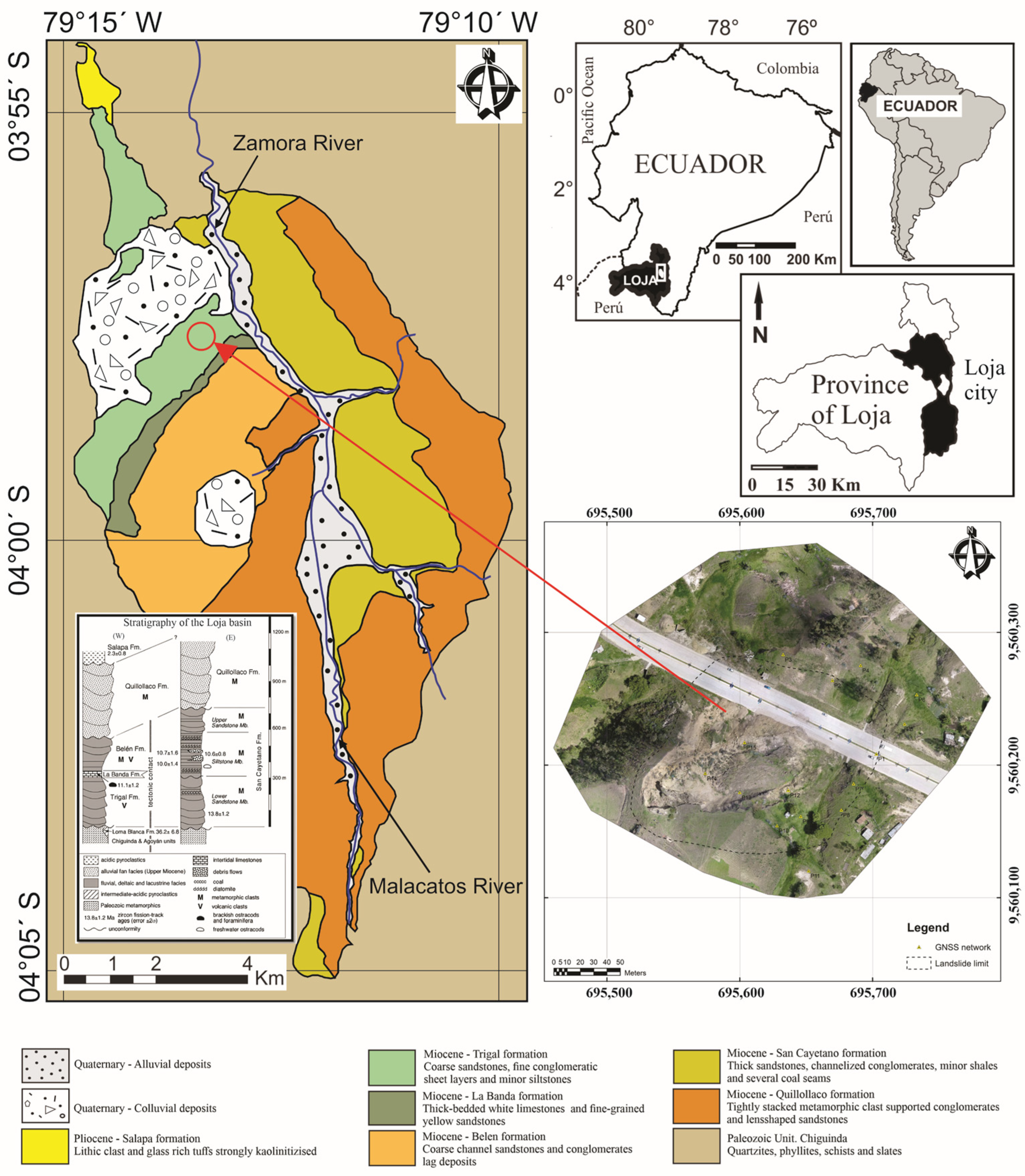
The study area is situated in the El Plateado sector on the western side of the city of Loja, located in southern Ecuador, along the bypass road (Figure 1). Geologically, the study area is part of the Trigal Formation (Miocene), which is primarily exposed in the western portion of the basin (Figure 1). It predominantly consists of a homogeneous, finely laminated brown clay with occasional gypsum veins. Additionally, it comprises coarse-grained sandstones with thin layers of conglomerate and minor occurrences of limonite. The sandstones exhibit horizontal stratification with crossbedding planes.

The activity of the landslide is evident through the deposition of material at the low part of the hillslope as well as the presence of cracks, lobes, and the formation of main, lateral, and secondary scarps resulting from the ongoing movement and material detachment (Figure 2b–d). The progressive development of the main scarp and the right (southern) flank of the landslide caused the collapse of a residential structure (Figure 2a) without any reported loss of human life.

2.2. Materials (RPAS and GNSS)

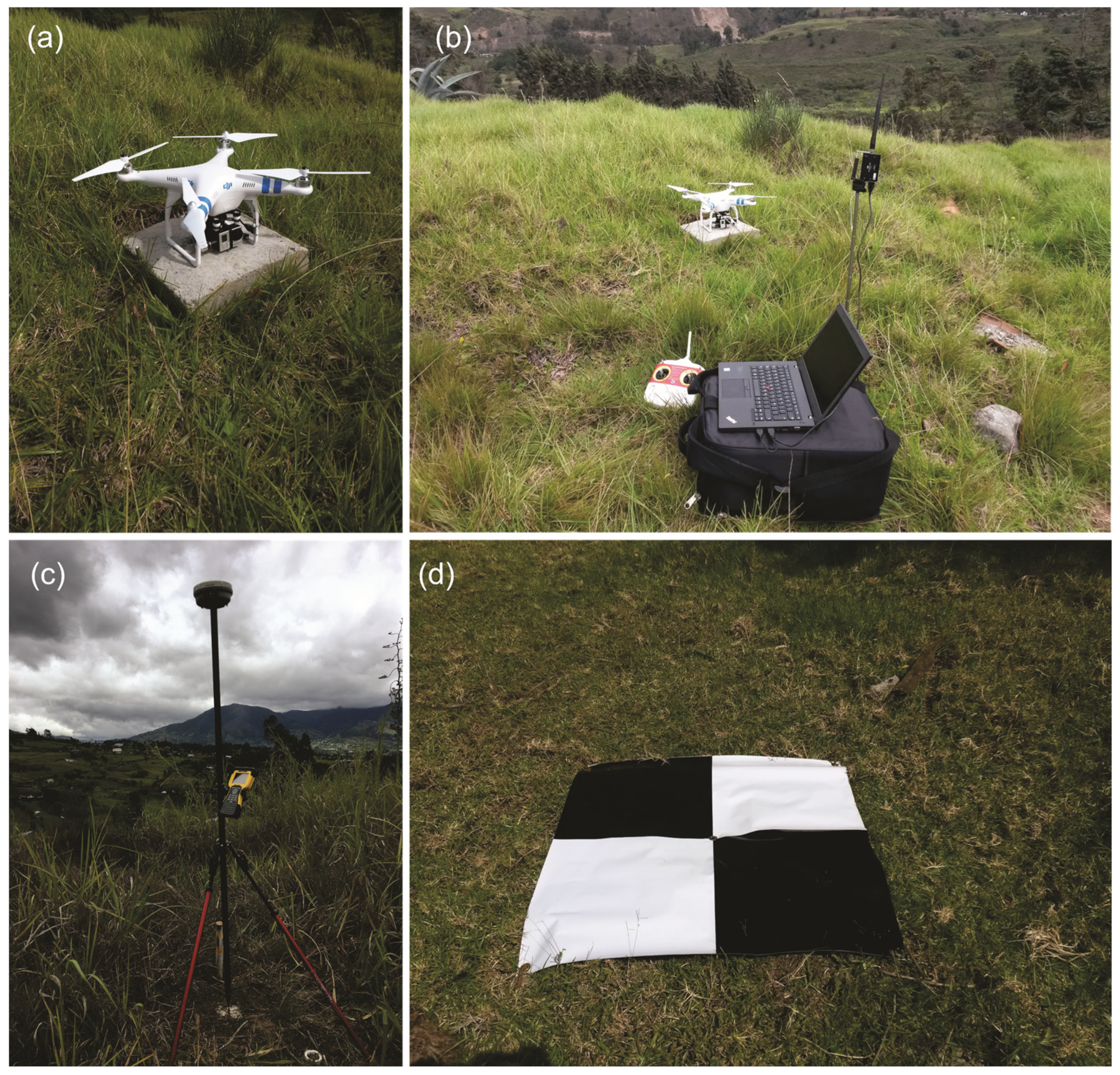
The RPAS used in this study consisted of a DJI Phantom 2 vehicle (Figure 3a) with the following specifications: a maximum horizontal range of 1000 m, maximum horizontal speed of 12 m/s, ascent speed of 6 m/s, descent speed of 2 m/s, net weight including the battery of 1 kg, horizontal displacement accuracy of 2.50 m, vertical displacement accuracy of 0.80 m, operating angle and temperature range from −10 to 50 °C. It was equipped with a Zenmuse H3-3D gimbal made of aluminum alloy, which maintained the camera’s position fixed in three axes using an Inertial Measurement Unit (IMU). The gimbal weighed 22 g (excluding the camera) and was compatible with GoPro and MAPIR cameras. The power for the gimbal was supplied by a DJI Phantom 2 intelligent battery.

For autonomous flight of the RPAS, the DJI 2.4 GHz Datalink system (Figure 3b) was used, enabling communication between the ground base and the aerial system through bidirectional data communication modules. This system allowed the flight plan to be loaded onto the RPAS via Bluetooth for subsequent execution. Flight planning and execution were carried out using the DJI Ground Station Version 1.4.63 application. Images were captured using a GoPro Silver Edition 3+ camera with a resolution of 10 Mp. The image capture interval was set to 2 s.

The ground control point (GCP) coordinates were measured using the differential GNSS technique with a Trimble R6 GNSS receiver (Figure 3c).

2.3. Methods

The methodology employed can be summarized as follows:

(1)

Data capture of images from Remotely Piloted Aircraft Systems (RPASs) and ground control points (GCPs) measurement using differential GNSS; software used Trimble Business Center (TBC) [58];

(2)

Processing of photogrammetric blocks and generation of DEMs and orthophotographs; software used: Agisoft Photoscan V 1.4.5 [29,35,59,60];

(3)

Generation of DoDs, profiles, and derivative models by a Geographic Information System (GIS); software used: QGIS V 3.30.0–ArcGIS 10.2.2 [61,62,63];

(4)

Mapping, morphometric analysis, and evolutionary assessment; software used: QGIS V 3.30.0, SAGA GIS V 9.0.1 [64];

(5)

Geotechnical characterization of materials.

2.3.1. Data Capture: Images and GCPs

The investigation of the slope movement in the El Plateado sector was conducted from 24 January 2017 to 12 March 2020, during which 4 RPAS campaigns were carried out for image capture.

Table 1. Details of RPAS missions in the study area.

RPAS Mission	Control 1	Control 2	Control 3	Control 4
Date	24 January 2017	9 June 2017	8 June 2018	12 March 2020
RPAS drone	Phantom 2
Camera	GoPro Silver Edition 3+
Flight height (m)	84.2	87	87.6	89
Area (km2)	0.265	0.285	0.258	0.251
Resolution (cm/pix)	4.20	4.33	4.10	4.00
Number of images	327	489	335	356
Longitudinal overlap (%)	70	70	70	70
Transversal overlap (%)	70	70	70	70
Number of GCP	9	9	9	9
X error (m)	0.022	0.033	0.036	0.028
Y error (m)	0.028	0.024	0.039	0.021
XY error (m)	0.036	0.041	0.053	0.035
Z error (m)	0.031	0.034	0.023	0.031
Number of CHK	6	6	7	6
X error (m)	0.011	0.023	0.036	0.014
Y error (m)	0.031	0.024	0.019	0.021
XY error (m)	0.033	0.033	0.041	0.025
Z error (m)	0.025	0.041	0.028	0.026

displays the dates and characteristics of the flights.

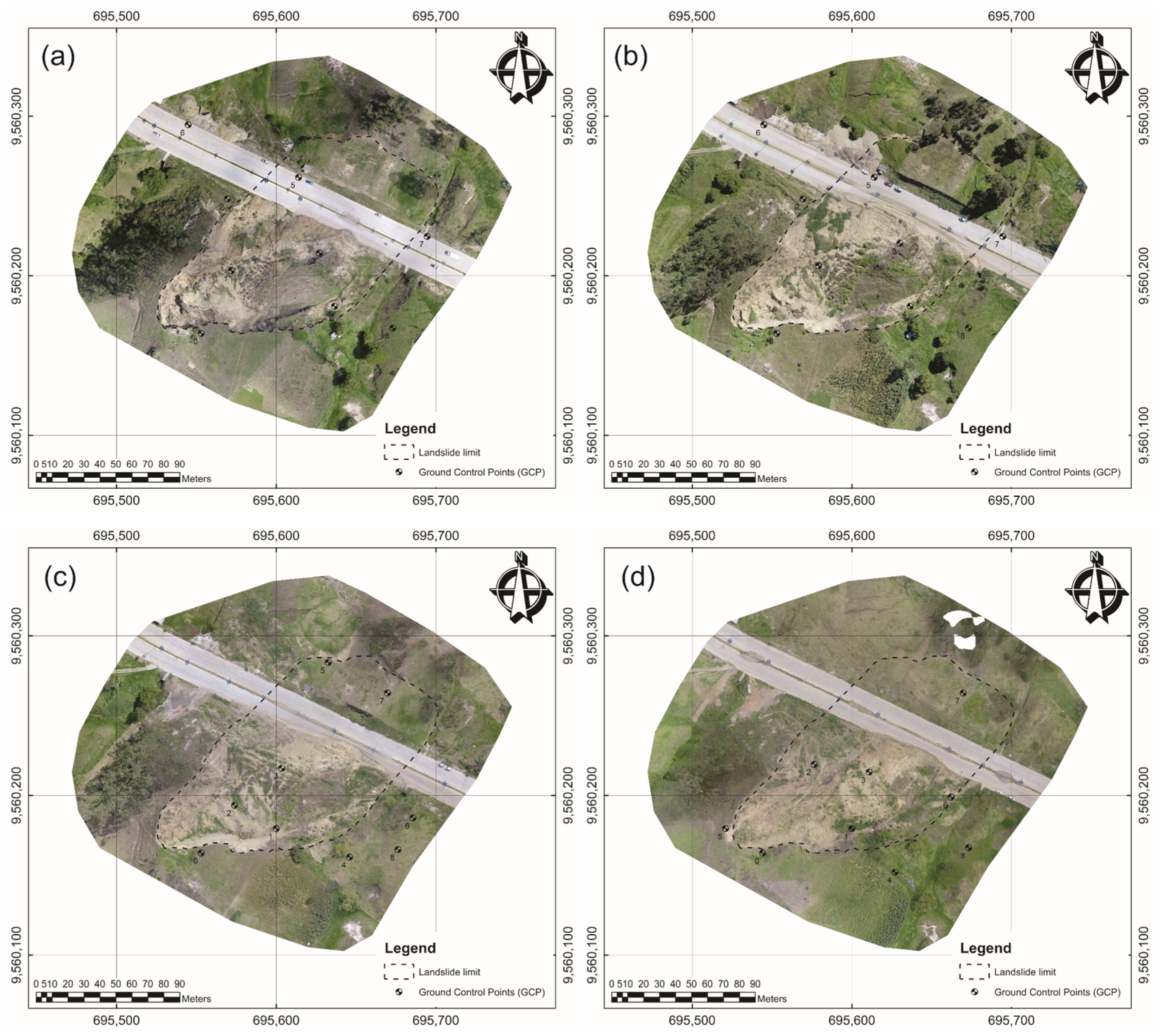
To provide photogrammetric support and orientation for the models, an in situ network of control and checkpoints was implemented. These points consisted of simple concrete markers with a diameter of 0.15 m and a depth of 0.30 m, with a steel rod of 12 mm diameter anchored at their center. Plastic markers measuring 1.00 m × 1.00 m were placed on the control points to ensure proper model orientation during the processing phase with the software (Figure 3d). Metal rings were installed at the center and ends of the markers, allowing for precise centering over the network points and fixation to the ground using metal hooks.

The coordinates of the control points were measured using differential GNSS technique employing a Trimble R6 GNSS receiver (Figure 3d) with an occupation time of 10 min at each point of the network. The post-processing of GNSS data used the data from the LJEC GNSS reference station of the Military Geographic Institute (IGM) belonging to the SIRGAS network and the Trimble Business Centre software version 2.6. The coordinates were oriented in the UTM WGS 84 zone 17 South coordinate system. The number of control and checkpoints is indicated in Table 1.

2.3.2. Photogrammetric Processing and Generation of Products

The aerial images obtained in the four RPAS campaigns were processed using Agisoft PhotoScan Professional software version 1.4.5. The accuracies achieved in the orientation process are shown in Table 1, and they are expressed as the root mean square error (RMSE).

The horizontal errors, both in the GCPs and the CHKs, ranged from 0.035 to 0.053 m, while the vertical errors ranged from 0.023 to 0.041 m, all of which were consistently below the recommended threshold of 0.10 m [40].

Subsequently, photogrammetric and SfM techniques were applied in the software to orient the photogrammetric blocks. Point clouds and dense point clouds were generated for the four processed flights, which were then filtered using a tool to remove outliers and noise. On average, the dense point clouds encompassed 11,238,000 points for the four flights. The result of this process was the corresponding digital elevation models (DEMs), which were exported in TIFF format for analysis in a GIS, with a resolution of 0.05 m.

Finally, orthophotos were also produced at a resolution of 0.05 m with the aforementioned accuracy being below the pixel size. The orthophotos can be used to delineate landslides in relation to the surrounding environment as well as to identify features such as scarps, cracks, etc., through photointerpretation.

2.3.3. Generation of DODs, Profiles and Derivative Models

First, the DEM of differences (DoD) is obtained using raster calculators in the GIS. For the surface monitoring of landslides, at least two data acquisition periods are required [65]. In the case of multitemporal analysis [25,27,57], the DEMs are compared in pairs. DoDs allow for the observation of vertical changes rather than vertical displacements. In fact, in many cases, what is observed are horizontal displacements and advances of the mass, which result in modifications of the DEMs [24,26,57]. DoDs can have negative values when the surface is lower in the later date and positive values when the surface is higher in the later date. Thus, excluding changes due to vegetation growth or decline, construction activities, and human interventions on the terrain (excavations, flattening, or fillings), natural changes in the surface of the terrain can occur due to surface descents (negative DoDs) in scarps and head areas, or horizontal displacements that result in excavation (negative DoDs) or accumulation of material (positive DoDs) in different areas of the landslide (head, body or foot).

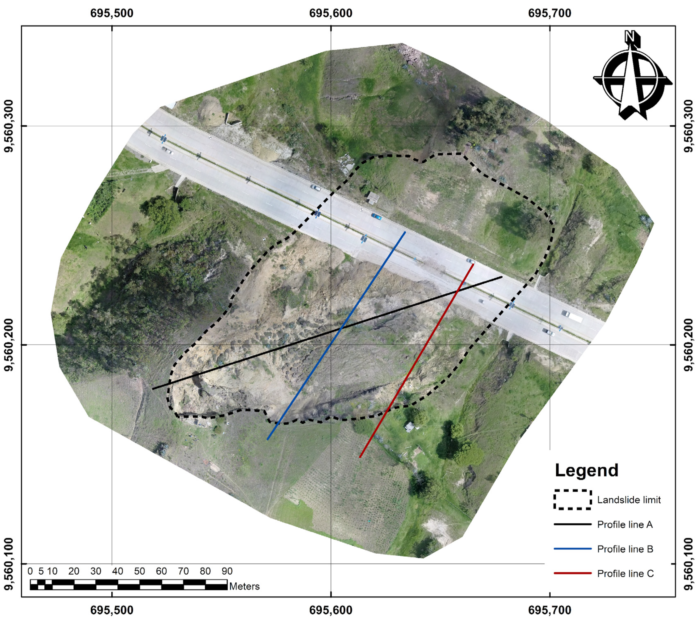
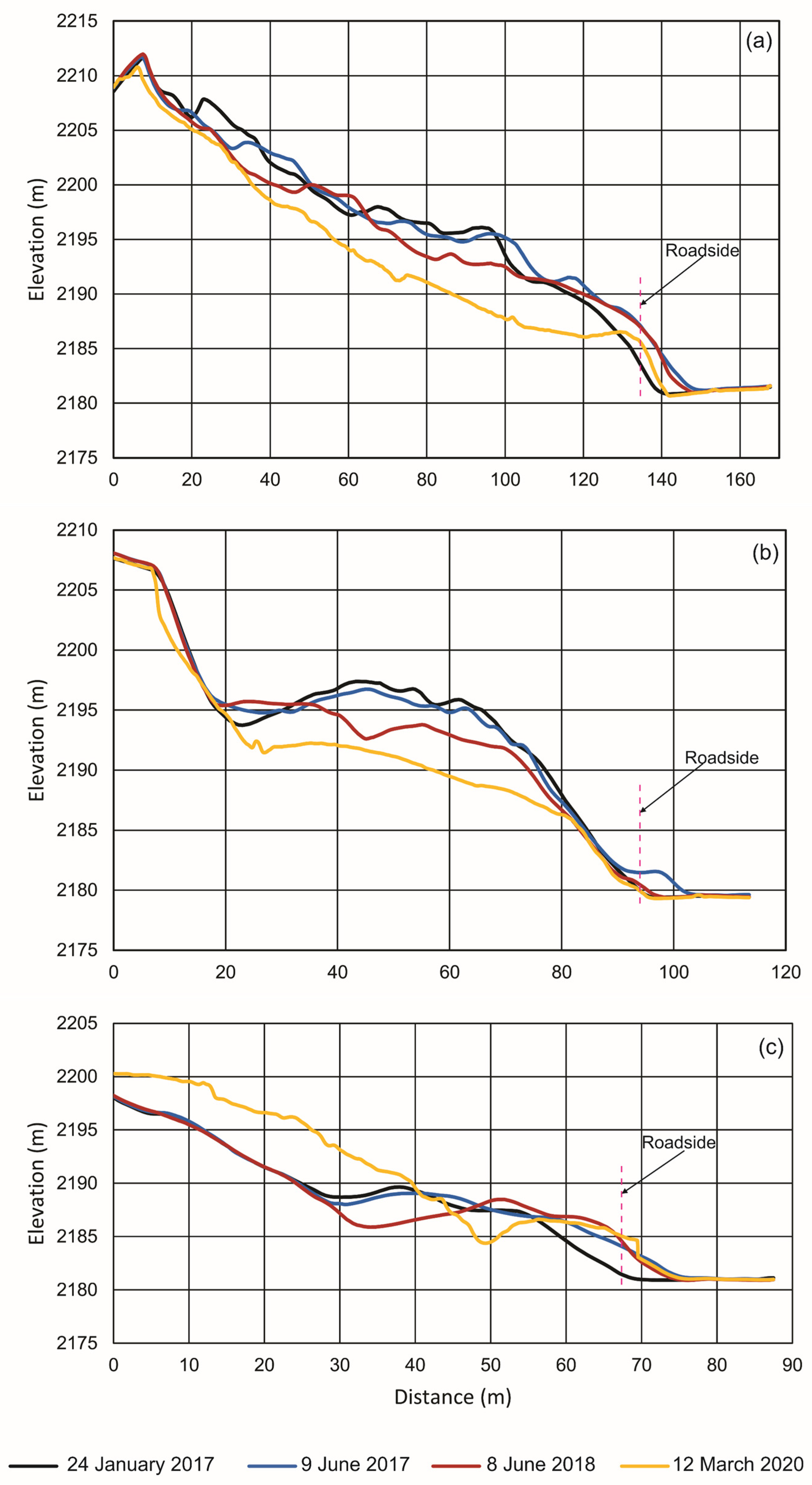
Second, to analyze the topographic parameters in the study area, profile lines were established, as shown in Figure 4. Profiles were generated based on the DEMs using Profiles tool in ArcGIS software, with a horizontal sampling interval of 0.50 m. The placement of the profiles considered soil displacements observed during field inspections and surface features. Profile A is longitudinal with a direction of N72°E, Profiles B and C are oblique with a direction of N33°E and N30°E, respectively, where B is more centered and C is more displaced to the foot area. The profiles provide a clear visualization of the topography and microtopography of the slope and the landslide, including all characteristic features such as scarps, head area, main body, foot, toes, and even cracks. By comparing the profiles, the changes in topography over time, the movement (downward and forward) of the mass, and its eventual retreat can be observed.

Lastly, in the third step, various derived models from the DEM have been obtained. These models consist of a series of topographic parameters that characterize the morphology of the slope and extract terrain features, focusing specifically on the main landslide but also on other instability processes observed in the study area. The derived models include slope angle, slope aspect, topographic position index (TPI), terrain roughness index (TRI), and topographic wetness index (TWI) for each analyzed date.

Slope angle or simply slope is the most relevant factor in determining slope stability [52,53,66,67,68,69,70]. Alterations in slope can increase shear stresses within the soil mass due to gravitational forces, leading to slope failure. Depending on the slope gradient, slow or rapid surface movements can occur.

Slope aspect or orientation, defined as the direction of the terrain’s inclination in each cell, influences the physical properties of soils primarily through the effects of rainfall, wind, and solar exposure [53,71,72,73].

The topographic position index (TPI) enables the description of morphological aspects of the terrain by determining and segmenting the hillslope [49,53,54,74,75,76]. It is calculated for the i-th pixel of the DEM elevation $h_i$, where $u_i$ represents the standard deviation of the DEM pixels and, ${\sigma }_i$ is the standard deviation of the DEM pixels within that same range. The calculation is given by Equation (1):

$$TPI=\frac{\left(h_i-u_i\right)}{{\sigma }_i}$$

(1)

The terrain roughness index (TRI) [50,54,77] is a measure that quantifies the variability of terrain height in a given area. It can be expressed using Equation (2):

$$TRI=\frac{{\sigma }_z}{Z_o}$$

(2)

where ${\sigma }_z$ is the standard deviation of the terrain heights and $Z_o$ is the mean height of the terrain surface. The result of the equation is a dimensionless number.

Finally, the topographic wetness index (TWI) [50,69,78] has been considered, which is related to the slope of a terrain and is used to identify areas where moisture or water accumulates. It is represented by Equation (3):

$$TWI=ln \left(\frac{a}{tan\beta }\right)$$

(3)

where a is the drained area for a specific cell, and tanβ is the slope of the analyzed cell.

For the determination of slope and aspect, ArcGIS V 10.2.2 software was used with the employment of Slope and Aspect tools, while QGIS V 3.30.0 and SAGA (System for Automated Geoscientific Analyses) V 9.0.1 software were used for TPI, TRI, and TWI [69].

2.3.4. Mapping, Morphometric Analysis, and Evolution Assessment

From DEMs and derivative models, terrain and hillslope forms in general and landslide features in particular can be identified and extracted. Slope and roughness (TRI) allow for the identification of scarps (steep slopes) and the body or foot of the landslide. However, it is the curvature or in this case the topographic position index (TPI) [51,52,53,54,79,80,81] that enables the identification of slope break lines and consequently delineates different parts of the movement. Specifically, the upper and lower break lines of scarps can be extracted. Additionally, other elements such as the foot of the landslides and especially its toe can also be detected [53].

The procedure involved obtaining the TPI map and symbolizing it with different classification and palette schemes to find the most appropriate thresholds for detecting break lines. The thresholds were ultimately set at +0.05 for the upper break line of scarps and −0.05 for the lower break line. Once the thresholds were selected, the skeletonization tool (SAGA tools) was applied to trace the lines (vectors) in shapefile format. The classified and color-symbolized rasters as well as the vectors from different dates can be used to observe the evolution of the scarps (for instance, retreat of main and lateral scarps and advancement of secondary scarps). Displacement measurements can be made using the measuring tool in GIS. Other resolutions different to the reference one at 0.05 m (e.g., 1 m) were also tested to better detect other features such as the toe, where the slope break is not as abrupt and thus more visible over a longer profile.

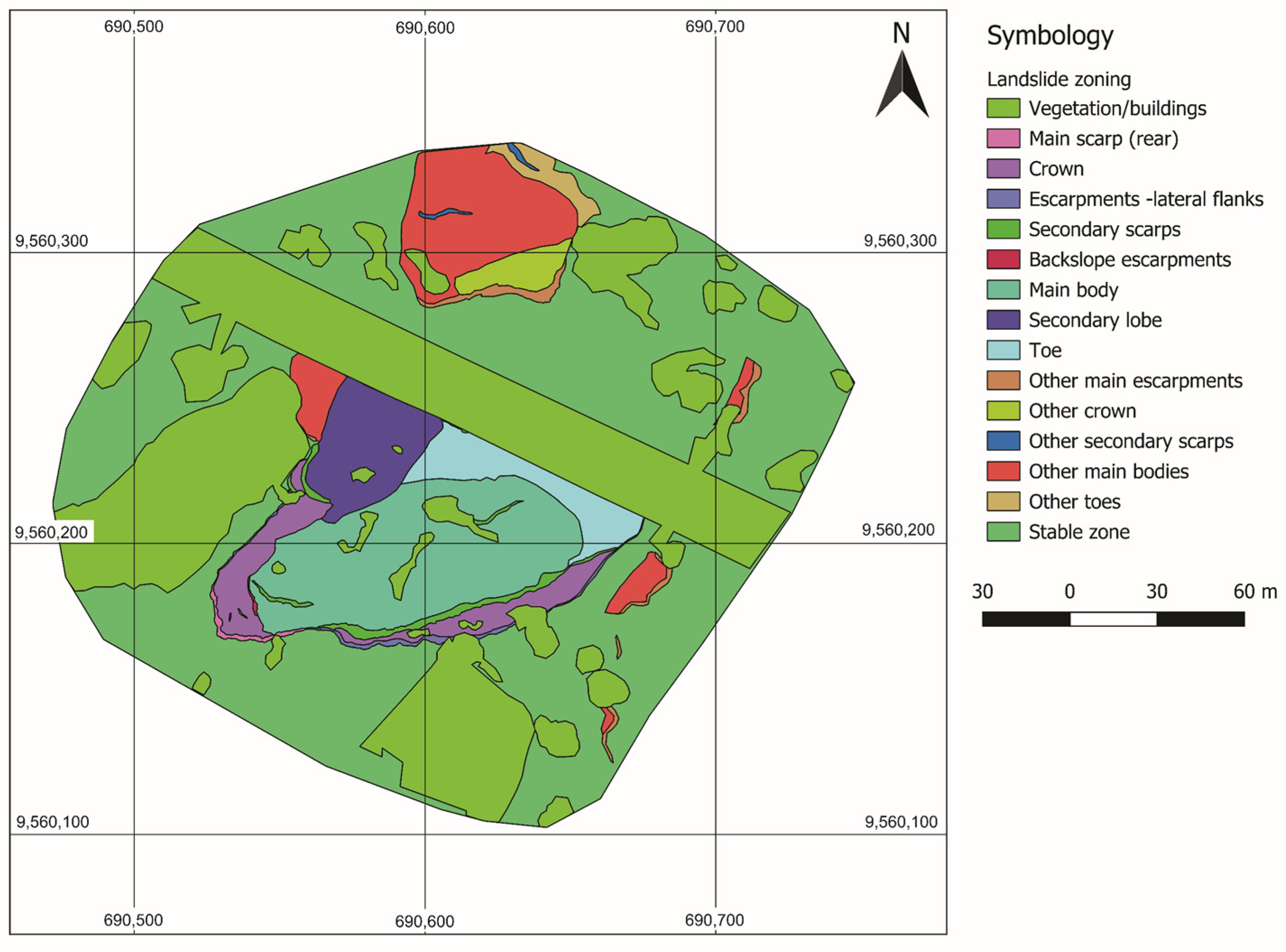
Finally, after identifying the main landslide elements and other features through photointerpretation, observation of the different derivative models, and the mentioned automatic extraction methods, a zoning of the study area was performed in order to analyze the characteristic morphometric parameters that define them. On one hand, landslide features and on the other hand, vegetation and constructions (roads, and buildings) were digitized. The latter were digitized to create masks that excluded the areas occupied by these elements from the analysis of characteristic landslide and terrain elements. In the case of vegetation, trees, shrubs, and undifferentiated areas of trees and shrubs were differentiated. Additionally, as support for photointerpretation, the alternative vegetation index GLI (Green Leaf Index) [82,83,84], which works with the native digital values of the red, green and blue (RGB) bands, was calculated.

Once the vector layers of landslide elements, unstable areas, vegetation, and constructions are obtained, they are rasterized. Subsequently, the raster calculator is applied to obtain a new raster excluding the vegetation and construction areas using Equation (4):

$$Raster=raster elements\times \left(raster vegetation-1\right)\times \left(raster constructions-1\right)$$

(4)

The elements identified and differentiated in the main landslide are as follows: main scarp, head, lateral flank and scarps, secondary and counterslope scarps, body, secondary body or lobe, and foot. Scarps, bodies, and foots of other minor instabilities in the study area were also detected.

Finally, the analysis of morphometric parameters (slope, aspect, TPI, TRI, and TWI) for the different elements was performed using zonal analysis tools (zonal statistics and zonal histogram) in QGIS.

2.3.5. Geotechnical Characterization of Materials

Laboratory tests were carried out on different soil samples (3 soil samples at the head, 3 samples at the body and 3 samples at the foot of the slope) all obtained at a depth of 3 m with an open pit. Using the Center-pivot backhoe loader 450, a Soil Moisture SM300 Kit was used to measure soil moisture (w%) at the time of extracting the samples for the respective analyses. The following tests were carried out in the laboratory, and the respective standards used for their execution are indicated:

• Water Content of Soil (ASTM D4643-17) [85];
• Liquid Limit, Plastic Limit, and Plasticity Index of Soils (ASTM D4318-17e1) [86];
• Particle-Size Analysis of Soils (ASTM D422-63) [87];
• Unified Soil Classification System (ASTM D2487-17e1) [88];
• Direct Shear Test of Soils Under Consolidated Drained Conditions (ASTM D3080) [89]

3. Results

3.1. Orthoimages and DEMs

The orthoimages obtained in the study area for the different flights are shown in Figure 5. Visual analysis of these orthoimages allowed for the identification of the main scarp, the head, the lateral flank and scarps, the secondary and counterslope scarps, the body, the foot, and other features. Among these, tension cracks in the head, body, and foot of the landslide were noteworthy both in longitudinal and transverse arrangement. At the crown level, the presence of induced cracks led to the failure of crown material, resulting in multiple scarps. The crown of the main scarp maintained a semicircular shape during the three observation periods. The landslide body could be clearly identified, as well as the accumulation zone at the foot and the advancement of material on one of the road lanes, as shown in Figure 5a–d. The main scarp was continuously eroded due to the material falling onto the slope body; however, its retreat was not very relevant, as will be discussed later.

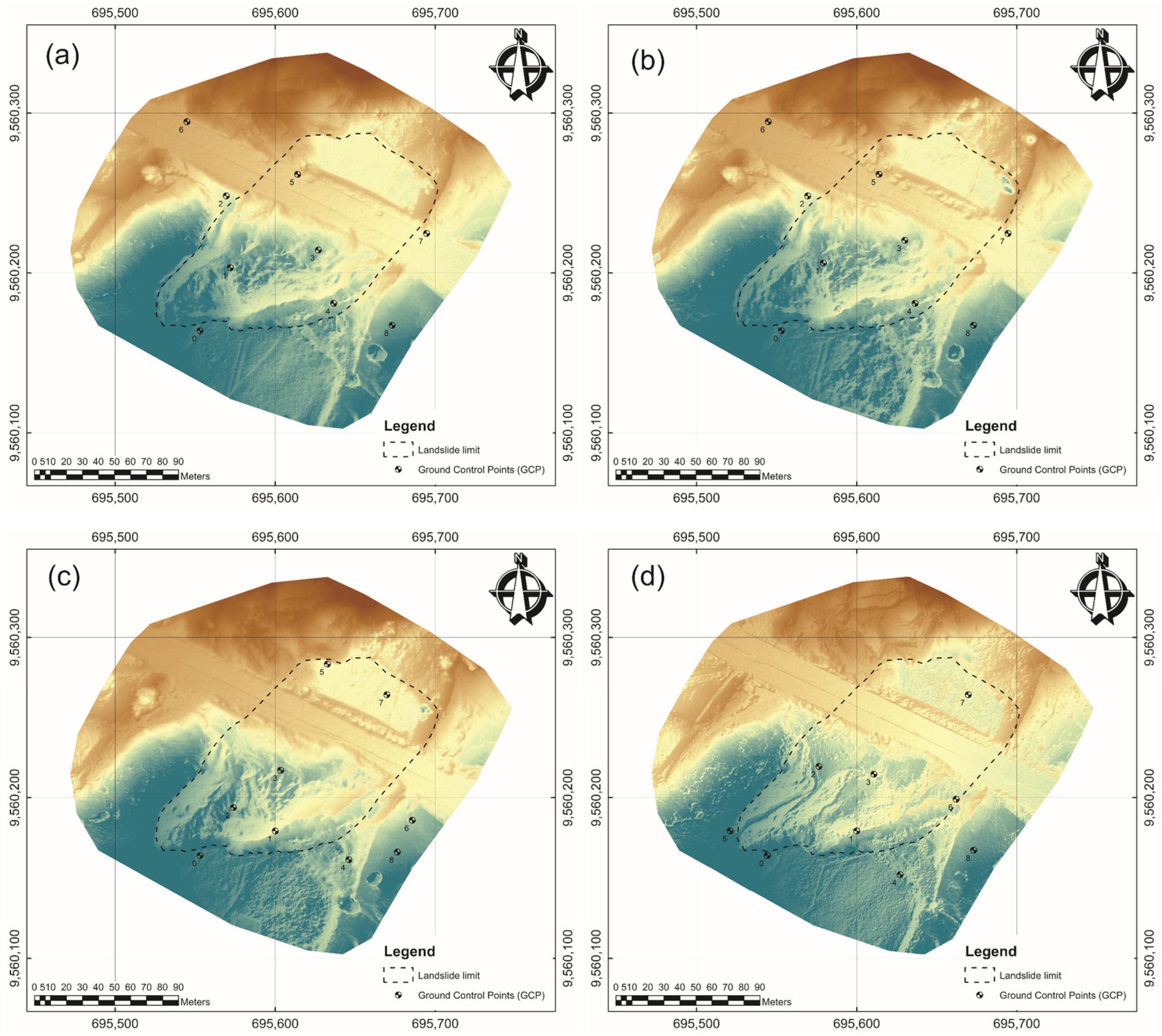
In Figure 6, the digital elevation models (DEMs) generated from the dense point cloud for the four-monitoring dates are displayed.

3.2. DEM of Differences (DoDs)

Figure 7 presents the DoDs of the El Plateado sector. The color palette was adjusted to visualize subtle movements in the DoDs. The color palette represents positive values (red) and negative values (green), with the former indicating an increase in terrain elevation and the latter indicating a decrease in terrain elevation.

The DoDs were generated from two study periods. The first period corresponds to January 2017 to June 2017; the second one covers from June 2017 to June 2018; and finally, the third one covers from June 2018 to March 2020. In the first period (Figure 7a), it is clearly visible that there are areas of terrain surface descent in the head and the upper part of the landslide body. Similarly, in the landslide body, there are areas of terrain surface descent related to secondary scarps and ascent due to the accumulation of material from the main scarp and secondary scarps. At the foot, the terrain surface ascent due to material accumulation or advancement is notable. As mentioned initially, points cloud filtering was performed to remove vegetation, although there were areas where filtering was not applied to preserve the topographic surface, as seen in the southern zone of the slope where positive values (light brown color) representing a surface elevation are observed, corresponding to vegetation growth (corn crops).

Figure 7b corresponds to the DoDs for the second period (June 2017 to June 2018). In both the head and the body of the landslide, areas of surface descent or ascent are identified, slightly displaced downhill compared to the previous period, indicating the progressive downslope movement of the slope, mainly in the ENE direction. In the foot, surface descent is observed, which is possibly related to the removal of material from the road. There is also clear evidence of instability under the road, with a material descent indicating the formation of a scarp.

In Figure 7c, a generalized descent is observed throughout the landslide body, which can be attributed to the anthropogenic action of material removal for slope stabilization carried out in early 2020.

3.3. Profiles

The results of the profiles (Figure 8) obtained from the DEMs allowed for the recognition of changes in the landslide body and foot corresponding mainly to horizontal displacements, taking the profiles obtained from the first DEM (24 January 2017) as reference. Profile line A, which corresponds to a longitudinal profile in the main direction of landslide progress from the crown at the WSW toward the foot at the ENE, clearly reveals different parts of the landslide: the main scarp and the head; followed by the body with a counterslope scarp in the upper part and secondary scarps in the lower part; and finally the foot that reaches the road. This same profile is observed in the subsequent dates (9 June 2017; and 8 June 2018), although it is displaced downslope and has less pronounced scarps due to the evolution of the landslide. These features allow for estimating greater mass descents and advances in the head and upper part of the body (total descent of about 6–8 m and advances of around 20–25 m; 3–4 m and 10–12 m in each period); while at the foot, the mass advances about 5–6 m, which may be underestimated due to material removal in the road area. However, the profile from the last date (12 March 2020) is different, showing a much more uniform slope from the crown area to the foot. Thus, what is observed is a flattening of the slope with material removal and the disappearance of the typical morphology, both in the scarp, in the body and even in the foot, where nevertheless a steeper slope is present in the road embankment.

In the case of profile line B, which represents an oblique profile from the right flank-scarp to the road, the main scarp is clearly observed in the first date, which is followed by the head with a slight counterslope toward the scarp. Further down the body, there is a convex shape, which then leads to a steeper slope toward the lower part of the body and the foot at the road. This shape remains consistent with time, although the surface gradually descends in the second and third dates. In the last date, there was smoothing of the slope shape from the scarp to the road, although a certain slope was still observable. We hardly observed any significant mass advancement in this profile due to its nearly transverse direction compared to the main movement direction.

Profile line C, parallel to the previous one but shifted toward the foot area, shows on the first date a more gentle right flank with almost no main scarp. Slightly below, the body exhibits a secondary scarp, and finally, there is a slightly steeper slope in the foot and road area. In the following two dates, there was a descent of about 3–5 m and a horizontal advancement of about 6–8 m, as expected in the foot area. However, this advancement could be attenuated by material removal from the road. In the last date, the change was minor and mainly corresponded to a surface descent due to slope repair works.

3.4. Topographic Parameter Maps

Before describing the topographic or morphometric parameters, the map of landslide elements and unstable zones (Figure 9) mentioned in Section 2.3.4 is presented. This map identifies the different types of scarps (main, lateral, secondary, counterslopes), the head, body, and foot of the main landslide, as well as other unstable zones present in the study area.

This zoning also serves for the analysis of the morphometric parameters presented in the following subsections.

3.4.1. Distribution and Evolution of Slope

Slope is the most important topographic parameter that describes the behavior of the terrain surface along time caused by slope kinematics [90]. Slope maps of the different monitoring dates are shown in Figure 10, and these allow for analyzing visually the temporal changes in slope distribution.

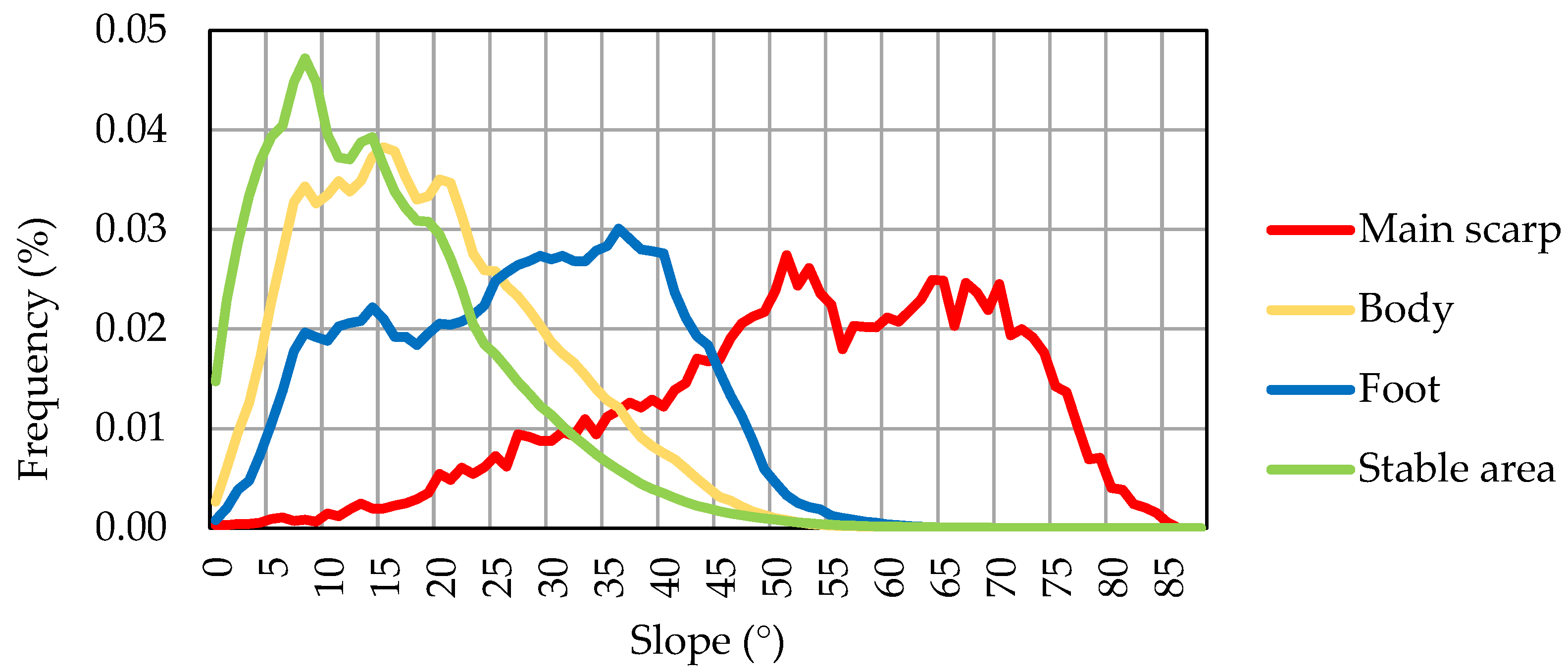
In the maps shown in Figure 10, areas with low slopes (<10°) can be observed on the road and the embankment below it as well as in the high and stable zone above the landslide crown. Areas with steep slopes (above 30°) can be seen in vegetated areas, especially trees and bushes, which need to be disregarded. Focusing on the landslide area, steep slopes are clearly observed in the different scarps (main, lateral, and secondary), while the slopes in the body are lower, alternating between flat areas with steeper slopes corresponding to secondary scarps. Slightly higher slopes are also observed in the foot area.

The slopes for the landslide elements for the first date are presented in

Table 2. Slope statistics for landslide elements.

Element	Average	Mode	Min.	Max.	Range	Std-D.	C.Var.
Main landslide
Main scarp	53.53	20.61	0.15	85.63	85.48	16.14	0.30
Head	23.25	20.48	0.00	75.60	75.60	12.39	0.53
Lateral scarps-flanks	40.97	19.12	0.56	83.23	82.67	16.08	0.39
Secondary scarps	43.65	25.46	0.30	82.28	81.98	13.67	0.31
Counterslope scarps	48.02	12.93	2.80	74.53	71.73	15.09	0.31
Body	19.84	7.10	0.00	77.69	77.69	10.60	0.53
Secondary body	26.75	25.46	0.07	81.11	81.04	12.49	0.47
Foot	27.76	25.46	0.07	70.36	70.29	12.50	0.45
Other landslides
Main scarps	40.95	32.01	0.00	83.05	83.05	13.60	0.33
Heads	18.83	12.93	0.00	74.74	74.74	10.41	0.55
Secondary scarps	35.99	14.64	1.05	65.63	64.59	13.54	0.38
Bodies	20.21	12.93	0.00	75.27	75.27	11.97	0.59
Foots	29.98	30.99	0.25	63.58	63.33	9.34	0.31
Stable area
Stable area	15.61	7.10	0.00	84.30	84.30	10.28	0.66

. It can be observed that the scarp areas have average slopes greater than 40° with the main scarp reaching nearly 54°. The head has a slope of 23.25°, the main body has a slope of 19.84°, and the foot has a slope of 27.76°. The overall slope of the landslide was 24.15° compared to the stable zone with a slope of 15.61°. Other unstable zones have average slopes of 22.59°, with the slopes of their scarps slightly lower than those of the main landslide scarps.

In Figure 11, the distribution of slopes in some of the different landslide elements is shown.

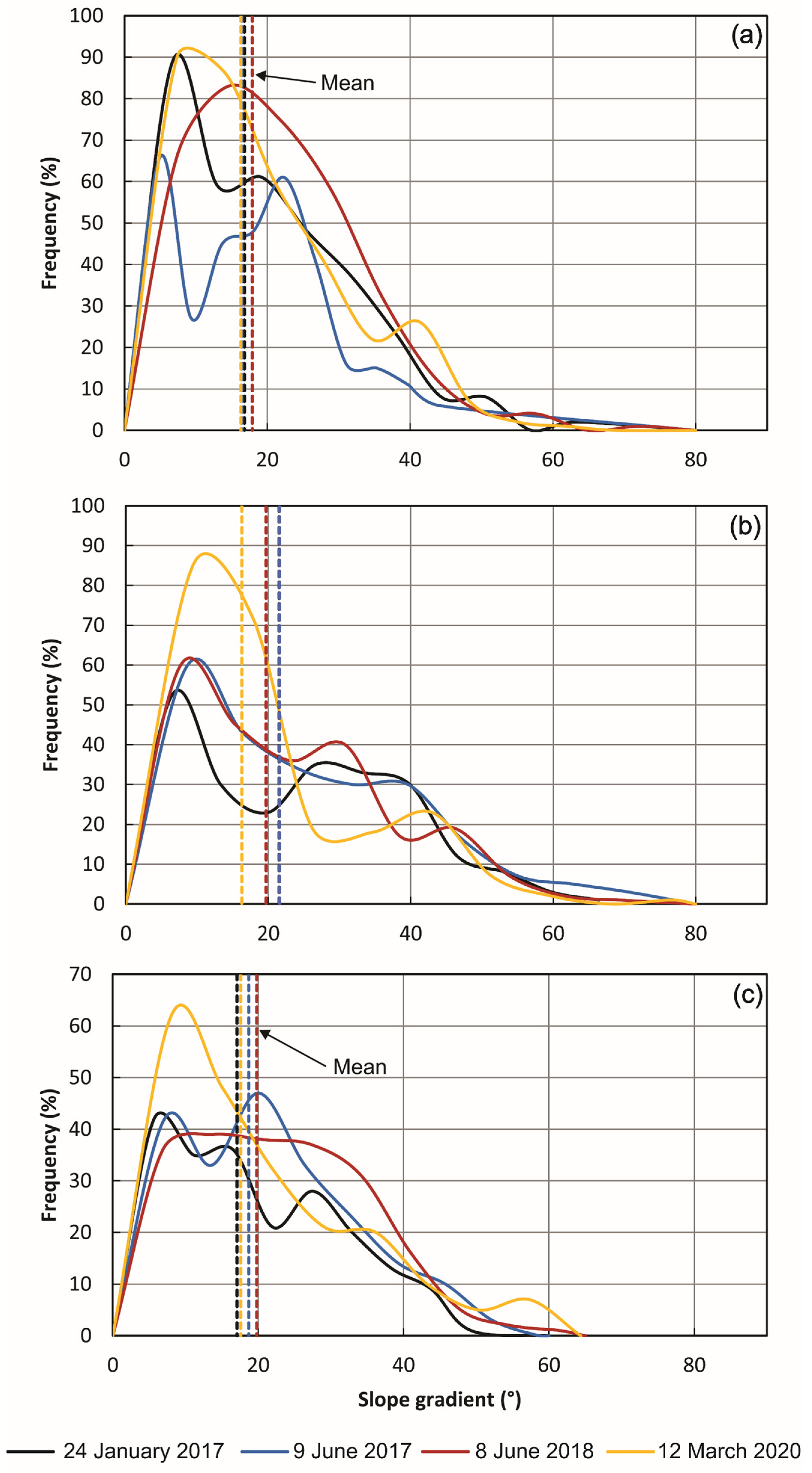
The evolution of the slope can be observed through their frequency distribution in each profile (Figure 12). In longitudinal profile A, taking the first date (24 January 2017) as a reference with an average slope of 18.11°, a gradual decrease in slope is observed, becoming 17.75° in the second date, 16.72° in the third date, and more significantly in the fourth date, decreasing to 13.30°. In profile B, oblique to the direction of the landslide and with an initial average slope of 21.79°, the trend is a progressive decrease, reaching 21.40° in the second date, 20.40° in the third date, and 18.10° in the fourth date. Meanwhile, profile C, which is located more marginally than the others, starts with an initial average slope of 17.43° but exhibits different and more irregular behavior. In the second date, it increases to 20.24°, after which it decreases to 18.70° in the third date and increases again to 21.42° in the fourth date.

The frequency of slopes below 20° increases in each profile. In profile A, it starts at 60%, slightly decreases in the second date to 58%, then increases significantly in the third date (65%) and particularly in the fourth date (76%). In profile B, a similar pattern is observed with an initial percentage of 46%, which slightly increases in the second date and further increases in the third (52%) and fourth (64%) dates. Profile C starts at 66%, decreases in the second date to 56%, increases in the third date to 68%, and decreases again in the fourth date to 60%.

3.4.2. Distribution and Evolution of Aspect

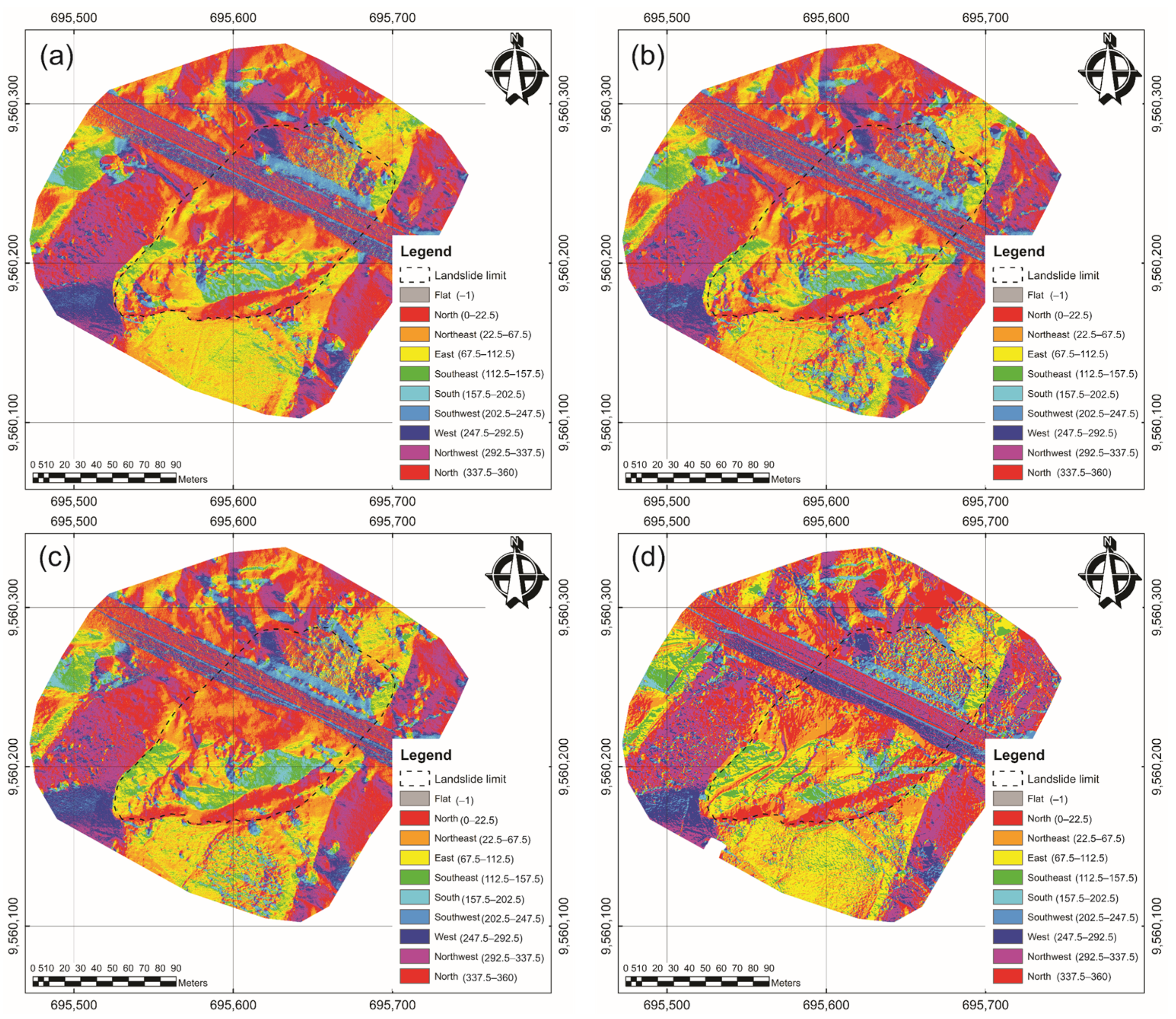
Figure 13 displays the aspect maps of the study area for the four monitoring dates.

In the maps shown in Figure 13, a set of slope units alternately oriented toward the NW and SE can be observed, the landslide slope being oriented toward the NE but with a wide range between the N and SE directions. There are also some localized areas in the landslide with slopes facing the SW. This general arrangement remains consistent in all analyzed dates, although the counterslope areas (between the S and W) generally appear downslope in the other dates, except for the last date where they practically disappear.

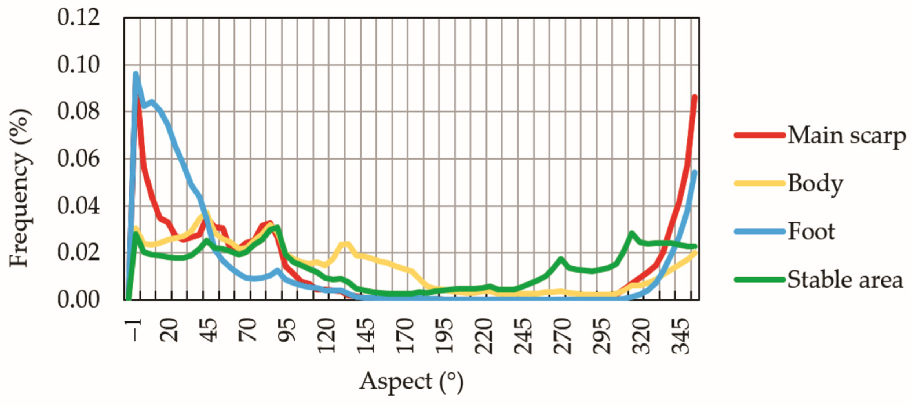
In the element analysis for the first date presented in

Table 3. Aspect statistics for landslide elements.

Element	Average	Mode	Min	Max	Range	Std-D.	C.Var.
Main landslide
Main scarp	68	0	0.00	359.99	359.99	139.43	1.05
Head	90	90	0.00	359.98	360.98	104.06	0.91
Lateral scarps-flanks	89	0	0.00	359.99	359.99	130.09	1.02
Secondary scarps	64	0	0.00	359.98	359.98	154.46	0.94
Counterslope scarps	271	270	1.28	358.73	357.45	29.81	0.11
Body	91	90	0.00	359.97	360.97	99.17	0.82
Secondary body	46	0	0.00	359.98	359.98	124.71	1.18
Foot	31	0	0.00	359.97	359.97	120.77	1.40
Other landslides
Scarps	313	0	0.00	359.99	360.99	107.93	0.40
Heads	280	0	0.00	359.97	360.97	121.74	0.52
Secondary scarps	110	180	0.00	358.79	358.79	74.40	0.68
Bodies	267	0	0.00	359.98	360.98	142.33	0.76
Foots	32	0	0.00	359.97	359.97	101.22	1.56
Stable area
Stable area	124	0	0.00	359.98	359.98	123.87	0.72

and Figure 14, it can be observed that the main scarp has an average orientation toward the NE although with several relative maxima toward the N and E. The secondary scarps have a similar average orientation to the NE, while the lateral scarps face the E, with two maxima toward the SE and N, corresponding to the left and right flanks, respectively. Finally, the counterslope scarps are oriented toward W. The body has an orientation in a wide range between the N in the lower part and the S in the upper part. The orientation of the foot is highly concentrated toward the NNE. The other unstable areas exhibit variable orientations, while the stable zone shows a relatively insignificant average with maxima between the N and E or even the NW.

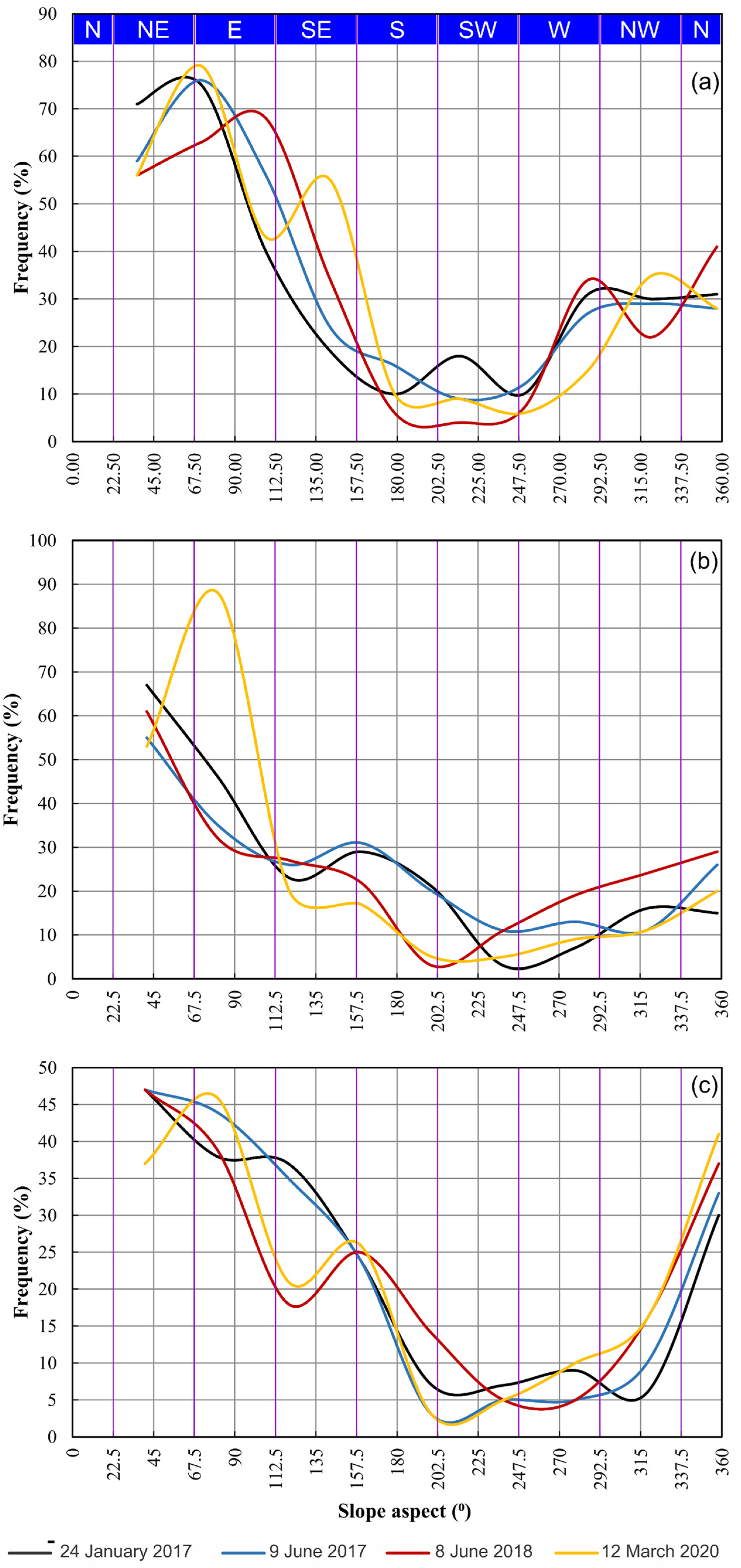
The evolution of orientation in profile A (Figure 15a) starts in the first date with a predominant orientation toward the N and NE (scarp, body and foot), although there is also a relative maximum toward the south (upper part of the body and counterslope scarps). From there, the majority orientation gradually shifts more toward the NE, reducing the orientations toward the S and W.

In profile B (Figure 15b), a similar pattern is observed, with an absolute maximum orientation toward the N and NE in the first date, along with a relative maximum toward the south. In the following two dates, no significant changes are observed although the orientations toward the south decrease. In the last date, this trend continued, but the absolute maximum clearly shifted toward the east–northeast.

Finally, in profile C (Figure 15c), the orientation is distributed between N and E in the first date, remaining similar in the second date. In the third date, a relative maximum appears toward the SE, and in the fourth date, the maximum shifts toward the NE.

3.4.3. Distribution and Evolution of the Topographic Position Index (TPI)

Figure 16 displays the maps of the topographic position index (TPI) at a 1 m resolution for the four considered dates.

In these maps, there is a general predominance of TPI values close to zero throughout the area, with concentrated sectors that are elongated in a certain direction, alternating between positive and negative values. These sectors correspond to areas with clear slope breaks, which correspond to the upper and lower boundaries of the main scarp as well as the lateral and secondary scarps.

In the element analysis of the TPI at 0.05 m resolution for the first date, as shown in

Table 4. TPI statistics for the landslide elements.

Element	Average	Mode	Minimum	Maximum	Range	Std-D.	C.Var.
Main landslide
Main scarp	0.00	−0.02	−1.04	0.88	1.92	0.13	−103.11
Head	0.00	0.00	−0.35	0.36	0.70	0.02	−11.94
Lateral scarps-flanks	0.01	0.00	−0.63	0.40	1.03	0.06	9.27
Secondary scarps	0.00	0.00	−0.52	0.56	1.09	0.05	40.75
Counterslope scarps	0.00	−0.03	−0.26	0.31	0.57	0.08	−55.03
Body	0.00	0.00	−0.28	0.35	0.63	0.02	−28.22
Secondary body	0.00	0.00	−0.40	0.39	0.79	0.02	−23.97
Foot	0.00	0.00	−0.19	0.21	0.40	0.02	−217.18
Other landslides
Scarps	0.00	0.00	−0.54	0.81	1.35	0.05	−188.40
Heads	0.00	0.00	−0.17	0.43	0.60	0.02	−8.23
Secondary scarps	0.00	0.00	−0.22	0.17	0.39	0.04	58.95
Bodies	0.00	0.00	−0.25	0.24	0.49	0.02	−17.44
Foots	0.00	0.00	−0.20	0.20	0.39	0.02	−12.25
Stable area
Stable area	0.00	0.00	−0.68	0.53	1.21	0.01	108.33

and Figure 17, all elements and zones show average values close to zero. The differences occur in the range and, especially, the standard deviation, which is higher in the scarps, particularly in the main scarp (0.13), and lower in the body and foot of the landslide (0.02) as well as in the stable zone (0.01), which shows the least variability among all the analyzed zones.

Meanwhile, Figure 18 displays the results of applying the skeletonization tool on the four-measurement dates for TPI at 1 m resolution, showing the corresponding extracted lines. The lines representing the upper boundary (blue) and lower boundary (red) of the scarps are clearly visible.

Throughout the different analyzed dates, excluding areas with vegetation changes, changes in the position of the upper and lower slope break or edge lines of the scarps can be observed, particularly the upper lines of the main scarp and the lateral scarps, which show a retreat toward the upper part of the slope, as will be discussed later. Meanwhile, the lower lines of these scarps exhibit less variation, and the lines of other scarps are more discontinuous and irregularly distributed throughout the landslide area. Regarding the foot area, the line defined by the tip is identified by the lower break or edge line of the TPI at 1 m resolution. In this case, advancements of the lines in the downslope direction can be observed, occupying the road area in the second and third dates, with a retreat in the fourth date.

3.4.4. Distribution and Evolution of the Terrain Roughness Index (TRI)

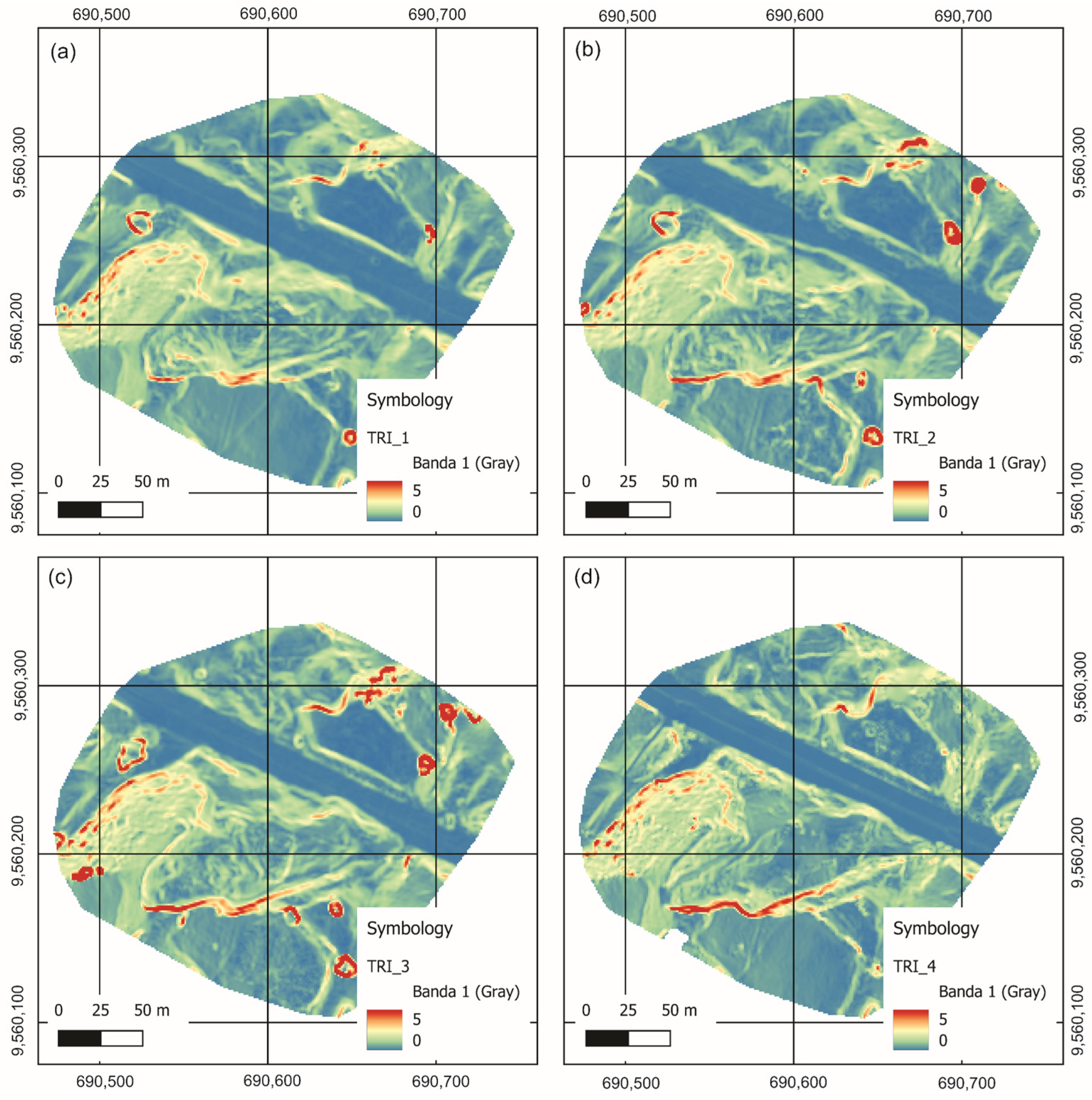
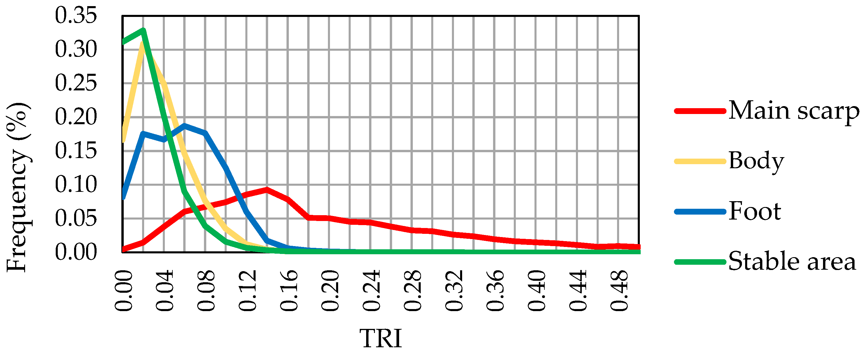
In the maps of Figure 19, areas of high roughness can be observed, particularly in relation to the scarps, especially the main scarp and the lateral scarps, but also in the secondary scarps and the foot of the main landslide, while the landslide body exhibits low roughness. Areas of relatively high roughness are also observed in the scarps of other minor landslides, while the stable zone presents the lowest roughness if areas with vegetation are excluded.

The roughness values for the different landslide elements are shown in

Table 5. TRI statistics for the landslide elements.

	Average	Mode	Min.	Max.	Range	Std-D.	C.Var.
Main landslide
Main scarp	0.22	0.05	0.00	1.60	1.59	0.16	0.71
Head	0.06	0.05	0.00	0.52	0.52	0.04	0.65
Lateral scarps-flanks	0.13	0.04	0.00	1.03	1.03	0.09	0.68
Secondary scarps	0.13	0.06	0.00	0.90	0.90	0.07	0.55
Counterslope scarps	0.16	0.03	0.01	0.44	0.43	0.09	0.52
Body	0.05	0.02	0.00	0.56	0.56	0.03	0.61
Secondary body	0.07	0.03	0.00	0.78	0.78	0.04	0.58
Foot	0.07	0.06	0.00	0.34	0.34	0.04	0.53
Other landslides
Scarps	0.12	0.08	0.00	1.00	1.00	0.08	0.65
Heads	0.04	0.03	0.00	0.45	0.45	0.03	0.64
Secondary scarps	0.10	0.03	0.00	0.27	0.27	0.05	0.50
Bodies	0.05	0.03	0.00	0.47	0.47	0.03	0.69
Foots	0.07	0.07	0.00	0.24	0.24	0.03	0.37
Stable area
Stable area	0.04	0.02	0.00	1.22	1.22	0.03	0.76

and Figure 20. It can be observed that the scarps have an average roughness of 0.14, which is slightly higher in the main scarp (0.22). Meanwhile, the head area shows an average roughness value of 0.06, which is slightly higher than the body (0.05) and lower than the foot (0.07). The other instability areas exhibit generally lower but comparable values, which are always higher than the stable zone (0.04).

The evolution of roughness observed in the maps is relatively smooth at the overall landslide level and is mainly concentrated in the scarps, where roughness increases in the second and third dates. Changes in the position of high-roughness areas can be observed in the body and foot areas due to landslide displacement. However, in the fourth date, a general decrease in roughness can be observed in the body and foot. Some changes can also be seen in other unstable zones, especially the one occurring under the road, over the entire analyzed period.

3.4.5. Distribution and Evolution of the Topographic Wetness Index (TWI)

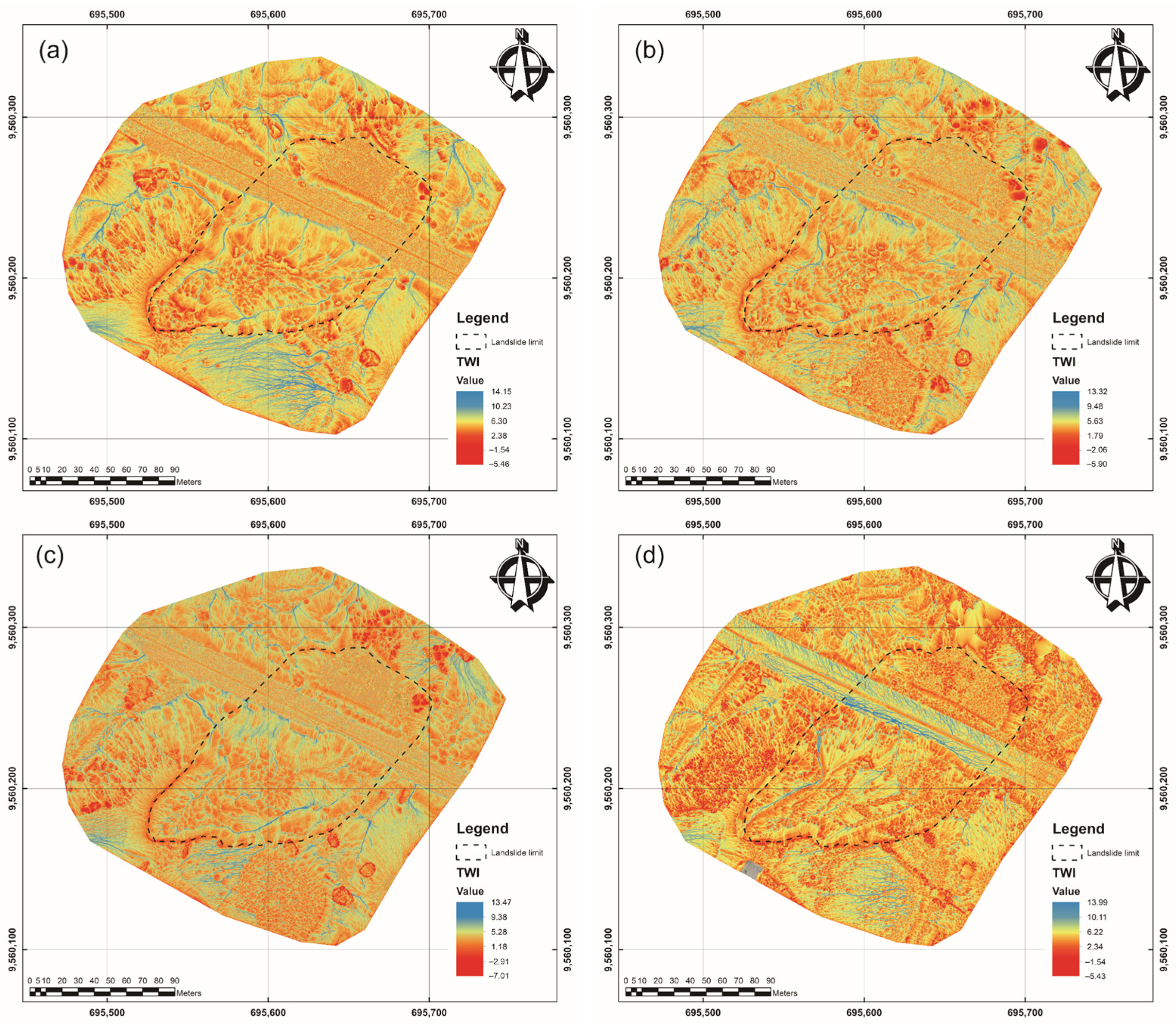
Figure 21 shows the distribution of TWI for each monitoring date, where higher positive TWI values are represented in shades of blue. These areas indicate a high potential for water accumulation or surface water runoff, primarily from rainfall, thus representing in some way the drainage network of the slope. Negative values correspond to areas where water accumulation is not possible, generally corresponding to the higher parts of the slope.

Thus, it can be observed that in the upper part of the landslide, near the main scarp and lateral scarps, the values are low, gradually increasing in the head and along the body where a drainage network formed within the landslide. Two drainage lines stand out on both sides of the body, between it and the scarps, which developed from the cracks generated by friction and displacement of the mass. Additionally, it is important to note how the different networks converge in the foot zone and the road, where the highest index values are reached. The remaining sectors of the study area outside the movement show a better organized drainage network except in the areas of crops and vegetation, which are more irregular. The drainage configuration changed throughout the analyzed dates, with a tendency to accumulate higher index values in the foot zone around the road from the first to the third date, while in the last date, the area shows a less hierarchical and more irregular drainage structure.

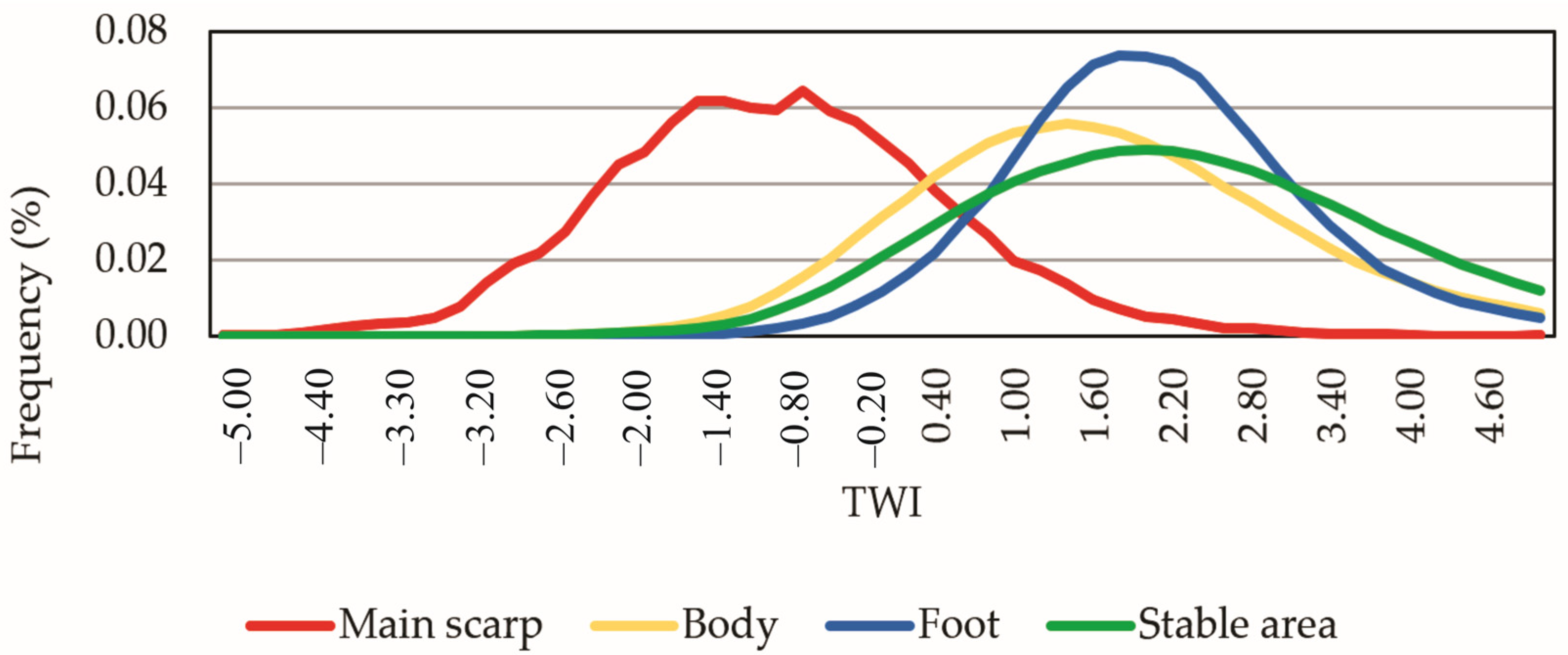
These observations are corroborated by the results of the element analysis shown in

Table 6. TWI statistics for the landslide elements.

	Average	Mode	Min.	Max.	Range	Std-D.	C.Var.
Main landslide
Main scarp	−0.69	−2.65	−5.25	7.95	13.19	1.28	−1.85
Head	1.74	2.83	−4.55	12.18	16.72	1.51	0.87
Lateral scarps-flanks	1.02	−1.03	−4.73	8.43	13.16	1.55	1.52
Secondary scarps	1.04	−2.76	−5.34	7.11	12.44	1.39	1.33
Counterslope scarps	−0.24	−4.15	−4.15	5.11	9.26	1.44	−6.00
Body	1.88	2.83	−4.46	13.57	18.03	1.59	0.85
Secondary body	2.06	0.59	−4.98	13.74	18.72	1.53	0.74
Foot	2.22	2.83	−3.56	11.50	15.05	1.21	0.54
Other landslides
Scarps	1.35	−1.34	−5.24	7.31	12.55	1.32	0.98
Heads	2.01	0.75	−4.72	11.71	16.44	1.39	0.70
Secondary scarps	0.77	2.68	−3.40	6.78	10.18	1.04	1.35
Bodies	2.35	2.83	−4.17	14.15	18.32	1.56	0.67
Foots	2.07	0.62	−3.86	8.54	12.41	1.23	0.59
Stable area
Stable area	2.38	2.83	−5.02	15.26	20.28	1.66	0.70

and Figure 22. Thus, the scarps have low values of the TPI index, especially the main scarp, which even presents negative values (−0.69). The remaining parts of the landslide show increasing values from the head (1.74), body (1.88), and foot, where the highest values are reached (2.22). The other unstable zones also show increasing values from the scarps (1.35) to the foot (2.07). Moreover, the stable zone presents even higher average values (2.38).

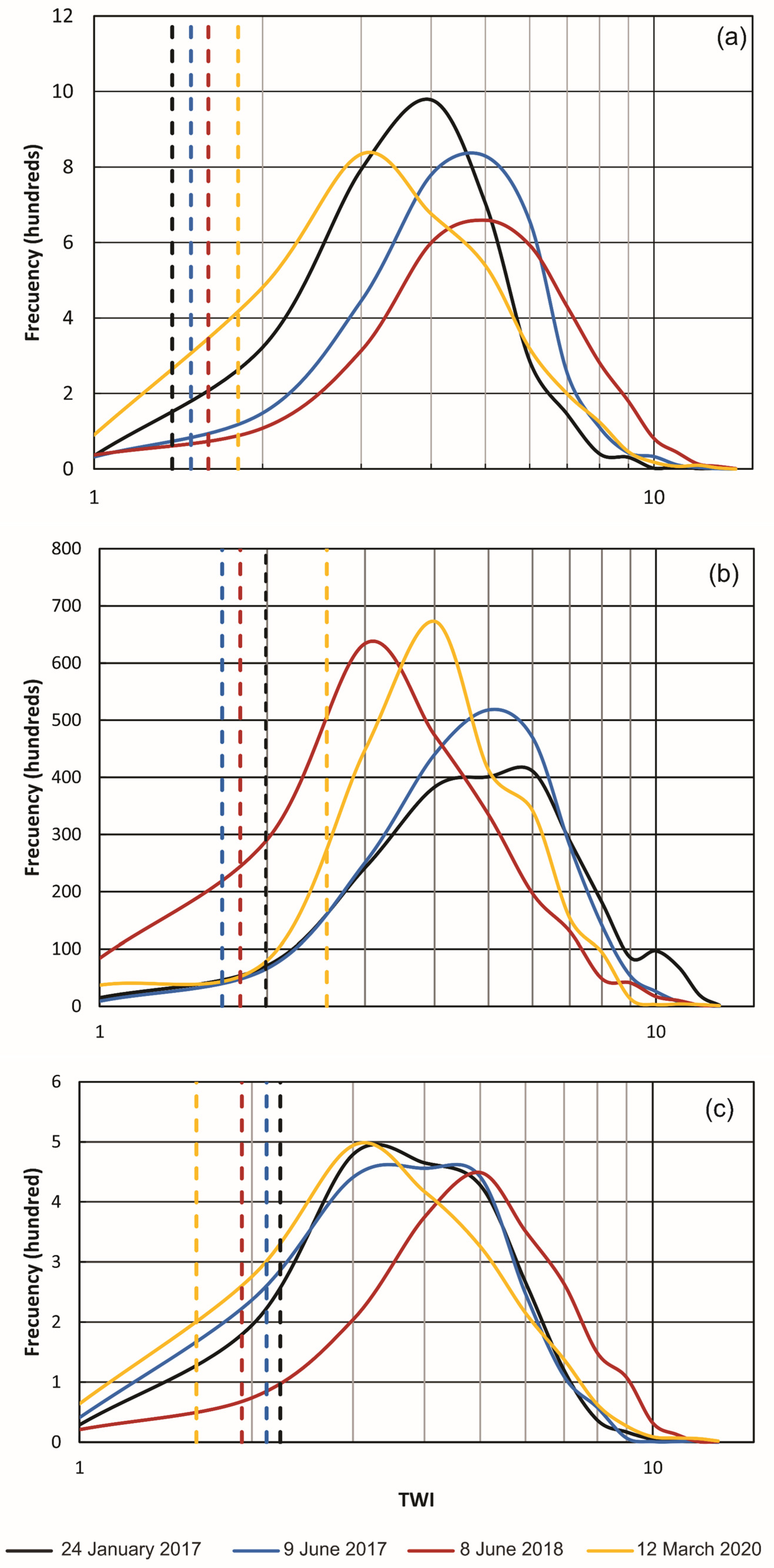
In Figure 23, the temporal changes of TWI in each profile are shown. In the case of longitudinal profile A (Figure 23a), it can be observed that the mean TWI values gradually increase from 1.38 (24 January 2017) to 1.49 (9 June 2017), 1.60 (8 June 2018), and 1.81 (12 March 2022), mainly in the foot area, as previously pointed out. In profile B (Figure 23b), which is oblique to the landslide, the mean TWI values are 1.99, 1.66, 1.79, and 2.56 for the considered date, showing an increasing trend of TWI in general. In profile C (Figure 23c), which occupies a more marginal position toward the foot area, a decrease in mean TWI values can be observed, from 2.24 to 2.12, 1.92, and finally to 1.60. The discussion will further analyze the variations of TWI and its relationship with the behavior of the slope movement.

3.5. Geotechnical Characterization of the Affected Materials

Table 7. Summary of laboratory test results conducted on soil samples obtained from the slope.

Ubication	Sampling	w (%) +	LL	w (%) *	LP	SUCS	ϕ	C (kg/cm2)
Crown	1	28.55	59.7	27.6	5.86	CH	27°	1.65
	2	28.00	59.4	27.3	6.04	CH
	3	28.26	60.1	27.4	6.17	CH
Body	1	34.22	67.9	33.8	38.3	MH-OH	22°	0.37
	2	34.12	67.0	33.8	37.6	MH-OH
	3	34.31	66.3	33.6	37.4	MH-OH
Foot	1	40.51	86.2	39.9	37.6	MH-OH	11°	0.34
	2	41.02	84.6	39.9	37.1	MH-OH
	3	40.74	86.0	39.1	38.7	MH-OH

⁺ Laboratory determined moisture content. * Moisture content measured in the field with Soil Moisture SM300 Kit.

shows the results of the tests conducted on soil samples. At the head, soils with high plasticity clay (CH) have been determined, while at the body and foot levels, inorganic silts (MH-OH) are present. LL represents the liquid limit, LP represents the plastic limit, SUCS is the system classification of soil, ϕ represents the friction angle, and C represents cohesion.

4. Discussion

4.1. Accuracy and Uncertainty of DEMs and Orthoimages

Considering the root mean square errors (RMSE) at the checkpoint (CHK) locations shown in Table 1, it can be observed that the horizontal errors (XY) range from 0.025 to 0.041 m through the different flights, which is even lower than those found in GCPs (0.035–0.053), and they are always below the 0.05 m resolution of the orthoimages and DEMs. Both these values and those calculated for the control points are similar to the errors obtained by other authors in RPAS surveys under comparable conditions [25,26,30,34,38,57,91,92]. Therefore, the uncertainty for horizontal measurements is established at 0.05 m.

Regarding vertical RMSE (Z), the obtained values vary from 0.025 to 0.041 m with an average of 0.030 m, which is similar to the average error obtained at GCPs (0.023–0.034 m). According to previous studies [26,27,67], the uncertainty of the DEMs is estimated to be two to three times the value of these errors, which amounts to approximately 0.10 m. Meanwhile, the vertical uncertainty of the DoDs, also known as the minimum level of detection (minLoD), is estimated as [23,26,46,93,94,95,96]:

$$Uncer{t}_{\mathrm{YEAR} 1-\mathrm{YEAR} 2 }={\left(Uncer{t}_{YEAR 1}^2+Uncer{t}_{YEAR 2}^2\right)}^{0.5}$$

(5)

Thus, based on the overall uncertainty of DEMs, the uncertainty of DoDs can be stated in 0.15 m.

In both cases, the displacements of metric order, both horizontal and vertical, caused by the landslide in the study area far exceed these uncertainty thresholds, suggesting that the models and orthophotos have more than sufficient quality for this study.

4.2. Detection of Elements through Photointerpretation and Semiautomatic Extraction

The detection and mapping of terrain features, specifically those related to the landslide, have been carried out through both photointerpretation and semiautomatic extraction using orthoimages, DEMs, and derived models.

Photointerpretation of the orthoimages has allowed for the identification, delineation and digitization of several features and elements of the main landslide, such as different types of scarps (main, lateral, secondary and counterslope), crown and head, body and foot. Other areas of instability and their corresponding elements as well as areas with vegetation and structures have also been identified and mapped to exclude them from subsequent analyses. The identification of features and elements has followed the classic guidelines of photointerpretation primarily involving the analysis of color (RGB images), including shadows, and texture analysis.

However, this identification and mapping of elements has also relied on the observation of DEMs, especially the derived models. There are many works based on topographic parameters carried out at different resolutions, from models corresponding to aerial LiDAR [51,53] to models obtained with RPAS images [52,53,54]. Thus, the slope model, for instance, provides a good approximation for identifying different types of scarps in steep areas (greater than 30°−45°), but it is also useful for identifying other landslide elements such as the foot, with slope contrasting to the body or the stable zone where the slope is gentler.

Meanwhile, aspect or orientation allows us to observe some features such as scarps or lobes; thus, the scarps in some cases interrupt the general orientation of the slope, such as the right lateral scarp that has a N orientation within a slope exposed to the ESE. Within the landslide body, the lobed surface of a flow-type movement can be seen oriented to the N on the left part and SE on the right part, suggesting an ENE axis as the direction of advance of the landslide. In this area, counterslope scarps (WNW) are also very visible.

The TPI makes it possible to clearly delimit scarps and other elements such as the toe or tip of the foot where slope breaks occur. Thus, the skeletonization of the zones with high absolute values (positive and negative) of the index leads to quite clearly identifying the lines corresponding to the upper and lower edge of the scarps, respectively. This index and the curvature, which are usually closely related, have been used in previous works for detecting landslide scarps [51,53,54,81]. In scarps, the slope breaks are very pronounced, so they are well detected in the very high-resolution models (0.05 m) as well as in the high-resolution models (1 m), although they are logically more precisely in the former. However, other elements such as the foot and more specifically the toe, in which the break is less pronounced, are better extracted with models of 1 m resolution.

The roughness also allows the identification of scarps in a very similar way to the slope, but it does not provide any significant improvement with respect to it, so it is not analyzed in detail in this work. Finally, the TWI makes it possible to identify the hillslope areas where there is a great potential to accumulate or circulate water mainly from rain and runoff. Thus, the drainage network of the hillslope is somehow represented, and its higher or lower development and hierarchical order are analyzed. It can be seen that in the upper part of the landslide, the values are low and increase in the body until reaching higher values (water accumulation) at the foot next to the road. The formation of drainage channels on the flanks can also be seen. The relationship of this index with the soil and its incidence on the stability of the landslide are discussed later.

4.3. Morphometric Analysis

The morphometric analysis makes it possible to characterize in a quantitative way the different landslide elements and distinguish them from the stable area of the hillslopes based on the statistical values obtained for each of the parameters considered.

Thus, the scarps are one of the elements that are best characterized as they present high slopes and roughness. Slope present average values greater than 40°, and even 50° in the main scarp, which allows this parameter to be used for detecting areas that can eventually be mapped as scarps. Meanwhile, the average slope of the landslide is about 24°, more than 8° higher than that of the stable zone, which is consistent with the fact that the slope, together with roughness, is a determining factor in stability and susceptibility analyses both probabilistic and deterministic [97]. Furthermore, this slope is characteristic of slide-flow type movements such as the one studied [98]. For the remaining elements, the main body barely reaches an average slope of 20°, the head of 23°, and the foot of almost 28°.

The aspect logically does not show characteristic values as the slope angle, but it does allow distinguishing elements of the landslide regarding the overall hillslope. Thus, in a sequence of hillslopes oriented to the NW and SE, the landslide shows an orientation with a greater N component (NE in the body and NE in the foot). There are also areas with an orientation contrary to the general one, corresponding to counterslope scarps.

The TPI average values are very uniform across all considered elements; in this case, the statistical measure that marks the differences is the standard deviation, which is significantly lower in the stable zone but increases noticeably in the landslide area, especially in the scarp but also in the foot. In the scarps, although the mean value is always close to 0 due to the compensation of positive curvature (upper limit) and negative curvature (lower zone), the absolute values and consequently the standard deviation are higher than in the stable zone, where they are always close to 0.

The TRI exhibits a distribution similar to the slope, with the highest values found in the scarp zones (0.14), particularly on the main scarp (0.22). Meanwhile, the head area shows an average roughness value of 0.06, which is slightly higher than the body (0.05) and lower than the foot (0.07). The other instability zones also present higher values in the scarps compared to the other elements, although these are slightly lower. In both cases, the average roughness values are always higher than in the stable zone (0.04).

Finally, the TWI within the landslide area shows increasing values from the head to the foot where the highest values are reached, indicating water concentration in the foot and road area, which can promote instability in this part and the overall movement. However, it is interesting to note that the mean TWI value is lower in the sliding zone and other unstable areas compared to the stable zone, which may be attributed to the disorganization of the hydrographic network within the landslides areas.

4.4. Landslide Evolution and Kinematics

The analysis of the landslide evolution has been carried out using various techniques: photointerpretation, observation of DEM of differences and derived model maps, topographic and parameter profiles, and the break lines extracted from TPI. Based on these analyses and the obtained results, areas of depletion and accumulation of material can be identified in the head and foot, respectively, resulting from the landslide kinematics. In summary, the following observations can be made regarding landslide evolution:

• The landslide had already developed before the start of the monitoring campaigns with RPAS flights (24 January 2017), as clearly seen in the maps, profiles, and lines extracted from the TPI maps, showing a well-formed main scarp and various secondary scarps along the mass body. The body appeared individualized with a lobed shape and an ENE direction axis, as indicated by the aspect map discussed previously, ending in a foot that progressed in a direction with a greater N component due to the presence of the road. The TWI allows for the observation of two drainage channels formed close to the two-lateral flanks and a more irregular and less hierarchical drainage network within the landslide. The average initial slope in the landslide area was 24°, calculated from the total area, and 18–22° in the two most significant profiles (longitudinal and oblique-centered). This can be explained by the fact that the profiles include part of the terrain on the crown and the road beneath the toe. The frequency of slopes less than 20° was 60% in profile A and 46% in profile B.
• In the next two dates (flights on 9 June 2017 and 8 June 2018), an advancement of the landslide mass could be observed, which can be estimated from the secondary and counterslope scarps observed in the DoDs and derived models (slopes, aspect, TPI, and TRI) but especially in the topographic profiles. In the longitudinal profile (A), mass descents of approximately 6–8 m and advancements of around 20–25 m were estimated in the head area and upper part of the body, which were distributed almost equally in each period. These results lead to an average velocity approximately twice as high in the first period (descent of about 1 m/month and advancement of about 4–5 m/month) compared to the second period (0.5 m/month and 2–2.5 m/month, respectively). In the foot and toe, the mass advanced about 5–6 m, mostly occurring in the first period with an estimated velocity of around 1 m/month, although it may be underestimated due to material removal in the road area. The other profiles of a transversal nature allow for estimating a descent of about 3–5 m and an advancement of about 6–8 m in the toe area, which were also higher in the first period. The slope gradually decreased in both dates in profiles A and B, as a result of the landslide advancement and material evacuation, while profile C shows a more irregular evolution due to its marginal position in the landslide. Meanwhile, the percentages of slopes exceeding 20% increase up to 65% in profile A and up to 52% in profile B.
• In the last date (12 March 2020), a much flatter shape of the slope was clearly observed, with material removal from the body and foot, although the slope above the road was still present. The secondary scarps and counterslopes disappeared, as observed in the aspect models, and the overall morphology of the body was smoothed, with a descent of the surface that became progressively greater toward the lower part of the body and the foot, reaching about 5 m compared to the third date and about 8 m compared to the first date. The slope angle clearly decreased compared to the previous dates, especially in the longitudinal profile (from 17° to 13°). The percentage of slopes less than 20° increased to 76% in profile A and 64% in profile B.
• Details about the evolution of the landslide, such as the formation of scarps and the development of the foot, can also be deduced from the models and profiles. In this case, the most appropriate analysis is the comparison of break lines extracted from the TPI, both the 0.05 m resolution for the scarps and the 1 m resolution for the toe (specifically the tip). Thus, the retreat of the main and lateral scarps of about 2–3 m can be observed (Figure 24a), irregularly distributed (more in some sectors and less in others) between the first date (24 January 2017) and the third date (8 June 2018). Regarding the toe, advancements of about 5 m were observed between the first and third dates (Figure 24b). This generally coincides with what is observed in the profiles.

Therefore, the use of DEM with centimetric resolutions allows the detailed representation of the topographic changes caused by landslides, so it is feasible to detect changes in some topographic parameters such as the slope, aspect, TRI and TWI.

4.5. Relationship between TWI and Soil Characteristics

Landslides occur when, in addition to the slope intrinsic factors or instability determinants (such as lithology, slope, morphology, and vegetation cover), other triggering external factors come into play, including rainfall [25,99,100,101,102], earthquakes [70], anthropogenic factors [80], etc. However, in this case, rainfall is the main factor that affects landslide processes, as established in the region surrounding the study area, where rainfall thresholds triggering landslides have been determined [103]. A superficial exploration of the terrain reveals the presence of well-identified cracks and jumps at the head (Figure 1b,c).

Analyzing the TWI maps, it is clear that blue shades represent areas of water accumulation or circulation, which are concentrated in the lower part of the body and the foot of the landslide, particularly over the road. This is confirmed by morphometric analysis. This accumulation in the foot causes it to tend to flow, contributing to the instability of the overall movement, which acquires a complex typology with a greater component of slide in the head and earth/mud flow in the foot [104,105].

4.6. Relationship between the Landslide and Geotechnical Data

The data in Table 6 establish that the landslide head is composed of high-plasticity clays, while the body and foot are made of high-plasticity silts. During the rainfall events, the superficial runoff water with the infiltration causes the unsaturated soil layers to decrease in resistance to cutting, causing instability. In this case, the presence of fissures concentrates the flow paths, which increases the infiltration of rainfall water and therefore causes alterations in the interstitial pressures that change the properties of the soil.

When there are clayey soils with high-plasticity indices (>29), the swelling and contraction processes can contribute to the opening and closing of cracks, significantly affecting them [73]. Likewise, the presence of a more permeable layer underlying unsaturated soils can create a capillary barrier effect, cause the storage of water at the bottom of the cracks and, in the presence of finer soils, reach critical saturation conditions, in particular to the variation of soil pressures that affect stability. The accumulation of water and saturation of soil, with the consequent loss of shear strength due to an increase in interstitial pressure, occurs to a greater extent in the lower part of the landslide and the foot, which causes it to flow.

5. Conclusions

The use of remote sensing techniques such as remote piloted aircraft systems (RPAS) has enabled the capture of high-resolution images and the generation of photogrammetric products that can be employed for various analyses and applications. From these images and the corresponding GCPs surveyed with GNSS techniques, DEMs and orthoimages of high precision and resolution can be obtained for detailed landslide analysis. If several surveys are available, multitemporal and evolutionary analysis can be addressed.

The case study of this work is a landslide in the area of El Plateado near the city of Loja in Ecuador. Landslides in Ecuador are a widespread hazard with a high impact on infrastructures; therefore, their characterization and monitoring are mandatory and urgent. Thus, the main objectives of this study are: (1) to characterize the landslide, identify its elements and describe its morphology; and (2) to monitor its kinematics.

Regarding the methodology developed to achieve these objectives, the following observations can be made:

• Four RPAS flights were conducted for capturing images, which were processed with SfM techniques to generate digital elevation models (DEMs) and orthoimages with a resolution of 0.05 m. The horizontal uncertainty estimated was under resolution (0.05 m), while the vertical uncertainty was 0.10 m for DEMs and 0.15 m for DoDs. Since the features observed and the displacements measured in the landslide are at least an order of magnitude higher than the uncertainties, the quality of images is more than sufficient for this study.
• We analyzed not only direct photogrammetric products (DEMs and orthoimages) but also topographic or morphometric parameters such as slope, aspect, topographic position index (TPI), terrain roughness index (TRI) and topographic wetness index (TWI), which were determined using GIS tools. The systematic and detailed analysis of these parameters and the obtained results can be considered as the main contribution of this paper.
• Thus, the detection and mapping of landslide features have been carried out by means of photointerpretation and identification from DEM, profiles, and derived models. Morphometric analysis with GIS areal tools has allowed the characterization of these features and landslide elements to be used in their automatic identification in other areas.
• Meanwhile, multitemporal analysis by the calculation of DoDs, visual comparison of orthoimages and DEM derivative maps and profiles has allowed the study and monitoring of landslide evolution.
• The integration of the previous analysis, especially the TWI parameter maps, with geotechnical data and soil properties leads to establishing the role of rainfalls as a triggering factor.
• The main results obtained are as follows:
• Several scarps (main, lateral and secondary) were identified, and the landslide body and foot were differentiated from the stable area. Moreover, lines of slope break such as those at the upper and lower part of scarps or at the tip (toe) of the landslide foot were extracted from TPI analysis at different resolutions (0.05 and 1 m).
• Scarps present the highest values of slope (up 40°) and TRI, which are followed by the foot and the body, and finally the stable area (8° lower than the whole landslide area). A general decrease in average slope and TRI was observed due to the displacement of the landslide mass and, in particular, due to the works of stabilization in the last period.
• TWI within the landslide area shows increasing values from the head toward the foot where the highest values are reached, indicating water concentration. Moreover, its value is lower in the landslide area than in the stable zone, which may be due to the disorganization of the hydrographic network within the landslide. An increase in TWI is also observed, especially in the landslide foot, which can accumulate a certain amount of water.
• Horizontal displacements of 20–25 m and terrain descents of 6–8 m have been measured in the upper part (head and body), while in the foot, the mass advances about 5–6 m in the more active period (24 January 2017–8 June 2018). These displacements coincide with those observed with the comparison of break lines at the foot area. This comparison also allows us to observe a retraction of 2–3 m in the main scarp.
• The integration of the previous analysis, especially the TWI maps, with geotechnical data and soil properties leads to establishing the role of rainfalls as a triggering factor. Thus, rainfall produces water infiltration favored by the presence of cracks on the terrain surface and therefore the flow accumulation of runoff water in the foot area. This fact together with the geotechnical conditions, such as the presence of high-plasticity clays in the landslide head and high-plasticity silts in the foot, leads to soil saturation, an increase in pore pressure and then a loss of soil strength and slope instability.
  The limitations of this study are related first to the temporal resolution of images captured with RPAS and the scarcity and even the lack of geotechnical and meteorological data, which does not allow real landslide monitoring. Meanwhile, another important limitation deals with the low automation of the procedure both in the feature extraction and morphometric analysis.

Future work should endeavor to overcome these limitations: both the capture and processing of larger amounts of different data and the automation of the different procedures. Thus, a higher frequency of RPAS surveys would allow better landslide monitoring and deeper analysis of its kinematics and dynamics through the study of relationships with geotechnical parameters. In this sense, more and more accurate geotechnical and meteorological data would support this analysis. Regarding automation, GIS models, and especially machine learning methods (ML) for feature extraction and characterization, would be an interesting development for this approach. Moreover, techniques of digital image correlation (DIC) could also support kinematic analysis.

References

1. Sassa, K. Monthly Publication of Landslides: Journal of International Consortium on Landslides (ICL). Landslides 2018, 15, 1–3. [Google Scholar] [CrossRef] [Green Version]
2. Sassa, K. Participants in the Fourth World Landslide Forum and Call for ICL Members, Supporters, and Associates. Landslides 2017, 14, 1839–1842. [Google Scholar] [CrossRef]
3. Konagai, K. More than Just Technology for Landslide Disaster Mitigation: Signatories to The Kyoto Landslide Commitment 2020—No. 1. Landslides 2021, 18, 513–520. [Google Scholar] [CrossRef]
4. Yavuz, M.; Koutalakis, P.; Diaconu, D.C.; Gkiatas, G.; Zaimes, G.N.; Tufekcioglu, M.; Marinescu, M. Identification of Streamside Landslides with the Use of Unmanned Aerial Vehicles (UAVs) in Greece, Romania, and Turkey. Remote Sens. 2023, 15, 1006. [Google Scholar] [CrossRef]
5. Casagli, N.; Frodella, W.; Morelli, S.; Tofani, V.; Ciampalini, A.; Intrieri, E.; Raspini, F.; Rossi, G.; Tanteri, L.; Lu, P. Spaceborne, UAV and Ground-Based Remote Sensing Techniques for Landslide Mapping, Monitoring and Early Warning. Geoenviron. Disasters 2017, 4, 9. [Google Scholar] [CrossRef]
6. Assilzadeh, H.; Levy, J.K.; Wang, X. Landslide Catastrophes and Disaster Risk Reduction: A GIS Framework for Landslide Prevention and Management. Remote Sens. 2010, 2, 2259–2273. [Google Scholar] [CrossRef] [Green Version]
7. Casagli, N.; Tofani, V.; Morelli, S.; Frodella, W.; Ciampalini, A.; Raspini, F.; Intrieri, E. Remote Sensing Techniques in Landslide Mapping and Monitoring, Keynote Lecture. In Workshop on World Landslide Forum; Springer: Cham, Switzerland, 2017; pp. 259–266. [Google Scholar] [CrossRef]
8. Lollino, G.; Manconi, A.; Guzzetti, F.; Culshaw, M.; Bobrowsky, P.; Luino, F. Engineering Geology for Society and Territory. Volume 5: Urban Geology, Sustainable Planning and Landscape Exploitation; Springer: Cham, Switzerland, 2015; pp. 1–1400. [Google Scholar] [CrossRef]
9. Mateos, R.M.; López-Vinielles, J.; Poyiadji, E.; Tsagkas, D.; Sheehy, M.; Hadjicharalambous, K.; Liscák, P.; Podolski, L.; Laskowicz, I.; Iadanza, C.; et al. Integration of Landslide Hazard into Urban Planning across Europe. Landsc. Urban Plan. 2020, 196, 103740. [Google Scholar] [CrossRef]
10. Giordan, D.; Manconi, A.; Remondino, F.; Nex, F. Use of Unmanned Aerial Vehicles in Monitoring Application and Management of Natural Hazards. Geomat. Nat. Hazards Risk 2017, 8, 1–4. [Google Scholar] [CrossRef]
11. Palenzuela, J.A.; Jiménez-Perálvarez, J.D.; El Hamdouni, R.; Alameda-Hernández, P.; Chacón, J.; Irigaray, C. Integration of LiDAR Data for the Assessment of Activity in Diachronic Landslides: A Case Study in the Betic Cordillera (Spain). Landslides 2016, 13, 629–642. [Google Scholar] [CrossRef]
12. Jiménez-Perálvarez, J.D.; El Hamdouni, R.; Palenzuela, J.A.; Irigaray, C.; Chacón, J. Landslide-Hazard Mapping through Multi-Technique Activity Assessment: An Example from the Betic Cordillera (Southern Spain). Landslides 2017, 14, 1975–1991. [Google Scholar] [CrossRef]
13. Kalantar, B.; Ueda, N.; Saeidi, V.; Ahmadi, K.; Halin, A.A.; Shabani, F. Landslide Susceptibility Mapping: Machine and Ensemble Learning Based on Remote Sensing Big Data. Remote Sens. 2020, 12, 1737. [Google Scholar] [CrossRef]
14. Karagianni, A.; Lazos, I.; Chatzipetros, A. Remote Sensing Techniques in Disaster Management: Amynteon Mine Landslides, Greece; Springer International Publishing: Cham, Switzerland, 2019; ISBN 9783030053291. [Google Scholar]
15. Liu, P.; Wei, Y.; Wang, Q.; Chen, Y.; Xie, J. Research on Post-Earthquake Landslide Extraction Algorithm Based on Improved U-Net Model. Remote Sens. 2020, 12, 894. [Google Scholar] [CrossRef] [Green Version]
16. Buša, J.; Rusnák, M.; Kušnirák, D.; Greif, V.; Bednarik, M.; Putiška, R.; Dostál, I.; Sládek, J.; Rusnáková, D. Urban Landslide Monitoring by Combined Use of Multiple Methodologies—A Case Study on Sv. Anton Town, Slovakia. Phys. Geogr. 2020, 41, 169–194. [Google Scholar] [CrossRef]
17. Cina, A.; Piras, M.; Bendea, H.I. Monitoring of Landslides with Mass Market GPS: An Alternative Low Cost Solution. Int. Arch. Photogramm. Remote Sens. Spat. Inf. Sci. ISPRS Arch. 2013, 40, 131–137. [Google Scholar] [CrossRef] [Green Version]
18. Hastaoglu, K.O.; Sanli, D.U. Accuracy of GPS Rapid Static Positioning: Application to Koyulhisar Landslide, Central Turkey. Surv. Rev. 2011, 43, 226–240. [Google Scholar] [CrossRef]
19. Wang, G.Q. Millimeter-Accuracy GPS Landslide Monitoring Using Precise Point Positioning with Single Receiver Phase Ambiguity (PPP-SRPA) Resolution: A Case Study in Puerto Rico. J. Geod. Sci. 2013, 3, 22–31. [Google Scholar] [CrossRef]
20. Zárate, B. Monitoreo de Movimientos de Ladera En El Sector de San Pedro de Vilcabamba Mediante Procedimientos GPS. Maskana 2011, 2, 17–25. [Google Scholar] [CrossRef]
21. Isè, L. Application of a Terrestrial Laser Scanner (TLS) to the Study of the Sé. Remote Sens. 2010, 2, 2785–2802. [Google Scholar] [CrossRef] [Green Version]
22. Cook, K.L. An Evaluation of the Effectiveness of Low-Cost UAVs and Structure from Motion for Geomorphic Change Detection. Geomorphology 2017, 278, 195–208. [Google Scholar] [CrossRef]
23. Giordan, D.; Manconi, A.; Tannant, D.D.; Allasia, P. UAV: Low-Cost Remote Sensing for High-Resolution Investigation of Landslides. In Proceedings of the 2015 IEEE International Geoscience and Remote Sensing Symposium (IGARSS), Milan, Italy, 26–31 July 2015; pp. 5344–5347. [Google Scholar] [CrossRef]
24. Kršák, B.; Blišťan, P.; Pauliková, A.; Puškárová, P.; Kovanič, L.; Palková, J.; Zelizňaková, V. Use of Low-Cost UAV Photogrammetry to Analyze the Accuracy of a Digital Elevation Model in a Case Study. Meas. J. Int. Meas. Confed. 2016, 91, 276–287. [Google Scholar] [CrossRef]
25. Fernández, T.; Pérez, J.L.; Cardenal, F.J.; López, A.; Gómez, J.M.; Colomo, C.; Delgadoa, J.; Sánchez, M. Use of a Light UAV and Photogrammetric Techniques to Study the Evolution of a Landslide in Jaén (Southern Spain). Int. Arch. Photogramm. Remote Sens. Spat. Inf. Sci. ISPRS Arch. 2015, 40, 241–248. [Google Scholar] [CrossRef] [Green Version]
26. Fernández, T.; Pérez, J.L.; Cardenal, J.; Gómez, J.M.; Colomo, C.; Delgado, J. Analysis of Landslide Evolution Affecting Olive Groves Using UAV and Photogrammetric Techniques. Remote Sens. 2016, 8, 837. [Google Scholar] [CrossRef] [Green Version]
27. Cardenal, J.; Fernández, T.; Pérez-García, J.L.; Gómez-López, J.M. Measurement of Road Surface Deformation Using Images Captured from UAVs. Remote Sens. 2019, 11, 1507. [Google Scholar] [CrossRef] [Green Version]
28. Cui, Y.; Cheng, D.; Choi, C.E.; Jin, W.; Lei, Y.; Kargel, J.S. The Cost of Rapid and Haphazard Urbanization: Lessons Learned from the Freetown Landslide Disaster. Landslides 2019, 16, 1167–1176. [Google Scholar] [CrossRef] [Green Version]
29. Mokhtar, M.R.M.; Matori, A.N.; Yusof, K.W.; Embong, A.M.; Jamaludin, M.I. Assessing UAV Landslide Mapping Using Unmanned Aerial Vehicle (UAV) for Landslide Mapping Activity. Appl. Mech. Mater. 2014, 567, 669–674. [Google Scholar] [CrossRef]
30. Niethammer, U.; Rothmund, S.; Schwaderer, U.; Zeman, J.; Joswig, M. Open Source Image-Processing Tools for Low-Cost Uav-Based Landslide Investigations. ISPRS-Int. Arch. Photogramm. Remote Sens. Spat. Inf. Sci. 2012, 38, 161–166. [Google Scholar] [CrossRef] [Green Version]
31. Haas, F.; Hilger, L.; Neugirg, F.; Umstädter, K.; Breitung, C.; Fischer, P.; Hilger, P.; Heckmann, T.; Dusik, J.; Kaiser, A.; et al. Quantification and Analysis of Geomorphic Processes on a Recultivated Iron Ore Mine on the Italian Island of Elba Using Long-Term Ground-Based Lidar and Photogrammetric SfM Data by a UAV. Nat. Hazards Earth Syst. Sci. 2016, 16, 1269–1288. [Google Scholar] [CrossRef] [Green Version]
32. Thomas, A.F.; Frazier, A.E.; Mathews, A.J.; Cordova, C.E. Impacts of Abrupt Terrain Changes and Grass Cover on Vertical Accuracy of UAS-SfM Derived Elevation Models. Pap. Appl. Geogr. 2020, 6, 336–351. [Google Scholar] [CrossRef]
33. Warrick, J.A.; Ritchie, A.C.; Schmidt, K.M.; Reid, M.E.; Logan, J. Characterizing the Catastrophic 2017 Mud Creek Landslide, California, Using Repeat Structure-from-Motion (SfM) Photogrammetry. Landslides 2019, 16, 1201–1219. [Google Scholar] [CrossRef]
34. Eltner, A.; Kaiser, A.; Castillo, C.; Rock, G.; Neugirg, F.; Abellán, A. Image-Based Surface Reconstruction in Geomorphometry-Merits, Limits and Developments. Earth Surf. Dyn. 2016, 4, 359–389. [Google Scholar] [CrossRef] [Green Version]
35. Immerzeel, W.W.; Kraaijenbrink, P.D.; Shea, J.M.; Shrestha, A.B.; Pellicciotti, F.; Bierkens, M.F.; de Jong, S.M. High-Resolution Monitoring OfHimalayan Glacier Dynamics Using Unmanned Aerial Vehicles. Remote Sens. Environ. 2014, 150, 93–103. [Google Scholar] [CrossRef]
36. Hu, S.; Qiu, H.; Wang, X.; Gao, Y.; Wang, N.; Wu, J.; Yang, D.; Cao, M. Acquiring High-Resolution Topography and Performing Spatial Analysis of Loess Landslides by Using Low-Cost UAVs. Landslides 2018, 15, 593–612. [Google Scholar] [CrossRef]
37. Huang, H.; Long, J.; Lin, H.; Zhang, L.; Yi, W.; Lei, B. Unmanned Aerial Vehicle Based Remote Sensing Method for Monitoring a Steep Mountainous Slope in the Three Gorges Reservoir, China. Earth Sci. Inform. 2017, 10, 287–301. [Google Scholar] [CrossRef]
38. Lindner, G.; Schraml, K.; Mansberger, R.; Hübl, J. UAV Monitoring and Documentation of a Large Landslide. Appl. Geomat. 2016, 8, 1–11. [Google Scholar] [CrossRef]
39. Mateos, R.M.; Azañón, J.M.; Roldán, F.J.; Notti, D.; Pérez-Peña, V.; Galve, J.P.; Pérez-García, J.L.; Colomo, C.M.; Gómez-López, J.M.; Montserrat, O.; et al. The Combined Use of PSInSAR and UAV Photogrammetry Techniques for the Analysis of the Kinematics of a Coastal Landslide Affecting an Urban Area (SE Spain). Landslides 2017, 14, 743–754. [Google Scholar] [CrossRef]
40. Peppa, M.V.; Mills, J.P.; Moore, P.; Miller, P.E.; Chambers, J.E. Accuracy Assessment of a Uav-Based Landslide Monitoring System. Int. Arch. Photogramm. Remote Sens. Spat. Inf. Sci. ISPRS Arch. 2016, 41, 895–902. [Google Scholar] [CrossRef] [Green Version]
41. Peternel, T.; Kumelj, Š.; Oštir, K.; Komac, M. Monitoring the Potoška Planina Landslide (NW Slovenia) Using UAV Photogrammetry and Tachymetric Measurements. Landslides 2017, 14, 395–406. [Google Scholar] [CrossRef]
42. Ruzgiene, B.; Berteška, T.; Gečyte, S.; Jakubauskiene, E.; Aksamitauskas, V.Č. The Surface Modelling Based on UAV Photogrammetry and Qualitative Estimation. Meas. J. Int. Meas. Confed. 2016, 73, 276–287. [Google Scholar] [CrossRef]
43. Niethammer, U.; James, M.; Rothmund, S.; Travelletti, J.; Joswig, M. UAV-Based Remote Sensing of the Super-Sauze Landslide: Evaluation and Results. Eng. Geol. 2011, 128, 2–11. [Google Scholar] [CrossRef]
44. Agüera-Vega, F.; Carvajal-Ramírez, F.; Martínez-Carricondo, P. Assessment of Photogrammetric Mapping Accuracy Based on Variation Ground Control Points Number Using Unmanned Aerial Vehicle. Meas. J. Int. Meas. Confed. 2017, 98, 221–227. [Google Scholar] [CrossRef]
45. Al-Rawabdeh, A.; Moussa, A.; Foroutan, M.; El-Sheimy, N.; Habib, A. Time Series UAV Image-Based Point Clouds for Landslide Progression Evaluation Applications. Sensors 2017, 17, 2378. [Google Scholar] [CrossRef] [PubMed] [Green Version]
46. Fernández, T.; Pérez, J.L.; Colomo, C.; Cardenal, J.; Delgado, J.; Palenzuela, J.A.; Irigaray, C.; Chacón, J. Assessment of the Evolution of a Landslide Using Digital Photogrammetry and LiDAR Techniques in the Alpujarras Region (Granada, Southeastern Spain). Geosciences 2017, 7, 32. [Google Scholar] [CrossRef] [Green Version]
47. Lucieer, A.; de Jong, S.M.; Turner, D. Mapping Landslide Displacements Using Structure from Motion (SfM) and Image Correlation of Multi-Temporal UAV Photography. Prog. Phys. Geogr. 2014, 38, 97–116. [Google Scholar] [CrossRef]
48. Pesci, A.; Teza, G.; Casula, G.; Fabris, M.; Bonforte, A. Remote Sensing and Geodetic Measurements for Volcanic Slope Monitoring: Surface Variations Measured at Northern Flank of La Fossa Cone (Vulcano Island, Italy). Remote Sens. 2013, 5, 2238–2256. [Google Scholar] [CrossRef] [Green Version]
49. Franklin, S.E. Interpretation and Use of Geomorphometry in Remote Sensing: A Guide and Review of Integrated Applications. Int. J. Remote Sens. 2020, 41, 7700–7733. [Google Scholar] [CrossRef]
50. Rózycka, M.; Migoń, P.; Michniewicz, A. Topographic Wetness Index and Terrain Ruggedness Index in Geomorphic Characterisation of Landslide Terrains, on Examples from the Sudetes, SW Poland. Z. Geomorphol. 2017, 61, 61–80. [Google Scholar] [CrossRef] [Green Version]
51. Tarolli, P.; Sofia, G.; Dalla Fontana, G. Geomorphic Features Extraction from High-Resolution Topography: Landslide Crowns and Bank Erosion. Nat. Hazards 2012, 61, 65–83. [Google Scholar] [CrossRef]
52. Peppa, M.V.; Mills, J.P.; Moore, P.; Miller, P.E.; Chambers, J.E. Brief Communication: 3D landslide motion from cross correlation of UAV-derived morphological attributes. Nat. Hazards Earth Syst. Sci. 2017, 17, 2143–2150. [Google Scholar] [CrossRef] [Green Version]
53. Chudý, F.; Slámová, M.; Tomaštík, J.; Prokešová, R.; Mokroš, M. Identification of Micro-Scale Landforms of Landslides Using Precise Digital Elevation Models. Geosciences 2019, 9, 117. [Google Scholar] [CrossRef] [Green Version]
54. Mauri, L.; Straffelini, E.; Cucchiaro, S.; Tarolli, P. UAV-SFM 4D Mapping of Landslides Activated in a Steep Terraced Agricultural Area. J. Agric. Eng. 2021, 52. [Google Scholar] [CrossRef]
55. Soto, J.; Palenzuela, J.A.; Galve, J.P.; Luque, J.A.; Azañón, J.M.; Tamay, J.; Irigaray, C. Estimation of Empirical Rainfall Thresholds for Landslide Triggering Using Partial Duration Series and Their Relation with Climatic Cycles. An Application in Southern Ecuador. Bull. Eng. Geol. Environ. 2017, 78, 1971–1987. [Google Scholar] [CrossRef]
56. Bravo-López, E.; Fernández Del Castillo, T.; Sellers, C.; Delgado-García, J. Analysis of Conditioning Factors in Cuenca, Ecuador, for Landslide Susceptibility Maps Generation Employing Machine Learning Methods. Land 2023, 12, 1135. [Google Scholar] [CrossRef]
57. Zárate, B.; El Hamdouni, R.; Fernández, T. GNSS and RPAS Integration Techniques for Studying Landslide Dynamics: Application to the Areas of Victoria and Colinas Lojanas, (Loja, Ecuador). Remote Sens. 2021, 13, 3496. [Google Scholar] [CrossRef]
58. McColl, S.T.; Holdsworth, C.N.; Fuller, I.C.; Todd, M.; Williams, F. Disproportionate and Chronic Sediment Delivery from a Fluvially Controlled, Deep-Seated Landslide in Aotearoa New Zealand. Earth Surf. Process. Landf. 2022, 47, 1972–1988. [Google Scholar] [CrossRef]
59. Ajayi, O.G.; Salubi, A.A.; Angbas, A.F.; Odigure, M.G. Generation of Accurate Digital Elevation Models from UAV Acquired Low Percentage Overlapping Images. Int. J. Remote Sens. 2017, 38, 3113–3134. [Google Scholar] [CrossRef]
60. Tempa, K.; Peljor, K.; Wangdi, S.; Ghalley, R.; Jamtsho, K.; Ghalley, S.; Pradhan, P. UAV Technique to Localize Landslide Susceptibility and Mitigation Proposal: A Case of Rinchending Goenpa Landslide in Bhutan. Nat. Hazards Res. 2021, 1, 171–186. [Google Scholar] [CrossRef]
61. An, K.; Kim, S.; Chae, T.; Park, D. Developing an Accessible Landslide Susceptibility Model Using Open-Source Resources. Sustainability 2018, 10, 293. [Google Scholar] [CrossRef] [Green Version]
62. Liashenko, D.; Belenok, V.; Spitsa, R.; Pavlyuk, D.; Boiko, O. Landslide GIS-Modelling with QGIS Software. XIV Int. Sci. Conf. Monit. Geol. Process. Ecol. Cond. Environ. 2020, 2020, 1–5. [Google Scholar] [CrossRef]
63. Sansare, D.A.; Mhaske, S.Y. Natural Hazard Assessment and Mapping Using Remote Sensing and QGIS Tools for Mumbai City, India. Nat. Hazards 2020, 100, 1117–1136. [Google Scholar] [CrossRef]
64. Lemenkova, P. Sentinel-2 for High Resolution Mapping of Slope-Based Vegetation Indices Using Machine Learning by SAGA GIS. Transylv. Rev. Syst. Ecol. Res. 2020, 22, 17–34. [Google Scholar] [CrossRef]
65. Samodra, G.; Ramadhan, M.F.; Sartohadi, J.; Setiawan, M.A.; Christanto, N.; Sukmawijaya, A. Characterization of Displacement and Internal Structure of Landslides from Multitemporal UAV and ERT Imaging. Landslides 2020, 17, 2455–2468. [Google Scholar] [CrossRef]
66. Shubina, D.D.; Fomenko, I.K.; Gorobtsov, D.N. The Specifities of Landslides Danger Assessment Accepted in Eurocode. Procedia Eng. 2017, 189, 51–58. [Google Scholar] [CrossRef]
67. Liu, C.; Li, W.; Wu, H.; Lu, P.; Sang, K.; Sun, W.; Chen, W.; Hong, Y.; Li, R. Susceptibility Evaluation and Mapping of China’s Landslides Based on Multi-Source Data. Nat. Hazards 2013, 69, 1477–1495. [Google Scholar] [CrossRef]
68. Piras, M.; Taddia, G.; Forno, M.G.; Gattiglio, M.; Aicardi, I.; Dabove, P.; Russo, S.L.; Lingua, A. Detailed Geological Mapping in Mountain Areas Using an Unmanned Aerial Vehicle: Application to the Rodoretto Valley, NW Italian Alps. Geomat. Nat. Hazards Risk 2017, 8, 137–149. [Google Scholar] [CrossRef] [Green Version]
69. Yang, D.; Qiu, H.; Hu, S.; Pei, Y.; Wang, X.; Du, C.; Long, Y.; Cao, M. Influence of Successive Landslides on Topographic Changes Revealed by Multitemporal High-Resolution UAS-Based DEM. Catena 2021, 202, 105229. [Google Scholar] [CrossRef]
70. Zeng, T.; Ghulam, A.; Yang, W.N.; Grzovic, M.; Maimaitiyiming, M. Estimating the Contribution of Loose Deposits to Potential Landslides over Wenchuan Earthquake Zone, China. IEEE J. Sel. Top. Appl. Earth Obs. Remote Sens. 2015, 8, 750–762. [Google Scholar] [CrossRef]
71. Vorpahl, P.; Elsenbeer, H.; Märker, M.; Schröder, B. How Can Statistical Models Help to Determine Driving Factors of Landslides? Ecol. Modell. 2012, 239, 27–39. [Google Scholar] [CrossRef]
72. Conforti, M.; Pascale, S.; Robustelli, G.; Sdao, F. Evaluation of Prediction Capability of the Artificial Neural Networks for Mapping Landslide Susceptibility in the Turbolo River Catchment (Northern Calabria, Italy). Catena 2014, 113, 236–250. [Google Scholar] [CrossRef]
73. Zhang, J.; Zhu, W.; Cheng, Y.; Li, Z. Landslide Detection in the Linzhi-ya’an Section along the Sichuan-Tibet Railway Based on Insar and Hot Spot Analysis Methods. Remote Sens. 2021, 13, 3566. [Google Scholar] [CrossRef]
74. Ghosh, A.; Bera, B. Landform Classification and Geomorphological Mapping of the Chota Nagpur Plateau, India. Quat. Sci. Adv. 2023, 10, 100082. [Google Scholar] [CrossRef]
75. Grabowski, D.; Laskowicz, I.; Ma, A.; Rubinkiewicz, J. Geomorphology Geoenvironmental Conditioning of Landsliding in River Valleys of Lowland Regions and Its Significance in Landslide Susceptibility Assessment: A Case Study in the Lower Vistula Valley, Northern Poland. Geomorphology 2022, 419, 108490. [Google Scholar] [CrossRef]
76. Roy, L.; Das, S. The Egyptian Journal of Remote Sensing and Space Sciences GIS-Based Landform and LULC Classifications in the Sub-Himalayan Kaljani Basin: Special Reference to 2016 Flood. Egypt. J. Remote Sens. Sp. Sci. 2021, 24, 755–767. [Google Scholar] [CrossRef]
77. Dall’Asta, E.; Forlani, G.; Roncella, R.; Santise, M.; Diotri, F.; Morra di Cella, U. Unmanned Aerial Systems and DSM Matching for Rock Glacier Monitoring. ISPRS J. Photogramm. Remote Sens. 2017, 127, 102–114. [Google Scholar] [CrossRef]
78. Hong, H.; Naghibi, S.A.; Pourghasemi, H.R.; Pradhan, B. GIS-Based Landslide Spatial Modeling in Ganzhou City, China. Arab. J. Geosci. 2016, 9, 1–26. [Google Scholar] [CrossRef]
79. Zeybek, M.; Şanlıoğlu, İ. Point Cloud Filtering on UAV Based Point Cloud. Meas. J. Int. Meas. Confed. 2019, 133, 99–111. [Google Scholar] [CrossRef]
80. Borkowski, A. Advancing Culture of Living with Landslides. Adv. Cult. Living Landslides 2017. [Google Scholar] [CrossRef]
81. Mauri, L.; Straffelini, E.; Cucchiaro, S.; Tarolli, P. RPAS-SfM 4D Mapping of Shallow Landslides Activated in a Steep Terraced Vineyard. In Proceedings of the EGU General Assembly Conference Abstracts, Virtual, 19–30 April 2021. [Google Scholar]
82. Viña, A.; Gitelson, A.A.; Nguy-robertson, A.L.; Peng, Y. Remote Sensing of Environment Comparison of Different Vegetation Indices for the Remote Assessment of Green Leaf Area Index of Crops. Remote Sens. Environ. 2011, 115, 3468–3478. [Google Scholar] [CrossRef]
83. Scheidl, C.; Heiser, M.; Kamper, S.; Thaler, T.; Klebinder, K.; Nagl, F.; Lechner, V.; Markart, G.; Rammer, W.; Seidl, R. The Influence of Climate Change and Canopy Disturbances on Landslide Susceptibility in Headwater Catchments. Sci. Total Environ. 2020, 742, 140588. [Google Scholar] [CrossRef]
84. Salleh, M.R.M.; Ishak, N.I.; Razak, K.A.; Rahman, M.Z.A.; Asmadi, M.A.; Ismail, Z.; Khanan, M.F.A. Geospatial Approach for Landslide Activity Assessment and Mapping Based on Vegetation Anomalies. Int. Arch. Photogramm. Remote Sens. Spat. Inf. Sci.-ISPRS Arch. 2018, 42, 201–215. [Google Scholar] [CrossRef] [Green Version]
85. ASTM International D4643; Standard Test Method for Determination of Water (Moisture) Content of Soil by the Microwave Oven Heating. American Society for Testing and Materials: West Conshohocken, PA, USA, 2000.
86. ASTM International D4318-17; Standard Test Methods for Liquid Limit, Plastic Limit, and Plasticity Index of Soils. American Society for Testing and Materials: West Conshohocken, PA, USA, 2018.
87. ASTM International D422-63; Particle Size Analysis of Soils. American Society for Testing and Materials: West Conshohocken, PA, USA, 2007.
88. ASTM International D2487–0; Standard Practice for Classification of Soils for Engineering Purposes (Unified Soil Classification System) 1. American Society for Testing and Materials: West Conshohocken, PA, USA, 2017.
89. West Conshohocken, PA, USA; Standard Test Method for Direct Shear Test of Soils under Consolidated Drained Conditions. American Society for Testing and Materials: West Conshohocken, PA, USA, 2011.
90. Chalkias, C.; Ferentinou, M.; Polykretis, C. GIS-Based Landslide Susceptibility Mapping on the Peloponnese Peninsula, Greece. Geosciences 2014, 4, 176–190. [Google Scholar] [CrossRef] [Green Version]
91. Turner, D.; Lucieer, A.; de Jong, S.M. Time Series Analysis of Landslide Dynamics Using an Unmanned Aerial Vehicle (UAV). Remote Sens. 2015, 7, 1736–1757. [Google Scholar] [CrossRef] [Green Version]
92. Carvajal, F.; Agüera, F.; Pérez, M. Surveying a Landslide in a Road Embankment Using Unmanned Aerial Vehicle Photogrammetry. ISPRS-Int. Arch. Photogramm. Remote Sens. Spat. Inf. Sci. 2012, 38, 201–206. [Google Scholar] [CrossRef] [Green Version]
93. Bossi, G.; Cavalli, M.; Crema, S.; Frigerio, S.; Quan Luna, B.; Mantovani, M.; Marcato, G.; Schenato, L.; Pasuto, A. Multi-temporal LiDAR-DTMs as a tool for modelling a complex landslide: A case study in the Rotolon catchment (eastern Italian Alps). Nat. Hazards Earth Syst. Sci. 2015, 15, 715–722. [Google Scholar] [CrossRef] [Green Version]
94. Brasington, J.; Rumsby, B.T.; McVey, R.A. Monitoring and modelling morphological change in a braided gravel-bed river using high resolution GPS-based survey. Earth Surf. Proc. Land. 2000, 25, 973–990. [Google Scholar] [CrossRef]
95. Wheaton, J.M.; Brasington, J.; Darby, S.E.; Sear, D.A. Accounting for uncertainty in DEMs from repeat topographic surveys: Improved sediment budgets. Earth Surf. Proc. Land. 2010, 35, 136–156. [Google Scholar] [CrossRef]
96. Prokešová, R.; Kardoš, M.; veďová, A. Landslide Dynamics from High-Resolution Aerial Photographs: A Case Study from the Western Carpathians, Slovakia. Geomorphology 2010, 115, 90–101. [Google Scholar] [CrossRef]
97. Van Westen, C.; van Asch, T.; Soeters, R. Landslide hazard and risk zonation—Why is it still so difficult? Bull. Eng. Geol. Environ. 2006, 65, 167–184. [Google Scholar] [CrossRef]
98. Fernández, T.; Pérez-García, J.L.; Gómez-López, J.M.; Cardenal, J.; Moya, F.; Delgado, J. Multitemporal Landslide Inventory and Activity Analysis by Means of Aerial Photogrammetry and LiDAR Techniques in an Area of Southern Spain. Remote Sens. 2021, 13, 2110. [Google Scholar] [CrossRef]
99. Baldi, P.; Cenni, N.; Fabris, M.; Zanutta, A. Kinematics of a Landslide Derived from Archival Photogrammetry and GPS Data. Geomorphology 2008, 102, 435–444. [Google Scholar] [CrossRef]
100. Galeandro, A.; Simunek, J.; Simeone, V. Simulating Infiltration Processes into Fractured and Swelling Soils as Triggering Factors of Landslides. Landslide Sci. Pract. Spat. Anal. Model. 2013, 3, 135–141. [Google Scholar]
101. Ram, A.R.; Brook, M.S.; Cronin, S.J. Engineering Geomorphological Investigation of the Kasavu Landslide, Viti Levu, Fiji. Landslides 2019, 16, 1341–1351. [Google Scholar] [CrossRef]
102. Guzzetti, F. Landslide Hazard Assessment and Risk Evaluation: Limits and Prospectives. In Proceedings of the 4th EGS Plinius Conference, Mallorca, Spain, 14–16 October 2003; pp. 1–4. [Google Scholar]
103. Palenzuela, J.A.; Soto, J.; Irigaray, C. Characteristics of Rainfall Events Triggering Landslides in Two Climatologically Dierent Areas: Southern Ecuador and Southern Spain. Hydrology 2020, 7, 807. [Google Scholar] [CrossRef]
104. Marino, P.; Peres, D.J.; Cancelliere, A.; Greco, R.; Bogaard, T.A. Soil Moisture Information Can Improve Shallow Landslide Forecasting Using the Hydrometeorological Threshold Approach. Landslides 2020, 17, 2041–2054. [Google Scholar] [CrossRef]
105. Mirus, B.B.; Morphew, M.D.; Smith, J.B. Developing Hydro-Meteorological Thresholds for Shallow Landslide Initiation and Early Warning. Water 2018, 10, 1274. [Google Scholar] [CrossRef] [Green Version]
Figure 1. Location and geological framework of the El Plateado study area. Adapted from (Zárate et al., 2021 [57]).
Remotesensing 15 03860 g001
Figure 2. (a) Collapse of houses due to slope movement activity; (b) Presence of cracks in the slope body; (c) View of the main scarp on the southern flank of the slope; (d) Accumulation zone along the roadway.
Remotesensing 15 03860 g002
Figure 3. (a) Phantom 2 equipped with a ventral camera and gimbal; (b) DJI 2.4 GHz Datalink system for ground-to-air connection; (c) Dual-frequency GNSS receiver used for control network point measurements; (d) Plastic markers used as ground control points (GCPs).
Remotesensing 15 03860 g003
Figure 4. Placement of profiles in the study area for the analysis of topographic factors.
Remotesensing 15 03860 g004
Figure 5. Orthoimages obtained from the study area, where superficial changes can be observed in the four-control dates. The dotted line shows the landslide limits: (a) 24 January 2017, (b) 9 June 2017, (c) 8 June 2018, and (d) 12 March 2020.
Remotesensing 15 03860 g005
Figure 6. DEMs obtained from the study area for the four monitoring dates. The dotted line represents the landslide limit as well as the locations of the GCPs: (a) 24 January 2017, (b) 9 June 2017, (c) 8 June 2018, and (d) 12 March 2020.
Remotesensing 15 03860 g006
Figure 7. DEM of difference (DoD): (a) January 2017 to June 2017; (b) June 2017 to June 2018; (c) June 2018 to March 2020.
Remotesensing 15 03860 g007
Figure 8. Details of profiles obtained from DEMs. The dashed line represents the lateral edge of the road as a reference point for the corresponding analysis: (a) profile A; (b) profile B; and (c) profile C.
Remotesensing 15 03860 g008
Figure 9. Zoning of the landslide where the main features and elements obtained through photointerpretation and digitization are identified.
Remotesensing 15 03860 g009
Figure 10. Slope maps of the study area for the four monitoring dates: (a) 24 January 2017; (b) 9 June 2017; (c) 8 June 2018; (d) 12 March 2020.
Remotesensing 15 03860 g010
Figure 11. The distribution of the slope in landslide elements. The main scarp shows slope values greater than 50°. The landslide body has a slope range between 5° and 25°; the foot of the landslide has its highest slope is in the range between 25° and 45°; and the stable zone has a slope range is between 0° and 20°.
Remotesensing 15 03860 g011
Figure 12. Temporal evolution of slope in profiles: (a) Profile A; (b) Profile B; (c) Profile C. Dashed lines represent the mean slope values for each monitoring date and corresponding profile. Each colored line corresponds to the monitoring date.
Remotesensing 15 03860 g012
Figure 13. Aspect maps in the study area for the four monitoring periods: (a) 24 January 2017; (b) 9 June 2017; (c) 8 June 2018; (d) 12 March 2020.
Remotesensing 15 03860 g013
Figure 14. The distribution of aspects in landslide elements. The graph shows a greater distribution of frequencies of all elements between 0° and 145° and from 270° to 359°. However, the main scarp presents a maximum at 0° (N) and other relative maximums at 45° (NE) and 90° (E). Body orientations extended in the ranges of 0–145° and 330–359° (NW-SE); foot orientation is concentrated in the ranges of 0–45° and 345–359° (N-NE); and stable area orientations are distributed in the ranges of 0–90° (NE) and 270–359° (NW).
Remotesensing 15 03860 g014
Figure 15. Temporal evolution of aspect in profiles: (a) Profile A; (b) Profile B; (c) Profile C.
Remotesensing 15 03860 g015
Figure 16. Topographic position index (TPI) maps at 1 m resolution in the study area for the four monitoring periods: (a) 24 January 2017; (b) 9 June 2017; (c) 8 June 2018; (d) 12 March 2020.
Remotesensing 15 03860 g016
Figure 17. Distribution of TPI at 0.05 m resolution in landslide elements. It can be seen that all the elements present a maximum near 0, but the body, foot and stable area present a steeper peak, while the main scarp has a smoother peak, that is, higher absolute values typical of zones with slope break. The distribution of the TPI of the foot (red line) and the stable zone (green line) are coincident.
Remotesensing 15 03860 g017
Figure 18. Slope break lines obtained from TPI at 1 m resolution superimposed over the corresponding orthoimages for the four monitoring dates: (a) 24 January 2017; (b) 9 June 2017; (c) 8 June 2018; (d) 12 March 2020. The upper lines are drawn in blue and the lower ones in red.
Remotesensing 15 03860 g018
Figure 19. Terrain roughness index (TRI) maps in the study area for the four monitoring periods: (a) 24 January 2017; (b) 9 June 2017; (c) 8 June 2018; (d) 12 March 2020.
Remotesensing 15 03860 g019
Figure 20. Distribution of TRI in landslide elements. The stable area and landslide body present a distribution with low roughness indicative of a terrain with little topographic variability. Meanwhile, the foot but especially the main scarp present higher roughness: that is, a greater topographic variability.
Remotesensing 15 03860 g020
Figure 21. Topographic wetness index (TWI) maps in the study area for the four monitoring periods: (a) 24 January 2017; (b) 9 June 2017; (c) 8 June 2018; (d) 12 March 2020.
Remotesensing 15 03860 g021
Figure 22. Distribution of TWI in landslide elements. The main scarp present TWI values significantly lower (negative average) than the body, foot and stable area of the slope (positive average).
Remotesensing 15 03860 g022
Figure 23. Temporal evolution of TWI in profiles: (a) Profile A; (b) Profile B; (c) Profile C. Dashed lines represent the mean TWI values in each monitoring date and corresponding profile. Each colored line corresponds to the monitoring date.
Remotesensing 15 03860 g023
Figure 24. Details of the evolution of the landslide based on slope break lines: retreat of the main scarp with top edges extracted from TPI 0.05 m over the image of 24 January 2017 (a) and the image of 8 June 2018 (b); (c) advancement of the toe with bottom edges extracted from TPI 1 m over the image of 24 January 2017 and the image of 8 June 2018 (d).
Remotesensing 15 03860 g024