An Experimental Study of the Accuracy and Change Detection Potential of Blending Time Series Remote Sensing Images with Spatiotemporal Fusion

Abstract

Over one hundred spatiotemporal fusion algorithms have been proposed, but convolutional neural networks trained with large amounts of data for spatiotemporal fusion have not shown significant advantages. In addition, no attention has been paid to whether fused images can be used for change detection. These two issues are addressed in this work. A new dataset consisting of nine pairs of images is designed to benchmark the accuracy of neural networks using one-pair spatiotemporal fusion with neural-network-based models. Notably, the size of each image is significantly larger compared to other datasets used to train neural networks. A comprehensive comparison of the radiometric, spectral, and structural losses is made using fourteen fusion algorithms and five datasets to illustrate the differences in the performance of spatiotemporal fusion algorithms with regard to various sensors and image sizes. A change detection experiment is conducted to test if it is feasible to detect changes in specific land covers using the fusion results. The experiment shows that convolutional neural networks can be used for one-pair spatiotemporal fusion if the sizes of individual images are adequately large. It also confirms that the spatiotemporally fused images can be used for change detection in certain scenes.

1. Introduction

High-spatial-resolution satellite sequence data can be used to observe changes on Earth. However, it is difficult to obtain satellite data with both high temporal resolution and high spatial resolution. For example, the Landsat-8 Operational Land Imager (OLI) [1] sensor has a ground resolution of 30 m, but it takes at least 16 days for it to obtain a repeatable image of the same location. In contrast, the Moderate-resolution Imaging Spectroradiometer (MODIS) obtains an image every half a day but with a coarse 500 m ground resolution. Some new satellites have high-resolution capabilities. For instance, Sentinel-2 provides 10 m ground resolution with a five-day revisiting period; these values are 16 m and 4 days, respectively, for Gaofen-1. However, adverse weather conditions make these satellite images far less available, as would be expected. Thus, spatiotemporal fusion algorithms have been designed to combine images from different sources in order to obtain data with both high temporal resolution and high spatial resolution.

In the past twenty years, more than one hundred spatiotemporal fusion algorithms have been proposed [2]. In recent years, many spatiotemporal fusion algorithms based on convolutional neural networks (CNNs) have emerged to challenge the classic algorithms represented by the spatial and temporal adaptive reflectance fusion model (STARFM) [3] and flexible spatiotemporal data fusion (FSDAF) [4]. Various models, including deep convolutional spatiotemporal fusion networks (DCSTFN) [5]; enhanced deep convolutional spatiotemporal fusion networks (EDCSTFN) [6]; spatiotemporal adaptive reflectance fusion models using generative adversarial networks (GASTFN) [7]; and spatial, sensor, and temporal spatiotemporal fusion (SSTSTF) have been proposed. These models contributed to building a common framework for spationtemporal fusion algorithms that employs the use of two streams and the stepwise modeling of spatial, sensor, and temporal differences. In recent works [8,9,10,11,12,13,14,15], multiscale learning, spatial channel attention mechanisms, and edge reservation have been introduced into CNNs for the extraction and integration of features.

Most CNN-based algorithms use large amounts of time-series training data, while traditional algorithms perform better using one-pair training. Time series data allow an algorithm to learn the trends seen in changes in features over the course of seasons. Traditional algorithms lack the ability to learn big data and therefore are not good at anticipating temporal trends. A few algorithms, such as enhanced STARFM [16], attempt to make interpolations in the time dimension with two pairs of sequences. However, it is time-consuming to collect long time series data. Data preparation takes up to one or two years after a satellite is launched, resulting in the inability to synthesize data during this period. Considering the limited lifetime of satellites and the emergence of new satellites, there is still a need for research on one-pair spatiotemporal fusion.

Whether end-to-end CNNs can be used for one-pair spatiotemporal fusion is not known yet. This question may be partially addressed by paying attention to the sizes of the individual images used for this purpose. In the datasets most commonly used to train CNNs [17], each image is $1720\times 2040$ and $3200\times 2720$, respectively. Although a standard Landsat scene has $6000\times 6000$ pixels before it is geometrically corrected, the scene’s reduced size may not be adequate for the process of training a CNN. It is a known fact that CNNs require multiple pairs of images in their training process. If a single pair of images is sufficiently large, can a CNN be used for one-pair spatiotemporal fusion? This is the question we want to explore.

As far as land cover changes are concerned, it is not clear whether change detection can be performed on fused images of land cover successfully. Some works have shown that the images predicted by spatiotemporal fusion can be applied for some interpretation and inversion tasks. For example, the authors of [18] found that by mapping planting patterns and paddies to the spatiotemporally fused images obtained from a phenology-based fusion method, the accuracy of rice recognition can exceed 90%. In [19], the land surface temperature was quantitatively predicted with spatiotemporally fused images, with the results showing that the average deviation was within about 2.5 K; furthermore, the $R^2$ scores were greater than 0.96. Although room exists for further improvements, these values are approaching those necessary for practical use. As an important downstream task, change detection has not been investigated in terms of its relationship to spatiotemporal fusion; therefore, this will be investigated in this work.

The exploration of the accuracy of and potential for change detection with the use of spatiotemporal fusion constitutes the research goal of this article. In addition to collecting the three existing commonly used spatiotemporal fusion datasets [3,17], this paper produces a new dataset, which we partly use for mosaicking purposes [20]. Each image in the new dataset has 5792 columns and 5488 rows, which is much larger than the images in the commonly used datasets; therefore, this new dataset may benefit the performance achieved by CNN-based one-pair spatiotemporal fusion methods. A time series dataset [21] for super-resolution tests is also harnessed for fusion. Fourteen representative algorithms are tested on these five datasets. Compared with the existing studies, our work shows the performance boundary and limitations of the spatiotemporal fusion algorithms in a comprehensive way, allowing some new conclusions to be drawn.

The contributions of this paper can be summarized as follows:

• A new dataset is designed for one-pair spatiotemporal fusion with CNN-based models.
• A comprehensive comparison involving 14 fusion algorithms and 5 datasets is given to illustrate the differences in the performance of spatiotemporal fusion algorithms with regard to various sensors and image sizes.
• The feasibility of the use of spatiotemporal fusion for change detection is investigated.

The rest of this paper is organized as follows. Section 2 provides a survey of the existing fusion algorithms. Section 3 presents the datasets, methods, and metrics used to compare the performance of these algorithms, and our new dataset is proposed. Section 4 gives the experimental results via a comparison of our results with fourteen state-of-the-art methods on five datasets. In Section 5, the reconstructed results are tested for change detection. The performance threshold, stability, and potential of each algorithm are discussed in Section 6. Section 7 gives the conclusions.

2. Background and Related Work

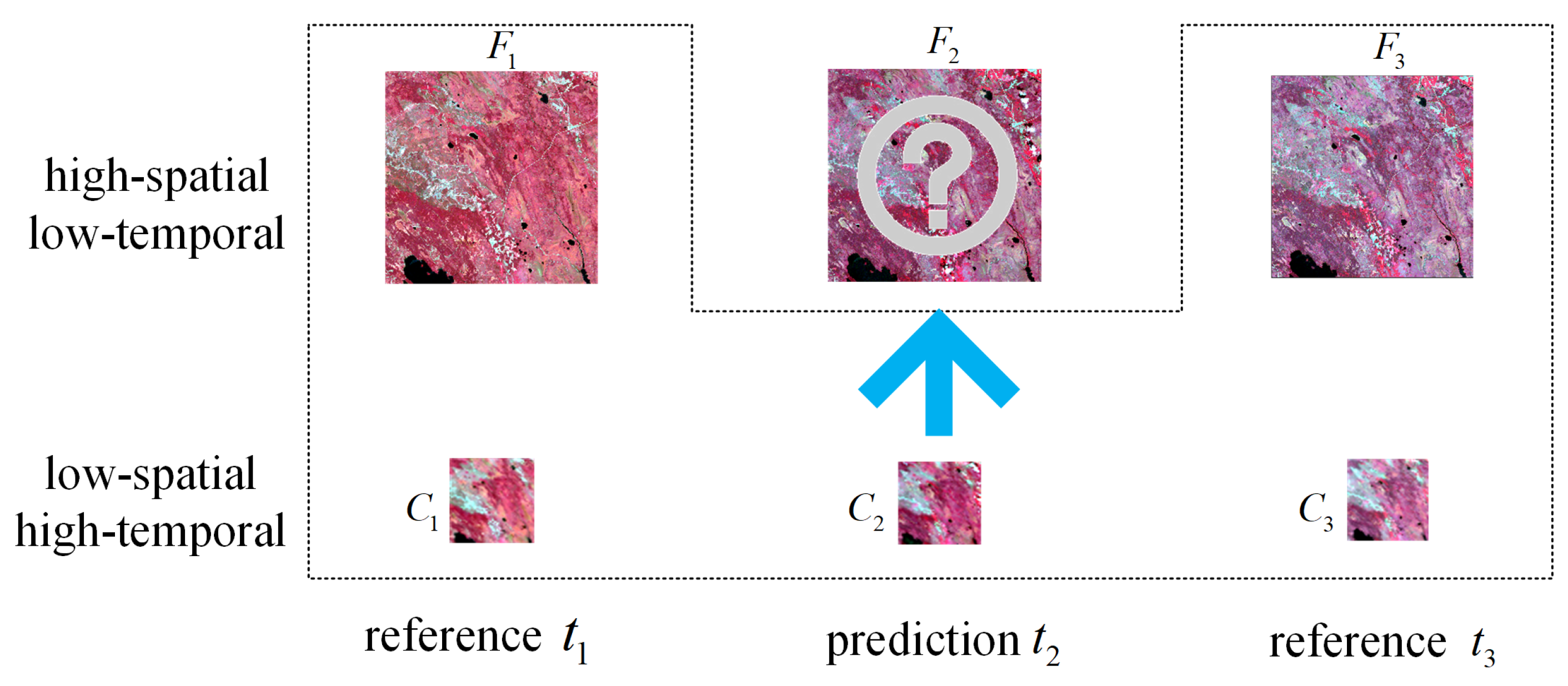
Spatiotemporal fusion consists of two types of remote sensing images, as shown in Figure 1. One type has high temporal and low spatial resolutions (hereinafter referred to as low-resolution or coarse-resolution images). The other type has high spatial and low temporal resolution (hereinafter referred to as high-resolution or fine-resolution images). The spatiotemporal fusion is to predict the missing high-resolution image on the prediction date $t_2$ by utilizing the low-resolution image at $t_2$ and at least one pair of high- and low-resolution images for reference at $t_i$ (where $i\ne 2$).

Existing spatiotemporal fusion methods can be categorized as weight-based, unmixing-based, learning-based, and hybrid methods. Weight-function-based methods apply a linear model to multi-source observations of pure coarse-resolution pixels, and further utilize a weighting strategy to enhance predictions for mixed pixels. These methods exploit the spatial dependence of spectrally similar pixels to reduce the uncertainty and block artifacts in fusion results. The fusion is performed locally, which leads to fast and linear processing speeds. Besides the classic STARFM algorithm [3], enhanced STARFM [16], linear injection [22], and Fit-FC [23] are also typical weight-based methods. However, strategies that relies solely only on pixel similarity fail to maintain structure and detail, so that complex regions require higher coarse image resolution.

Following the framework proposed by Zhukov et al. [24], unmixing-based methods [25,26,27,28] employ spatial unmixing techniques for fusion, which estimate the high-resolution endmembers by unmixing the coarse-resolution pixels using the class scores explained by the reference image. Due to the wide spectrum and large resolution ratio, the unmixing-based methods may be prone to errors in abundance estimation, spectral variations, and nonlinear mixing.

Learning-based methods take advantage of recent advances in machine learning [29] to model the relationship between inputs and outputs, which include dictionary learning, extreme learning machine, random forest, Bayesian framework, and convolutional neural networks. The dictionary-pair-based algorithms [30,31,32,33] use sparse representation to establish connections between high- and low-resolution images. Deep neural networks have replaced them for learning large volumes of data more efficiently. Using complex network structures, neural network learning has the potential to map spatial, temporal, and sensor relationships between images from different sources, as have been proposed for spatiotemporal fusion [6,20,34,35,36,37]. These methods have significant modeling advantages, but suffer from the quality and size of the training data. Low-quality data will train worse nonlinear relationships than dictionary learning. The fusion effect of inadequate training may also be inferior to that of traditional weight or unmixed based models. Therefore, neural network methods are not easily used for the spatiotemporal fusion of one pair.

Hybrid methods combine the advantages of diverse categories to pursue better performance. The flexible spatiotemporal data fusion (FSDAF) algorithm is an important representative that harnesses weight and unmixing for spatiotemporal fusion. Its revisions, such as SFSDAF [38], FSDAF 2.0 [39], and EFSDAF [40], can also be categorized into this type. Other hybrid studies [28,41] integrated weight and unmixing strategies, too. Our previous work [42] is also a hybrid type, which integrates the results of FSDAF and Fit-FC to enhance performance.

A typical spatiotemporal fusion uses three images, but a few studies have attempted to reduce the number of input images to two. Fung et al. [43] utilized the optimization concept in the Hopfield neural network for spatiotemporal image fusion and proposed a new algorithm named the Hopfield neural network Spatio-temporal data fusion model (HNN-SPOT). The algorithm uses a fine-resolution image taken on an arbitrary date and a coarse image taken on the forecast date to derive a synthesized fine-resolution image of the forecast date. Subsequently, Wu et al. [44] also achieved data fusion only using the other two images as input. They proposed an efficient fusion strategy that degenerates the high-resolution images of the reference date to obtain simulated low-resolution images, which can be combined with any spatiotemporal fusion model to accomplish the fusion with simplified input. On the three spatiotemporal fusion algorithms of STARFM, STNLFFM, and FSDAF, experiments were carried out on the datasets of MODIS, Landsat, and Sentinel-2 land surface reflectance product, and the results suggest that the fusion performance with only two input images is comparable to or even superior than that of three input images. Tan et al. [36] proposed the GAN-based spatiotemporal fusion model (GAN-STFM) with a conditional generative adversarial network to reduce the number of model inputs free of the time restriction on reference image selection. Liu et al. [45] presented a GAN survey for remote sensing fusion.

Some algorithms focus on improving the fusion speed of spatiotemporal fusion. Li et al. [46] proposed an extremely fast spatiotemporal fusion method with local normalization to extract spatial information from the prior high-spatial-resolution images and embeds that information into the low-spatial-resolution images in order to predict the missing high-spatial-resolution images. Gao et al. [47] proposed an enhanced FSDAF (cuFSDAF) with GPUs of different computing capabilities to process datasets of arbitrary size.

It is well-known that the performance of spatiotemporal fusion algorithms is unstable. Therefore, several studies have analyzed the impact of factors such as time interval, registration error, number of bands, and clouds. The experiment conducted by Shao et al. [48] originating from an enhanced super-resolution convolutional neural network demonstrated that the number of input auxiliary images and the temporal interval (i.e., the difference between image acquisition dates) between the auxiliary images and the target image both influence the performance of the fusion network. Tang and Wang [49] analyzed the influence of geometric registration errors on spatiotemporal fusion. Subsequently, Wang et al. [50] studied the effect of registration errors on patch-based spatiotemporal fusion methods. Experimental results show that the patch-based fusion model SPSTFM is more robust and accurate than pixel-based fusion models (such as STARFM and Fit-FC), and for each method, the effect of the registration error is greater for heterogeneous regions than for homogeneous regions. Tan et al. [6] proposed an enhanced deep convolutional spatiotemporal fusion network (EDCSTFN) and found that multiband deep learning models slightly outperform single-band deep learning models. Luo et al. [51] proposed a generic and fully automated method (STAIR) for spatiotemporal fusion to impute the missing-value pixels due to cloud cover or sensor mechanical issues in satellite images using an adaptive-average correction process to generate cloud- or gap-free data.

Spatiotemporal fusion has the potential to construct results whose resolution exceeds that of high-resolution reference images. Chen and Xu [52] proposed a unified spatial–temporal–spectral blending model to improve the utilization of accessible satellite data. First, an improved adaptive intensity–hue–saturation approach was used to enhance the spatial resolution of Landsat Enhanced Thematic Mapper Plus (ETM+) data; then, STARFM was used to fuse the MODIS and enhanced Landsat ETM+ data to generate the final synthetic data. Wei et al. [53] fused 8-m multispectral images with 16-m wide-field-view images to reduce the revisiting time of the 8-m multispectral images to 4 days from the original 49 days. The fused results are further improved to 2 m using the panchromatic band.

The data used for spatiotemporal fusion are largely either the Landsat series or MODIS data, but spatiotemporal fusion for other satellites is also being explored, too. For example, Rao et al. [54] conducted spatiotemporal fusion of the LISS sensor (23.5 m with a 24-day revisiting period) and the AWiFS sensor (56 m and a revisiting period of 5 days) on the Indian satellite Resourcesat-2 to obtain synthetic data with a ground resolution of 23.5 m and a revisiting period of 5 days. Similar studies were performed between Sentinel-3 and Sentinel-2 [23], SPOT5 and MODIS [55], Landsat Thematic Mapper (TM) and Envisat Medium Resolution Imaging Spectrometer (MERIS) [56], Planet and Worldview [57], and the multispectral sensors within Gaofen-1 [53].

Although the performance of spatiotemporal fusion algorithms is far from perfect, they have been put to practice. For example, Ding et al. [18] used the fusion results to extract rice fields. Xin et al. [58] used the fusion results to improve the near-real-time monitoring of forest disturbances. Zhang et al. [59] utilized the NDVI data obtained via spatiotemporal fusion to establish a grassland biomass estimation model for monitoring seasonal vegetable changes. In terms of water applications, Guo et al. [60] proposed a spatiotemporal fusion model to monitor marine ecology through chlorophyll-a inversion. In addition to conventional remote sensing applications, spatiotemporal fusion is also applied to synthesize surface brightness temperature data [19,61]. Shi et al. [62] proposed a comprehensive FSDAF (CFSDAF) method to observe the land surface temperature in urban areas with high spatial and temporal resolutions.

3. Preparation for Comparison

3.1. Datasets

Most spatiotemporal fusion studies were conducted between the Landsat series and MODIS Terra. Both are in sun-synchronous orbits at an altitude of 705 km and captured between 10:00 a.m. and 10:30 a.m. local time. The spectral response curves of commonly used data sources are shown in Figure 2. The mean absolute deviations between MODIS and Landsat-5, Landsat-7, and Landsat-8 are 0.1704, 0.1524, and 0.3301, respectively.

Four Landsat datasets have been prepared for the experiment and comparisons. All Landsat images are the product of surface reflectance obtained after atmospheric correction. The pixel values are then magnified by a factor of 10,000 and quantized with 16-bit integers so that they fall within the theoretical range of 0 to 10,000. Besides the Landsat-7 and Landsat-8 sources, we also tested a time-series FY4ASRcolor dataset from the FY4A Meteorological Satellite. The FY4ASRcolor images are from two separate cameras of the same satellite. The summaries of all the datasets are given in

Table 1. Summary of the datasets.

	Columns *	Rows *	Bands	Amount	Location
L7STARFM	1200	1200	green, red, NIR	3	Canada (104${}^{°}$W, 54${}^{°}$N)
CIA	1408	1824	blue, green, red, NIR	17	Australia (34.0034${}^{°}$E, 145.0675${}^{°}$S)
LGC	3184	2704	blue green, red, NIR	14	Australia (149.2815${}^{°}$E, 286 29.0855${}^{°}$S)
L8JX	5792	5488	blue, green, red, NIR	9	China (115.8247${}^{°}$E, 25.9868${}^{°}$N)
FY4ASRcolor	10,992	4368	blue, red–green, VNIR	165	whole China

* The columns and rows of CIA and LGC are smaller than the original sizes after the black borders are removed.

and will be detailed as follows.

3.1.1. L7STARFM

L7STARFM contains three pairs of Landsat-7 ETM+ and MODIS images that were captured on 24 May 2001; 11 July 2001; and 12 August 2001, respectively. All images consist of green, red, and near-infrared bands that are derived from the surface reflectance products. The image sizes are 1200 × 1200. The ground resolution of Landsat-7 images is 30 m, while it is 500 m for MODIS. The data were first used in STARFM [3] and have been tested in numerous works for traditional one-pair algorithms including weight-based, unmixing-based, and dictionary-learning-based methods, which have no complex architectures for training; therefore, the dataset is named L7STARFM. The dataset is available at https://github.com/isstncu/l8jx (accessed on 20 July 2023).

3.1.2. CIA

The CIA dataset [17] is widely used to benchmark spatiotemporal fusion algorithms. Seventeen cloud-free Landsat7 ETM+ to MODIS image pairs were captured between October 2001 and May 2002, a time when crop phenology has significant temporal dynamics. Geographically, the area covered by the CIA dataset is the Coleambally Irrigation Area (CIA) in southern New South Wales, Australia (34.0034${}^{°}$E, 145.0675${}^{°}$S). Each image spans 43 km from north to south and 51 km from east to west. The total area is 2193 km${}^2$ and consists of 1720 columns and 2040 rows at a ground resolution of 25 m. Each image consists of six bands. The dataset is available at https://data.csiro.au/collection/csiro:5846v1 (accessed on 20 July 2023).

In the test, the blue, green, red, and near-infrared (NIR) bands of CIA images are used, and the image size is reduced to 1408 columns and 1824 rows by removing the blank areas outside the valid image scope. The blank areas are cropped because the algorithms do not account for invalid data during processing, which may result in significant errors in training and reconstruction. The neural-network-based algorithms require a large amount of data for training. Therefore, the training data come from the 10 images in 2002, while the validation dataset comprises 5 images from 2001. Other algorithms can perform one-pair spatiotemporal fusion, in which the reference times are 5 January 2002; 13 February 2002; 11 April 2002; 18 April 2002; and 18 April 2002, respectively, and the prediction times are 4 December 2001; 2 November 2001; 17 October 2001; 9 November 2001; and 25 November 2001, respectively.

Other algorithms can perform one-pair spatiotemporal fusion, in which the reference time is 5 January 2002, 13 February 2002, 11 April 2002, 18 April 2002, and 18 April 2002, respectively, and the prediction time is 4 December 2001, 2 November 2001, 17 October 2001, 9 November 2001, and 25 November 2001, respectively.

3.1.3. LGC

The Lower Gwydir Catchment (LGC) study site [17] is located in northern New South Wales, Australia (149.2815${}^{°}$E, 29.0855${}^{°}$S). Fourteen cloud-free Landsat Thematic Mapper (TM) and MODIS image pairs across the LGC were taken from April 2004 to April 2005. The LGC dataset spans the Gwidir river with a width of 80 km from north to south and 68 km from east to west and an total area of 5440 km${}^2$. The images have 3200 columns and 2720 rows with a ground resolution of 25 m. LGC experienced severe flooding in mid-December 2004, resulting in approximately 44% of the area being submerged. Due to the different spatial and temporal changes caused by flood events, the LGC dataset can be considered a dynamically changing site. The dataset is available at https://data.csiro.au/collection/csiro:5847v1 (accessed on 20 July 2023).

Similar to the CIA dataset, the blue, green, red, and NIR bands of the LGC dataset are extracted after removing the outer blank areas within the images, so 3184 columns and 2704 rows remain. When used for neural network evaluation, the nine images from 2004 are used for training, while the four images from 2001 are to be reconstructed. The dates to be reconstructed are set as follows: 3 April 2005; 2 March 2005; 13 January 2005; and 29 January 2005. Other algorithms use one-pair fusion, where the corresponding reference images are 2 May 2004; 26 November 2004; 28 December 2004; and 28 December 2004.

3.1.4. L8JX

The L8JX dataset is designed by us to test the availability of neural networks for one-pair spatiotemporal fusion. Landsat-8 OLI images were captured in December 2017, October 2018, and November 2017, respectively. The corresponding low-resolution images are the synthesized 8-day MODIS MOD09A1 products. Each image has the blue, green, red, and NIR bands. According to the grid rule of Landsat satellites, these images cover Jiangxi Province in China. The path numbers are 121, and the row numbers are 41, 42, and 43, respectively. The dataset is given the name L8JX for abbreviation, which has 9 pairs of images.

Due to the tilt of the orbit, there are black borders around the image content. In order to remove the useless space in the images, additional processing was carried. The original Landsat-8 images were rotated counterclockwise by approximately 13 degrees, and then the common areas without black borders were extracted. The entire dataset was then divided into three scenes that are geographically connected through small overlapping areas, which can be used as the ground truth to benchmark spatiotemporal fusion or mosaicking algorithms. Each image in L8JX has 5792 columns and 5488 rows. The 8-day MODIS images were rotated, and the blank areas were also removed at the same time. The dataset is available at https://github.com/isstncu/l8jx (accessed on 20 July 2023).

3.1.5. FY4ASRcolor

The FY4ASRcolor dataset [21] is proposed for testing the super resolution of low-resolution remote sensing images. The FY4ASRcolor dataset spans the blue (450–490 nm), red–green (550–750 nm), and visible near-infrared (VNIR, 750–900 nm) bands. The ground resolutions are 1 km for the high-resolution part and 4 km for the low-resolution part. Images in the dataset were captured on 16 September 2021. Each image in L8JX has 10,992 columns and 4368 rows. All the bands are in a 16-bit data format with 12-bit quantization, meaning that each digital number ranges from 0 to 4095. The dataset is available at https://github.com/isstncu/fy4a (accessed on 20 July 2023).

FY4ASRcolor can be used to test spatiotemporal fusion because it comprises time-series data. The images in FY4ASRcolor are all captured by the Advanced Geostationary Radiation Imager (AGRI) camera with full disc scanning covering China (region of China, REGC) with a 5-min time interval for regional scanning. Because of the continuous change in solar angle, the radiation values can change dramatically over large time intervals. Since the daily radiative variation is repetitive, the spatiotemporal fusion of FY4ASRcolor can be used to assess the feasibility of learning the variation pattern throughout a year.

The FY4ASRcolor dataset gives another chance of spatiotemporal fusion within homogeneous platforms instead of heterogenous platforms. The high- and low-resolution images in FY4ASRcolor are acquired by separately mounted sensors of the same type. Different from MODIS and Landsat, each pair of images in the FY4ASRcolor dataset was taken simultaneously using the same sensor response. The sensor difference in FY4ASRcolor is much smaller compared to the L7STARFM, CIA, LGC, and L8JX datasets, as the average absolute error is 29.63. Usually, the sensor difference is hardly modeled, as it is stochastic and scene-dependent. The minimal sensor difference in the FY4ASRcolor dataset makes it ideal for conducting spatiotemporal fusion studies, as it eliminates the fatal sensor discrepancy issue in fusing MODIS and Landsat. A similar work was carried out by us for the spatiotemporal–spectral fusion of the Gaofen-1 images [53]. However, there is only a 2-fold difference in spatial resolution.

3.2. Methods

Fourteen spatiotemporal fusion algorithms covering three categories are collected for evaluation. These algorithms include STARFM [3], Fit-FC [3], VIPSTF [63], FSDAF [4], SFSDAF [38], SPSTFM [30], EBSCDL [31], CSSF [33], BiaSTF [34], DMNet [35], EDCSTFN [6], GANSTFM [36], MOST [20], and SSTSTF [37].

STARFM, Fit-FC, and VIPSTF-SW are weight-based methods. STARFM is a classic and widely used spatiotemporal fusion approach. Fit-FC addresses the problem of discontinuities caused by clouds or shadows in spatiotemporal fusion. VIPSTF is a flexible framework with two versions, VIPSTF-SW and VIPSTF-SU, where the weight-based version (VIPSTF-SW) will be used and abbreviated as VIPSTF. VIPSTF produced the concept of a virtual image pair (VIP), which makes use of the observed image pairs to reduce the uncertainty of estimating the increment from fine-resolution images.

FSDAF and SFSDAF are hybrid methods. FSDAF is a spatiotemporal fusion framework that is compatible with both slow and abrupt changes in land surface reflectance and automatically predicts both gradual and land cover changes through an error analysis in the fusion process. SFSDAF is an enhanced FSDAF framework that aims to reconstruct heterogeneous regions undergoing land cover changes. It utilizes sub-pixel class fraction change information to make inferences.

SPSTFM, EBSCDL, and CSSF are dictionary-learning-based methods. SPSTFM trains two dictionaries generated from coarse- and fine-resolution difference image patches at the given time to build the coupled dictionaries for reconstruction. EBSCDL fixed the dictionary perturbations in SPSTFM using the error-bound-regularized method, which leads to a semi-coupled dictionary pair to address the differences between the coarse- and fine-resolution images. Compressed sensing for spatiotemporal fusion is addressed in CSSF, which explicitly describes the downsampling process and solves it using the dual semi-coupled dictionary pairs.

In the comparison methods, STARFM, BiaSTF, DMNet, EDCSTFN, GANSTFM, MOST, and SSTSTF are coded with Python. The PyTorch framework is used for deep learning. Fit-FC, VIPSTF, SFSDAF, SPSTFM, EBSCDL, and CSSF are coded with MATLAB. FSDAF is coded with Interactive Data Language (IDL). All hyperparameters are set according to the original articles. The experimental conditions are presented in

Table 2. Hardware and software for experiments.

Hardware	RAM	CPU	GPU
	128GB	Intel Xeon E5-2682 v4 @ 2.50GHz	nVidia Tesla V100
Software	Python	CUDA	PyTorch
	3.6.2	10.2	1.2.0

.

BiaSTF, DMNet, EDCSTFN, GANSTF, MOST, and SSTSTF use convolutional neural networks for fusion. BiaSTF models the sensor differences as a bias, which is modeled with convolutional neural networks to alleviate the spectral and spatial distortions in reconstructed images. DMNet introduces multiscale mechanisms and dilated convolutions to capture more abundant details while reducing the number of trainable parameters. EDCSTFN is an enhanced deep convolutional spatiotemporal fusion network with convolutional neural networks used to extract details of high-resolution images and residuals between all known images. GANSTF introduces the conditional generative adversarial network and switchable normalization technique into the spatiotemporal fusion problem, where the low-resolution images at the given time are not needed. MOST cascades enhanced deep neural networks and trains the spatial and sensor differences separately to fuse images quickly and effectively. SSTSTF proposes a step-by-step modeling framework, and three models have been designed based on deep neural networks to explicitly model the spatial difference, sensor difference, and temporal difference separately. In the training stage, BiaSTF, DMNet, MOST, and SSTSTF can be trained with only one pair, while EDCSTFN and GANSTF need two or more pairs to learn temporal changes. Training parameters are given in

Table 3. Parameters for CNN training.

Algorithm	Optimizer	Initial Learning Rate	Epochs	Batch Size	Patch Size	Training Time (s)
BiaSTF	Adam	0.0001	300	64	128 × 128	10,647
DMNet	Adam	0.001	60	32	60 × 60	15,609
EDCSTFN	Adam	0.0001	60	36	256 × 256	3036
GANSTFM	Adam	0.0002	300	32	256 × 256	18,445
MOST	Adam	0.0001	300	16	54 × 54	18,566
SSTSTF	Adam	0.0001	300	36	256 × 256	25,427

for CNN-based algorithms, where the average training time is also given by training the first band of the L8JX dataset twice.

3.3. Metrics

Metrics are also used to assess the performance of the synthesized images. Root mean square error (RMSE) measures the radiometric discrepancy. Spectral angle mapper (SAM), relative average spectral error (RASE) [64], relative dimensionless global error in synthesis (ERGAS) [65], and Q4 [66] measure the color consistency. Three metrics are used to measure the structural similarity, including the classic structural similarity (SSIM), the normalized difference Robert’s edge (ndEdge) for edge similarity, and the normalized difference local binary pattern (ndLBP) for textural similarity. To help readers understand the digital trends, the negative SSIM (nSSIM) and negative Q4 (nQ4) are used instead of the standard definitions.

To establish the metrics, the LandSat images taken at a specific time are used as the ground truth. To evaluate the spectral consistency with SAM, RASE, ERGAS, and nQ4, the NIR, red, and green bands are used, but not the blue band. The ideal results are 0 for all the metrics.

RMSE is calculated as

$$\mathrm{RMSE}=\sqrt{\frac{1}{N}{\sum }_{i=1}^N{\left(x_i-y_i\right)}^2}$$

(1)

where x and y are two single-band images sharing the same pixel quantity N, and i is a pixel location.

For a reference image x and an evaluation image y, the spectral angle SAM metric between y and x is calculated using the normalized correlated coefficient as follows:

$$\mathrm{SAM}=arccos\left(\frac{〈x,y〉}{∥x∥∥y∥}\right)$$

(2)

where $〈x,y〉$ is the inner product between x and y.

For a reference image x and an evaluation image y, the RASE metric for y to reference x is calculated as

$$\mathrm{RASE}=\frac{\mathrm{RMSE}\left(x-y\right)}{\overline{x}}=\sqrt{\frac{1}{N·C}{\sum }_{i=1}^{N·C}{\left(x_i-y_i\right)}^2}/\overline{x}$$

(3)

where RMSE is the root mean square error between two images (calculated using pixels in all bands), N is the number of pixel locations (product of the width and height), and C is the number of bands.

The ERGAS metric is calculated as

$$\mathrm{ERGAS}=\frac{1}{r}\sqrt{\frac{1}{C}{\sum }_{c=1}^C\frac{RMSE{\left(x_c-y_c\right)}^2}{{{\overline{x}}_c}^2}}$$

(4)

where C is the number of total bands in an image, $x_c$ is the $c^{th}$ band of image x, $y_c$ is the $c^{th}$ band of image y, and ${\overline{x}}_c$ is the mean value of $x_c$. r is the resolution ratio between high- and low-resolution images which is initially defined for pansharpening. For example, r is set to 2 to evaluate the LandSat-7 fusion between the 15m panchromatic band and the 30 m multispectral bands. For hyperspectral visualization, r is set to 1.

Q4 is defined by

$$\mathrm{Q}4=\frac{4·\left|\mathrm{cov}\left({\mathbf{z}}_x,{\mathbf{z}}_y\right)\right|·\left|{\overline{\mathbf{z}}}_x\right|·\left|{\overline{\mathbf{z}}}_y\right|}{\left[\mathrm{cov}\left({\mathbf{z}}_x,{\mathbf{z}}_x\right)+\mathrm{cov}\left({\mathbf{z}}_y,{\mathbf{z}}_y\right)\right]\left({\left|{\overline{\mathbf{z}}}_x\right|}^2+{\left|{\overline{\mathbf{z}}}_y\right|}^y\right)}$$

(5)

where two quaternion variables are defined as

$${\mathbf{z}}_x=a_x+\mathrm{i}·b_x+\mathrm{j}·c_x+\mathrm{k}·d_x$$

(6)

$${\mathbf{z}}_y=a_y+\mathrm{i}·b_y+\mathrm{j}·c_y+\mathrm{k}·d_y$$

(7)

where $\mathrm{i}$, $\mathrm{j}$, and $\mathrm{k}$ are basic notations of a quaternion.

For a color image x, $a_x$ is 0, and $b_x$, $c_x$, and $d_x$ correspond in turn to pixel values of the three bands. This forms a column vector of quaternions. Analogously, $a_y$ is 0, and $b_y$, $c_y$, and $d_y$ correspond in turn to pixel values of the three bands of the image y. ${\overline{\mathbf{z}}}_x$ and ${\overline{\mathbf{z}}}_y$ are the mean values of quaternion vectors ${\mathbf{z}}_x$ and ${\mathbf{z}}_y$, respectively.

For a quaternion notation $z=a+\mathrm{i}b+\mathrm{j}c+\mathrm{k}d$, the modulus $\left|\overline{z}\right|$ is calculated using

$$\left|z\right|=\left|z·z^{*}\right|=\sqrt{a^2+b^2+c^2+d^2}$$

(8)

where $z^{*}$ is the conjugate of z and defined by

$$z^{*}=a-\mathrm{i}b-\mathrm{j}c-\mathrm{k}d.$$

(9)

The covariance between quaternion vectors ${\mathbf{z}}_x$ and ${\mathbf{z}}_y$ is

$$\mathrm{cov}\left({\mathbf{z}}_x,{\mathbf{z}}_y\right)=\frac{{\left({\mathbf{z}}_x-{\overline{\mathbf{z}}}_x\right)}^T{\left({\mathbf{z}}_y-{\overline{\mathbf{z}}}_y\right)}^{*}}{N}.$$

(10)

Instead of the standard Q4 index, the negative Q4 (nQ4) is used, which is defined as

$$\mathrm{nQ}4=1-\mathrm{Q}4$$

(11)

nSSIM is calculated using

$$\begin{array}{cc}\hfill {\mathrm{SSIM}}_{x,y}& =\frac{\left(2{\mu }_x{\mu }_y+c_1\right)\left(2{\sigma }_{xy}+c_2\right)}{\left({\mu }_{{}_x}^2+{\mu }_{{}_y}^2+c_1\right)\left({\sigma }_{{}_x}^2+{\sigma }_{{}_y}^2+c_2\right)}\hfill \\ \hfill \mathrm{nSSIM}& =1-\mathrm{SSIM}\hfill \end{array}$$

(12)

where x and y are two single-band images, ${\mu }_x$ and ${\mu }_y$ denote the mean values, ${\sigma }_x$ and ${\sigma }_y$ denote the standard deviations, and ${\sigma }_{xy}$ is the covariance between x and y. $c_1$ and $c_2$ are small constants to avoid zeros.

Robert’s edge (Edge) is used to measure the edge features of fused images by detecting local discontinuities. For an image x, the edge discontinuity at the coordinate $(i,j)$ is defined as ${\mathrm{Edge}}_{i,j}$

$${\mathrm{Edge}}_{i,j}=\left|x_{i,j}-x_{i+1,j+1}\right|+\left|x_{i,j+1}-x_{i+1,j}\right|$$

(13)

where $x_{i,j}$ is the pixel value at the location $(i,j)$.

A Robert’s edge image is generated after the point-by-point calculation for the image x, which can be defined as ${\mathrm{Edge}}_x$. By denoting the Robert’s edge images for the fused image and the ground truth image as ${\mathrm{Edge}}_F$ and ${\mathrm{Edge}}_R$, respectively, the normalized difference Edge index ($\mathrm{ndEdge}$) between them is calculated as

$$\mathrm{ndEdge}=\frac{{\mathrm{Edge}}_F-{\mathrm{Edge}}_R}{{\mathrm{Edge}}_F+{\mathrm{Edge}}_R}$$

(14)

It should be noted that the ndEdge’s calculation involves only 10% of locations with higher Edge values which are determined from ${\mathrm{Edge}}_R$. For a multiband image, after finding the ndEdge of each band, the average of these values yields a total ndEdge.

The local binary pattern (LBP) is an operator that describes the local texture characteristics of an image. In a $3\times 3$ window, the center pixel is adjacent to 8 pixels. The adjacent locations are marked as 1 if their gray values are larger than that of the center pixel, and 0 otherwise. By concatenating the eight comparison results, an 8-bit binary digit is obtained ranging from 0 to 255, which we call the LBP code of the center pixel. The point-by-point calculation for each point gives an LBP image.

By denoting the LBP images for the fused image and the ground truth image as ${\mathrm{LBP}}_F$ and ${\mathrm{LBP}}_R$, respectively, the normalized difference LBP index ($\mathrm{ndEdge}$) between them is calculated as

$$\mathrm{ndLBP}=\frac{\mathrm{LBP}{}_F-\mathrm{LBP}{}_R}{\mathrm{LBP}{}_F+\mathrm{LBP}{}_R}$$

(15)

Similar to the calculation of multiband ndEdge, after finding the ndLBP for each band of a multiband image, the average of these values is the total ndLBP.

In order to present the radiometric error with a percentage indicator, the relative uncertainty is evaluated, which is defined as

$$\mathrm{uncertainty}=\frac{\mathrm{absolute}\mathrm{error}}{\mathrm{measured}\mathrm{value}}.$$

(16)

The mean relative uncertainty of a single-channel image is the mean value of relative uncertainty across all pixel locations. The best uncertainty is given to represent the optimal performance that the state-of-the-art algorithms can reach.

The mean value (mean) and correlated coefficient (CC) are also calculated. The mean value is an indicator for data range, and CC illustrates the similarity between the reference images and the target images.

4. Experimental Results for Spatiotemporal Fusion

All five datasets were tested using fourteen algorithms from three categories, and the results were evaluated using the RMSE, SAM, RASE, ERGAS, nQ4, nSSIM, ndEdge, and ndLBP. The scores are listed in

Table 4. RMSE evaluation on the CIA (LandSat-7) dataset.

target	4 December 2001				2 November 2001				17 October 2001				9 November 2001				25 November 2001
reference	5 January 2002				13 February 2002				11 April 2002				18 April 2002				18 April 2002
band	blue	green	red	NIR	blue	green	red	NIR	blue	green	red	NIR	blue	green	red	NIR	blue	green	red	NIR
mean	713	1069	1474	2550	507	783	988	2376	469	708	859	2431	439	724	971	2207	502	841	1203	2234
CC	0.822	0.805	0.861	0.393	0.413	0.435	0.406	−0.418	0.231	0.262	0.249	−0.210	0.382	0.310	0.330	−0.172	0.446	0.334	0.315	−0.149
STARFM	125.7	186.5	293.4	526.3	175.1	221.8	362.1	913.7	169.8	200.3	324.5	846.9	86.3	115.2	189.9	465.2	151.5	203.5	345.0	624.4
Fit-FC	101.0	145.5	223.5	457.9	131.0	170.4	261.6	562.7	148.3	187.0	284.7	671.2	119.9	162.3	247.5	556.3	136.7	187.0	296.1	473.2
VIPSTF	120.3	176.1	223.2	464.0	162.7	207.9	292.1	613.3	168.3	203.1	312.2	711.6	144.1	194.5	286.8	583.6	157.6	225.6	346.7	491.1
FSDAF	114.5	168.3	256.5	481.0	162.4	205.6	328.1	825.4	173.2	200.9	319.9	856.2	143.1	179.5	287.1	704.0	146.8	198.4	328.7	621.7
SFSDAF	117.5	171.8	269.2	482.5	160.0	202.6	320.9	823.6	173.6	201.7	316.3	854.6	146.4	184.4	292.4	708.4	152.5	203.8	335.4	627.5
SPSTFM	156.4	239.1	366.1	733.4	234.2	301.8	497.5	1260.6	208.4	248.4	419.4	1172.2	183.0	240.3	391.1	992.8	175.9	250.8	427.8	899.1
EBSCDL	136.9	204.8	315.4	604.6	188.9	241.0	392.1	1080.7	178.2	209.0	340.4	1003.0	153.1	197.5	315.2	837.1	154.7	214.4	357.1	748.9
CSSF	139.3	208.5	321.8	602.2	195.4	249.5	408.8	1091.9	184.8	217.1	354.0	1025.9	156.5	203.5	325.2	869.9	158.0	221.2	371.0	774.3
BiaSTF	138.5	207.7	317.7	584.3	192.0	238.4	384.8	1032.0	197.9	229.5	349.1	971.0	152.2	196.5	312.0	820.6	165.6	220.9	359.2	737.7
DMNet	120.8	167.2	256.7	544.9	170.1	211.4	376.3	940.3	156.2	206.8	330.6	909.2	140.1	180.3	294.0	769.4	154.1	212.9	345.9	682.9
EDCSTFN	121.3	185.1	263.2	764.8	201.3	239.1	418.8	1245.6	164.2	205.1	363.8	985.6	141.3	184.6	315.9	823.8	149.0	213.0	388.2	748.8
GANSTFM	142.6	187.0	275.0	539.3	169.8	197.4	303.7	893.0	184.8	200.5	330.6	908.1	135.2	170.2	268.2	738.1	131.4	180.3	313.2	617.5
MOST	123.7	163.4	253.6	571.6	164.8	209.7	342.6	802.8	193.0	220.0	377.5	957.8	143.6	184.8	298.0	733.6	146.1	201.1	341.0	671.1
SSTSTF	129.0	182.4	291.3	530.6	138.9	178.2	291.7	827.5	154.1	193.5	298.7	851.6	124.6	162.5	256.0	670.6	158.6	211.3	323.4	551.8
uncertainty *(%)	11.0	10.8	12.6	15.7	20.4	17.6	25.5	24.4	22.2	18.9	31.1	25.9	18.2	13.9	18.9	20.3	24.3	17.5	25.0	19.8

* The uncertainty values are the lowest values across all fusion results.

,

Table 5. Spectral Consistency Evaluation on the CIA (LandSat-7) Dataset.

target	3 December 2001				1 November 2001				16 October 2001				8 November 2001				24 November 2001
reference	4 January 2002				12 February 2002				10 April 2002				17 April 2002				17 April 2002
metric	SAM	RASE	ERGAS	nQ4	SAM	RASE	ERGAS	nQ4	SAM	RASE	ERGAS	nQ4	SAM	RASE	ERGAS	nQ4	SAM	RASE	ERGAS	nQ4
STARFM	0.083	0.215	0.194	0.216	0.184	0.421	0.348	0.655	0.133	0.402	0.339	0.635	0.127	0.229	0.190	0.162	0.085	0.300	0.270	0.593
Fit-FC	0.052	0.180	0.157	0.218	0.100	0.269	0.241	0.337	0.114	0.326	0.292	0.454	0.090	0.280	0.244	0.436	0.067	0.238	0.227	0.427
VIPSTF	0.069	0.185	0.167	0.209	0.130	0.297	0.274	0.437	0.127	0.348	0.316	0.561	0.100	0.301	0.276	0.532	0.082	0.260	0.260	0.526
FSDAF	0.070	0.194	0.174	0.188	0.166	0.381	0.316	0.614	0.135	0.405	0.338	0.647	0.110	0.347	0.289	0.606	0.084	0.296	0.263	0.585
SFSDAF	0.068	0.197	0.178	0.204	0.164	0.379	0.312	0.610	0.135	0.404	0.337	0.626	0.112	0.350	0.294	0.590	0.086	0.300	0.268	0.573
SPSTFM	0.110	0.290	0.255	0.286	0.249	0.580	0.477	0.644	0.190	0.550	0.445	0.850	0.152	0.485	0.398	0.965	0.118	0.416	0.355	0.904
EBSCDL	0.088	0.242	0.215	0.242	0.208	0.491	0.391	0.739	0.152	0.468	0.372	0.772	0.126	0.407	0.328	0.728	0.100	0.347	0.297	0.686
CSSF	0.093	0.243	0.217	0.245	0.218	0.498	0.402	0.728	0.157	0.479	0.384	0.812	0.130	0.422	0.340	0.796	0.103	0.359	0.308	0.750
BiaSTF	0.093	0.237	0.213	0.244	0.209	0.471	0.380	0.721	0.153	0.458	0.378	0.697	0.127	0.399	0.324	0.685	0.101	0.344	0.298	0.656
DMNet	0.075	0.213	0.183	0.223	0.186	0.432	0.353	0.695	0.143	0.429	0.353	0.764	0.113	0.374	0.303	0.736	0.091	0.322	0.283	0.716
EDCSTFN	0.083	0.282	0.225	0.286	0.243	0.558	0.427	0.643	0.169	0.464	0.377	0.859	0.131	0.400	0.322	0.808	0.108	0.352	0.306	0.809
GANSTFM	0.063	0.215	0.192	0.299	0.158	0.402	0.316	0.764	0.163	0.428	0.350	0.735	0.119	0.357	0.285	0.689	0.078	0.290	0.252	0.632
MOST	0.059	0.220	0.185	0.302	0.159	0.375	0.319	0.617	0.180	0.456	0.385	0.783	0.128	0.361	0.300	0.637	0.090	0.315	0.276	0.608
SSTSTF	0.058	0.215	0.193	0.301	0.144	0.374	0.295	0.583	0.138	0.400	0.326	0.541	0.102	0.327	0.266	0.507	0.072	0.273	0.256	0.469

,

Table 6. Average nSSIM/ndEdge/ndLBP evaluation on the CIA (LandSat-7) dataset.

target	3 December 2001			1 November 2001			16 October 2001			8 November 2001			24 November 2001
reference	4 January 2002			12 February 2002			10 April 2002			17 April 2002			17 April 2002
metric	nSSIM	ndEdge	ndLBP	nSSIM	ndEdge	ndLBP	nSSIM	ndEdge	ndLBP	nSSIM	ndEdge	ndLBP	nSSIM	ndEdge	ndLBP
STARFM	0.299	0.298	−0.036	0.691	0.345	−0.040	0.708	0.396	−0.064	0.161	0.166	−0.077	0.659	0.388	−0.056
Fit−FC	0.276	0.094	−0.069	0.591	0.172	−0.063	0.658	0.299	−0.070	0.629	0.292	−0.066	0.607	0.315	−0.061
VIPSTF	0.283	0.141	−0.068	0.716	0.130	−0.067	0.797	0.185	−0.069	0.752	0.288	−0.063	0.722	0.302	−0.059
FSDAF	0.232	0.262	−0.078	0.646	0.328	−0.079	0.709	0.370	−0.085	0.677	0.382	−0.080	0.645	0.369	−0.075
SFSDAF	0.257	0.296	−0.077	0.642	0.345	−0.080	0.704	0.383	−0.086	0.675	0.412	−0.083	0.647	0.397	−0.078
SPSTFM	0.298	0.302	−0.064	0.788	0.332	−0.059	0.853	0.366	−0.069	0.813	0.391	−0.065	0.774	0.373	−0.060
EBSCDL	0.288	0.298	−0.079	0.715	0.323	−0.080	0.747	0.359	−0.087	0.716	0.385	−0.080	0.684	0.365	−0.076
CSSF	0.289	0.297	−0.052	0.747	0.323	−0.048	0.792	0.360	−0.051	0.760	0.384	−0.045	0.730	0.364	−0.040
BiaSTF	0.294	0.297	−0.079	0.697	0.323	−0.080	0.727	0.360	−0.088	0.703	0.385	−0.083	0.671	0.366	−0.079
DMNet	0.272	0.121	−0.093	0.704	0.190	−0.100	0.759	0.213	−0.106	0.728	0.243	−0.100	0.705	0.237	−0.094
EDCSTFN	0.306	0.125	−0.094	0.768	0.186	−0.102	0.786	0.191	−0.109	0.739	0.220	−0.103	0.729	0.185	−0.097
GANSTFM	0.340	0.052	−0.086	0.695	0.181	−0.091	0.795	0.263	−0.097	0.694	0.268	−0.091	0.657	0.209	−0.085
MOST	0.316	0.079	−0.087	0.663	0.213	−0.096	0.839	0.249	−0.102	0.678	0.259	−0.096	0.615	0.238	−0.090
SSTSTF	0.367	0.087	−0.083	0.622	0.185	−0.090	0.668	0.259	−0.094	0.662	0.288	−0.088	0.626	0.255	−0.085

,

Table 7. RMSE evaluation on the LGC (LandSat-5) dataset.

target	3 April 2005				2 March 2005				13 January 2005				29 January 2005
reference	2 May 2004				26 November 2004				28 December 2004				28 December 2004
band	blue	green	red	NIR	blue	green	red	NIR	blue	green	red	NIR	blue	green	red	NIR
mean	702	1004	1224	2094	711	995	1185	2350	636	902	1005	2286	635	925	1023	2421
CC	0.576	0.535	0.538	0.362	0.500	0.463	0.431	0.452	0.759	0.781	0.800	0.806	0.739	0.744	0.759	0.688
STARFM	152.1	180.5	214.8	331.3	140.3	183.8	234.8	436.5	109.0	124.2	156.6	343.7	136.0	168.1	198.1	441.6
Fit-FC	171.1	188.4	203.2	316.3	166.4	178.8	219.3	425.7	116.6	114.9	143.8	293.9	140.4	161.8	192.2	420.5
VIPSTF	177.8	207.4	216.6	319.2	181.8	207.4	239.0	414.7	126.7	134.1	151.5	301.8	159.6	189.7	205.2	412.8
FSDAF	139.5	165.3	194.4	319.3	137.2	183.3	235.6	412.7	110.8	131.4	170.2	320.7	135.6	168.2	205.1	422.6
SFSDAF	143.8	171.7	200.7	328.5	137.9	183.8	235.6	412.7	105.0	126.7	163.0	348.3	131.8	166.5	199.8	442.1
SPSTFM	197.6	248.1	320.1	543.4	188.1	263.4	360.5	632.8	158.1	168.8	280.0	460.9	181.5	208.1	316.8	638.0
EBSCDL	151.4	183.0	222.1	384.5	144.8	194.4	249.4	470.6	123.2	139.1	172.8	330.5	144.1	172.8	204.0	457.6
CSSF	154.9	188.6	229.8	392.6	143.4	194.6	252.1	455.1	107.5	154.6	166.3	326.0	135.4	172.7	203.4	446.6
BiaSTF	144.8	179.9	222.2	375.7	148.0	191.4	242.9	432.8	101.4	119.0	160.8	329.8	125.5	156.2	195.6	437.1
DMNet	147.9	187.7	213.1	322.8	163.4	206.1	255.4	438.2	102.6	126.7	157.9	302.4	147.2	183.4	221.3	438.2
EDCSTFN	139.1	151.2	185.2	328.8	148.4	150.1	216.1	442.1	118.5	140.6	172.5	363.2	139.2	187.1	218.5	454.7
GANSTFM	122.6	157.0	173.8	282.4	110.2	135.3	196.8	379.5	89.3	109.2	164.5	337.6	121.9	157.3	196.3	426.7
MOST	128.7	151.7	177.6	297.3	117.1	137.5	195.0	366.8	95.6	109.1	177.8	333.4	125.5	152.8	191.7	430.3
SSTSTF	128.1	155.1	195.5	294.6	119.9	143.2	199.3	366.8	97.6	115.5	171.3	326.3	134.2	157.2	188.5	386.1
uncertainty *(%)	13.0	10.9	10.6	9.5	12.2	10.4	13.1	10.1	10.8	9.2	11.3	9.5	13.1	12.2	14.0	11.3

* The uncertainty values are the least values across all fusion results.

,

Table 8. Spectral Consistency Evaluation on the LGC (LandSat-5) Dataset.

target	3 April 2005				2 March 2005				13 January 2005				29 January 2005
reference	2 May 2004				26 November 2004				28 December 2004				28 December 2004
metric	SAM	RASE	ERGAS	nQ4	SAM	RASE	ERGAS	nQ4	SAM	RASE	ERGAS	nQ4	SAM	RASE	ERGAS	nQ4
STARFM	0.064	0.174	0.171	0.290	0.068	0.202	0.190	0.237	0.063	0.164	0.148	0.134	0.065	0.203	0.186	0.152
Fit-FC	0.063	0.169	0.169	0.271	0.071	0.195	0.182	0.223	0.062	0.143	0.133	0.096	0.066	0.194	0.179	0.139
VIPSTF	0.068	0.176	0.180	0.307	0.079	0.199	0.196	0.238	0.068	0.150	0.144	0.112	0.073	0.198	0.193	0.149
FSDAF	0.061	0.164	0.159	0.267	0.069	0.195	0.187	0.217	0.059	0.160	0.152	0.117	0.064	0.198	0.186	0.144
SFSDAF	0.063	0.169	0.164	0.276	0.068	0.195	0.187	0.218	0.063	0.167	0.152	0.127	0.066	0.203	0.186	0.152
SPSTFM	0.098	0.272	0.256	0.573	0.105	0.296	0.280	0.586	0.073	0.233	0.226	0.229	0.084	0.294	0.268	0.326
EBSCDL	0.072	0.192	0.182	0.320	0.069	0.217	0.202	0.267	0.063	0.164	0.157	0.120	0.068	0.210	0.192	0.158
CSSF	0.074	0.197	0.188	0.340	0.072	0.212	0.201	0.260	0.061	0.164	0.160	0.120	0.069	0.206	0.190	0.154
BiaSTF	0.071	0.189	0.180	0.311	0.069	0.203	0.194	0.222	0.061	0.159	0.146	0.112	0.068	0.200	0.180	0.141
DMNet	0.067	0.172	0.172	0.300	0.077	0.209	0.203	0.249	0.067	0.150	0.144	0.115	0.071	0.208	0.199	0.164
EDCSTFN	0.057	0.163	0.153	0.308	0.065	0.197	0.175	0.265	0.077	0.176	0.162	0.134	0.080	0.213	0.201	0.182
GANSTFM	0.055	0.147	0.145	0.216	0.059	0.171	0.155	0.177	0.060	0.162	0.145	0.103	0.067	0.196	0.180	0.141
MOST	0.059	0.152	0.146	0.219	0.059	0.167	0.153	0.165	0.060	0.162	0.150	0.102	0.067	0.196	0.177	0.138
SSTSTF	0.057	0.155	0.152	0.204	0.054	0.169	0.156	0.159	0.055	0.160	0.148	0.095	0.062	0.181	0.171	0.114

,

Table 9. Average nSSIM/ndEdge/ndLBP evaluation on the LGC (LandSat-5) dataset.

target	3 April 2005			2 March 2005			13 January 2005			29 January 2005
reference	2 May 2004			26 November 2004			28 December 2004			28 December 2004
metric	nSSIM	ndEdge	ndLBP	nSSIM	ndEdge	ndLBP	nSSIM	ndEdge	ndLBP	nSSIM	ndEdge	ndLBP
STARFM	0.375	0.350	−0.116	0.353	0.328	−0.088	0.213	0.293	−0.078	0.225	0.266	−0.074
Fit−FC	0.366	0.276	−0.124	0.356	0.250	−0.117	0.188	0.210	−0.108	0.226	0.255	−0.101
VIPSTF	0.485	0.210	−0.117	0.479	0.171	−0.115	0.260	0.157	−0.097	0.296	0.169	−0.094
FSDAF	0.357	0.356	−0.136	0.341	0.351	−0.125	0.176	0.306	−0.114	0.202	0.290	−0.109
SFSDAF	0.362	0.385	−0.137	0.346	0.304	−0.123	0.189	0.300	−0.116	0.206	0.273	−0.110
SPSTFM	0.558	0.376	−0.106	0.545	0.332	−0.110	0.251	0.295	−0.095	0.299	0.263	−0.091
EBSCDL	0.390	0.372	−0.139	0.367	0.310	−0.134	0.204	0.281	−0.115	0.217	0.245	−0.111
CSSF	0.427	0.371	−0.090	0.388	0.311	−0.100	0.194	0.279	−0.079	0.218	0.245	−0.076
BiaSTF	0.387	0.372	−0.139	0.354	0.311	−0.134	0.203	0.278	−0.116	0.213	0.242	−0.112
DMNet	0.418	0.183	−0.167	0.383	0.109	−0.151	0.252	0.073	−0.138	0.285	0.044	−0.134
EDCSTFN	0.365	0.101	−0.175	0.363	0.125	−0.158	0.240	0.060	−0.143	0.275	0.015	−0.138
GANSTFM	0.292	0.106	−0.153	0.273	0.167	−0.139	0.181	0.198	−0.128	0.213	0.170	−0.123
MOST	0.317	0.107	−0.156	0.286	0.139	−0.144	0.190	0.170	−0.132	0.220	0.142	−0.127
SSTSTF	0.288	0.232	−0.152	0.275	0.265	−0.138	0.183	0.246	−0.124	0.208	0.218	−0.119

,

Table 10. RMSE evaluation on the L8JX (LandSat-8) dataset.

target	row 41, 3 October 2018				row 42, 3 October 2018				row 43, 3 October 2018
reference	row 41, 1 November 2017				row 42, 1 November 2017				row 43, 1 November 2017
band	blue	green	red	NIR	blue	green	red	NIR	blue	green	red	NIR
mean	343.5	570.3	486.9	2820.9	332.0	557.6	449.5	2773.4	334.8	558.1	437.0	2900.7
CC	0.725	0.805	0.773	0.833	0.575	0.679	0.723	0.829	0.439	0.560	0.608	0.826
STARFM	153.2	163.8	231.0	388.3	210.1	217.0	254.3	380.4	275.0	277.6	306.9	414.1
Fit-FC	148.4	155.0	215.8	387.5	208.6	214.8	247.2	374.5	273.7	275.7	302.0	406.6
VIPSTF	144.4	152.2	210.9	374.5	207.3	213.2	246.3	363.9	271.5	272.8	299.8	398.3
FSDAF	147.9	159.2	221.4	376.9	208.5	214.6	249.4	380.2	273.6	276.3	306.2	419.1
SFSDAF	149.5	162.9	226.6	389.7	209.2	216.0	251.5	379.3	274.2	277.5	306.8	413.1
SPSTFM	158.9	167.0	250.1	367.6	208.9	214.4	255.6	358.2	274.7	277.7	313.7	405.7
EBSCDL	153.5	165.7	234.9	389.3	210.0	216.9	254.4	393.7	274.2	277.8	308.1	430.9
CSSF	150.8	162.2	230.5	378.1	208.6	215.2	251.4	386.1	273.7	277.3	307.6	429.2
BiaSTF	150.3	162.4	224.8	385.7	210.4	219.1	254.0	394.3	274.2	279.2	309.3	442.6
DMNet	134.6	145.1	212.1	925.7	203.5	218.4	246.0	638.5	269.9	275.5	301.7	672.2
EDCSTFN	153.6	144.3	252.3	829.3	203.5	214.4	246.4	619.3	269.4	271.1	308.6	625.6
GANSTFM	150.1	165.7	237.7	394.5	207.6	215.2	257.2	343.0	269.7	275.9	310.4	377.1
MOST	144.5	166.0	231.5	402.2	204.6	213.1	252.6	347.6	267.4	274.1	308.4	381.3
SSTSTF	132.6	151.1	202.8	389.6	205.2	215.6	247.1	387.4	266.2	270.7	300.9	420.1
uncertainty *	18.3%	10.9%	18.4%	10.5%	14.3%	10.8%	15.7%	9.1%	17.3%	10.9%	17.6%	10.0%

* The uncertainty values are the lowest values across all fusion results.

,

Table 11. Spectral consistency evaluation on the L8JX (LandSat-8) dataset.

target	row 41, 3 October 2018				row 42, 3 October 2018				row 43, 3 October 2018
reference	row 41, 1 November 2017				row 42, 1 November 2017				row 43, 1 November 2017
metric	SAM	RASE	ERGAS	nQ4	SAM	RASE	ERGAS	nQ4	SAM	RASE	ERGAS	nQ4
STARFM	0.058	0.215	0.330	0.205	0.043	0.232	0.404	0.247	0.043	0.260	0.504	0.286
Fit-FC	0.052	0.210	0.310	0.224	0.040	0.228	0.395	0.280	0.042	0.256	0.497	0.330
VIPSTF	0.050	0.204	0.304	0.217	0.036	0.224	0.393	0.255	0.038	0.253	0.493	0.305
FSDAF	0.053	0.208	0.318	0.200	0.039	0.230	0.398	0.246	0.044	0.261	0.502	0.295
SFSDAF	0.054	0.214	0.325	0.217	0.039	0.231	0.401	0.256	0.043	0.260	0.503	0.300
SPSTFM	0.067	0.212	0.350	0.183	0.040	0.224	0.403	0.218	0.045	0.259	0.511	0.262
EBSCDL	0.057	0.216	0.335	0.198	0.041	0.237	0.405	0.242	0.043	0.266	0.506	0.281
CSSF	0.055	0.211	0.328	0.190	0.038	0.233	0.401	0.237	0.041	0.265	0.505	0.280
BiaSTF	0.056	0.212	0.323	0.189	0.042	0.237	0.406	0.243	0.044	0.270	0.508	0.288
DMNet	0.114	0.429	0.347	0.254	0.056	0.329	0.411	0.254	0.061	0.350	0.508	0.291
EDCSTFN	0.121	0.393	0.374	0.259	0.057	0.321	0.408	0.254	0.061	0.333	0.510	0.298
GANSTFM	0.060	0.219	0.338	0.198	0.039	0.220	0.405	0.217	0.046	0.249	0.505	0.274
MOST	0.056	0.220	0.332	0.204	0.037	0.220	0.399	0.221	0.045	0.250	0.502	0.279
SSTSTF	0.048	0.207	0.296	0.205	0.038	0.233	0.396	0.252	0.046	0.259	0.493	0.288

,

Table 12. Average nSSIM/ndEdge/ndLBP evaluation on the L8JX (LandSat-8) dataset.

target	row 41, 3 October 2018			row 42, 3 October 2018			row 43, 3 October 2018
reference	row 41, 1 November 2017			row 42, 1 November 2017			row 43, 1 November 2017
metric	nSSIM	ndEdge	ndLBP	nSSIM	ndEdge	ndLBP	nSSIM	ndEdge	ndLBP
STARFM	0.196	0.204	0.053	0.151	0.174	0.045	0.154	0.183	0.050
Fit−FC	0.195	0.076	0.002	0.150	0.055	−0.001	0.153	0.055	−0.000
VIPSTF	0.176	0.035	−0.001	0.131	0.066	−0.003	0.146	0.035	−0.002
FSDAF	0.179	0.132	−0.003	0.138	0.118	−0.004	0.145	0.148	−0.008
SFSDAF	0.197	0.153	−0.001	0.148	0.110	−0.003	0.152	0.122	−0.002
SPSTFM	0.204	0.171	−0.002	0.138	0.141	−0.004	0.173	0.159	−0.003
EBSCDL	0.206	0.168	−0.000	0.160	0.138	−0.003	0.161	0.154	−0.003
CSSF	0.181	0.166	−0.001	0.136	0.135	−0.003	0.154	0.153	−0.003
BiaSTF	0.163	0.169	−0.001	0.139	0.139	−0.003	0.160	0.155	−0.003
DMNet	0.203	−0.000	−0.004	0.143	0.052	−0.004	0.168	0.113	−0.004
EDCSTFN	0.229	0.029	−0.006	0.138	0.032	−0.004	0.170	0.106	−0.006
GANSTFM	0.200	0.155	−0.004	0.137	0.130	−0.003	0.162	0.115	−0.006
MOST	0.189	0.168	−0.003	0.135	0.121	−0.004	0.161	0.117	−0.005
SSTSTF	0.122	0.103	−0.003	0.120	0.098	−0.003	0.133	0.102	−0.005

,

Table 13. RMSE evaluation on the L7STARFM (LandSat-7) dataset.

target	11 July 2001			12 August 2001			12 August 2001
reference	24 May 2001			24 May 2001			11 July 2001
band	green	red	NIR	green	red	NIR	green	red	NIR
mean	477.5	354.4	2160.9	400.0	291.5	2030.9	400.0	291.5	2030.9
CC	0.487	0.520	0.823	0.826	0.774	0.855	0.528	0.611	0.932
STARFM	181.5	199.3	323.9	61.7	93.8	276.9	170.3	174.2	246.6
Fit-FC	186.9	196.7	308.8	53.6	69.8	261.4	73.8	81.9	198.1
VIPSTF	177.8	187.7	299.9	54.2	70.1	254.1	76.6	86.1	218.8
FSDAF	180.6	193.6	317.5	58.0	86.5	266.6	157.2	159.4	236.9
SFSDAF	186.4	199.7	333.0	59.4	85.4	273.3	161.3	163.7	258.2
SPSTFM	164.7	184.5	345.9	64.7	107.1	307.4	157.9	161.3	226.0
EBSCDL	173.5	190.6	311.3	62.7	99.4	264.5	161.5	163.7	242.2
CSSF	176.3	193.9	311.8	61.8	98.7	262.3	158.7	160.7	234.0
uncertainty *	12.5%	35.4%	11.0%	10.8%	21.1%	18.8%	9.9%	17.8%	8.8%

* The uncertainty values are the lowest values across all fusion results.

,

Table 14. Spectral consistency evaluation on the L7STARFM (LandSat-7) dataset.

target	11 July 2001				12 August 2001				12 August 2001
reference	24 April 2001				24 April 2001				11 July 2001
metric	SAM	RASE	ERGAS	nQ4	SAM	RASE	ERGAS	nQ4	SAM	RASE	ERGAS	nQ4
STARFM	0.051	0.244	0.401	0.265	0.054	0.190	0.220	0.152	0.048	0.221	0.429	0.167
Fit-FC	0.048	0.238	0.401	0.249	0.046	0.175	0.175	0.132	0.037	0.144	0.202	0.078
VIPSTF	0.047	0.229	0.382	0.229	0.047	0.171	0.175	0.119	0.038	0.157	0.213	0.089
FSDAF	0.051	0.239	0.393	0.258	0.052	0.182	0.205	0.143	0.040	0.207	0.394	0.142
SFSDAF	0.052	0.249	0.406	0.283	0.053	0.186	0.205	0.149	0.044	0.220	0.406	0.166
SPSTFM	0.067	0.246	0.372	0.295	0.073	0.211	0.248	0.197	0.042	0.203	0.398	0.131
EBSCDL	0.054	0.234	0.384	0.244	0.058	0.184	0.229	0.140	0.044	0.212	0.405	0.143
CSSF	0.054	0.236	0.390	0.250	0.057	0.183	0.227	0.140	0.043	0.207	0.398	0.136

,

Table 15. Average nSSIM/ndEdge/ndLBP evaluation on the L7STARFM (LandSat-7) dataset.

target	11 July 2001			12 August 2001			12 August 2001
reference	24 April 2001			24 April 2001			11 July 2001
metric	nSSIM	ndEdge	ndLBP	nSSIM	ndEdge	ndLBP	nSSIM	ndEdge	ndLBP
STARFM	0.313	0.218	0.003	0.314	0.248	−0.010	0.207	0.235	0.008
Fit−FC	0.291	0.163	−0.054	0.269	0.120	−0.076	0.151	0.060	−0.076
VIPSTF	0.266	0.165	−0.041	0.242	0.162	−0.064	0.245	0.006	−0.062
FSDAF	0.285	0.185	−0.058	0.275	0.201	−0.081	0.108	0.178	−0.083
SFSDAF	0.332	0.187	−0.061	0.279	0.231	−0.082	0.144	0.216	−0.083
SPSTFM	0.287	0.180	0.010	0.288	0.222	−0.046	0.095	0.198	−0.028
EBSCDL	0.284	0.180	−0.044	0.286	0.222	−0.071	0.121	0.197	−0.065
CSSF	0.283	0.180	−0.024	0.278	0.221	−0.048	0.103	0.196	−0.047

,

Table 16. Evaluation on the FY4ASRcolor dataset (reference is 5:30 and target is 6:30).

Metric Band	RMSE			SAM	RASE	ERGAS	nQ4	nSSIM	ndEdge	ndLBP
	Blue	Green–Red	VNIR
STARFM	2864.6	3065.1	2695.6	0.157	0.350	0.356	0.085	0.365	0.432	0.087
Fit−FC	2750.3	2964.6	2578.2	0.146	0.336	0.342	0.080	0.330	0.364	−0.027
VIPSTF	4435.2	4572.0	4125.8	0.184	0.532	0.541	0.187	0.633	0.428	0.001
FSDAF	2909.6	3127.0	2714.7	0.148	0.355	0.361	0.089	0.365	0.416	−0.019
SFSDAF	2735.6	2983.1	2519.5	0.164	0.334	0.341	0.078	0.280	0.411	−0.024
SPSTFM	4434.9	4568.3	4109.4	0.192	0.532	0.541	0.187	0.635	0.428	0.008
EBSCDL	4309.0	4456.2	4004.4	0.177	0.518	0.526	0.178	0.601	0.428	−0.022
CSSF	3685.4	3610.6	3282.8	0.182	0.429	0.437	0.124	0.452	0.446	−0.004
BiaSTF	2753.2	3009.7	2548.0	0.163	0.337	0.343	0.078	0.206	0.420	−0.011
DMNet	2566.0	2775.4	2403.1	0.154	0.314	0.320	0.069	0.225	0.272	−0.039
EDCSTFN	2039.0	2241.0	1894.0	0.132	0.251	0.255	0.044	0.129	0.375	−0.043
GANSTFM	2043.3	2246.5	1901.2	0.131	0.251	0.256	0.045	0.132	0.317	−0.048
MOST	1982.3	2177.0	1842.8	0.129	0.244	0.248	0.041	0.098	0.046	−0.044
SSTSTF	2382.6	2565.2	2230.0	0.137	0.291	0.296	0.059	0.218	0.173	−0.043

and

Table 17. Evaluation on the FY4ASRcolor dataset (reference is 6:30 and target is 11:30).

Metric Band	RMSE			SAM	RASE	ERGAS	nQ4	nSSIM	ndEdge	ndLBP
	Blue	Green–Red	VNIR
STARFM	1913.6	2161.6	2159.1	0.372	0.581	0.590	0.068	0.781	0.642	−0.113
Fit−FC	1230.1	1495.9	1623.7	0.252	0.407	0.417	0.033	0.424	0.237	−0.032
VIPSTF	9217.2	9451.0	10261.0	0.556	2.696	2.735	0.887	0.959	0.713	−0.211
FSDAF	1830.8	2116.4	1864.8	0.358	0.542	0.547	0.060	0.631	0.508	−0.075
SFSDAF	1866.9	2013.1	2032.5	0.362	0.551	0.558	0.063	0.759	0.645	−0.103
SPSTFM	8065.0	7849.5	7527.7	0.427	2.183	2.192	0.864	0.974	0.703	0.031
EBSCDL	8793.3	9020.6	9797.1	0.539	2.573	2.610	0.851	0.955	0.713	−0.215
CSSF	2485.9	2764.1	2588.6	0.275	0.730	0.738	0.109	0.846	0.653	−0.012
BiaSTF	1838.5	2017.0	1710.1	0.285	0.519	0.521	0.055	0.674	0.561	−0.047
DMNet	682.1	693.3	667.2	0.295	0.190	0.191	0.007	0.500	−0.045	−0.185
EDCSTFN	653.1	665.3	621.3	0.246	0.181	0.182	0.006	0.265	−0.007	−0.170
GANSTFM	613.7	591.5	548.3	0.236	0.163	0.164	0.005	0.097	−0.006	−0.218
MOST	973.6	1166.9	1225.6	0.253	0.315	0.321	0.019	0.328	−0.047	−0.202
SSTSTF	1188.1	1451.8	1580.0	0.304	0.395	0.405	0.031	0.574	0.116	−0.212

. It is noticed that offline training was involved for the neural-network-based methods when the CIA and LGC datasets were tested.

Although some spatiotemporal fusion algorithms suggest fusion strategies with two or more known pairs, only the one-pair fusion is tested in this paper. As a matter of fact, any algorithm for one-pair fusion can be transformed into multi-pair fusion. When two or more reference pairs are provided, temporal constraints or combination policies may dominate the fusion performance, which is an open topic linked to practical use. For example, Chen et al. [67] has explored this issue of selecting the best reference image when multiple reference sources are given. This issue is as complex as a one-pair fusion, which cannot be adequately presented in a limited space.

4.1. CIA Results

Five images from the CIA dataset were tested at different time intervals. Table 4 presents the RMSE scoring results on the CIA dataset. Compared to other methods, the weight-based method achieves the highest scores, with Fit-FC having a significant advantage. STARFM performs best for the fourth image. Neural-network-based methods do not perform as well as hybrid methods, but outperform dictionary-learning-based methods. Additionally, SSTSTF outperforms other neural-network-based methods.

Table 5 presents several indicators of spectral consistency. Weight-based methods yield all the best spectral results. In particular, Fit-FC and STARFM hit the highest scores among the metrics for almost all of the data. Neural-network-based algorithms also perform well in preserving spectral consistency, among which the SSTSTF method achieves excellent results.

The structural consistency of the CIA dataset is assessed and shown in Table 6. Except for the first image, the structural scores are too poor to account for reasonable reconstruction quality. FSDAF received the highest SSIM score for the first image, while Fit-FC won the second, third, and fifth competitions. Neural-network-based methods outperform dictionary- and weight-based methods, where EDCSTFN and DMNet are better than GANSTFM and SSTSTF. As for the ndEdge scores, neural-network-based methods show outstanding advantages. These methods produce results that are less oversharpened compared to other types.

4.2. LGC Results

Four images from the LGC dataset were evaluated and demonstrated. In terms of the RMSE in Table 7, the neural-network-based methods rank first for most of the bands. Among them, GANSTFM, MOST, and SSTSTF achieve the best scores for the blue, green, and NIR bands, respectively. The weight-based methods perform better than the hybrid and dictionary-learning-based methods, where Fit-FC scores are higher than those of FSDAF and EBSCDL.

In terms of spectral consistency, GANSTFM, MOST, and SSTSTF exhibit higher scores, as shown in Table 8. To sum up, neural-network-based algorithms demonstrate superior performance for the LGC dataset where SSTSTF ranking first.

In terms of structural similarity, Table 9 shows that the image structures predicted by the neural-network-based methods are the closest to the real image, in which SSTSTF and GANSTFM achieve the best structural similarity. The lowest ndEdge scores convinced us once again that neural-network-based methods tend to produce less oversharpening. The hybrid methods also performs well, as FSDAF achieves the highest structural score on the fourth image.

4.3. L8JX Results

Three images in the L8JX dataset were tested and evaluated. All algorithms run the one-pair fusion without offline training. Since the images are larger, the results are much different from those of CIA and LGC.

Table 10 presents the RMSE scores on the L8JX dataset. Except for the first NIR band of the first image and the red band of the third image, the first places are all won by the neural-network-based algorithms. Among the neural networks, the SSTSTF algorithm achieves the best scores. A similar performance is also observed for the SSIM in Table 12. The scores of ndEdge and ndLPM for L8JX are much smaller than those of CIA and LGC, but the advantages of neural-network-based algorithms are diminished.

In the spectral consistency evaluation for L8JX, Table 11 shows that the hybrid and neural-network-based algorithms perform well, with VIPSTF achieving the best results for almost half of the metrics. CNN-based methods work well, too. Generally, the scores are close to each other.

By combining the results of Table 10, Table 11 and Table 12, it is concluded that the performance of the neural network algorithms are the best for L8JX, and the SSTSTF algorithm best suits this dataset. A similar conclusion can be observed by a detailed comparison between Figure 3 and Figure 4, where two local blocks of the reconstructed images on row 42, October 3, 2018, are shown.

Loss of details and colors can be observed directly from Figure 3. STARFM produces noticeable speckles. By introducing residual correction for STARFM, the image reconstructed by Fit-FC is blurry. The details of VIPSTF are similar to Fit-FC. Contrarily, the color and detail of both FSDAF and SFSDAF are superior. There are significant differences in the results of algorithms based on CNNs. The color deviations of DMNet and EDCSTFN are severe, although the details are rich and distinguishable. GANSTFM and SSTSTF present the best colors. SSTSTF gives the richest details which are the closest to the ground truth. When it comes to the details in the upper left corner, most neural network algorithms can reconstruct them well, while weight-based and hybrid algorithms fail.

The conclusions in Figure 4 are similar to those in Figure 3. Excluding DMNet, EDCSTFN, and MOST, the colors of the other algorithms are natural. VIPSTF has more details than Fit-FC. Among all the images, the results produced by SSTSTF present the richest details. The conclusions of the visual evaluation of Figure 3 and Figure 4 are consistent with the quantitative scores, except for the spectral continuity of MOST, which is evaluated as having a small spectral loss.

4.4. L7STARFM Results

Three images from the L7STARFM dataset were tested. Table 13, Table 14 and Table 15 show the scores for radiation deviation, spectral fidelity, and structural similarity on the L7STARFM dataset, respectively. It is evident that the reconstructed spectral consistency of the L7STARFM dataset is significantly higher than that of the other three datasets. Additionally, the structural similarity is also much higher compared to CIA and LGC.

In terms of the radiometric deviation in Table 13, Fit-FC and VIPSTF outperform other algorithms significantly on the second and third images. In terms of spectral consistency in Table 14, Fit-FC and VIPSTF perform the best. In terms of structural similarity, VIPSTF and CSSF have the highest scores. Generally, the weight-based methods perform the best for this dataset despite the weak superiority. The dictionary-learning-based algorithms also perform well for this dataset. This conclusion is quite different from the conclusions for other datasets.

4.5. FY4ASRcolor Results

Three pairs of images from the FY4ASRcolor dataset were tested, which were captured at 5:30, 6:30, and 11:30, respectively. The large image size enables neural networks to be fully trained. Other images from nine moments were used for training, and they formed eight groups.

Table 16 presents the first measured results on the FY4ASRcolor dataset, where images at 5:30 are used as references to predict the high-resolution image at 6:30. Although the RMSE scores are large, the structural similarity is good, and the spectral consistency is acceptable when Q4 is considered. The huge RMSE errors may come from the fact that the scene is dark at 5:30. Although the scores are poor, neural-network-based algorithms perform better than weight-based and hybrid methods. Among the neural networks, the MOST algorithm achieves the best scores for all metrics.

Table 17 presents the second set of measured results on the FY4ASRcolor dataset, where images taken at 6:30 serve as references to predict the high-resolution image at 11:30. Compared to Table 17, the RMSE scores become smaller, but the spectral consistency deteriorates. Neural-network-based algorithms win the comparison, as they perform far better than weight-based and hybrid methods. Among the neural networks, GANSTFM achieves the best scores for all metrics.

By combining the results of Table 16 and Table 17, it is concluded that neural networks are best suited for FY4ASRcolor. SSTSTF and BiaSTF are the only algorithms that model the sensor difference explicitly, but they do not achieve the best results, which is partially addressed by the negligible sensor discrepancy in FY4ASRcolor. Temporal difference is the main challenge for this homogeneous dataset.

5. Experiments for Change Detection

The results of spatiotemporal fusion can be used in downstream applications. It was mentioned in Section 2 that the results have been used for land use classification and quantitative applications such as biomass and surface temperature. Change detection is an important downstream application, but it has not been tested in existing spatiotemporal fusion work. Therefore, an experiment is conducted to evaluate the performance of the reconstructed images for change detection.

5.1. Experimental Scheme for Change Detection

Standard change detection is challenging due to the use of continuous labels and long time sequences.Alternatively, a simplified classification strategy is adopted to avoid the time-consuming cost of continuous labels. In the experiment, labels were manually assigned to a small number of discontinuous pixels in the reference and ground truth images. Then, a Support Vector Machine (SVM) classifier was used to classify the reference image, the ground truth image, and the spatiotemporal fusion results with the given labels. It is noted that the parameters of the SVM are trained individually for each image. In the SVM, the radius basis function is used as the kernel, the gamma value is 0.1, and the regularization parameter (C) is 100. After the pixel-wise classification, the superpixel post-processing technique presented in [68] was harnessed to smooth the label fragments for better accuracy. After all pixels were given labels using the SVM and superpixel post-processing, changes can be detected by comparing the pixel types at different moments. The workflow is given in Figure 5.

The first two image pairs for the test are from the CIA dataset. The reference time is 18 April 2002. The check dates are 9 November 2001 and 25 November 2001, respectively. These images are selected to illustrate the significant change from farmland to barren land. The image sizes are 512 × 512 with the blue, green, red, and NIR bands. The categories are set as farmland and non-farmland, so any changes in farmland can be detected. In the common reference image, 101,447 pixels were labeled. In the target ground truth images, 83,733 and 81,916 pixels were labeled, respectively.

The last image pair is from the LGC dataset. The location was prone to flooding, causing some areas to alternate between farmland and water area. The reference time is 28 December 2004, which was during a flood. The check day is 13 January 2005, when the flood had receded. The spatiotemporally fused images on the check day are classified for change detection. The image size is 500 × 1200 with the blue, green, red, and NIR bands. The categories are divided into water areas and non-water areas, allowing for the detection of changes in water areas. In the reference image, 63,764 pixels were labeled. In the target ground truth image, 79,548 pixels were labeled.

The results of the detected changes are presented in Figure 6, Figure 7 and Figure 8. The results are evaluated using metrics such as the intersection over union (IOU), F1-score, precision, recall, and overall accuracy (OA). The scores are presented in

Table 18. Change detection for spatiotemporally fused images of the CIA dataset.

target	9 November 2001					25 November 2001
reference	18 April 2002					18 April 2002
metric	IOU	F1-score	precision	recall	OA	IOU	F1-score	precision	recall	OA
STARFM	0.800	0.889	0.880	0.898	0.945	0.699	0.823	0.900	0.758	0.926
Fit-FC	0.262	0.416	0.662	0.303	0.792	0.402	0.574	0.680	0.496	0.832
VIPSTF	0.277	0.434	0.612	0.337	0.785	0.515	0.680	0.802	0.590	0.873
FSDAF	0.442	0.613	0.793	0.500	0.846	0.632	0.775	0.868	0.700	0.907
SFSDAF	0.514	0.679	0.796	0.592	0.863	0.581	0.735	0.808	0.674	0.889
SPSTFM	0.306	0.468	0.731	0.345	0.809	0.484	0.652	0.887	0.516	0.875
EBSCDL	0.484	0.652	0.802	0.550	0.857	0.606	0.755	0.847	0.681	0.899
CSSF	0.530	0.693	0.858	0.581	0.874	0.608	0.756	0.867	0.670	0.901
BiaSTF	0.429	0.600	0.750	0.501	0.837	0.551	0.710	0.825	0.624	0.884
DMNet	0.330	0.496	0.726	0.377	0.813	0.476	0.645	0.867	0.514	0.871
EDCSTFN	0.360	0.530	0.743	0.412	0.821	0.529	0.692	0.770	0.628	0.872
GANSTFM	0.167	0.286	0.403	0.221	0.729	0.382	0.552	0.746	0.438	0.838
MOST	0.271	0.426	0.636	0.320	0.789	0.534	0.696	0.784	0.626	0.876
SSTSTF	0.211	0.348	0.374	0.326	0.702	0.399	0.571	0.603	0.542	0.814

and

Table 19. Change detection for spatiotemporally fused images of the LGC dataset.

target	28 December 2004
reference	13 January 2005
metric	IOU	F1-score	precision	recall	OA
STARFM	0.815	0.898	0.938	0.861	0.938
Fit-FC	0.843	0.915	0.945	0.887	0.948
VIPSTF	0.894	0.944	0.966	0.923	0.966
FSDAF	0.888	0.940	0.964	0.918	0.963
SFSDAF	0.827	0.905	0.954	0.862	0.943
SPSTFM	0.425	0.596	0.812	0.471	0.799
EBSCDL	0.833	0.909	0.953	0.869	0.945
CSSF	0.812	0.896	0.955	0.845	0.938
BiaSTF	0.887	0.940	0.944	0.936	0.962
DMNet	0.875	0.933	0.932	0.935	0.958
EDCSTFN	0.800	0.889	0.961	0.826	0.935
GANSTFM	0.868	0.929	0.960	0.900	0.957
MOST	0.807	0.893	0.917	0.871	0.934
SSTSTF	0.821	0.902	0.907	0.896	0.938

.

5.2. Results for the CIA dataset

In Table 18, STARFM outperforms other algorithms for the CIA image. The best accuracy can approach about 0.9. CSSF ranks second, but there is a big gap between is and STARFM. Overall, the effects of all methods are not good. Figure 6 and Figure 7 show that most algorithms ignore the obvious change areas, while STARFM covers the most changes. The poor scores on the CIA image result from the difficulty of identifying bare land. In addition, SVM uses only spectral information to distinguish land features, such that the rich structures synthesized by neural network algorithms lose effect. However, neural-network-based methods are not suitable due to the small scale of the data.

5.3. Results for the LGC Dataset

Table 19 shows that VIPSTF gives the best result for the LGC image. All algorithms present higher scores than for CIA images, indicating that to recognize the change in water area is much easier than that of farmland. Except for SPSTFM, the accuracy scores for the other algorithms all exceed 0.9. Figure 8 confirms that the majority of the water area can be checked effectively. The optimal scores on various datasets demonstrate the feasibility of using spatiotemporal fusion results for change detection. Since VIPSTF and STARFM both use the weighted combination strategy, it is reasonably inferred that weight-based spatiotemporal algorithms are more suitable for detecting changes at small image sizes.

6. Discussion

The motivation of this work is to address the questions raised in the first section, which are the upper performance boundaries, the stability of the algorithms, and the possibility of using CNN for one-pair fusion. Answers to these questions can be inferred from the comparison of the experimental results.

6.1. Performance Analysis

When the digital scores are concerned in the popular CIA dataset, the RMSE performance of the current algorithms is not significantly improved by comparing them with the STARFM algorithm that was proposed in 2006. When considering uncertainty, the relative uncertainties for the first image of the CIA dataset obtained by STARFM are 2.87%, 2.25%, 4.45%, 2.54%, 7.78%, 4.43%, 9.32%, 20.70%, 4.98%, 2.22%, 4.24%, 8.05%, 0.00%, 0.00%, 0.00%, 0.00%, 0.76%, 1.99%, 2.91%, and 6.46% higher than the best scores, respectively. For the fourth image of the CIA dataset, STARFM even achieves the best scores for all bands.

However, when considering the structural quality, the results obtained using STARFM are not as good as state-of-the-art methods because it tends to predict blurry images with a large number of speckles in smooth regions, which can be observed in Figure 3 and Figure 4. The neural-network-based algorithms produce acceptable images only when they are given sufficient training data. In this case, the results by SSTSTF show admirable spectral color and structural details. In summary, although the digital evaluation shows small improvement, the existing spatiotemporal fusion algorithms have made significant advancements in fusion quality. These algorithms have been able to remove speckles and adapt to abrupt changes or heterogeneous regions.

The best uncertainties show that the reconstruction accuracy of the NIR bands is generally higher than that of the red, green, and blue bands. In the L8JX and LGC datasets, the best uncertainties of NIR are all below 12%. The uncertainty scores over 20% are only observed in the CIA dataset.

More conclusions can be drawn from

Table 20. Performance boundaries for tested Landsat datasets.

	Maximum	Minimum	Average	Band for Largest Errors	Band for Least Errors
CIA	31.10%	10.80%	19.70%	red	green
LGC	14.00%	9.20%	11.30%	red	green
L8JX	18.40%	9.10%	13.70%	red	NIR
L7STARFM	35.40%	8.80%	16.20%	red	NIR

. It can be seen that the average uncertainty scores of LGC and L8JX are both less than 15%, indicating that the current spatiotemporal fusion methods are practically feasible. However, the best performance of LGC and L8JX are produced with CNN-based algorithms. When the training data are insufficient to effectively train the CNNs (e.g., L7STARFM), the least error of some in the red band is 35.4%, which is too large to be accepted. Therefore, the scale of the training data is possibly the most important factor that determines the outcome of the fusion, followed by the algorithms.

It is observed that among the four bands, the red band is the most difficult to reconstruct. The reason may be attributed to the rich structure and high temporal sensitivity of the red band. Surface reflectance is generally used in spatiotemporal fusion, where the amplitude of the red band is negatively correlated with vegetation density. Limited by scale, a typical fusion scene can include woodland, farmland, and grassland, resulting in rich structures in the red band. The red spectrum of vegetation varies greatly with the changing of the seasons, resulting in a significant shift in the red band. In contrast, the blue band has a small intensity and less detail, and the green band is less sensitive to seasonal variations than the red band. Although the NIR band is also susceptible to temporal variations, it is spatially smooth.

6.2. Threshold of Uncertainty for Practical Use

When the popular uncertainty metric is used to assess the feasibility of spatiotemporal fusion to practical applications, a threshold helps to judge the fusion quality conveniently. The radiometric standards of the ground processing systems can be referenced. In terms of radiometric calibration targets, the uncertainty is uniformly set to 5% for the multispectral sensors of MODIS, Landsat-5 TM, Landsat-7 ETM+, and Landsat-8 OLI in terms of the blue, green, red, and NIR bands. As for the actual uncertainty, it is within 2% for MODIS [69], 5% for Landsat-5 TM [70], 5% for Landsat-7 ETM+ [71], and 4% for Landsat-8 OLI [71].

Compared to radiometric calibration, the fusion problem is more similar to the cross-calibration problem, which has been widely investigated. Based on the radiometric values of MODIS as the baseline, the differences are 4% for Landsat-5 TM [72], 7% for Landsat-7 ETM+ [73], and 4% for Landsat-8 OLI [72]. In these studies, MODIS is commonly adopted as the calibration reference in the reflective solar spectral range due to its exceptional radiometric accuracy.

A simple criterion is needed to evaluate the practicality of fusion tasks. Due to the unavailability of high-resolution images at the target time, the error in spatiotemporal fusion is usually greater than that of cross-calibration. Consequently, it seems not practical to set the uncertainty threshold to 5% for spatiotemporal fusion.

As a result, this paper suggests a 10% uncertainty as the common threshold to determine the uniform availability of fusion results. Scores show that the best fusion results can reach to about 10%. Furthermore, several practices have proved the feasibility of the fusion results in its present form. The ideal threshold may vary depending on the type of downstream tasks. Quantitative applications such as surface temperature may pursue small uncertainty. Interpretive tasks, such as classification and segmentation, are less sensitive to uncertainty if the structures are rich.

6.3. Stability

An algorithm is considered stable in this paper when it consistently outperforms other algorithms. As the quality of fusion is influenced by image content and time intervals, it is unrealistic to expect an algorithm to perform equally well in all scenarios. Instead, certain algorithms may outperform others in specific scenarios, allowing us to choose the most suitable algorithm accordingly.

Table 21. Relationship between best categories and training scales.

	Image Size	Rank First	Rank Second	Offline Training Pairs
CIA	1408 × 1824	weight	hybrid	9
LGC	3200 × 2720	CNN	hybrid	8
L8JX	5792 × 5488	CNN	hybrid	0
L7STARFM	1200 × 1200	weight	dictionary	0
FY4Acolor	10,992 × 4368	CNN	hybrid	0

shows that CNN-based algorithms achieved the best performance for three out of the five datasets. The weight-based algorithms rank first for CIA and L7STARFM. Although the hybrid algorithms failed to win first place, they performed much more stably, ranking second in four competitions. To conclude, hybrid algorithms handle all cases steadily in spite of their training scales. However, when the training data are sufficient, neural networks can work stably.

When considering the stability of each algorithm, things are much different. The conclusion can be drawn from the results of the datasets where neural networks have advantages. In LGC, GANSTFM ranked first and SSTSTF ranked second. In L8JX, SSTSTF ranked first and DMNet ranked second. In FY4A, GANSTFM and MOST both ranked first. This shows that GANSTFM and SSTSTF are superior in performance and stability compared to other neural-network-based algorithms.

The remaining two datasets can be analyzed for other types of algorithms. In CIA, Fit-FC ranked first and FSDAF ranked second. In L7STARFM, Fit-FC ranked first and VIPSTF ranked second. This shows that Fit-FC is more stable among the weight-based algorithms that were tested.

6.4. CNN for One-Pair Spatiotemporal Fusion

It can be concluded from Table 21 that the performance of CNN-based spatiotemporal fusion algorithms is greatly affected by the size of the single input image. An image has to be cropped into patches before being fed into the networks, so a larger single image size yields a higher number of patches from the same moment. The algorithms can only show better performance with sufficient training, such as with many groups of small reference images for offline training as in CIA and LGC or a group of large reference images for online one-pair fusion as in L8JX and FY4ASRcolor.

The data scales are similar between CIA and L8JX, but there is a significant difference in the ranks of CNN-based methods. By comparing their results, it can be concluded that the quality of CNN-based algorithms is more influenced by the image size. Larger image sizes train algorithms better for modeling spatial differences and recognizing land covers. A larger number of image pairs can lead to better training for modeling time differences. If spatiotemporal fusion is understood as an aggregation of various categories, such as in the unmixing-based methods, the accurate extraction of ground features with an encoder forms the foundation for learning temporal differences.

Therefore, we can conclude that CNN-based algorithms can perform one-pair spatiotemporal fusion only when the image size is sufficiently large. If this condition is not satisfied, hybrid algorithms are alternative choices. On the other hand, when there are large images with long time series, CNN-based algorithms can further improve performance by learning temporal differences. When the amount of data becomes even larger, neural networks can possibly be constructed with a transformer or a diffusion model.

The results of weight-based methods are independent of image size. The unmixing-based or unmixing-involved hybrid methods are extremely slow when clustering large images, so the images of L8JX have to be divided into four blocks and fused separately. CNN-based methods perform the best on both LGC, L8JX, and FY4ASRcolor, which is consistent with their large image size. In particular, in the FY4ASRcolor dataset, which has the largest image size, neural-network-based algorithms achieve the optimal values for all bands. Therefore, the ability of neural networks to learn from big data makes them more promising than other types of algorithms.

6.5. Similarity and Content for Fusion

To further clarify the key factors influencing fusion quality,

Table 22. Average scores of Fit-FC and FSDAF for the CIA (homogeneous) dataset.

Image		1	2	3	4	5
Interval (days)		32	103	176	160	144
Average CC		0.829	0.418	0.237	0.341	0.365
Average RMSE	Fit-FC	156.7	187.7	206.7	176.6	206.6
	FSDAF	179.8	232.0	231.3	203.2	224.6

Note: Averages are from the values of blue, green, and red bands.

and

Table 23. Average scores of Fit-FC and FSDAF for the LGC (heterogeneous) dataset.

Image		1	2	3	4
Interval (days)		336	96	16	32
Average CC		0.550	0.465	0.780	0.747
Average RMSE	Fit-FC	187.6	188.2	125.1	164.8
	FSDAF	166.4	185.4	137.5	169.6

Note: Averages are from the values of blue, green, and red bands.

are presented, which illustrate the relationship between the average results of Fit-FC and FSDAF and the input image pairs. These two algorithms were chosen because they suffer less performance loss from small image sizes. NIR is not used because its amplitudes are not in line with other bands.

Table 22 and Table 23 demonstrate that the time interval between the reference time and the predicted time has the first-place influence on the reconstruction results. The smallest error occurs for the 16-day interval of LGC. The second smallest error occurs for the 32-day interval of LGC. The third smallest error occurs for the CIA’s 32-day interval. The maximum error occurs for the CIA’s 176-day interval, which is the actual maximum interval when considering a cycle of four seasons. The errors of the 32-day interval are significantly larger than those of the 16-day interval, but the average uncertainty remains less than 15%. The small time interval indicates that the similarity between the reference image and the target image is the main factor influencing the reconstruction performance. This finding has been validated in all five datasets.

Besides the time interval, the correlation coefficient is another available indicator that is useful when the time intervals are the same. For the CIA dataset, the correlation coefficient of the first image pair is significantly higher than that of the other four images, and its uncertainty is the lowest. The same conclusion can be found in the third image of LGC, the first image of L8JX, and the second image of L7STARFM. By comparing the results of images 1 and 4 of LGC in Table 23, which have the same 32-day interval, we can expect better performance from higher correlated coefficients.

In terms of heterogeneity, CIA is considered a homogeneous region and LGC is a heterogeneous region. It is evident from Table 22 and Table 23 that Fit-FC performs better on CIA while FSDAF wins LGC. This conclusion is consistent with their motivations. To conclude, FSDAF focuses on heterogeneous or changing land covers, while Fit-FC works well for homogeneous areas. Similar conclusions have been drawn in [42].

6.6. Ranking the Algorithms and Metrics

Ranks could be given for each class of spatiotemporal algorithms. Among the neural-network-based methods, SSTSTF achieves the highest scores on both the CIA dataset and the L8JX dataset. Among the weight-based methods, Fit-FC performs the best as it outperforms the other weight-based algorithms on datasets, with the exception of L8JX. Among the dictionary-based algorithms, CSSF is the best for LGC, L7, and FY4ASRCOLOR. Among the hybrid methods, FSDAF consistently outperforms SFSDAF.

As far as the metrics are concerned, RMSE and SSIM are classical and accurate, which evaluate the radiometric and structural errors, respectively. Among the spectral criteria, ERGAS shows the best stability. In the change detection experiment, the IOU and F1-score show similar results with admirable stability.

7. Conclusions

In the face of the wide application of deep learning for spatiotemporal fusion, there is a growing demand to reveal practical application scenarios. To identify the feasibility of CNN for one-pair spatiotemporal fusion, a new dataset is designed with large single image sizes for both training and testing purposes. The potential of change detection with fused images is also being investigated. These issues are addressed by preparing fourteen fusion algorithms and five datasets for comparison. A comprehensive experiment was conducted to illustrate the variety in the performance of spatiotemporal fusion algorithms in relation to various sensors and image sizes. The reconstruction results are assessed in terms of radiometric, spectral, and structural loss. Some results are tested to identify the feasibility of change detection. The experiment shows that convolutional neural networks can be used for one-pair spatiotemporal fusion if the single image’s size is sufficiently large (e.g., 6000 × 6000). It also confirms that the spatiotemporally fused images can be used for change detection in certain scenes.