Quantifying the Potential Contribution of Submerged Aquatic Vegetation to Coastal Carbon Capture in a Delta System from Field and Landsat 8/9-Operational Land Imager (OLI) Data with Deep Convolutional Neural Network

Abstract

Submerged aquatic vegetation (SAV) are highly efficient at carbon sequestration and, despite their relatively small distribution globally, are recognized as a potentially valuable component of climate change mitigation. However, SAV mapping in tidal marshes presents a challenge due to optically complex constituents in the water. The emergence and advancement of deep learning-based techniques in the field of habitat mapping with remote sensing imagery provides an opportunity to address this challenge. In this study, an analytical framework was developed to quantify the carbon sequestration of SAV habitats in the Atchafalaya River Delta Estuary from field and remote sensing observations using deep convolutional neural network (DCNN) techniques. A U-Net-based model, Wetland-SAV Network, was trained to identify the SAV percent cover (high, medium, and low) as well as other estuarine habitat types from Landsat 8/9-OLI data. The areal extent of SAV was up to 8% of the total area (47,000 ha). The habitat areas and habitat-specific carbon fluxes were then used to quantify the net greenhouse gas (GHG) flux of the study area for with/without SAV scenarios in a carbon balance model. The total net GHG flux was in the range of −0.13 ± 0.06 to −0.86 ± 0.37 × 10⁵ tonne CO₂e y⁻¹ and increased up to 40% (−0.23 ± 0.10 to −0.90 ± 0.39 × 10⁵ tonne CO₂e y⁻¹) when SAV was accounted for within the calculation. At the hectare scale, the inclusion of SAV resulted in an increase of ~60% for the net GHG sink in shallow areas adjacent to the emergent marsh where SAV was abundant. This is the first attempt at remotely mapping SAV in coastal Louisiana as well as a first quantification of net GHG flux at the scale of hectares to thousands of hectares, accounting for SAV within these sub-tropical coastal delta marshes. Remote sensing and deep learning models have high potential for mapping and monitoring SAV in turbid sub-tropical coastal deltas as a component of the increasing accuracy of net GHG flux estimates at small (hectare) and large (coastal basin) scales.

1. Introduction

Submerged aquatic vegetation (SAV) across a broad range of salinity tolerances, including marine species (e.g., seagrasses) and non-marine species, constitutes a key component of shallow aquatic ecosystems [1,2,3]. SAV can provide a wide range of ecosystem services including stabilizing sediments and reducing shoreline erosion [1,4,5,6]. SAV can also entrain sediment and reduce nutrients to improve water quality, alter biogeochemical cycles, and provide food and habitat for a number of aquatic species [7,8,9]. SAV also plays a potential role in mitigating climate change due to its large contribution to global sediment carbon burial [10,11,12]. During the growing season, SAV captures dissolved carbon dioxide (CO₂) via photosynthesis to support its growth, storing carbon into aboveground and belowground biomass (e.g., leaves, rhizomes, and roots) while oxygenating the surrounding water and sediment (Figure 1). SAV habitats are characterized by a high allochthonous and autochthonous organic matter deposition [13] and low decomposition rates of belowground organic material in underlying sediment layers [14,15,16,17]. Hillmann et al. [18] reported that the carbon stock for fresh to brackish SAV in coastal Louisiana was approximately 231.6 ± 19.5 × 106 g C ha⁻¹. However, in comparison with blue carbon habitats (i.e., salt marsh, mangrove, and seagrass), the carbon sequestration potential of non-marine SAV in fresh-brackish estuarine areas has not been widely quantified [13]. One reason for this is that these SAV habitats have been considered to be highly spatially dynamic over timescales that range from days to decades, partly due to the impact of hurricanes on SAV distribution in these ecosystems [18,19].

Increasing ecosystem stressors (e.g., large grazing events, eutrophication, storms, high water temperature with low light, and human activities such as dredging) have resulted in a loss in area of tidal marshes and SAV habitat globally [2,3,20,21]. However, in semi-tropical ecosystems, the loss of emergent herbaceous marsh wetland results in a greater area of shallow open water. This expanded area of shallow water brings the potential for an increase in habitat areas suitable for SAV [22,23,24]. Given future projected wetland loss, the quantification of the current spatial extent of the SAV habitat and continuous long-term monitoring efforts are critical for assessing the distribution and abundance of SAV communities with respect to natural and anthropogenic perturbations [25,26]. SAV quantification and mapping would also inform the estimation of a range of current and future nekton and wildlife ecosystem services, as well as reduce the uncertainty for carbon sequestration and storage estimates [18,27,28].

Optical remote sensing has been effective in the monitoring of terrestrial vegetation (e.g., forestry, tidal wetlands, and agriculture; [29,30,31,32,33]). Remote sensing approaches were also used to map and monitor seagrass distribution and abundance [31,34,35,36]; however, these applications have largely focused on seagrasses in clear coastal waters [37,38,39]. In contrast, non-marine SAV mapping presents particular challenges, especially in turbid estuarine waters where chlorophyll [40,41], dissolved organic carbon [42], and suspended minerals [43] can affect water clarity and the strength of the sensed light signal. Numerous remote sensing methods have been developed to detect SAV for large-scale and long-term monitoring. These methods range from pixel to object-oriented approaches, and from manual to machine learning methods [44,45,46]. Due to the rapid development of remote sensing techniques, it is essential to use consistent methodologies so as to minimize mapping discrepancies and errors, and to enable comparisons through time. In addition, processes for the simultaneous mapping of SAV in waters that are both clear and turbid can enable regular, routine map creation for the ongoing observation of SAV dynamics [47]. More recently, the emergence and advancement of deep learning-based techniques has achieved remarkable success in various fields [48], including image semantic segmentation. Deep learning-based techniques (e.g., deep convolutional neural network, DCNN) provide better performance against traditional pixel-based methods [49] and the ability to extract image features without human intervention [50,51]. One DCNN architecture with particularly high accuracy, U-Net, was initially developed for biomedical image segmentation [52]. U-Net consists of a contracting path to capture context and a symmetric expanding path, in which a small number of training data can drive U-Net to obtain high accuracy results. Several regional U-Net models have been developed for wetland classification and for vegetation species identification (e.g., black mangrove) [53,54,55]. The data used to drive these analyses included Landsat 8 (30 m) and Sentinel 2-A/B imagery (10 m), which are satellites with global coverage and a spatial resolution of 10–60 m [56,57]. However, the mapping of non-marine SAV based on deep learning approaches has lagged behind that conducted for marine SAV, mangroves, and coastal wetlands [49].

This study focused on spatiotemporal variation in SAV distribution and the potential role of SAV in carbon sequestration in a subtropical shallow delta system (hereafter, Atchafalaya River Delta Estuary) in Louisiana, USA. A novel combination of DCNN techniques and field and remote sensing observations were used. The four primary objectives of this study were to: (1) develop a DCNN-based model to map the SAV areal extent in the Atchafalaya River Delta Estuary; (2) estimate carbon fluxes of the mapped SAV; (3) estimate the net greenhouse gas (GHG) sink potential of SAV habitats from 2015 to 2022; and (4) assess the impacts of two recent hurricanes on SAV dynamics and net GHG fluxes in the study area.

2. Materials and Methods

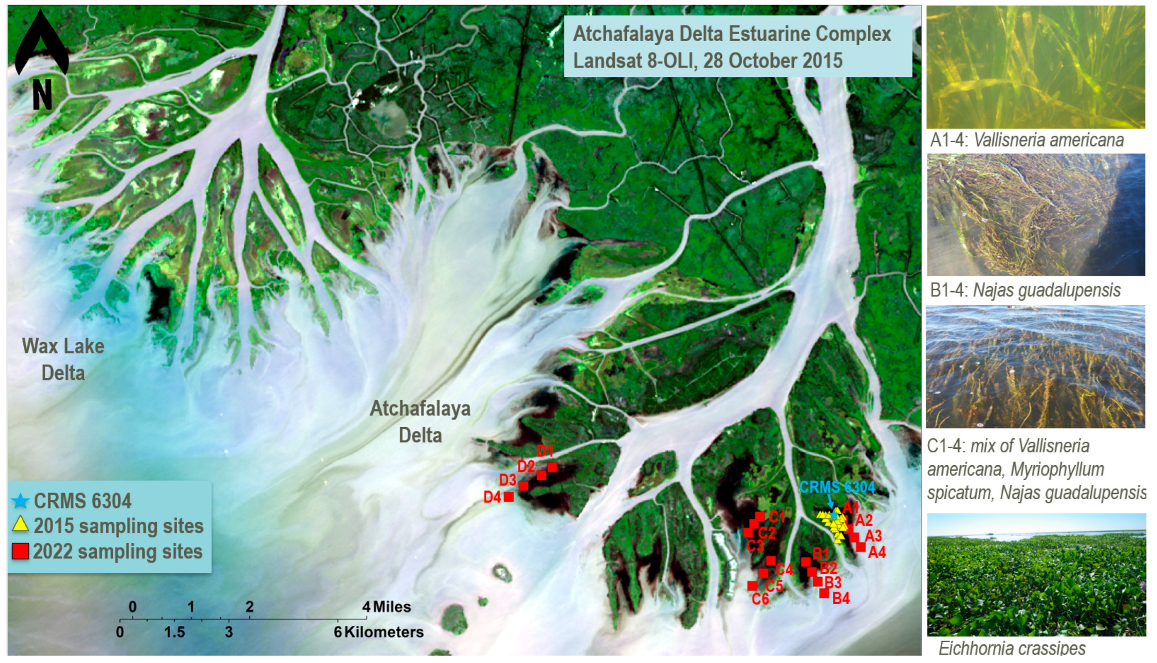
2.1. Study Area

This study focused on approximately 47,000 ha in the southern Atchafalaya Basin, Louisiana, USA (Figure 2). Within the Atchafalaya Basin, two deltas (Atchafalaya Delta and Wax Lake Delta) have formed and are extending southward toward the Gulf of Mexico. These deltas are the result of sediment accretion from the Atchafalaya River discharge and from dredged material deposited by the U.S. Army Corps of Engineers [58,59]. The large volume of fresh, sediment, and nutrient-rich water flowing across the deltas has created an extensive habitat for emergent marsh, floating aquatic vegetation (FAV), and SAV [60]. Intermittently flooded upper deltaic areas are dominated by a diverse assemblage of emergent fresh–intermediate marsh species (e.g., Typha spp., Phragmites australis, and Zizaniopsis miliacea; [61]). Emergent marsh vegetation species tolerant of both continuous and partial submergence, FAV, and SAV, dominate the lower regions of the delta system [60,62]. The abundant SAV and FAV communities of the Atchafalaya River Delta Estuary respond strongly to high turbidity events, especially during periods of seasonal high water [63] as well as major tropical events, such as hurricanes Barry in 2019 and Ida in 2021 [64,65].

2.2. Field Observations

2.2.1. Historical Data

In this study, historical field measurements of SAV and FAV percent cover (% cover) collected by Darnell et al. (unpublished data) between May and September 2015 were used as input to a U-Net model to classify the two habitat types (described in detail in Section 2.3.2). These data were collected at a mean depth of 0.46 m near the mouth of the Atchafalaya River. Thirty sites were sampled adjacent to Coastwide Reference Monitoring System (CRMS) site 6304 (91.2752272°W, 29.4237544°N; Figure 2). Sites were randomly selected using a generalized random tessellation stratified (GRTS) design. SAV % cover from four replicate 0.25 m quadrats was collected during the monthly sampling at each of the 30 sites from May to September 2015. Data summarized from the CRMS stations describe the ranges of mean salinity (1–2.5 ppt), mean water temperature (20.15–36.1 °C) and mean water depth (0.22–1.25 m) during the period of May–September 2015. The SAV % cover data were categorized for subsequent analyses: high density (60–100%; SAV high), medium density (30–60%; SAV medium), and low density (0–30%; SAV low) based upon a modified Braun–Blanquet scale [64].

2.2.2. Field Data Collection for U-Net Model Validation

To validate the SAV mapping from remote sensing data using the U-Net model, SAV % cover, presence/absence, and dominant species of SAV were assessed in the Atchafalaya River Delta on 19 October 2022. SAV observations were collected along four transects (A, B, C, and D; Figure 2). Four sampling stations were randomly selected along each transect. Due to the low water levels restricting access, some stations had to be re-located along the transects. At each sampling station, five replicate 0.25 m² quadrats were measured for SAV % cover. The dominant species of SAV, water temperature (°C), mean water depth (m), salinity (ppt), and location (latitude and longitude) were recorded at each sampling station. The mean % cover of each individual SAV species (±standard deviation) was determined by calculating the average across five replicate samples at each station. The total SAV % cover across all species (versus bare sediment) was then calculated as the sum of the mean % cover measurements for all SAV species observed at each station. The total SAV % cover was then classified into low (0–30%), medium (30–60%), and high (60–100%).

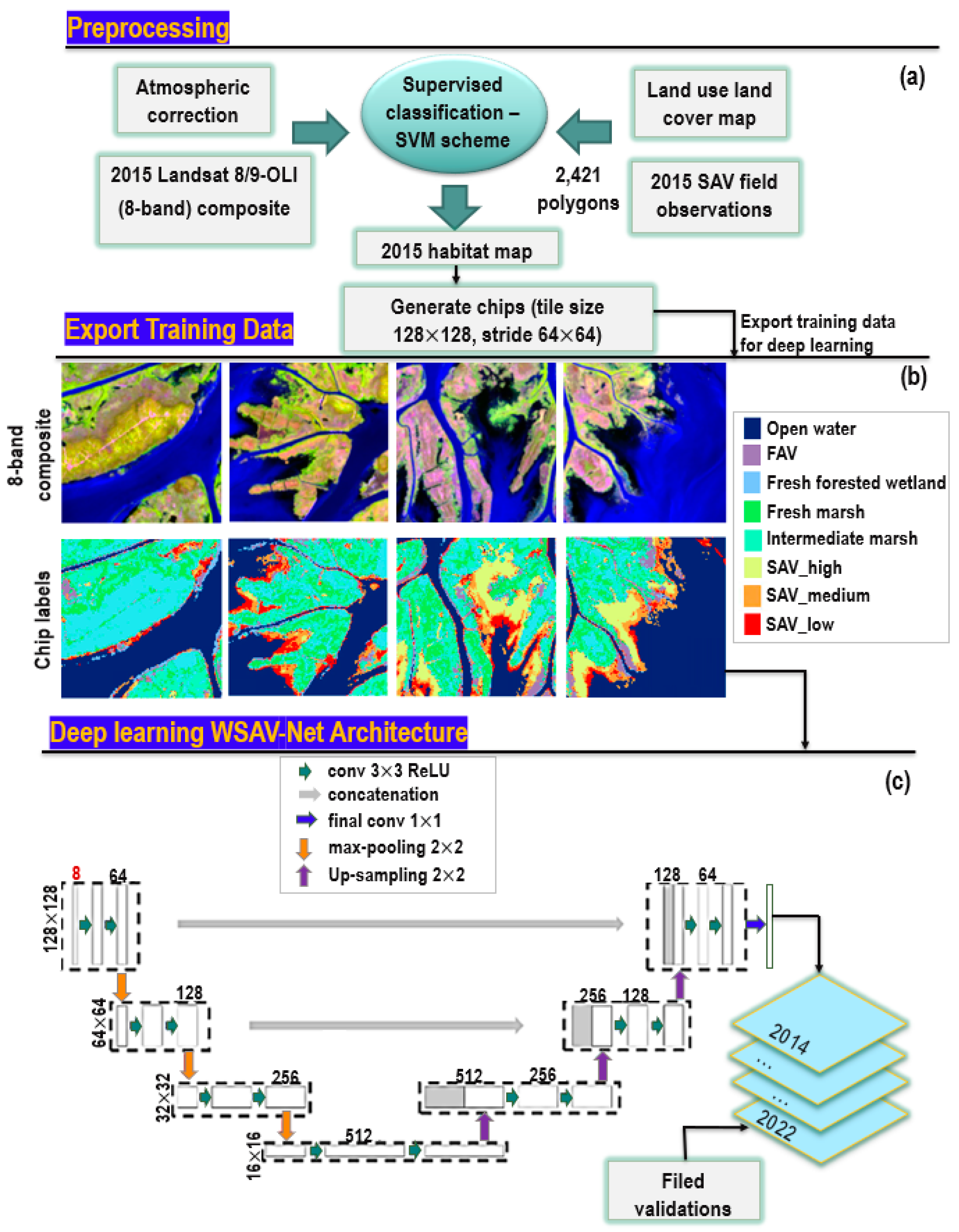
2.3. Deep Learning for Habitat Classification

In this study, a deep learning model based on the U-Net architecture was established to classify the wetland habitat types (fresh forested wetland, fresh marsh, intermediate marsh, brackish marsh, FAV, SAV (high, medium, and low), open water, and bare ground) using Landsat 8/9-OCI. The model developed was named Wetland-SAV Network (hereafter, WSAV-Net).

2.3.1. Remote Sensing Data and Processing

The Operational Land Imager (OLI) sensors onboard Landsat 8 and 9 platforms (Landsat 8/9-OLI) offers innovative opportunities for the long-term observation and monitoring of coastal habitats with a medium spatial resolution at 30 m [66,67]. The orbits of these two satellites are designed to shorten the revisit interval to substantially increase the temporal resolution [68]. In this study, a total of seven Level-1C Landsat 8/9-OLI images (

Table 1. List of satellite data used in this study.

#	Date	Satellite Sensor	File Name
1	28 October 2015	Landsat 8-OLI	LC08_L1TP_023039_20151028_20200908_02_T1
2	30 October 2016	Landsat 8-OLI	LC08_L1TP_023039_20161030_20200905_02_T1
3	17 October 2017	Landsat 8-OLI	LC08_L1TP_023039_20171017_20200902_02_T1
4	23 October 2019	Landsat 8-OLI	LC08_L1TP_023039_20191023_20200825_02_T1
5	26 September 2021	Landsat 8-OLI	LC08_L1TP_023039_20210926_20211001_02_T1
6	21 September 2022	Landsat 9-OLI	LC09_L1TP_023039_20220921_20220923_02_T1
7	15 October 2022	Landsat 8-OLI	LC08_L1TP_023039_20221015_20221021_02_T1

) were downloaded from USGS Earth Explorer (https://earthexplorer.usgs.gov/, accessed on 31 May 2023). Landsat 8-OLI images obtained on 19 September 2015 were within ±3 days of historical field measurements of % cover (Section 2.2.1). The Landsat 8-OLI imagery obtained on 15 October 2022 were within ±5 days of field measurements of SAV % cover collected on 19 October 2022 (Section 2.2.2). Satellite images acquired in September/October were used to capture the peak growing season for SAV, in addition to a period of low cloud cover. The Level 1C images, which are top of atmosphere (TOA) reflectance (${\mathsf{\rho }}_{\mathrm{T}\mathrm{O}\mathrm{A}}$) were processed to obtain bottom of atmosphere (BOA) Level-2A surface reflectance (${\mathsf{\rho }}_{\mathrm{s}}$). ENVI’s FLAASH (Fast Line-of-sight Atmospheric Analysis of Hypercubes) atmospheric correction tool was used to complete the radiation calibration and atmospheric correction. Surface reflectance at six original bands, including blue, green, red, near-infrared (NIR), shortwave infrared 1 (SWIR1) and 2 (SWIR2) together with the normalization difference vegetation index (NDVI [69] and the modified normalized difference water index; MNDWI [70] were used to generate a 8-band composite image for WSAV-Net training (Figure 3).

2.3.2. Louisiana Wetland-SAV Network Model (WSAV-Net)

Land use land cover data (LULC) [71] containing 67 vegetation species across coastal Louisiana were grouped into habitat types according to Visser and Duke-Sylvester [72]. These data were then used to label 8-band composite imagery for the image acquired on 19 September 2015. However, the SAV habitat in the LULC map lacked % cover information. Thus, the SAV % cover data obtained in September 2015 were used to identify SAV % cover as low, medium, or high for the imagery acquired on 19 September 2015. As a result, a total of 2421 polygons were characterized as one of 10 habitat types including fresh forested wetland, fresh marsh, intermediate marsh, brackish marsh, FAV, SAV (high, medium, and low), open water, and bare ground. These polygons were used for supervised classification using the support vector machine (SVM) scheme, where the marshes and bare ground referrer to emergent habitats. The 10-category habitat map from the supervised classification in combination with the 8-band composite image acquired on 19 September 2015 was further cropped to image chips at fixed size (128 × 128 pixels) to train WSAV-Net (Figure 3) to identify habitat types (n = 1802 chips).

The encoder–decoder framework of WSAV-Net is a typical U-Net architecture (Figure 3). This was used to extract landscape features and predict vegetation type labels. In WSAV-Net, the encoding path is composed of 3 convolutional blocks including two 3 × 3 convolution layers with a rectified linear unit (ReLU) activation (green arrows; Figure 3) followed by a max-pooling layer with a 2 × 2 pool size. The input 8-band composite chips are down-sampled into a series of feature maps through convolutional blocks. Each block in the decoder path consists of an up-sampling layer, a concatenation with the corresponding block from the encoder path, and two convolutional layers. The last layer of the network is a 1 × 1 convolution (blue arrow; Figure 3) with Sigmoid activation. An initial learning rate of 10⁻⁴ was used. The training batch size was set to eight and the epoch was set to 50, where epoch is defined as the one entire passing of training data through the model. The WSAV-Net employed the Keras library with TensorFlow with its learning processes trained using NVIDIA Tesla T4 GPU.

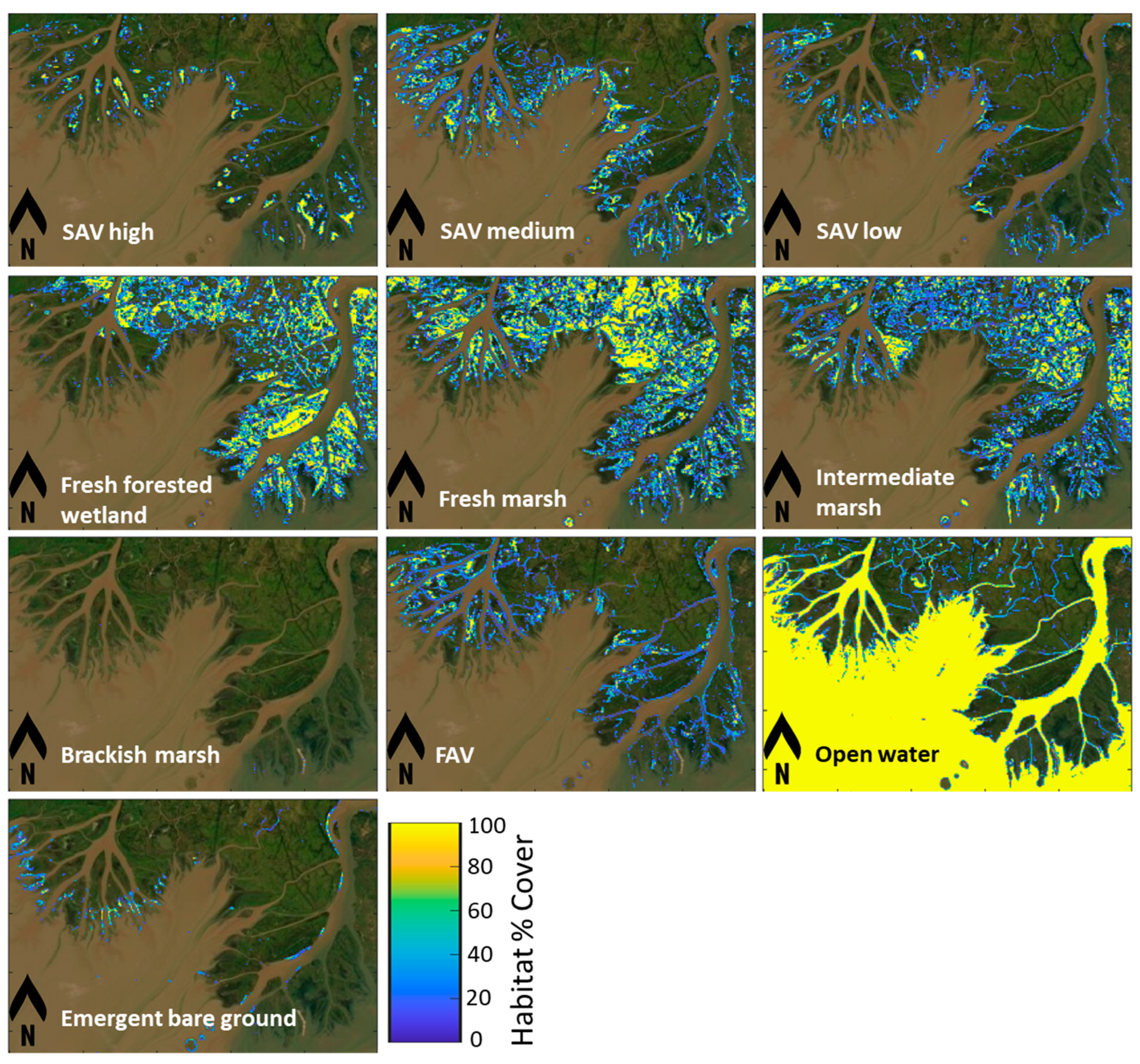
2.3.3. Habitat Percent Cover

To investigate the effect of changes in habitat % cover on the net GHG flux per hectare (i.e., 100 m × 100 m), habitat maps with 30 m resolution produced from WSAV-Net were converted into habitat % cover using 90 m resolution grids as shown in Equation (1).

$${\mathrm{H}\mathrm{a}\mathrm{b}\mathrm{i}\mathrm{t}\mathrm{a}\mathrm{t} \% \mathrm{c}\mathrm{o}\mathrm{v}\mathrm{e}\mathrm{r}}_{\mathrm{i}}=\frac{\sum {\mathrm{N}\mathrm{u}\mathrm{m}\mathrm{b}\mathrm{e}\mathrm{r} \mathrm{o}\mathrm{f} \mathrm{h}\mathrm{a}\mathrm{b}\mathrm{i}\mathrm{t}\mathrm{a}\mathrm{t} \mathrm{p}\mathrm{i}\mathrm{x}\mathrm{e}\mathrm{l}}_{\mathrm{i}}\times 30 \mathrm{m} \times 30 \mathrm{m}}{\mathrm{A}\mathrm{r}\mathrm{e}\mathrm{a} \mathrm{o}\mathrm{f} \mathrm{a} 90 \mathrm{m} \times 90 \mathrm{m} \mathrm{g}\mathrm{r}\mathrm{i}\mathrm{d} \mathrm{c}\mathrm{e}\mathrm{l}\mathrm{l}}$$

(1)

where ${\mathrm{H}\mathrm{a}\mathrm{b}\mathrm{i}\mathrm{t}\mathrm{a}\mathrm{t} \% \mathrm{c}\mathrm{o}\mathrm{v}\mathrm{e}\mathrm{r}}_{\mathrm{i}}$ refers to the percentage of coverage for the i-th habitat type, and i represents one of 10 habitat types contained in each 90 m grid cell (i.e., fresh forested wetland, fresh marsh, intermediate marsh, brackish marsh, FAV, SAV in high, medium, and low, open water, and bare ground). The sum of all percentages of habitat types in each grid cell equals 100%.

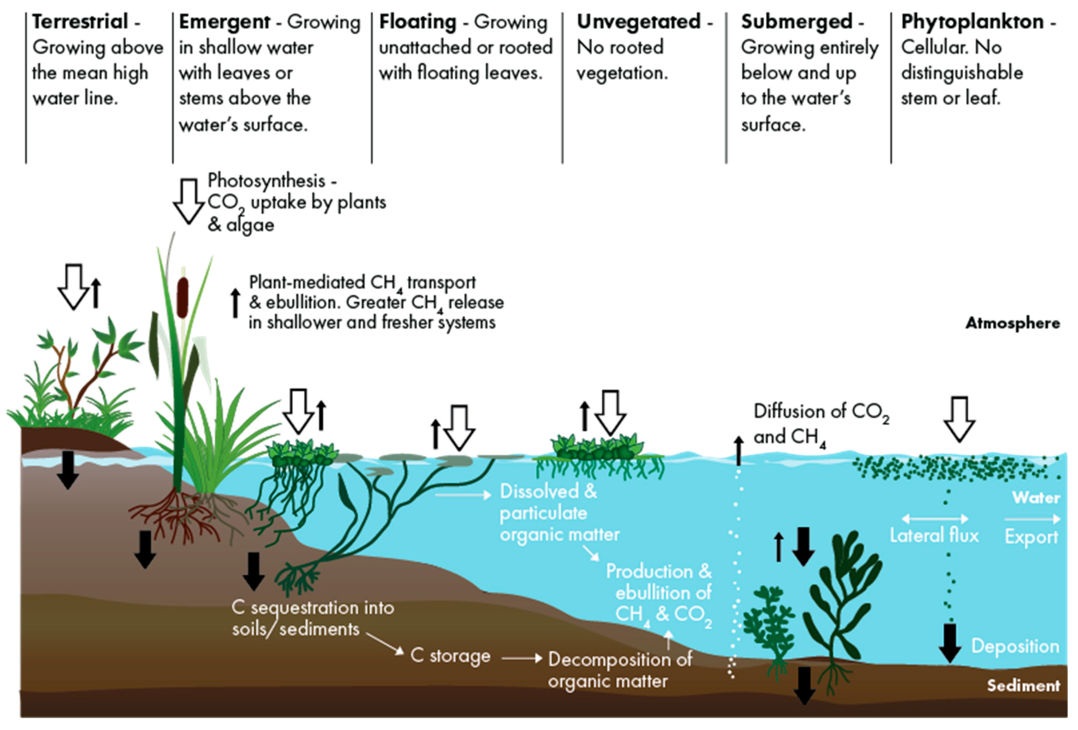
2.4. Carbon Balance Model

To quantify the carbon captured and stored in coastal habitats, a Net Ecosystem Carbon Balance approach was used (NECB; [73]). This methodology is based on carbon fluxes (e.g., g C m⁻² y⁻¹) and is frequently used in ecological studies to assess the net carbon balance (gain or loss) of coastal habitats [74,75,76,77,78]. Carbon fluxes of the aboveground net primary productivity (ANPP), sediment/soil accumulation rates (Sed./Soil_accum.), as well as methane (CH₄) and nitrous oxide (N₂O) emissions are commonly included in the coastal habitat assessments that inform GHG inventories [79,80,81].

To assess the NECB of non-marine SAV habitats in Louisiana’s fresh and intermediate environments, peer-reviewed literature, and scientific data were reviewed to obtain ANPP, soil carbon accumulation rate, and CH₄ emissions; note that N₂O was not considered in the NECB calculation for SAV habitats due to limited data availability. Subsequently, CH₄ emissions were converted into their carbon dioxide equivalent (CO₂e) by multiplying by a global warming potential (GWP) index value of 25 [81,82,83,84]. The mean value of all the observational means (“global mean”) extracted from peer-reviewed literature and scientific data was used to create an SAV carbon flux look-up table. All units in the look-up table were converted into tonnes CO₂e ha⁻¹ y⁻¹ with a standard error of the mean (SE). For other wetland habitats, the overall mean carbon fluxes were obtained from Baustian et al. [85,86] (Supplementary Table S2).

The modified NECB is calculated based on habitat-specific carbon fluxes, as shown in Equation (2).

$${\mathrm{N}\mathrm{E}\mathrm{C}\mathrm{B}}_{\mathrm{i}}={\mathrm{A}\mathrm{N}\mathrm{P}\mathrm{P}}_{\mathrm{i}}+{\mathrm{S}\mathrm{e}\mathrm{d}./\mathrm{S}\mathrm{o}\mathrm{i}\mathrm{l}}_{\mathrm{a}\mathrm{c}\mathrm{c}\mathrm{u}\mathrm{m}. \mathrm{i}}+{\mathrm{G}\mathrm{H}\mathrm{G}}_{\mathrm{i}}$$

(2)

where i represents 1 of 10 habitats considered in this study (i.e., fresh forested wetland, fresh marsh, intermediate marsh, brackish marsh, FAV, SAV, (high, medium, and low), and open water).

• ANPP = aboveground net primary productivity which represents the live AG biomass produced within one year (tonne CO₂e ha⁻¹ y⁻¹).
• Sed./Soil_accum. = net carbon accumulation in sediment for SAV and open water or in soils for wetlands (tonne CO₂e ha⁻¹ y⁻¹). Incorporates the live or net primary productivity of belowground biomass, the accumulation of dead belowground biomass of roots and rhizomes, aboveground litter, and allochthonous carbon [77].
• GHG = GHG emissions (tonne CO₂e ha⁻¹ y⁻¹) including CH₄ and N₂O. CO₂ is excluded because ANPP and Sed./Soil_accum. represent the net value of CO₂ balance.

The net GHG flux of emissions (tonne CO₂e) at each grid cell (90 m) was further determined by the product of the NECB for each habitat and its corresponding habitat area [74], as shown in Equation (3).

$$\mathrm{N}\mathrm{e}\mathrm{t} \mathrm{G}\mathrm{H}\mathrm{G} {\mathrm{f}\mathrm{l}\mathrm{u}\mathrm{x}}_{\mathrm{g}\mathrm{r}\mathrm{i}\mathrm{d} \mathrm{c}\mathrm{e}\mathrm{l}\mathrm{l}}={\sum }_{\mathrm{i}=1 \mathrm{t}\mathrm{o} 10}{\mathrm{N}\mathrm{E}\mathrm{C}\mathrm{B}}_{\mathrm{i}}\times {\mathrm{F}}_{\mathrm{i}}\times {\mathrm{A}\mathrm{r}\mathrm{e}\mathrm{a}}_{\mathrm{g}\mathrm{r}\mathrm{i}\mathrm{d} \mathrm{c}\mathrm{e}\mathrm{l}\mathrm{l}}$$

(3)

where i represents one of 10 habitats considered in this study (i.e., fresh forested wetland, fresh marsh, intermediate marsh, brackish marsh, FAV, SAV (high, medium, and low), open water, bare ground). F_i represents % cover of habitat_i. The % cover of SAV in high is set to 100%. The % cover of SAV in medium and low categories were set to 56% and 19%, respectively, using the median values of each classification. A positive value for the net GHG flux indicates a GHG source to the atmosphere and a negative value indicates a net GHG sink from the atmosphere.

2.5. Accuracy Analysis

Four evaluation indices were used to assess the accuracy of the WSAV-Net classification: probability of false detection (${\mathrm{P}}_{\mathrm{f}}$), precision, recall, and F₁ score. The F₁ score is the measure of a model’s accuracy on a dataset, which is a way of combining the precision and recall of the model and is defined as the harmonic mean of the model’s precision and recall [87]. The precision, recall, and F₁ scores were calculated for all classes using a macro-average method (an equal weight per class); for more details, refer to Supplement S1.

Furthermore, uncertainty analyses were conducted for (1) carbon fluxes (ANPP, Sed./Soil_accum., and GHG emissions) per habitat; (2) NECB estimations per habitat; and (3) net flux of GHG emissions for the study area based on U.S. Environmental Protection Agency (EPA) method [81]. The percentage of uncertainty (% uncertainty) in the carbon fluxes was calculated based on the standard error (SE) and the mean of carbon flux as seen in Equation (4).

$$\mathrm{P}\mathrm{e}\mathrm{r}\mathrm{c}\mathrm{e}\mathrm{n}\mathrm{t}\mathrm{a}\mathrm{g}\mathrm{e} \mathrm{u}\mathrm{n}\mathrm{c}\mathrm{e}\mathrm{r}\mathrm{t}\mathrm{a}\mathrm{i}\mathrm{n}\mathrm{t}\mathrm{y} = \left(\frac{{\mathrm{c}\mathrm{a}\mathrm{r}\mathrm{b}\mathrm{o}\mathrm{n} \mathrm{f}\mathrm{l}\mathrm{u}\mathrm{x}}_{\mathrm{S}\mathrm{E}}}{{\mathrm{c}\mathrm{a}\mathrm{r}\mathrm{b}\mathrm{o}\mathrm{n} \mathrm{f}\mathrm{l}\mathrm{u}\mathrm{x}}_{\mathrm{m}\mathrm{e}\mathrm{a}\mathrm{n}}}\right)\times 100\%$$

(4)

The combined uncertainty was further calculated for NECB using the simple error propagation method, see Equation (5) [88,89,90]:

$$\mathrm{C}\mathrm{o}\mathrm{m}\mathrm{b}\mathrm{i}\mathrm{n}\mathrm{e}\mathrm{d} \mathrm{u}\mathrm{n}\mathrm{c}\mathrm{e}\mathrm{r}\mathrm{t}\mathrm{a}\mathrm{i}\mathrm{n}\mathrm{t}\mathrm{y} = \sqrt{{\left({\mathrm{A}\mathrm{N}\mathrm{P}\mathrm{P}}_{\% \mathrm{u}\mathrm{n}\mathrm{c}\mathrm{e}\mathrm{r}\mathrm{t}\mathrm{a}\mathrm{i}\mathrm{n}\mathrm{t}\mathrm{y}}\right)}^2+{\left({\mathrm{S}\mathrm{e}\mathrm{d}./\mathrm{S}\mathrm{o}\mathrm{i}\mathrm{l} \mathrm{a}\mathrm{c}\mathrm{c}\mathrm{u}\mathrm{m}.}_{\% \mathrm{u}\mathrm{n}\mathrm{c}\mathrm{e}\mathrm{r}\mathrm{t}\mathrm{a}\mathrm{i}\mathrm{n}\mathrm{t}\mathrm{y}}\right)}^2+{\left({\mathrm{G}\mathrm{H}\mathrm{G} \mathrm{e}\mathrm{m}\mathrm{i}\mathrm{s}\mathrm{s}\mathrm{i}\mathrm{o}\mathrm{n}\mathrm{s}}_{\% \mathrm{u}\mathrm{n}\mathrm{c}\mathrm{e}\mathrm{r}\mathrm{t}\mathrm{a}\mathrm{i}\mathrm{n}\mathrm{t}\mathrm{y}}\right)}^2}$$

(5)

3. Results

3.1. Field Observations of SAV Percent Cover

Overall, the SAV communities observed in transects A–D in 2022 were primarily dominated by Vallisneria americana and Najas guadalupensis (

Table 2. Field observation of SAV % cover (% of quadrat covered with SAV vs. bare sediment) obtained from the Atchafalaya River Delta in October 2022; assigned categories of SAV cover were 0–30% (low), 30–60% (medium), and 60–100% (high).

Total SAV % Cover from Field	SAV % Cover Categorized from Field Measurements	SAV % Cover Classified from Remote Sensing	Dominant Species	% Cover of Dominant Species	Sampling Stations
61%	High	SAV medium	V. americana	46%	A3
64%	High	SAV medium	V. americana	63%	C4
64%	High	SAV medium	V. americana	64%	D3
72%	High	SAV high	V. americana	72%	C2
73%	High	SAV high	N. guadalupensis	67%	B3
75%	High	SAV high	V. americana	73%	A2
79%	High	SAV high	V. americana	73%	A1
85%	High	SAV high	V. americana	85%	B2
86%	High	SAV high	N. guadalupensis	63%	B1
95%	High	SAV high	V. americana	93%	D2
35%	Medium	SAV low	N. guadalupensis	19%	B4
44%	Medium	SAV medium	V. americana	44%	C5
51%	Medium	SAV medium	V. americana	51%	C1
16%	Low	SAV low	N. guadalupensis	15%	C6
22%	Low	SAV low	N. guadalupensis	18%	D4
23%	Low	SAV low	N. guadalupensis	11%	C3
27%	Low	SAV low	V. americana	27%	A4

Total % cover of SAV observed from field observations were further compared with WSAV-Net output of SAV % cover (Section 3.3.1).

). The dominant species observed at each station and their % cover are provided in Table 2 (columns 4 and 5, respectively). The measured SAV % cover ranged from 61% (transect A, site 3) to 95% (transect D, site 2) in the high category, 35% (transect B, site 4) to 44% (transect C, site 5) in the medium category, and 16% (transect C, site 6) to 27% (transect A, site 4) in the low category (Table 2). It was observed that the SAV habitat characterized as low % cover was primarily composed of N. guadalupensis, whereas medium and high % cover areas were dominated by V. americana. For example, V. americana was the primary species observed in transect A, and mean SAV % cover was observed to decrease along the transect (A1–4), with the highest SAV % cover observed at the station closest to the emergent marsh (A1: 79%), decreasing with greater distance from the marsh (A4: 27%). Species composition along transect B was primarily V. americana and N. guadalupensis, with three of the four sites classified as high SAV % cover. Sampling sites C1–6 were divided into two transects with three sampling sites in each (Figure 2). V. americana and N. guadalupensis were also the dominant SAV species present in transects C and D; as in transect A, the % cover decreased with increasing distance from the emergent marsh.

3.2. Carbon Flux Look-Up Table

Carbon flux data were limited for fresh and intermediate salinity SAV habitats in Louisiana (

Table 3. Major carbon fluxes (ANPP, sediment accumulation rate, and GHG emissions) for fresh and intermediate salinity SAV habitats extracted from the literature. Carbon flux values that could not be sourced from the literature are represented by N/A.

Area of Interest (Location)	Salinity (ppt)	Carbon Fluxes (Tonne CO2e ha−1 y−1)
		ANPP	Sed.accum.	GHG fluxes	Citation
Wuliangsu Lake, China	Fresh	N/A	N/A	4.73	[91]
Luanhaizi wetland, China	Fresh	N/A	N/A	2.84	[92]
Lake Taihu, China	Fresh	N/A	N/A	2.04	[93]
Everglades Stormwater Treatment Areas, FL	0–10	N/A	−17.8	N/A	[94]
Indoor mesocosm of Myriophyllum spicatum	Fresh	N/A	−5.60	N/A	[95]
Mississippi River Delta Plain, LA	0–0.2	−2.34	N/A	N/A	[20]
Mississippi River Delta Plain, LA	0.2–7.2	−2.50	N/A	N/A	[20]
Fresh and intermediate marsh SAV, LA	0.5–5	−2.50	N/A	N/A	[96]
Gulf coast sites	0–0.5	−1.32	N/A	N/A	[19]
Atchafalaya delta, LA	0.5–5	−0.27	N/A	N/A	[1]
Birds foot delta, LA	0.5–5	−1.70	N/A	N/A	[97]
Chenier Plain, LA	0.5–6.5	−0.34	N/A	N/A	[98]
Barataria bay, LA	0.5–5	−0.47	N/A	N/A	[99]
Rockefeller State Wildlife Refuge, LA	0–6	−0.78	N/A	N/A	[100]
Overall mean ± SE	-	−1.40 ± 0.31	−11.7 ± 6.1	3.20 ± 0.79	-

); thus, the Sed._accum. and GHG emissions from SAV habitat were obtained from studies conducted outside of Louisiana whose primary focus was the same fresh/intermediate SAV species as that reported in Louisiana. The mean ANPP from the literature ranged from −0.27 to −2.50 tonne CO₂e ha⁻¹ y⁻¹ and the overall mean (±SE) was −1.40 (±0.31) tonne CO₂e ha⁻¹ y⁻¹ (Table 3). From these studies, the overall mean Sed._accum. was −11.7 ± 6.1 tonne CO₂e ha⁻¹ y⁻¹. SAV habitats were observed to sequester more carbon compared to open water habitats (−8.6 ± 6.3 tonne CO₂e ha⁻¹ y⁻¹; Supplement S2). GHG gas flux estimates for this study were based on the values of CH₄ emissions observed in fresh–intermediate salinity SAV habitats. The mean GHG flux was 3.20 ± 0.79 tonne CO₂e ha⁻¹ y⁻¹. Given the limited availability of N₂O measurements, mean GHG fluxes relied exclusively on CH₄ flux measurements obtained from literature sources. These measurements were derived using distinct methodologies, encompassing static chamber measurements [91,92] and the application of the eddy covariance system [93] (Table 3). Such methodological differences may introduce uncertainties in CH₄ flux assessment for SAV habitats.

The SAV habitat area contained a mix of open water and SAV species; as such, ANPP for both open water and SAV habitats were included in the NECB for SAV habitats. Open-water ANPP for the whole cell was added to SAV ANPP, pro-rated by the mean % cover of SAV. ANPP from the open water habitat was added to SAV ANPP to account for the phytoplankton production in the water column above benthic SAV communities. Therefore, the total NECB of SAV habitats (SAV plus overlying water column) in the study area was −13.6 ± 7.9 tonne CO₂e ha⁻¹ y⁻¹ (Supplement S2). In addition, the fresh forested wetland (NECB = −0.7 ± 0.4 tonne CO₂e ha⁻¹ y⁻¹) served as another GHG sink within the study area (Supplement S2). There were limited available literature values for ANPP, Sed._accum., and GHG emissions for FAV habitats; therefore, FAV was combined into a fresh marsh for further analysis. Lastly, all other habitats in the study area were considered as GHG sources (including fresh and intermediate marsh) due to the assumed higher CH₄ emission in fresh and intermediate marsh environments [101,102]. The emergent bare ground in the study area was not modeled in this analysis and thus was assumed to have net zero carbon fluxes for all calculations.

3.3. Remote Sensing of Habitats

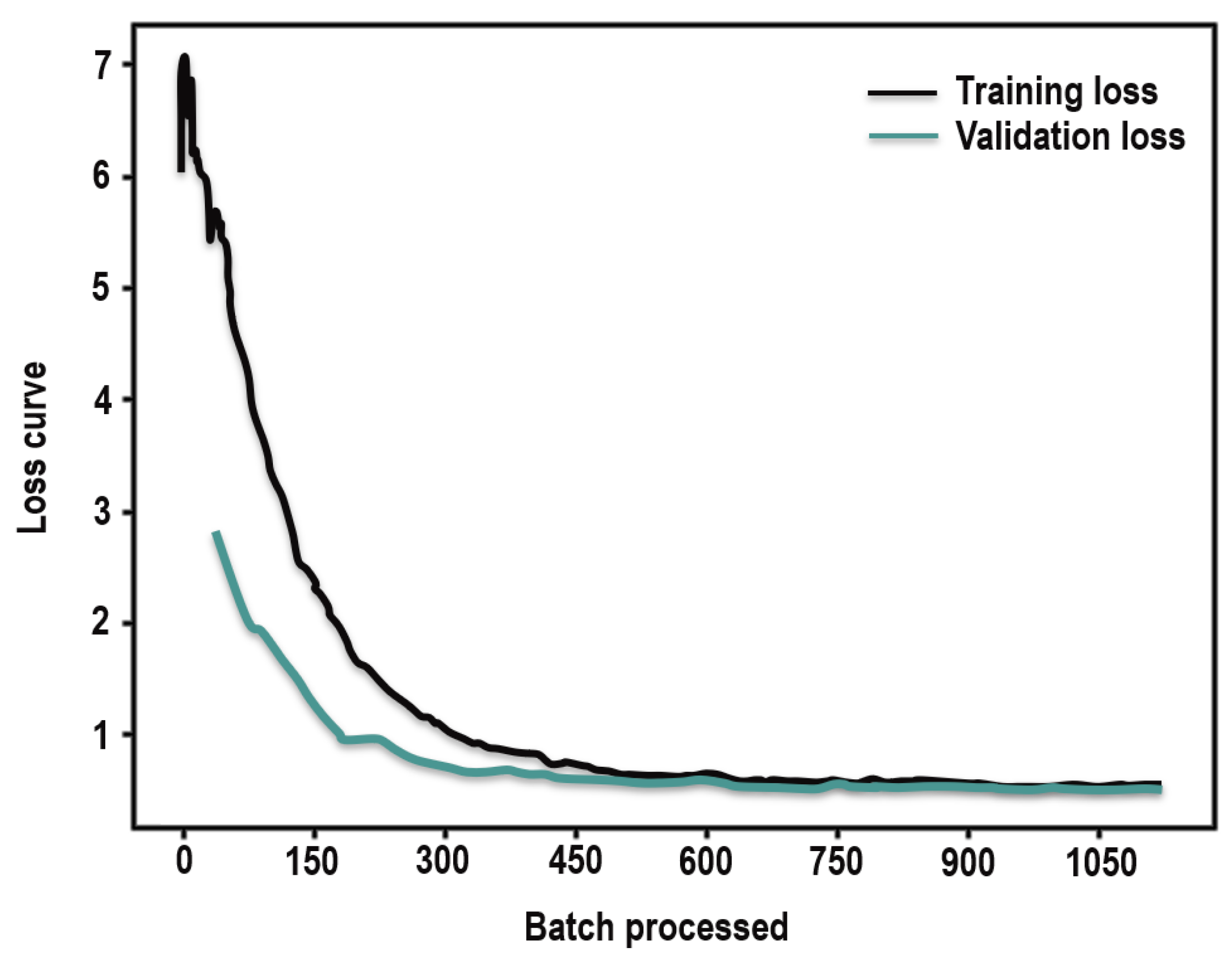
3.3.1. Deep Learning Model Performance

The accuracy of the trained WSAV-Net was 83.7% with F₁ scores ranging from 58.2 to 98.4% (

Table 4. The metrics of WSAV-Net, including precision, recall, and F₁ score, for coastal habitat classification from remote sensing imagery.

Metrics Habitats	Precision (%)	Recall (%)	F1 Score (%)	Overall Accuracy (%)
Fresh forested wetland	81.2	71.9	76.4	86.7%
Fresh marsh	86.4	73.2	79.8
Intermediate marsh	74.3	83.1	78.7
Brackish marsh	52.3	64.2	58.2
FAV	79.1	79.5	79.2
SAV high	80.5	77.4	78.9
SAV medium	69.3	71.9	70.6
SAV low	78.5 69.3	79.2	78.9
Open water	97.3	99.6	98.4

), indicating an overall good performance of WSAV-Net when classifying habitats from remote sensing imagery [103,104]. The lowest F₁ score was observed for brackish marsh due to limited training and validation data. Furthermore, the loss function (or learning curve) of a well-performing U-Net model is expected to show a decreasing asymptotic curve over time [105]. This was the case for the learning curve of WSAV-Net, showing a high training and validation loss at the beginning which decreased to a point of stability with increasing training samples (Figure 4). The gap between the validation and training loss shrinks after each epoch, with a minor difference between the validation and training loss. This illustrates the typical feathers of the learning curve of a good model [106]. In addition, the learning curve is also known to be an efficient approach by which to identify overfitting and underfitting problems [105]. In this study, based on the learning curve, no under- or over-fitting issues were detected. A model which is overfitting will learn training data perfectly with the result that the model misclassifies unseen data. Thus, the learning curve of an overfitting model has a low training loss at the beginning, which gradually increases with slightly increasing training data and does not reach an asymptote [106]. In addition, the training and validation losses of an overfitting model are far away from each other, which also was not seen in the learning curve from this study. In contrast, the learning curve of an underfitting model, which is unable to recognize meaningful patterns in the data, could be flat or noisy regardless of the amount of training data. Additionally, a gradual increase in training loss at the beginning and sudden dip in both training and validation losses at the end without approaching an asymptote can indicate a model that is underfitting [105].

Field observations of SAV % cover collected in 2022 demonstrated that the WSAV-Net could successfully identify both a high and low % cover of SAV (Table 2). There were some differences, namely that WSAV-Net classified the SAV with up to 65% cover as a break point for the SAV medium, which was higher than the manually classified 60%. For example, there were nine sampling sites with SAV % cover in the range of 60–100%. Only six of these were classified as SAV high by WSAV-Net, and the remainder were classified as SAV medium (A3: 61%, C4: 62.6%, and D4: 64%). In comparison, for low-abundance SAV sites, with an SAV % cover of less than 30%, WSAV-Net correctly classified them all as SAV low. Therefore, based on the classification from WSAV-Net, % cover in the range of 0–30% was effective for detection as the SAV low. However, the SAV medium and high were more likely to be detected using the ranges of 30%–65% and >65%, respectively.

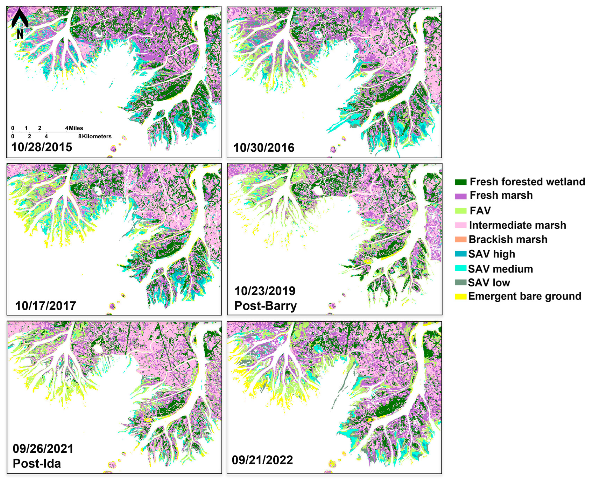
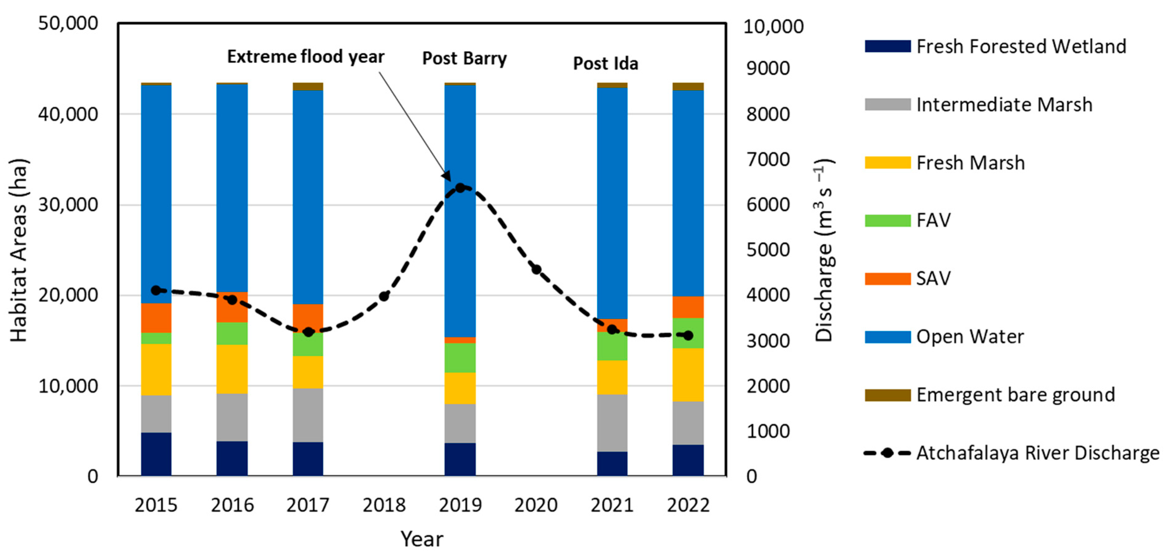
3.3.2. Habitat Changes from 2015 to 2022

Habitat maps that characterized eight habitat types were developed for the years 2015, 2016, 2017, 2019, 2021, and 2022 (Table 1, Figure 5). Overall, approximately half of the study area was dominated by fresh or intermediate marsh habitats for the years quantified, and the remaining area was open water. The spatial coverage of fresh forested wetlands stayed relatively constant during the study period. The area of SAV habitat was relatively stable between 2015 and 2017, with a minor decline from 3465 ha (2015) to 3123 ha (2017). Most of the areas classified as SAV showed medium-to-high density during the years 2015–2017. The SAV habitat area was observed to decrease from 3125 to 688 ha in 2019, of which 556 ha was classified as medium SAV % (30–65%) cover while the open water habitat areas sharply increased (Figure 6). Although the exact reason for the decline in SAV during the peak growing season of July–October 2019 has not been confirmed yet, it is essential to consider external environmental factors that could potentially contribute to this reduction. Notably, the year 2019 experienced extreme flooding conditions, characterized by record-breaking discharges from both the Mississippi River and Atchafalaya River [107]. The unprecedented flooding during this period led to increased turbidity and sedimentation, which reduced the light penetration to SAV and likely hindered the photosynthetic processes crucial for the growth and survival of SAV [2]. In addition, Hurricane Barry made a landfall as a Category 1 hurricane on Marsh Island, Louisiana, with a maximum reported storm-total rainfall of 580 mm near Ragley, Louisiana [108]. The two deltaic islands are approximately 70 km to the east of Hurricane Barry’s track and were exposed to the highest measured storm surge from that storm (~1.86 m near Eugene Island, Louisiana). Barry’s heavy rains elevated river flow rates (9601 m³ s⁻¹) during a flood year (2019) compared to pre-hurricane conditions (8438 m³ s⁻¹) and caused flooding along the banks of the Atchafalaya River near Morgan City, Louisiana (Figure 6). Hurricanes may have inflicted physical damage onto SAV through wave action, and strong currents, uprooting or burying SAV plants and disrupting their growth [109]. The recovery of SAV was not observed until April 2020. However, identifying the exact SAV recovery time following Hurricane Barry and the 2019 flooding event proved to be challenging due to the unavailability of clear imagery during the peak growing season (September–October) of 2020. The lack of suitable imagery during this critical period hindered our ability to precisely assess the timing and extent of SAV recovery following the extreme weather events in 2019. In addition, major hurricanes in 2020 (Supplement S3), such as Hurricane Laura (Category 4) and Hurricane Zeta (Category 2), may have impacted SAV habitats in the Atchafalaya River Delta Estuary. In 2021, another major hurricane (Hurricane Ida; Category 4) made landfall on 29 August 2021 near Port Fourchon [110]. The highest water levels surrounding the two river deltas during that storm were measured at Eugene Island in Atchafalaya Bay (0.5 m MHHW (mean higher high water); Supplement S3; [110]). The SAV habitat area observed in 2021 (post-Ida) was nearly 1449 ha, which was still less than the pre-hurricane levels (2015–2017). In 2022, the Atchafalaya River experienced the lowest discharge (3125 m³ s⁻¹) measured during the study period. The aerial extent of SAV recovered to the pre-2019 (Hurricane Barry) conditions of approximately 3284 ha. Throughout this area, more than two-thirds of the SAV was medium % cover. The newly deposited sediment (bare ground) was primarily observed near the head of Wax Lake Delta, prograding into the adjacent freshwater zone. An increase in FAV was observed along the edges of the deltaic islands as well as within the inundated areas of both deltas post Hurricane Barry. Details of each habitat can be found in Supplement S3.

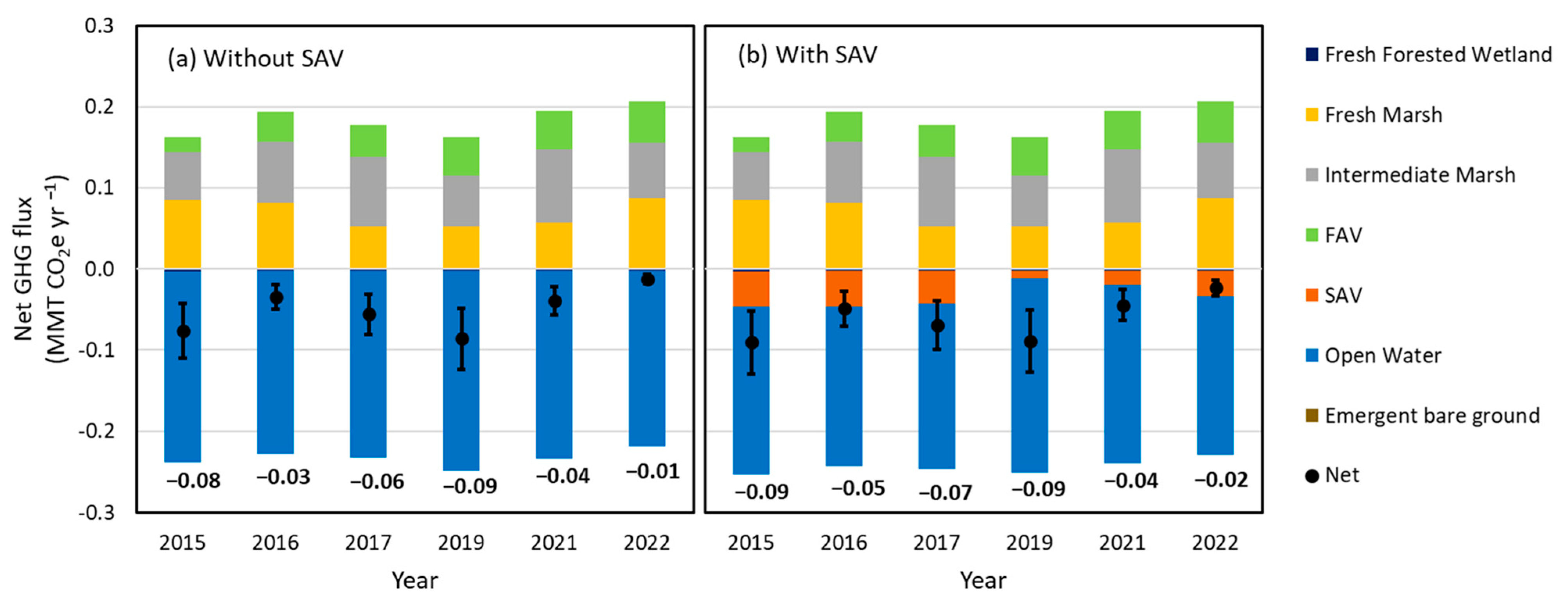
3.4. The Effect of SAV on Net GHG Flux

The carbon fluxes (Section 3.2) and habitat area (Section 3.3) were used to estimate the net GHG fluxes of the study area using a carbon balance model. The calculations of net GHG flux were conducted under two scenarios: a with SAV scenario and a without SAV scenario for the years 2015, 2016, 2017, 2019, 2021, and 2022. In the carbon balance model, habitat maps with 30 m resolution were first converted into habitat % cover using 90 m grids (i.e., 0.81 ha) for the target years. The SAV with different % covers (e.g., SAV high, SAV medium, and SAV low) were considered separately with a different ANPP in carbon calculations by multiplying SAV % cover to the SAV ANPP, estimated from the literature values (Table 3). For the carbon fluxes of SAV habitats from Sed._accum. and GHG, the same carbon fluxes were used regardless of the SAV % cover, as the effect of SAV % cover on Sed._accum. and GHG emissions could not be quantified based upon the available data extracted from the published literature. An example of habitat % cover for ten habitats generated for the year 2015 is shown in (Figure 7). It was noted that FAV was observed to be more widely distributed in the Wax Lake Delta relative to the Atchafalaya Delta. SAV dominated the area along the margins of wetlands. Emergent bare ground was more aggregated adjacent to the head of Wax Lake Delta, transgressing to open water area. The habitat % cover for other target years can be found in Supplementary Figure S3.

3.4.1. Net GHG Fluxes

Net GHG fluxes were estimated as a product of the habitat % cover and NECB for the ten habitats. For the without SAV scenario, carbon fluxes for the open water (e.g., ANPP, Sed._accum., and GHG values) were assigned to SAV habitats in the carbon balance model. The estimated net GHG flux (without SAV scenario) for the study area presented a larger CO₂ sink in 2019 (−0.09 ± 0.04 MMT CO₂e y⁻¹; Figure 8a) than in 2022 (−0.01 ± 0.01 MMT CO₂e y⁻¹; Figure 8a). The negative and positive values of net GHG fluxes represent net atmospheric carbon sinks and sources, respectively. The increase in net GHG sink from 2016 to 2019 resulted from a reduced area of fresh–intermediate marsh and increased the area of open water habitats. In the study areas, the major net CO₂ sources were fresh marsh and intermediate marsh, while the open water habitat was the dominant CO₂ sink in the without SAV scenario (Supplementary Figure S2).

For the with SAV scenario, the estimated net GHG sinks ranged from −0.02 ± 0.01 to −0.09 ± 0.04 MMT CO₂e y⁻¹ during the study period, resulting in an overall higher CO₂ sink observed relative to the without SAV scenario. The inclusion of SAV in the carbon balance model increased net GHG sinks, with the greatest carbon sinks from SAV habitats observed in year 2016 (−0.04 ± 0.02 MMT CO₂e y⁻¹; Supplement S4), which contributed to an estimated more negative GHG flux (−0.05 ± 0.02 MMT CO₂e y⁻¹) in comparison to without SAV scenario (−0.04 ± 0.02 MMT CO₂e y⁻¹). The smallest difference in estimated net GHG fluxes (3.5% difference) was observed in 2019 between with SAV scenario (−0.089 ± 0.04 MMT CO₂e y⁻¹) and without SAV scenario (−0.086 ± 0.04 MMT CO₂e y⁻¹) due to the significant loss of SAV post-Hurricane Barry (Supplement S4 and Supplement S5). Despite the significant loss of SAV habitat after Hurricane Barry in 2019, the estimated net GHG sinks in both scenarios were higher than other years, which was associated with an increase in open water area (Figure 8) due to extreme flooding (Figure 6). Details of each habitat can be found in Supplement S4. Overall, a significant difference of estimated net GHG fluxes between with SAV and without SAV scenarios among years was observed due to the high Sed._accum. of SAV habitats (−11.7 ± 6.1 tonne CO₂e ha⁻¹ y⁻¹; Supplement S2) combined with the ANPP from phytoplankton in the water above the SAV.

3.4.2. Spatial Distribution of Net GHG Fluxes

Spatial distribution maps of estimated net GHG fluxes without SAV and with SAV scenarios, as well as difference maps, were produced for each target year. Examples of net GHG fluxes (90 m resolution) in 2015 are shown in Figure 9a,b (results of other years in Supplement S5). The difference in the net GHG flux between without SAV and with SAV scenarios demonstrated that the SAV increased the estimated net GHG sink by up to 60% (~−5.0 × 10⁻⁶ MMT CO₂e ha⁻¹ y⁻¹) in the open water habitat (Figure 9c). For both scenarios, areas representing a CO₂ source to the atmosphere were highly dominated by fresh–intermediate marsh. For the without SAV scenario (Figure 9a), the areas estimated to be a CO₂ sink in the range of −5.0 to −9.0 × 10⁻⁶ MMT CO₂e ha⁻¹ y⁻¹) were open water habitats. Under the with SAV scenario estimates (Figure 9b), emergent areas were dominated by fresh–intermediate marsh (net CO₂ sources) and were fringed with net GHG sink SAV habitats (ranging from −10 to −15 × 10⁻⁶ MMT CO₂e ha⁻¹ y⁻¹). The distribution of the net GHG fluxes of SAV in the study area estimated that ~1600 ha of the SAV habitat (i.e., about 50% of total SAV habitats (3225 ha) had a net GHG flux between −14.0 and −11.0 × 10⁻⁶ MMT CO₂e ha⁻¹ y⁻¹ in the study area in 2015 (Figure 9d). Spatial distribution maps of the estimated net GHG fluxes and comparisons between without SAV and with SAV scenarios for other target years are presented in Supplementary Figure S5.

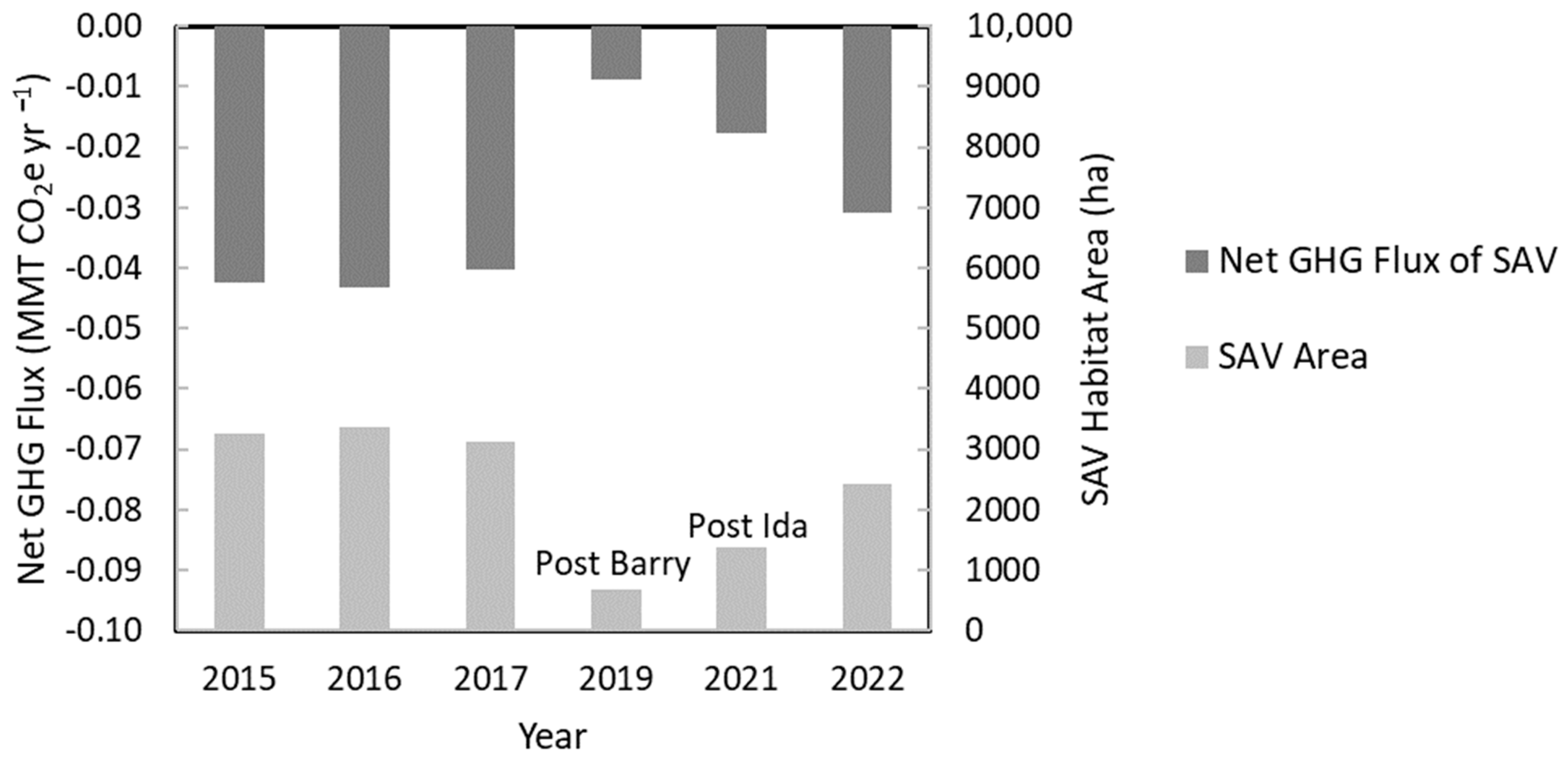
3.4.3. Dynamics of Net GHG Fluxes Pre- and Post-Hurricanes

The effects of hurricanes on net GHG fluxes were investigated by comparing the results from before and after hurricanes Barry and Ida (Figure 10). In 2017, SAV area and net GHG flux were 3125 ha and −0.04 MMT CO₂e y⁻¹, respectively. In comparison, a dramatic decrease in the net GHG flux within the SAV habitat area was observed in 2019 due to a reduction in SAV habitat in the study area (Figure 6). The SAV habitat area was reduced to 688 ha (22% of 2017 SAV area) in the months following Hurricane Barry and extreme flooding event in 2019. As such, the estimated net GHG flux of SAV also reduced to −0.01 MMT CO₂e y⁻¹ in September 2019. In the years post-hurricane, the SAV habitat expanded and was approaching pre-hurricane extent by 2022 (Figure 10). In 2022, during hurricane season, no major storms occurred. During that year (one year after Hurricane Ida and three years after Hurricane Barry), the SAV habitat increased in area with an estimated contribution to net GHG flux equivalent to 77% of the 2017 net GHG flux.

4. Discussion

4.1. SAV Habitat Dynamics and Carbon Fluxes

SAV communities are sensitive to short-term changes in environmental conditions [96,111]. The spatial distribution and abundance of SAV in the study area was more dynamic than in other coastal habitat types due to the area’s hydrodynamics (e.g., water level) and water quality (e.g., turbidity and salinity; [19]). Two major hurricanes occurred during the study period prior to significant temporary decreases in the SAV spatial extent and density throughout the study area. Major storm events and their associated storm surge can increase salinity, turbidity, and wave energy in shallow coastal habitats [112,113]. These major shifts in abiotic conditions have the potential to negatively affect SAV and its associated biota. Frazer et al. [114] observed the increased mortality in both V. americana and M. spicatum after seven days of exposure to increased salinity. Similarly, the SAV recovery in the study area post-hurricane was slow due to continued high water and turbid conditions (from increased river flow), and additional storms (2019–2021 hurricane seasons). However, the SAV rebounded in a single growing season when no major storms or hurricanes occurred (2022 hurricane season). As the impact of hurricanes on SAV habitats can vary depending on various factors such as the intensity and duration of the storm, the location of landfall, and the pre-existing condition of the habitat, methods such as remote sensing can be used to regularly monitor the impact of such events on SAV habitats. High-resolution satellite imagery, such as Sentinel 2-MSI, can also provide detailed information on the seasonal dynamics of SAV, enhancing the temporal observations of SAV habitats. This increased temporal resolution aids in understanding how SAV habitats respond to extreme events and assessing the SAV recovery time. This valuable information could be used to better understand the variability and resilience of SAV meadows, informing management and restoration planning.

Due to the reported high spatial and temporal variation in SAV cover in this region [17,19], the estimation of the net GHG flux for this study was based on existing habitats in the target years in the carbon balance model, rather than on continuous estimates over time (accounting for habitat conversions). Studies of emergent coastal wetlands have estimated carbon loss as emergent wetland converts into open water, ranging from 20% to 100% of soil carbon [115,116,117]. However, similar estimates related to carbon loss in SAV have not been documented, particularly for fresh- and intermediate-salinity SAV species. Thus, the fate of carbon from lost SAV meadows is highly uncertain and requires further empirical field measurements to reduce uncertainty in the annual estimates of SAV net GHG flux. In coastal Louisiana, projections of emergent wetland loss and the associated potential increase in SAV in shallow open water habitats makes investigating carbon capture and sequestration in the sediments of these open water areas increasingly important to reduce uncertainty in the estimates of coastal habitat net GHG fluxes.

4.2. SAV Contributions to Net GHG Flux

To evaluate the potential contribution of SAV to net GHG flux, 43,460 ha of the Atchafalaya River Delta Estuary was selected to estimate GHG emissions under two scenarios—without SAV and with SAV—in the target years (i.e., 2015, 2016, 2017, 2019, 2021, and 2022). For both scenarios, open-water habitats dominated the net GHG sinks and accounted for 57% of the study area. Accounting for SAV in open-water areas increased the total net GHG sinks by up to 40% in the study area. Based on available literature, SAV has a high Sed._accum. and slightly higher NECB than open-water habitats [18,118,119]. However, for the entire 43,460 ha study area, the total net GHG sinks from SAV were lower than for open water due to their much smaller spatial extent (i.e., SAV covered ~12% of the area of the open water). When considered at a hectare scale, open-water areas dominated by SAV increased the net GHG sink by about 60% in comparison with open water without SAV (Figure 9c). It was also observed that the presence of SAV could switch the net GHG flux from source to sink, depending on the fractions of SAV in mixed habitats with freshwater/intermediate marshes. Therefore, the contribution of carbon sinks from SAV in fresh–intermediate aquatic habitats is valuable to include in hectare-scale net GHG flux accounting.

4.3. Future Methane Quantification

SAV habitats store most of their carbon in the underlying sediments [120], which are water-saturated and thus often anoxic. This lack of oxygen slows microbial decomposition processes and enhances the ability of SAV habitats to sequester and store carbon over long timeframes. However, this same anoxia also creates favorable conditions for methanogenesis—especially in freshwater and oligohaline (i.e., salinity < 5 ppt) habitats [101,121]. The flux of CH₄ from SAV habitats is highly variable across both temporal and spatial scales, which introduces considerable uncertainty into NECB calculations; for instance, the CH₄ emission data used in this study were obtained from other regions with some same SAV species to those found in the Atchafalaya River Delta Estuary, which may introduce regional differences and further enhance the uncertainties. Given that CH₄ has a GWP 25–34 times higher than CO₂ per mole of carbon during a 100-year period [122], even modest amounts of methane emissions can profoundly impact an SAV habitat’s overall GHG emissions, potentially shifting an SAV habitat from a net sink to a net source of GHG. Therefore, there is a critical need to better comprehend and quantify the geochemical, hydrological, ecological, and microbial processes that drive CH₄ emissions from SAV habitats. We emphasize the importance of undertaking field data collection efforts for CH₄ emissions from SAV habitats. Such efforts will be essential to clarify the potential for the conservation and restoration of SAV habitats as an effective strategy to mitigate climate change [76,123].

5. Conclusions

This study provides a novel estimation of the carbon sequestration capacity for SAV in fresh-intermediate waters. The SAV species were primarily V. americana and N. guadalupensis, growing in the prograding deltaic system in the Atchafalaya Basin, Louisiana, which constitutes a large carbon sink in these marshes, with an NECB ~−9.9 ± 6.1 tonne CO₂e ha⁻¹ y⁻¹. The grand total of the net GHG flux for the 47,000 ha was in the range of −0.01 ± 0.01 to −0.09 ± 0.04 MMT CO₂e y⁻¹, which increased to −0.02 ± 0.01 to −0.09 ± 0.04 MMT CO₂e y⁻¹ when SAV was included. Even though SAV covered only (up to) 8% of the total area in 2015, including SAV in the net GHG flux calculations increased the net GHG sink by up to 40% (−0.05 ± 0.02 MMT CO₂e y⁻¹). This is the first quantification to suggest that accounting for the occurrence and abundance of SAV within annual net GHG flux calculations over 47,000 ha of mixed fresh and intermediate wetlands can shift the net carbon flux from a net GHG source to a net GHG sink. Furthermore, given the patchy distribution of SAV along shallow emergent marsh edges, at the hectare scale, the inclusion of SAV resulted in an increase of ~60% of the net GHG sink in shallow areas adjacent to emergent marsh where SAV was abundant. However, a state of the science literature review conducted in this study revealed that the field measurements of carbon fixed by SAV as well as GHG emissions from SAV (e.g., CH₄ and N₂O) were limited for non-marine SAV. Therefore, this study emphasizes the importance of collecting direct field measurements of GHG exchanges for non-marine SAV species in fresh- and intermediate-salinity coastal areas to reduce uncertainties and better characterize the role of SAV in net GHG flux. The known high spatial and temporal variability of non-marine SAV species has historically been a major barrier to the regular mapping of spatial distribution and biomass over large areas. This study successfully integrated a deep learning approach and satellite imagery to spatially identify non-marine SAV at high, medium, and low % cover in the shallow but highly turbid waters of a large river delta using WSAV-Net with an accuracy of 86.7%. Remote sensing and deep learning models have high potential for the mapping and monitoring of SAV in turbid sub-tropical coastal deltas as a component of increasing accuracy of net GHG flux estimates at small (hectare) and large (coastal basin) scales.

References

1. Castellanos, D.L.; Rozas, L.P. Nekton Use of Submerged Aquatic Vegetation, Marsh, and Shallow Unvegetated Bottom in the Atchafalaya River Delta, a Louisiana Tidal Freshwater Ecosystem. Estuaries 2001, 24, 184. [Google Scholar] [CrossRef]
2. Orth, R.J.; Carruthers, T.J.B.; Dennison, W.C.; Duarte, C.M.; Fourqurean, J.W.; Heck, K.L.; Hughes, A.R.; Kendrick, G.A.; Kenworthy, W.J.; Olyarnik, S.; et al. A Global Crisis for Seagrass Ecosystems. BioScience 2006, 56, 987–996. [Google Scholar] [CrossRef] [Green Version]
3. Waycott, M.; Duarte, C.M.; Carruthers, T.J.B.; Orth, R.J.; Dennison, W.C.; Olyarnik, S.; Calladine, A.; Fourqurean, J.W.; Heck, K.L.; Hughes, A.R.; et al. Accelerating Loss of Seagrasses across the Globe Threatens Coastal Ecosystems. Proc. Natl. Acad. Sci. USA 2009, 106, 12377–12381. [Google Scholar] [CrossRef] [PubMed]
4. Barbier, E.B.; Hacker, S.D.; Kennedy, C.; Koch, E.W.; Stier, A.C.; Silliman, B.R. The Value of Estuarine and Coastal Ecosystem Services. Ecol. Monogr. 2011, 81, 169–193. [Google Scholar] [CrossRef]
5. Costanza, R.; Hannon, B.; Limburg, K.; Naeem, S.; O’Neill, R.V.; Raskin, R.G.; Sutton, P. The Value of the World’s Ecosystem Services and Natural Capital. Nature 1997, 387, 253–260. [Google Scholar] [CrossRef]
6. Heck, K.; Hays, G.; Orth, R. Critical Evaluation of the Nursery Role Hypothesis for Seagrass Meadows. Mar. Ecol. Prog. Ser. 2003, 253, 123–136. [Google Scholar] [CrossRef] [Green Version]
7. Carr, J.; D’Odorico, P.; McGlathery, K.; Wiberg, P. Stability and Bistability of Seagrass Ecosystems in Shallow Coastal Lagoons: Role of Feedbacks with Sediment Resuspension and Light Attenuation. J. Geophys. Res. 2010, 115, G03011. [Google Scholar] [CrossRef]
8. Gurbisz, C.; Kemp, W.M.; Sanford, L.P.; Orth, R.J. Mechanisms of Storm-Related Loss and Resilience in a Large Submersed Plant Bed. Estuaries Coasts 2016, 39, 951–966. [Google Scholar] [CrossRef]
9. McGlathery, K.; Sundbäck, K.; Anderson, I. Eutrophication in Shallow Coastal Bays and Lagoons: The Role of Plants in the Coastal Filter. Mar. Ecol. Prog. Ser. 2007, 348, 1–18. [Google Scholar] [CrossRef] [Green Version]
10. McLeod, E.; Chmura, G.L.; Bouillon, S.; Salm, R.; Björk, M.; Duarte, C.M.; Lovelock, C.E.; Schlesinger, W.H.; Silliman, B.R. A Blueprint for Blue Carbon: Toward an Improved Understanding of the Role of Vegetated Coastal Habitats in Sequestering CO2. Front. Ecol. Environ. 2011, 9, 552–560. [Google Scholar] [CrossRef] [Green Version]
11. Fourqurean, J.W.; Duarte, C.M.; Kennedy, H.; Marbà, N.; Holmer, M.; Mateo, M.A.; Apostolaki, E.T.; Kendrick, G.A.; Krause-Jensen, D.; McGlathery, K.J.; et al. Seagrass Ecosystems as a Globally Significant Carbon Stock. Nat. Geosci. 2012, 5, 505–509. [Google Scholar] [CrossRef]
12. Tokoro, T.; Hosokawa, S.; Miyoshi, E.; Tada, K.; Watanabe, K.; Montani, S.; Kayanne, H.; Kuwae, T. Net Uptake of Atmospheric CO2 by Coastal Submerged Aquatic Vegetation. Glob. Chang. Biol. 2014, 20, 1873–1884. [Google Scholar] [CrossRef] [PubMed] [Green Version]
13. Hillmann, E.R.; Rivera-Monroy, V.H.; Nyman, J.A.; La Peyre, M.K. Estuarine Submerged Aquatic Vegetation Habitat Provides Organic Carbon Storage across a Shifting Landscape. Sci Total. Environ. 2020, 717, 137217. [Google Scholar] [CrossRef]
14. Chmura, G.L.; Anisfeld, S.C.; Cahoon, D.R.; Lynch, J.C. Global Carbon Sequestration in Tidal, Saline Wetland Soils. Glob. Biogeochem. Cycles 2003, 17, 22-1–22-11. [Google Scholar] [CrossRef]
15. Hopkinson, C.S.; Cai, W.-J.; Hu, X. Carbon Sequestration in Wetland Dominated Coastal Systems—A Global Sink of Rapidly Diminishing Magnitude. Curr. Opin. Environ. Sustain. 2012, 4, 186–194. [Google Scholar] [CrossRef]
16. Mitra, S.; Wassmann, R.; Vlek, P.L.G. An Appraisal of Global Wetland Area and Its Organic Carbon Stock. Curr. Sci. 2005, 88, 25–35. [Google Scholar]
17. Watanabe, K.; Kuwae, T. How Organic Carbon Derived from Multiple Sources Contributes to Carbon Sequestration Processes in a Shallow Coastal System? Glob. Chang. Biol. 2015, 21, 2612–2623. [Google Scholar] [CrossRef] [Green Version]
18. Hillmann, E.R.; DeMarco, K.E.; Peyre, M.L. Establishing a Baseline of Estuarine Submerged Aquatic Vegetation Resources across Salinity Zones within Coastal Areas of the Northern Gulf of Mexico. J. Southeast. Assoc. Fish Wildl. Agencies 2016, 3, 25–32. [Google Scholar]
19. DeMarco, K.; Couvillion, B.; Brown, S.; La Peyre, M. Submerged Aquatic Vegetation Mapping in Coastal Louisiana through Development of a Spatial Likelihood Occurrence (SLOO) Model. Aquat. Bot. 2018, 151, 87–97. [Google Scholar] [CrossRef]
20. Massicotte, P.; Bertolo, A.; Brodeur, P.; Hudon, C.; Mingelbier, M.; Magnan, P. Influence of the Aquatic Vegetation Landscape on Larval Fish Abundance. J. Great Lakes Res. 2015, 41, 873–880. [Google Scholar] [CrossRef]
21. Zhang, Y.; Jeppesen, E.; Liu, X.; Qin, B.; Shi, K.; Zhou, Y.; Thomaz, S.M.; Deng, J. Global Loss of Aquatic Vegetation in Lakes. Earth-Sci. Rev. 2017, 173, 259–265. [Google Scholar] [CrossRef]
22. Day, J.W.; Britsch, L.D.; Hawes, S.R.; Shaffer, G.P.; Reed, D.J.; Cahoon, D. Pattern and Process of Land Loss in the Mississippi Delta: A Spatial and Temporal Analysis of Wetland Habitat Change. Estuaries 2000, 23, 425. [Google Scholar] [CrossRef]
23. Yuill, B.; Lavoie, D.; Reed, D.J. Understanding Subsidence Processes in Coastal Louisiana. J. Coast. Res. 2009, 54, 23–36. [Google Scholar] [CrossRef]
24. Couvillion, B.R.; Beck, H. Marsh Collapse Thresholds for Coastal Louisiana Estimated Using Elevation and Vegetation Index Data. J. Coast. Res. 2013, 63, 58–67. [Google Scholar] [CrossRef]
25. Hamberg, J.; Findlay, S.E.G.; Limburg, K.E.; Diemont, S.A.W. Post-storm Sediment Burial and Herbivory of Vallisneria Americana in the Hudson River Estuary: Mechanisms of Loss and Implications for Restoration. Restor. Ecol. 2017, 25, 629–639. [Google Scholar] [CrossRef]
26. Kennish, M.J. Coastal Salt Marsh Systems in the U.S.: A Review of Anthropogenic Impacts. J. Coast. Res. 2001, 17, 731–748. [Google Scholar]
27. Kuwae, T.; Watanabe, A.; Yoshihara, S.; Suehiro, F.; Sugimura, Y. Implementation of Blue Carbon Offset Crediting for Seagrass Meadows, Macroalgal Beds, and Macroalgae Farming in Japan. Mar. Pol. 2022, 138, 104996. [Google Scholar] [CrossRef]
28. Carruthers, T.J.B.; Kiskaddon, E.P.; Baustian, M.M.; Darnell, K.M.; Moss, L.C.; Perry, C.L.; Stagg, C. Tradeoffs in Habitat Value to Maximize Natural Resource Benefits from Coastal Restoration in a Rapidly Eroding Wetland: Is Monitoring Land Area Sufficient? Restor. Ecol. 2021, 30, e13564. [Google Scholar] [CrossRef]
29. Asner, G.P. Automated Mapping of Tropical Deforestation and Forest Degradation: CLASlite. J. Appl. Remote Sens. 2009, 3, 033543. [Google Scholar] [CrossRef]
30. Johansen, K.; Duan, Q.; Tu, Y.-H.; Searle, C.; Wu, D.; Phinn, S.; Robson, A.; McCabe, M.F. Mapping the Condition of Macadamia Tree Crops Using Multi-Spectral UAV and WorldView-3 Imagery. ISPRS J. Photogramm. 2020, 165, 28–40. [Google Scholar] [CrossRef]
31. Phinn, S.; Roelfsema, C.; Dekker, A.; Brando, V.; Anstee, J. Mapping Seagrass Species, Cover and Biomass in Shallow Waters: An Assessment of Satellite Multi-Spectral and Airborne Hyper-Spectral Imaging Systems in Moreton Bay (Australia). Remote Sens. Environ. 2008, 112, 3413–3425. [Google Scholar] [CrossRef]
32. Sanders, J.T.; Jones, E.A.L.; Minter, A.; Austin, R.; Roberson, G.T.; Richardson, R.J.; Everman, W.J. Remote Sensing for Italian Ryegrass [Lolium perenne L. Ssp. Multiflorum (Lam.) Husnot] Detection in Winter Wheat (Triticum aestivum L.). Front. Agron. 2021, 3, 687112. [Google Scholar] [CrossRef]
33. Tiner, R.W.; Lang, M.W.; Klemas, V.V. Remote Sensing of Wetlands: Applications and Advances; CRC Press: Boca Raton, FL, USA, 2015; ISBN 978-1-4822-3738-2. [Google Scholar]
34. Lyons, M.; Phinn, S.; Roelfsema, C. Integrating Quickbird Multi-Spectral Satellite and Field Data: Mapping Bathymetry, Seagrass Cover, Seagrass Species and Change in Moreton Bay, Australia in 2004 and 2007. Remote Sens. 2011, 3, 42–64. [Google Scholar] [CrossRef] [Green Version]
35. Hedley, J.; Roelfsema, C.; Chollett, I.; Harborne, A.; Heron, S.; Weeks, S.; Skirving, W.; Strong, A.; Eakin, C.; Christensen, T.; et al. Remote Sensing of Coral Reefs for Monitoring and Management: A Review. Remote Sens. 2016, 8, 118. [Google Scholar] [CrossRef] [Green Version]
36. McKenzie, L.J.; Langlois, L.A.; Roelfsema, C.M. Improving Approaches to Mapping Seagrass within the Great Barrier Reef: From Field to Spaceborne Earth Observation. Remote Sens. 2022, 14, 2604. [Google Scholar] [CrossRef]
37. Giardino, C.; Bresciani, M.; Valentini, E.; Gasperini, L.; Bolpagni, R.; Brando, V.E. Airborne Hyperspectral Data to Assess Suspended Particulate Matter and Aquatic Vegetation in a Shallow and Turbid Lake. Remote Sens. Environ. 2015, 157, 48–57. [Google Scholar] [CrossRef]
38. Santos, M.J.; Khanna, S.; Hestir, E.L.; Greenberg, J.A.; Ustin, S.L. Measuring Landscape-Scale Spread and Persistence of an Invaded Submerged Plant Community from Airborne Remote Sensing. Ecol. Appl. 2016, 26, 1733–1744. [Google Scholar] [CrossRef] [Green Version]
39. Chen, Q.; Yu, R.; Hao, Y.; Wu, L.; Zhang, W.; Zhang, Q.; Bu, X. A New Method for Mapping Aquatic Vegetation Especially Underwater Vegetation in Lake Ulansuhai Using GF-1 Satellite Data. Remote Sens. 2018, 10, 1279. [Google Scholar] [CrossRef] [Green Version]
40. Liu, B.; D’Sa, E.J.; Joshi, I. Multi-decadal trends and influences on dissolved organic carbon distribution in the Barataria Basin, Louisiana from in-situ and Landsat/MODIS observations. Remote Sens. Environ. 2019, 228, 183–202. [Google Scholar] [CrossRef]
41. Liu, B.; D’Sa, E.J.; Maiti, K.; Rivera-Monroy, V.H.; Xue, Z. Biogeographical trends in phytoplankton community size structure using adaptive sentinel 3-OLCI chlorophyll a and spectral empirical orthogonal functions in the estuarine-shelf waters of the northern Gulf of Mexico. Remote Sens. Environ. 2021, 252, 112154. [Google Scholar] [CrossRef]
42. D’Sa, E.J.; Tzortziou, M.; Liu, B. Extreme events and impacts on organic carbon cycles from ocean color remote sensing: Review with case study, challenges, and future directions. Earth Sci. Rev. 2023, 243, 104503. [Google Scholar] [CrossRef]
43. D’Sa, E.J.; Joshi, I.; Liu, B. Galveston Bay and coastal ocean optical-geochemical response to Hurricane Harvey from VIIRS ocean color. Geophys. Res. Lett. 2018, 45, 10–579. [Google Scholar] [CrossRef] [PubMed]
44. Dierssen, H.M.; Ackleson, S.G.; Joyce, K.E.; Hestir, E.L.; Castagna, A.; Lavender, S.; McManus, M.A. Living up to the Hype of Hyperspectral Aquatic Remote Sensing: Science, Resources and Outlook. Front. Environ. Sci. 2021, 9, 649528. [Google Scholar] [CrossRef]
45. Maasri, A.; Jähnig, S.C.; Adamescu, M.C.; Adrian, R.; Baigun, C.; Baird, D.J.; Batista-Morales, A.; Bonada, N.; Brown, L.E.; Cai, Q.; et al. A Global Agenda for Advancing Freshwater Biodiversity Research. Ecol. Lett. 2022, 25, 255–263. [Google Scholar] [CrossRef]
46. Orth, R.J.; Dennison, W.C.; Gurbisz, C.; Hannam, M.; Keisman, J.; Landry, J.B.; Lefcheck, J.S.; Moore, K.A.; Murphy, R.R.; Patrick, C.J.; et al. Long-Term Annual Aerial Surveys of Submersed Aquatic Vegetation (SAV) Support Science, Management, and Restoration. Estuar. Coasts 2022, 45, 1012–1027. [Google Scholar] [CrossRef] [Green Version]
47. Huber, S.; Hansen, L.B.; Nielsen, L.T.; Rasmussen, M.L.; Sølvsteen, J.; Berglund, J.; Paz von Friesen, C.; Danbolt, M.; Envall, M.; Infantes, E.; et al. Novel Approach to Large-Scale Monitoring of Submerged Aquatic Vegetation: A Nationwide Example from Sweden. Integr. Environ. Assess Manag. 2022, 18, 909–920. [Google Scholar] [CrossRef] [PubMed]
48. Liang, J.H.; Yuan, J.; Wan, X.; Liu, J.; Liu, B.; Jang, H.; Tyagi, M. Exploring the use of machine learning to parameterize vertical mixing in the ocean surface boundary layer. Ocean Model. 2022, 176, 102059. [Google Scholar] [CrossRef]
49. Zhang, X.; Han, L.; Han, L.; Zhu, L. How Well Do Deep Learning-Based Methods for Land Cover Classification and Object Detection Perform on High Resolution Remote Sensing Imagery? Remote Sens. 2020, 12, 417. [Google Scholar] [CrossRef] [Green Version]
50. Mahdianpari, M.; Rezaee, M.; Zhang, Y.; Salehi, B. Wetland Classification Using Deep Convolutional Neural Network. In Proceedings of the IGARSS 2018–2018 IEEE International Geoscience and Remote Sensing Symposium, Valencia, Spain, 22–27 July 2018; pp. 9249–9252. [Google Scholar]
51. Rezaee, M.; Mahdianpari, M.; Zhang, Y.; Salehi, B. Deep Convolutional Neural Network for Complex Wetland Classification Using Optical Remote Sensing Imagery. IEEE J. Sel. Top. Appl. Earth Obs. Remote Sens. 2018, 11, 3030–3039. [Google Scholar] [CrossRef]
52. Ronneberger, O.; Fischer, P.; Brox, T. U-Net: Convolutional Networks for Biomedical Image Segmentation. In Proceedings of the Medical Image Computing and Computer-Assisted Intervention—MICCAI 2015, Munich, Germany, 5–9 October 2015; Navab, N., Hornegger, J., Wells, W.M., Frangi, A.F., Eds.; Springer International Publishing: Cham, Switzerland, 2015; pp. 234–241. [Google Scholar]
53. Guo, M.; Yu, Z.; Xu, Y.; Huang, Y.; Li, C. ME-Net: A Deep Convolutional Neural Network for Extracting Mangrove Using Sentinel-2A Data. Remote Sens. 2021, 13, 1292. [Google Scholar] [CrossRef]
54. Guo, Y.; Liao, J.; Shen, G. Mapping Large-Scale Mangroves along the Maritime Silk Road from 1990 to 2015 Using a Novel Deep Learning Model and Landsat Data. Remote Sens. 2021, 13, 245. [Google Scholar] [CrossRef]
55. Hu, Y.; Zhang, Q.; Zhang, Y.; Yan, H. A Deep Convolution Neural Network Method for Land Cover Mapping: A Case Study of Qinhuangdao, China. Remote Sens. 2018, 10, 2053. [Google Scholar] [CrossRef] [Green Version]
56. Cisneros, A.; Fiorio, P.; Menezes, P.; Pasqualotto, N.; Van Wittenberghe, S.; Bayma, G.; Furlan Nogueira, S. Mapping Productivity and Essential Biophysical Parameters of Cultivated Tropical Grasslands from Sentinel-2 Imagery. Agronomy 2020, 10, 711. [Google Scholar] [CrossRef]
57. Singh, M.; Tyagi, K.D. Pixel Based Classification for Landsat 8 OLI Multispectral Satellite Images Using Deep Learning Neural Network. Remote Sens. Appl. Soc. Environ. 2021, 24, 100645. [Google Scholar] [CrossRef]
58. Roberts, H.H. Dynamic Changes of the Holocene Mississippi River Delta Plain: The Delta Cycle. J. Coastal Res. 1997, 13, 605–627. [Google Scholar]
59. Thomas, N.; Simard, M.; Castañeda-Moya, E.; Byrd, K.; Windham-Myers, L.; Bevington, A.; Twilley, R.R. High-Resolution Mapping of Biomass and Distribution of Marsh and Forested Wetlands in Southeastern Coastal Louisiana. Int. J. Appl. Earth Obs. Geoinf. 2019, 80, 257–267. [Google Scholar] [CrossRef]
60. Carle, M. Spatial Structure and Dynamics of the Plant Communities in a Pro-Grading River Delta: Wax Lake Delta, Atchafalaya Bay, Louisiana. Ph.D. Thesis, Louisiana State University and Agricultural and Mechanical College, Baton Rouge, LA, USA, 2013. [Google Scholar]
61. Chabreck, R.H.; Condrey, R.E. Common Vascular Plants of the Louisiana Marsh; Louisiana State University Center for Wetland Resources: Baton Rouge, LA, USA, 1979; p. 117. [Google Scholar]
62. Holm, G.O., Jr.; Sasser, C.E. Differential Salinity Response between Two Mississippi River Subdeltas: Implications for Changes in Plant Composition. Estuaries 2001, 24, 78–89. [Google Scholar] [CrossRef]
63. Lane, R.R.; Day, J.W.; Marx, B.; Reves, E.; Kemp, G.P. Seasonal and Spatial Water Quality Changes in the Outflow Plume of the Atchafalaya River, Louisiana, USA. Estuaries 2002, 25, 30–42. [Google Scholar] [CrossRef]
64. Pasch, R.J.; Roberts, D.P.; Blake, E.S. The 2019 Atlantic Hurricane Season: An Active and Destructive Year. Weatherwise 2020, 73, 32–39. [Google Scholar] [CrossRef]
65. Yao, Q.; Cohen, M.C.L.; Liu, K.; de Souza, A.V.; Rodrigues, E. Nature versus Humans in Coastal Environmental Change: Assessing the Impacts of Hurricanes Zeta and Ida in the Context of Beach Nourishment Projects in the Mississippi River Delta. Remote Sens. 2022, 14, 2598. [Google Scholar] [CrossRef]
66. Roy, D.P.; Wulder, M.A.; Loveland, T.R.; Woodcock, C.E.; Allen, R.G.; Anderson, M.C.; Helder, D.; Irons, J.R.; Johnson, D.M.; Kennedy, R.; et al. Landsat-8: Science and Product Vision for Terrestrial Global Change Research. Remote Sens. Environ. 2014, 145, 154–172. [Google Scholar] [CrossRef] [Green Version]
67. Wulder, M.A.; Hilker, T.; White, J.C.; Coops, N.C.; Masek, J.G.; Pflugmacher, D.; Crevier, Y. Virtual Constellations for Global Terrestrial Monitoring. Remote Sens. Environ. 2015, 170, 62–76. [Google Scholar] [CrossRef] [Green Version]
68. Li, J.; Roy, D. A Global Analysis of Sentinel-2A, Sentinel-2B and Landsat-8 Data Revisit Intervals and Implications for Terrestrial Monitoring. Remote Sens. 2017, 9, 902. [Google Scholar] [CrossRef] [Green Version]
69. Lin, C.; Gong, Z.; Zhao, W. The Extraction of Wetland Hydrophytes Types Based on Medium Resolution TM Data. Sheng Tai Xue Bao 2010, 30, 6460–6469. [Google Scholar]
70. Zhao, D.; Lv, M.; Jiang, H.; Cai, Y.; Xu, D.; An, S. Spatio-Temporal Variability of Aquatic Vegetation in Taihu Lake over the Past 30 Years. PLoS ONE 2013, 8, e66365. [Google Scholar] [CrossRef] [Green Version]
71. Couvillion, B. 2017 Coastal Master Plan Modeling: Attachment C3-27: Landscape Data. Version Final; Coastal Protection and Restoration Authority: Baton Rouge, LA, USA, 2017; p. 84. [Google Scholar]
72. Visser, J.M.; Duke-Sylvester, S. LaVegMod v2: Modeling Coastal Vegetation Dynamics in Response to Proposed Coastal Restoration and Protection Projects in Louisiana, USA. Sustainability 2017, 9, 1625. [Google Scholar] [CrossRef] [Green Version]
73. Chapin, F.S.; Woodwell, G.M.; Randerson, J.T.; Rastetter, E.B.; Lovett, G.M.; Baldocchi, D.D.; Clark, D.A.; Harmon, M.E.; Schimel, D.S.; Valentini, R.; et al. Reconciling Carbon-Cycle Concepts, Terminology, and Methods. Ecosystems 2006, 9, 1041–1050. [Google Scholar] [CrossRef] [Green Version]
74. Hopkinson, C.S. Net Ecosystem Carbon Balance of Coastal Wetland-Dominated Estuaries: Where’s the Blue Carbon? In A Blue Carbon Primer; CRC Press: Boca Raton, FL, USA, 2018; ISBN 978-0-429-43536-2. [Google Scholar]
75. Poungparn, S.; Komiyama, A.; Sangteian, T.; Maknual, C.; Patanaponpaiboon, P.; Suchewaboripont, V. High Primary Productivity under Submerged Soil Raises the Net Ecosystem Productivity of a Secondary Mangrove Forest in Eastern Thailand. J. Trop. Ecol. 2012, 28, 303–306. [Google Scholar] [CrossRef]
76. Taillardat, P.; Thompson, B.S.; Garneau, M.; Trottier, K.; Friess, D.A. Climate Change Mitigation Potential of Wetlands and the Cost-Effectiveness of Their Restoration. Interface Focus. 2020, 10, 20190129. [Google Scholar] [CrossRef]
77. Troxler, T.G.; Gaiser, E.; Barr, J.; Fuentes, J.D.; Jaffé, R.; Childers, D.L.; Collado-Vides, L.; Rivera-Monroy, V.H.; Castañeda-Moya, E.; Anderson, W.; et al. Integrated Carbon Budget Models for the Everglades Terrestrial-Coastal-Oceanic Gradient: Current Status and Needs for Inter-Site Comparisons. Oceanography 2013, 26, 98–107. [Google Scholar] [CrossRef] [Green Version]
78. Twilley, R.; Castañeda-Moya, E.; Rivera-Monroy, V.H.; Rovai, A.S. Chapter 5: Productivity and Carbon Dynamics in Mangrove Wetlands. In Mangrove Ecosystems: A Global Biogeographic Perspective: Structure, Function, Services; Springer: Berlin/Heidelberg, Germany, 2017; pp. 113–162. [Google Scholar]
79. Cheng, Y.; Zha, Y.; Tong, C.; Du, D.; Chen, L.; Wei, G. Estimating the Gaseous Carbon Budget of a Degraded Tidal Wetland. Ecol. Eng. 2021, 160, 106147. [Google Scholar] [CrossRef]
80. Howard, J.; Hoyt, S.; Isensee, K.; Pidgeon, E.; Telszewski, M. Coastal Blue Carbon: Methods for Assessing Carbon Stocks and Emissions Factors in Mangroves, Tidal Salt Marshes, and Seagrass Meadows; Conservation International, Intergovernmental Oceanographic Commission of UNESCO, International Union for Conservation of Nature: Arlington, VA, USA, 2014. [Google Scholar]
81. US EPA Inventory of, U.S. Greenhouse Gas Emissions and Sinks: 1990–2019; U.S. Environmental Protection Agency: Washington, DC, USA, 2021. [Google Scholar]
82. Forster, P.; Ramaswamy, V.; Artaxo, P.; Berntsen, T.; Betts, R.; Fahey, D.W.; Haywood, J.; Lean, J.; Lowe, D.C.; Raga, G.; et al. Changes in Atmospheric Constituents and in Radiative Forcing. In Climate Change 2007: The Physical Science Basis. Contribution of Working Group I to the Fourth Assessment Report of the Intergovernmental Panel on Climate Change; Solomon, S.D., Qin, D., Manning, M., Chen, Z., Marquis, M., Averyt, K.B., Tignor, M., Miller, H.L., Eds.; Cambridge University Press: Cambridge, UK; New York, NY, USA, 2007; p. 106. [Google Scholar]
83. IPCC. Climate Change 2007: The Physical Science Basis: Contribution of Working Group I to the Fourth Assessment Report of the Intergovernmental Panel on Climate Change; Cambridge University Press: Cambridge, UK; New York, NY, USA, 2007; ISBN 978-0-521-88009-1. [Google Scholar]
84. Lane, R.R.; Mack, S.K.; Day, J.W.; Kempka, R.; Brady, L.J. Carbon Sequestration at a Forested Wetland Receiving Treated Municipal Effluent. Wetlands 2017, 37, 861–873. [Google Scholar] [CrossRef]
85. Clarito, Q.Y.; Suerte, N.O.; Bontia, E.C.; Clarito, I.M. Determining Seagrassess Community Structure Using the Braun—Blanquet Technique in the Intertidal Zones of Islas de Gigantes, Philippines. SJES 2020, 4, 1–54. [Google Scholar] [CrossRef]
86. Baustian, M.M.; Liu, B.; Moss, L.C.; Dausman, A.; Pahl, J.W. Climate Change Mitigation Potential of Louisiana’s Coastal Area: Current Estimates and Future Projections. Ecol. Appl. 2023, 33, e2847. [Google Scholar] [CrossRef] [PubMed]
87. Sasaki, Y. The Truth of the F-Measure. Teach Tutor Mater 2007, 5, 1–5. [Google Scholar]
88. IPCC. 2006 IPCC Guidelines for National Greenhouse Gas Inventories; Prepared by the National Greenhouse Gas Inventories Programme; Institute for Global Environmental Strategies: Hayama, Japan, 2006. [Google Scholar]
89. IPCC. 2013 Supplement to the 2006 IPCC Guidelines for National Greenhouse Gas Inventories: Wetlands; IPCC: Geneva, Switzerland, 2014. [Google Scholar]
90. IPCC. 2019 Refinement to the 2006 IPCC Guidelines for National Greenhouse Gas Inventories; IPCC: Geneva, Switzerland, 2019. [Google Scholar]
91. Duan, X.; Wang, X.; Mu, Y.; Ouyang, Z. Seasonal and Diurnal Variations in Methane Emissions from Wuliangsu Lake in Arid Regions of China. Atmos. Environ. 2005, 39, 4479–4487. [Google Scholar] [CrossRef]
92. Hirota, M.; Tang, Y.; Hu, Q.; Hirata, S.; Kato, T.; Mo, W.; Cao, G.; Mariko, S. Methane Emissions from Different Vegetation Zones in a Qinghai-Tibetan Plateau Wetland. Soil Biol. Biochem. 2004, 36, 737–748. [Google Scholar] [CrossRef]
93. Zhang, M.; Xiao, Q.; Zhang, Z.; Gao, Y.; Zhao, J.; Pu, Y.; Wang, W.; Xiao, W.; Liu, S.; Lee, X. Methane Flux Dynamics in a Submerged Aquatic Vegetation Zone in a Subtropical Lake. Sci. Total Environ. 2019, 672, 400–409. [Google Scholar] [CrossRef]
94. Reddy, K.R.; Hu, J.; Villapando, O.; Bhomia, R.K.; Vardanyan, L.; Osborne, T. Long-Term Accumulation of Macro- and Secondary Elements in Subtropical Treatment Wetlands. Ecosphere 2021, 12, e03787. [Google Scholar] [CrossRef]
95. Velthuis, M.; Kosten, S.; Aben, R.; Kazanjian, G.; Hilt, S.; Peeters, E.T.H.M.; van Donk, E.; Bakker, E.S. Warming Enhances Sedimentation and Decomposition of Organic Carbon in Shallow Macrophyte-Dominated Systems with Zero Net Effect on Carbon Burial. Glob. Chang. Biol. 2018, 24, 5231–5242. [Google Scholar] [CrossRef] [Green Version]
96. DeMarco, K.E.; Hillmann, E.R.; Nyman, J.A.; Couvillion, B.; La Peyre, M.K. Defining Aquatic Habitat Zones Across Northern Gulf of Mexico Estuarine Gradients through Submerged Aquatic Vegetation Species Assemblage and Biomass Data. Estuar. Coasts 2022, 45, 148–167. [Google Scholar] [CrossRef]
97. Taylor, C.; Nyman, J.; La Peyre, M. Nekton Community Dynamics within Active and Inactive Deltas in a Major River Estuary: Potential Implications for Altered Hydrology Regimes. Aquat. Biol. 2022, 31, 1–18. [Google Scholar] [CrossRef]
98. O’Connell, J.L.; Nyman, J.A. Marsh Terraces in Coastal Louisiana Increase Marsh Edge and Densities of Waterbirds. Wetlands 2010, 30, 125–135. [Google Scholar] [CrossRef]
99. Hillmann, E.; DeMarco, K.; La Peyre, M. Salinity and Water Clarity Dictate Seasonal Variability in Coastal Submerged Aquatic Vegetation in Subtropical Estuarine Environments. Aquat. Biol. 2019, 28, 175–186. [Google Scholar] [CrossRef] [Green Version]
100. La Peyre, M.K.; Gossman, B.; Nyman, J.A. Assessing Functional Equivalency of Nekton Habitat in Enhanced Habitats: Comparison of Terraced and Unterraced Marsh Ponds. Estuar. Coasts 2007, 30, 526–536. [Google Scholar] [CrossRef]
101. Poffenbarger, H.J.; Needelman, B.A.; Megonigal, J.P. Salinity Influence on Methane Emissions from Tidal Marshes. Wetlands 2011, 31, 831–842. [Google Scholar] [CrossRef]
102. Weston, N.B.; Neubauer, S.C.; Velinsky, D.J.; Vile, M.A. Net Ecosystem Carbon Exchange and the Greenhouse Gas Balance of Tidal Marshes along an Estuarine Salinity Gradient. Biogeochemistry 2014, 120, 163–189. [Google Scholar] [CrossRef]
103. Dang, K.B.; Nguyen, M.H.; Nguyen, D.A.; Phan, T.T.H.; Giang, T.L.; Pham, H.H.; Nguyen, T.N.; Tran, T.T.V.; Bui, D.T. Coastal Wetland Classification with Deep U-Net Convolutional Networks and Sentinel-2 Imagery: A Case Study at the Tien Yen Estuary of Vietnam. Remote Sens. 2020, 12, 3270. [Google Scholar] [CrossRef]
104. Le, Q.T.; Dang, K.B.; Giang, T.L.; Tong, T.H.A.; Nguyen, V.G.; Nguyen, T.D.L.; Yasir, M. Deep Learning Model Development for Detecting Coffee Tree Changes Based on Sentinel-2 Imagery in Vietnam. IEEE Access 2022, 10, 109097. [Google Scholar] [CrossRef]
105. Brownlee, J. Better Deep Learning: Train Faster, Reduce Overfitting, and Make Better Predictions; Machine Learning Mastery: Melbourne, VIC, Australia, 2018. [Google Scholar]
106. Li, H.; Li, J.; Guan, X.; Liang, B.; Lai, Y.; Luo, X. Research on Overfitting of Deep Learning. In Proceedings of the 2019 15th International Conference on Computational Intelligence and Security (CIS), Macao, China, 13–16 December 2019; IEEE: Macao, China, 2019; pp. 78–81. [Google Scholar]
107. Liu, B.; D’Sa, E.J.; Messina, F.; Baustian, M.M.; Maiti, K.; Rivera-Monroy, V.; Huang, W.; Georgiou, I.Y. Dissolved organic carbon dynamics and fluxes in Mississippi-Atchafalaya deltaic system impacted by an extreme flood event and hurricanes: A multi-satellite approach using Sentinel-2/3 and Landsat-8/9 Data. Front. Mar. Sci. 2023, 10, 1159367. [Google Scholar] [CrossRef]
108. Huang, W.; Li, C. Contrasting Hydrodynamic Responses to Atmospheric Systems with Different Scales: Impact of Cold Fronts vs. That of a Hurricane. J. Mar. Sci. Eng. 2020, 8, 979. [Google Scholar] [CrossRef]
109. Cloern, J.E.; Abreu, P.C.; Carstensen, J.; Chauvaud, L.; Elmgren, R.; Grall, J.; Greening, H.; Johansson, J.O.R.; Kahru, M.; Sherwood, E.T.; et al. Human activities and climate variability drive fast-paced change across the world’s estuarine–coastal ecosystems. Glob. Chang. Biol. 2016, 22, 513–529. [Google Scholar] [CrossRef] [PubMed]
110. Beven, J.L.; Hagen, A.; Berg, R. National Hurricane Center Tropical Cyclone Report: Hurricane Ida (AL092021); AL092021 National Hurricane Center: Miami, FL, USA, 2021. Available online: www.nhc.noaa.gov/data (accessed on 29 August 2021).
111. Kinney, E.L.; Quigg, A.; Armitage, A.R. Acute Effects of Drought on Emergent and Aquatic Communities in a Brackish Marsh. Estuar. Coasts 2014, 37, 636–645. [Google Scholar] [CrossRef]
112. Lou, S.; Huang, W.; Liu, S.; Zhong, G.; Johnson, E. Hurricane Impacts on Turbidity and Sediment in the Rookery Bay National Estuarine Research Reserve, Florida, USA. Int. J. Sediment Res. 2016, 31, 330–340. [Google Scholar] [CrossRef] [Green Version]
113. Morton, R.A.; Barras, J.A. Hurricane Impacts on Coastal Wetlands: A Half-Century Record of Storm-Generated Features from Southern Louisiana. J. Coast Res. 2011, 275, 27–43. [Google Scholar] [CrossRef]
114. Frazer, T.K.; Notestein, S.K.; Jacoby, C.A.; Littles, C.J.; Keller, S.R.; Swett, R.A. Effects of Storm-Induced Salinity Changes on Submersed Aquatic Vegetation in Kings Bay, Florida. Estuar. Coasts 2006, 29, 943–953. [Google Scholar] [CrossRef]
115. Pendleton, L.; Donato, D.C.; Murray, B.C.; Crooks, S.; Jenkins, W.A.; Sifleet, S.; Craft, C.B.; Fourqurean, J.W.; Kauffman, J.B.; Marbà, N.; et al. Estimating Global “Blue Carbon” Emissions from Conversion and Degradation of Vegetated Coastal Ecosystems. PLoS ONE 2012, 7, e43542. [Google Scholar] [CrossRef] [Green Version]
116. Sapkota, Y.; White, J.R. Marsh Edge Erosion and Associated Carbon Dynamics in Coastal Louisiana: A Proxy for Future Wetland-Dominated Coastlines World-Wide. Estuar. Coast Shelf. Sci. 2019, 226, 106289. [Google Scholar] [CrossRef]
117. Schoolmaster, D.R.; Stagg, C.L.; Creamer, C.; Laurenzano, C.; Ward, E.; Waldrop, M.; Baustian, M.M.; Aw, T.; Merino, S.; Villani, R.; et al. A Model of the Spatiotemporal Dynamics of Soil Carbon Following Coastal Wetland Loss Applied to a Louisiana Salt Marsh in the Mississippi River Deltaic Plain. J. Geophys. Res. Biogeosci. 2022, 127, e2022JG006807. [Google Scholar] [CrossRef]
118. Bos, A.R.; Bouma, T.J.; de Kort, G.L.J.; van Katwijk, M.M. Ecosystem Engineering by Annual Intertidal Seagrass Beds: Sediment Accretion and Modification. Estuar. Coast Shelf. Sci. 2007, 74, 344–348. [Google Scholar] [CrossRef]
119. Gacia, E.; Duarte, C.M.; Middelburg, J.J. Carbon and Nutrient Deposition in a Mediterranean Seagrass (Posidonia oceanica) Meadow. Limnol. Oceanogr. 2002, 47, 23–32. [Google Scholar] [CrossRef]
120. Alongi, D.M. Carbon Balance in Salt Marsh and Mangrove Ecosystems: A Global Synthesis. J. Mar. Sci. Eng. 2020, 8, 767. [Google Scholar] [CrossRef]
121. Al-Haj, A.N.; Fulweiler, R.W. A Synthesis of Methane Emissions from Shallow Vegetated Coastal Ecosystems. Glob. Chang. Biol. 2020, 26, 2988–3005. [Google Scholar] [CrossRef] [PubMed]
122. Myhre, G.; Shindell, D.; Bréon, F.M.; Collins, W.; Fuglestvedt, J.; Huang, J.; Koch, D.; Lamarque, J.F.; Lee, D.; Mendoza, B. Anthropogenic and Natural Radiative Forcing, Climate Change 2013: The Physical Science Basis. Contribution of Working Group I to the Fifth Assessment Report of the Intergovernmental Panel on Climate Change, 659–740; Cambridge University Press: Cambridge, UK, 2013. [Google Scholar]
123. Franz, D.; Koebsch, F.; Larmanou, E.; Augustin, J.; Sachs, T. High Net CO2 and CH4 Release at a Eutrophic Shallow Lake on a Formerly Drained Fen. Biogeosciences 2016, 13, 3051–3070. [Google Scholar] [CrossRef] [Green Version]
Figure 1. Conceptual representation summarizing prominent carbon fluxes of Louisiana’s deltaic fresh to brackish shallow-water coastal ecosystems.
Remotesensing 15 03765 g001
Figure 2. Map of the Atchafalaya River Delta Estuary study area located in southern Louisiana, USA. The map shows the field validation transects (A, B, C, and D; red squares) visited in 2022 and the field calibration sites visited in 2015 (yellow triangles). The Coastwide Reference Monitoring System (CRMS) station nearest to the study area is also indicated. The right panels display photographs of the dominant SAV and FAV species observed in 2022 along transects A–C.
Remotesensing 15 03765 g002
Figure 3. Preprocessing of training data for WSAV-Net and its architecture; (a) preprocessing procedure to export training data for deep learning; (b) example of training data and validation data (chips) of WSAV-Net; (c) architecture of the WSAV-Net with 128 × 128 × 7 as the size of input data.
Remotesensing 15 03765 g003
Figure 4. Learning curves including training and validation loss for WSAV-Net.
Remotesensing 15 03765 g004
Figure 5. Timeseries of habitats including fresh forested wetland, fresh marsh, intermediate marsh, brackish marsh, FAV, SAV, open water, and bare ground from WSAV-Net.
Remotesensing 15 03765 g005
Figure 6. Changes in the habitat area in target years (i.e., 2015, 2016, 2017, 2019, 2021, and 2022). The black line represents the Atchafalaya River mean discharge. SAV = submerged aquatic vegetation. FAV = floating aquatic vegetation.
Remotesensing 15 03765 g006
Figure 7. An example of habitat % cover maps for the study area for eight habitats in 2015, with a habitat map produced by the remote sensing analysis. SAV = submerged aquatic vegetation. FAV = floating aquatic vegetation.
Remotesensing 15 03765 g007
Figure 8. Changes in the total net flux of GHG emissions of habitats for (a) without SAV and (b) with SAV scenarios for target years in the study area (Figure 7; total study area is 43,460 ha). Mean and standard error of net flux of GHG emissions are reported. SAV = submerged aquatic vegetation. FAV = floating aquatic vegetation.
Remotesensing 15 03765 g008
Figure 9. Comparison between the spatial distribution of net GHG flux in 2015: (a) net GHG flux for without SAV scenario and (b) net GHG flux of with SAV scenario; (c) differences between with SAV and without SAV, and (d) distribution of net GHG flux from SAV. Note that 10−6 MMT is more simply MT, provided as MMT for comparison throughout.
Remotesensing 15 03765 g009
Figure 10. Changes in the estimated net GHG fluxes and SAV area before and after hurricanes Barry (2019) and Ida (2021) in the study area.
Remotesensing 15 03765 g010