Review

An Overview of Using Unmanned Aerial System Mounted Sensors to Measure Plant Above-Ground Biomass

1
Department of Agricultural and Biosystems Engineering, North Dakota State University, Fargo, ND 58102, USA
2
Department of Earth, Environmental, and Geospatial Sciences, North Dakota State University, Fargo, ND 58102, USA
3
Department of Plant Sciences, North Dakota State University, Fargo, ND 58102, USA
*
Author to whom correspondence should be addressed.
Remote Sens. 2023, 15(14), 3543; https://doi.org/10.3390/rs15143543
Submission received: 30 May 2023 / Revised: 28 June 2023 / Accepted: 10 July 2023 / Published: 14 July 2023
(This article belongs to the Special Issue Vegetation Biophysical Variables and Remote Sensing Applications)

Abstract

:
Conventional measurement methods for above-ground biomass (AGB) are time-consuming, inaccurate, and labor-intensive. Unmanned aerial systems (UASs) have emerged as a promising solution, but a standardized procedure for UAS-based AGB estimation is lacking. This study reviews recent findings (2018–2022) on UAS applications for AGB estimation and develops a vegetation type-specific standard protocol. Analysis of 211 papers reveals the prevalence of rotary-wing UASs, especially quadcopters, in agricultural fields. Sensor selection varies by vegetation type, with LIDAR and RGB sensors in forests, and RGB, multispectral, and hyperspectral sensors in agricultural and grass fields. Flight altitudes and speeds depend on vegetation characteristics and sensor types, varying among crop groups. Ground control points (GCPs) needed for accurate AGB estimation differ based on vegetation type and topographic complexity. Optimal data collection during solar noon enhances accuracy, considering image quality, solar energy availability, and reduced atmospheric effects. Vegetation indices significantly affect AGB estimation in vertically growing crops, while their influence is comparatively less in forests, grasses, and horizontally growing crops. Plant height metrics differ across vegetation groups, with maximum height in forests and vertically growing crops, and central tendency metrics in grasses and horizontally growing crops. Linear regression and machine learning models perform similarly in forests, with machine learning outperforming in grasses; both yield comparable results for horizontally and vertically growing crops. Challenges include sensor limitations, environmental conditions, reflectance mixture, canopy complexity, water, cloud cover, dew, phenology, image artifacts, legal restrictions, computing power, battery capacity, optical saturation, and GPS errors. Addressing these requires careful sensor selection, timing, image processing, compliance with regulations, and overcoming technical limitations. Insights and guidelines provided enhance the precision and efficiency of UAS-based AGB estimation. Understanding vegetation requirements aids informed decisions on platform selection, sensor choice, flight parameters, and modeling approaches across different ecosystems. This study bridges the gap by providing a standardized protocol, facilitating widespread adoption of UAS technology for AGB estimation.

Graphical Abstract

1. Introduction

Above-ground biomass (AGB) is defined as the dry mass of live or dead matter from plants, expressed as a mass per unit area (Mg ha−1) [1]. AGB represents the energy and matter accumulated by the photosynthesis of green plants [2,3,4]. Accurate AGB measurements are of great importance for non-agricultural and agricultural context management and climate change mitigation [5]. Additionally, AGB estimation assists the studies of desertification, biodiversity changes, water availability, and ecosystem changes [6,7]. Investigating AGB in forests is vital for assessing carbon storage, biodiversity, and guiding sustainable forest management [8]. In an agricultural context, AGB is a key biophysical metric used to: monitor crop growth status and health conditions [9], predict crop yield [10,11], manage fertilizer usage [12,13], manage weed and pests, monitor canopy closure, and estimate seed output [14]. AGB measurement is also important in managing grasslands and crucial for improving fodder production as they store 30% of the world’s terrestrial biomass [15,16,17]. Thus, an accurate measurement of AGB is a necessary parameter in managing forests, agricultural fields, and grasses.
Conventionally, estimating above-ground biomass involves physically cutting down and weighing plants, or harvesting and weighing plant parts. These methods are destructive and can be labor intensive and time consuming [18]. Additionally, conventional methods only provide a snapshot in time of the biomass of a particular area and do not allow for ongoing monitoring or studying of long-term changes in biomass [19]. Thus, there is a need for non-destructive, time-efficient, and repetitive methods (e.g., remote sensing techniques, proximal sensing) that enable quick and accurate estimation of AGB.
Remote sensing methods from orbital and sub-orbital platforms have gained prominence as powerful tools in estimating AGB [20] by observing physical, chemical, or biological properties of the crops and environment, such as temperature, humidity, vegetation type, or land use [10]. Satellite imagery offers several advantages, including a wide coverage area, a broad range of wavelengths, and a long lifespan. However, public-domain satellites also have some limitations, such as a limited resolution, a fixed viewing angle, and a long revisit time [18].
Recently, UASs have emerged as a great alternative to orbital systems in collecting aerial images and addressing the limitations of satellite imagery [21]. Compared with satellite imagery, UASs have several advantages, including high spatial resolution, flexible viewing angle, and short revisit time [22]. Due to those features, UASs have been used and studied by several researchers to estimate AGB [23,24,25,26,27].
Accurate biomass estimation using UAS platforms highly depends on the observed crop properties (traits) of interest [28,29]. For example, for corn, height is more relevant when estimating AGB [30], while for potato the leaf red-edge wavelength reflectance shows the highest correlation with AGB [31]. In non-agricultural crops, while plant height is essential when estimating AGB in forest, plant density is much more important in estimating AGB in grasslands [32]. One of the unique advantages of UASs in AGB estimation is the capability of aircrafts carrying different sensors or a combination of sensors (e.g., red-green-blue (RGB), multispectral (MS), and hyperspectral (HS) cameras) to collect data from different wavelengths of the electromagnetic spectrum [33,34]. This capability provides the opportunity to collect data and monitor several traits of interest at once, which can result in improvement in both efficiency and accuracy when estimating AGB.
Although UASs are very promising tools in estimating AGB, there are several factors that make the process challenging, such as pre-flight considerations, flight parameters, and modeling selection. Pre-flight considerations refer to the conditions and variables that can affect the quality and reliability of the UASs data before its collection, such selection and configuration of the sensors, and the aerial platform type. Flight parameters refer to the conditions and variables that can affect the quality and reliability of the UASs data during flight, such as stability and accuracy of both aircraft and sensors, atmospheric conditions, and interference and noise [22]. Modeling factors refer to the choice of methods and algorithms that are used to process and analyze the UASs data, such as pre-processing and calibration of data, selection and tuning of models and parameters, and validation and evaluation of the results. It is important that one is aware of those factors and their impacts, so measures can be put in place to mitigate their impact on the data being collected, so AGB estimates can be carried out on the best UAS-data quality possible.
The workflows of above-ground biomass estimation usually involved the following steps:
  • Collection of UASs imagery concurrent with the ground based AGB data collection, either using allometric or direct (destructive) sampling,
  • Data processing, including image pre-processing, creation of photogrammetric 3D point clouds and/or orthomosaics and georeferencing, creation of canopy height models using digital terrain and digital surface models, delineation of individual areas or plants of interest in models, and derivation of structural, textural, and/or MS, HS, or RGB spectral variables,
  • Creation of predictive AGB models using UASs-derived variables (predictors) and ground-based AGB as the response variable, followed by variable selection, assessment of accuracy of the preferred model and in some studies, its validation.
  • In some studies, an application of the model of choice to estimate site-wide biomass [5].
The lack of standardized methodology for collecting, pre-processing, and analyzing UAS data can increase the bias and uncertainty of the AGB estimates, and can lead to inconsistent and unreliable results [2]. While it is crucial to draw from the knowledge and experiences documented in the literature, our proposed standards will not solely rely on what has been most used in previous studies. We acknowledge that the field of UAS-based biomass estimation is rapidly evolving, and new methodologies, techniques, and technologies are constantly being developed. Therefore, we aim to take a comprehensive approach that not only considers the prevalent practices but also evaluates emerging methodologies that show potential for improving accuracy, precision, and reliability. To achieve this, we will conduct a systematic analysis of the existing literature, identifying the most employed methods and techniques for data collection, pre-processing, and analysis. We will focus on the latest developments within a specific timeframe (2018–2022) to ensure that we capture the most up-to-date advancements in the field.
In most of the studies in this area, researchers have used UAS data to study and identify traits that are highly connected with biomass such as vegetation indices, and structural metrics [3,14,15,31,35,36,37,38,39,40,41,42,43,44,45,46,47,48,49,50,51,52]. However, to our best knowledge, the most important pre-flight, flight, and modeling factors that affect the accuracy of AGB estimation in different vegetation types and how these factors affect the accuracy of AGB estimation are rarely discussed.
In this review paper, we aim to address shortcomings on recently published studies regarding AGB estimation. This document is organized as follows: Section 2 explains the search method that we used to select the papers we reviewed for the purpose of this study. Section 3 addresses the question of “how do pre-flight parameters affect the accuracy of AGB estimation using UASs”? In Section 4, we analyzed the flight parameters and their effects on AGB estimation accuracy. Section 5 is devoted to discussing the effect of modeling parameters on the AGB estimation. Finally, in Section 6 we discuss the challenges of AGB estimation using UASs.
This paper addresses the limitations of conventional AGB estimation methods by exploring the potential of UASs. It offers a vegetation type-specific standard protocol based on a comprehensive review of recent research and statistical analysis of 211 papers. The paper provides evidence-based recommendations on sensor selection, flight parameters (altitude, speed, image overlap), ground control points (GCPs), number of vegetation indices, and modeling approaches. The proposed protocol’s complexity is influenced by factors such as sensor capabilities, data processing algorithms, computational resources, and implementation expertise. The evaluation metric used is the coefficient of determination (R2). This survey paper provides valuable insights and guidelines for enhancing precision and efficiency in UAS-based AGB estimation across different ecosystems. However, it is important to consider the generalizability of the protocol, potential challenges specific to certain crop types or geographical areas, and the need for further validation. Future research can focus on refining and expanding the protocol to address these limitations and improve its applicability in diverse contexts.

2. Search Method

The goal of this study was to assess the importance of pre-flight, flight, and modeling parameters, variables, and methods on the accuracy of the estimation of AGB using UAS in four different vegetation types (forest, grasses, vertically growing crops, and horizontally growing crops) based on recently published papers (from 2018 to 2022). The selected 2018–2022-time window balances an up-to-date review of UAS advancements in AGB estimation with a manageable study scope, ensuring relevance and currency. It enables comprehensive analysis, synthesis of key insights, and development of a crop-specific protocol. The chosen approach for assessing the parameters and models in this study was based on a combination of scatter plots and statistical tests. The scatter plots were employed to establish a visual representation of the relationship between each parameter and the final coefficient of determination (R2), which is a widely used metric for evaluating the accuracy of biomass estimation. By plotting these relationships, potential trends and correlations could be identified, providing insights into the influence of each parameter on the overall accuracy of above-ground biomass (AGB) estimation using unmanned aerial systems (UAS). In addition, t-tests were utilized to examine whether there were statistically significant differences between different classes of parameters and the overall accuracy of the models. This enabled an assessment of whether specific parameters had a significant impact on the accuracy of biomass estimation. Additionally, the t-tests were used to determine if there were differences in the performance of AGB estimation models across the various parameter classes. The choice to employ t-tests as a statistical tool allowed for a rigorous examination of the significance of the observed differences. R2 was chosen as the response variable for analysis due to its widespread use as a measure of model performance in biomass estimation literature. The consistent reporting of R2 across studies enabled comparability in the analysis, even though other metrics such as root mean square error (RMSE) could offer further insights.
In the initial search process, various keyword combinations were entered (Table 1), which returned 220 papers. Among them, there were 3 conference papers [44,53,54], 9 review papers [2,18,55,56,57,58,59,60,61,62,63,64], and 208 peer-reviewed papers from Web of Science and Google Scholar databases. We then reviewed the abstract and content of all papers and eliminated the ones that did not relate to the application of UASs in AGB estimation or did not report the value of the coefficient of determination (R2) as a comparison metric. The criteria that we used to include or exclude references in our review included factors such as the focus of the study, the methods used in the study, the relevance to our review, and the availability of the full text. After the first screening, 211 publications were extensively reviewed. To highlight the difference between our review paper and previous review papers the key findings and focus of those studies are presented in Table 2.
Figure 1 shows the focus area of this review paper and the frequency of publications in each area between the years 2018–2022. In this dataset, 39% of the publications were related to the estimation of AGB in forest environments, 24% were related to grasses, 27% were related to vertically growing crops (maize, wheat, oilseed rape, barley, sorghum, sugarcane, and oats), and the remaining 10% were focused on horizontally growing crops (sugarbeet, potato, tomato, legume, onion, alfalfa, and vegetables).
In recent years, there has been a growing interest in utilizing unmanned aerial systems (UAS) and advanced sensors for accurate and efficient estimation of AGB. This has led to a substantial body of literature focusing on different application areas and vegetation types. As seen in Figure 1, the distribution of publications between 2018 and 2022 highlights the diverse research efforts in this field. Selecting the appropriate UAS platform and sensor are two main pre-flight factors that can affect AGB estimation.

3. Importance of Pre-Flight Factors in AGB Estimation

The UAS platform should be able to carry the sensor and have necessary flight characteristics such as flight duration, range, and altitude [66,67]. Attached sensor to UAS should provide detailed information on biomass and have appropriate spectral accuracy and resolution [68].

3.1. UAS Platform Type

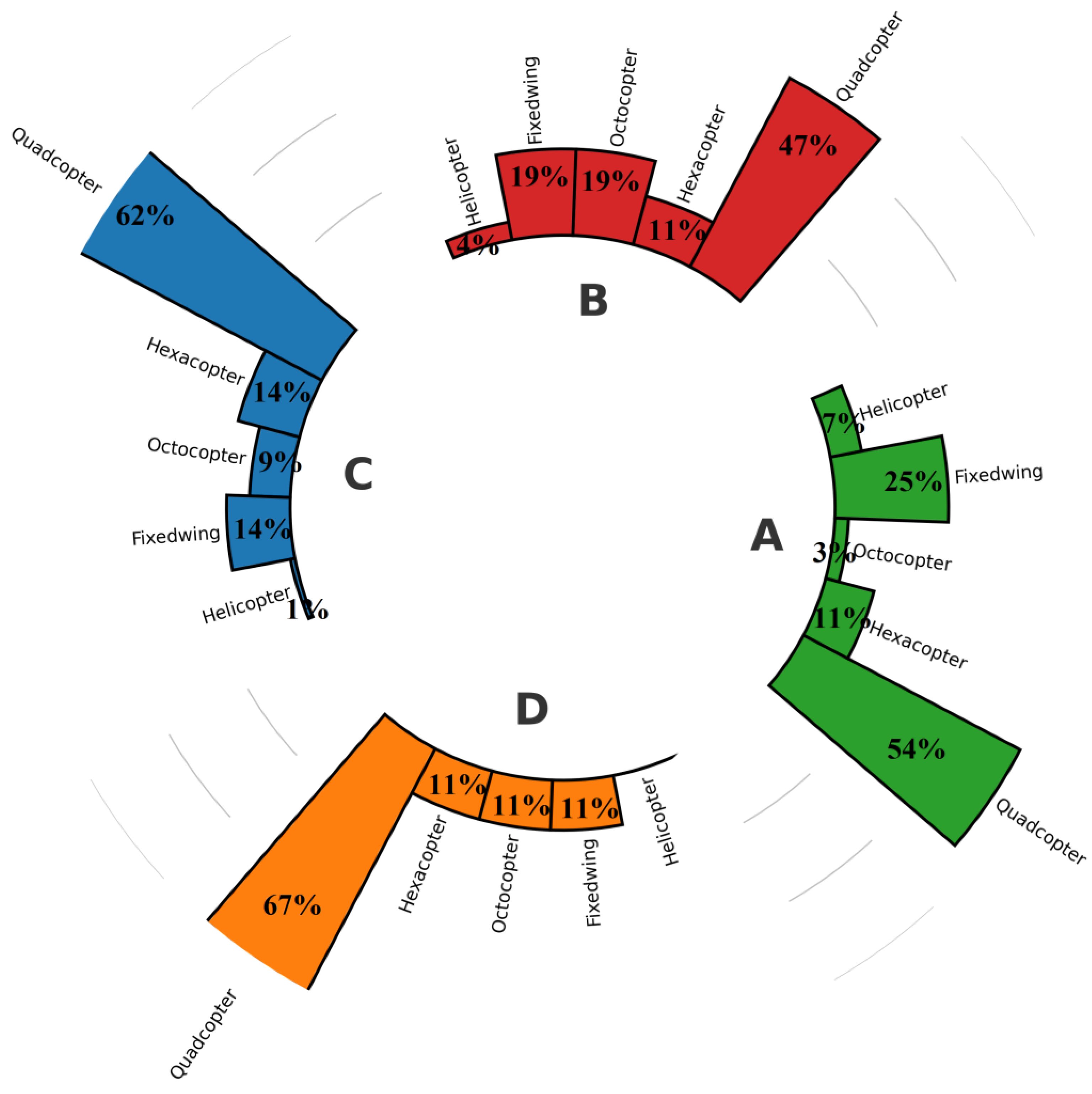
Rotary-wing and fixed-wing UASs were the most frequently used types of UASs in agricultural fields [22]. Rotary-wing UASs provide higher resolution images because they can fly in lower altitudes with lower speeds [69]. Compared with fixed-wing UASs, rotary-wing UASs cover smaller regions and take longer to fly over the same area [22]. Fixed-wing UASs need runways for takeoff and landing regions, and some are hand-launched from a launcher ramp. They can cover larger areas, and get a centimeter-level accuracy of ground sample distance because they can fly at high cruise altitudes and speeds [22]. The majority of studies considered in this review (more than 65%) reported using rotary-wing platforms to collect data, and quadcopters were the most frequently employed (45–67%) platform (Figure 2). The eBee UASs (developed by senseFly, Swiss, Switzerland) was the commonly used fixed-wing UAS to estimate the AGB [34,48,70,71,72]. It does not come as surprise that most of the studies reported using DJI drones (DJI Inc., Shenzhen, China) (Phantom 3, Phantom 4, Matrice 100, Matrice 200, and Matrice 600) as the platform of choice to carry RGB [11,17,32,73], multispectral (MS) [45,72,74,75,76,77], hyperspectral (HS) [78,79,80], and LIDAR [81,82,83] sensors. While the existing evidence [2] suggests that platform choice may not heavily impact AGB estimation accuracy, further research is needed to validate and expand upon these findings.

3.2. Sensors

UASs offer an advantage over satellites and manned aircraft in terms of the range of available sensors and the ability to perform spectral imaging, due to their close proximity to the ground [84]. The most used sensors for AGB estimation and their applications are shown in Table 3. Factors that make a sensor suitable for AGB measurement include accuracy, spectral and spatial resolution, cost, and data collection and processing complexity. RGB sensors may be sensitive to environmental factors [85], while multispectral sensors may have lower spatial resolution [86]. Hyperspectral sensors can provide detailed analysis of plant species at tissue level [87], while LIDAR sensors can be used to measure height and density of vegetation [81]. RGB and multispectral sensors are easier to use, and the data analysis is less complex than LIDAR and hyperspectral sensors [59]. LIDAR and hyperspectral sensors offer greater accuracy in capturing structural and spectral information, which is crucial for estimating AGB [88]. However, cost, dataset size, and complexity of image processing are among the drawbacks of using LIDAR and hyperspectral sensors [22].
Analyzing the sensors used in previously published papers, we observed that different types of sensors were commonly employed for AGB estimation in various ecosystems (Figure 3). LIDAR and RGB sensors were frequently utilized for AGB estimation in forest studies, where LIDAR sensors offered distinct advantages due to their ability to accurately measure the vertical growth of trees [96], reduces the saturation effect in AGB estimation [97,98], and less affecting by solar zenith angles and cloudiness [82,99]. However, in agricultural crops and grass fields, RGB, multispectral (MS), and hyperspectral (HS) sensors were more commonly used for AGB estimation. This choice of sensors in non-forest environments could be attributed to factors such as cost [100], weight [42], and the provision of more spectral information [101]. It is important to emphasize that the selection of sensors is influenced by the specific requirements and characteristics of each studied ecosystem, as well as the growth stage of the vegetation. For example, when canopy density is at its highest stage, LIDAR-derived values can cause an overestimation of biomass [83]. In the following sections, we will further explore the considerations for sensor selection and their impact on AGB estimation accuracy.

4. Importance of Flight Parameters in AGB Estimation

Careful consideration of UASs flight parameters is crucial for ensuring the effectiveness and accuracy of data collected in various applications. The importance of flight parameters setting for accurate biomass estimation was evaluated by examining the impact of different settings such as flight altitude, flight speed, and overlap on the accuracy of biomass estimation in four groups of crops.

4.1. Flight Altitude

Flying at a lower altitude reduces the size of the covered area per flight, it might results in more flights to cover a study site, and can lead to greater variability in environmental conditions affecting radiometric adjustments [35]. On the contrary, flying at a higher altitude reduces flight time and allows larger areas to be covered, helping to keep environmental conditions consistent [55]. The ground sampling distance (GSD), is defined as the physical distance on the ground represented by each pixel in an image [102]. The relationship between flight altitude and GSD is direct, according to Equation (1). Lower altitude results in a smaller GSD, meaning that the image resolution of the ground is higher. Higher altitude results in a larger GSD, meaning that the image resolution of the ground is lower. The relationship between flight altitude and GSD is defined by the camera’s field of view, lens properties, and sensor size [103].
G S D = a × h f
where h: flight altitude, f: principal distance of the lens, GSD: ground resolution, and a: pixel size. For a deeper understanding of flight altitude and its implications, the reader is referred to [55].
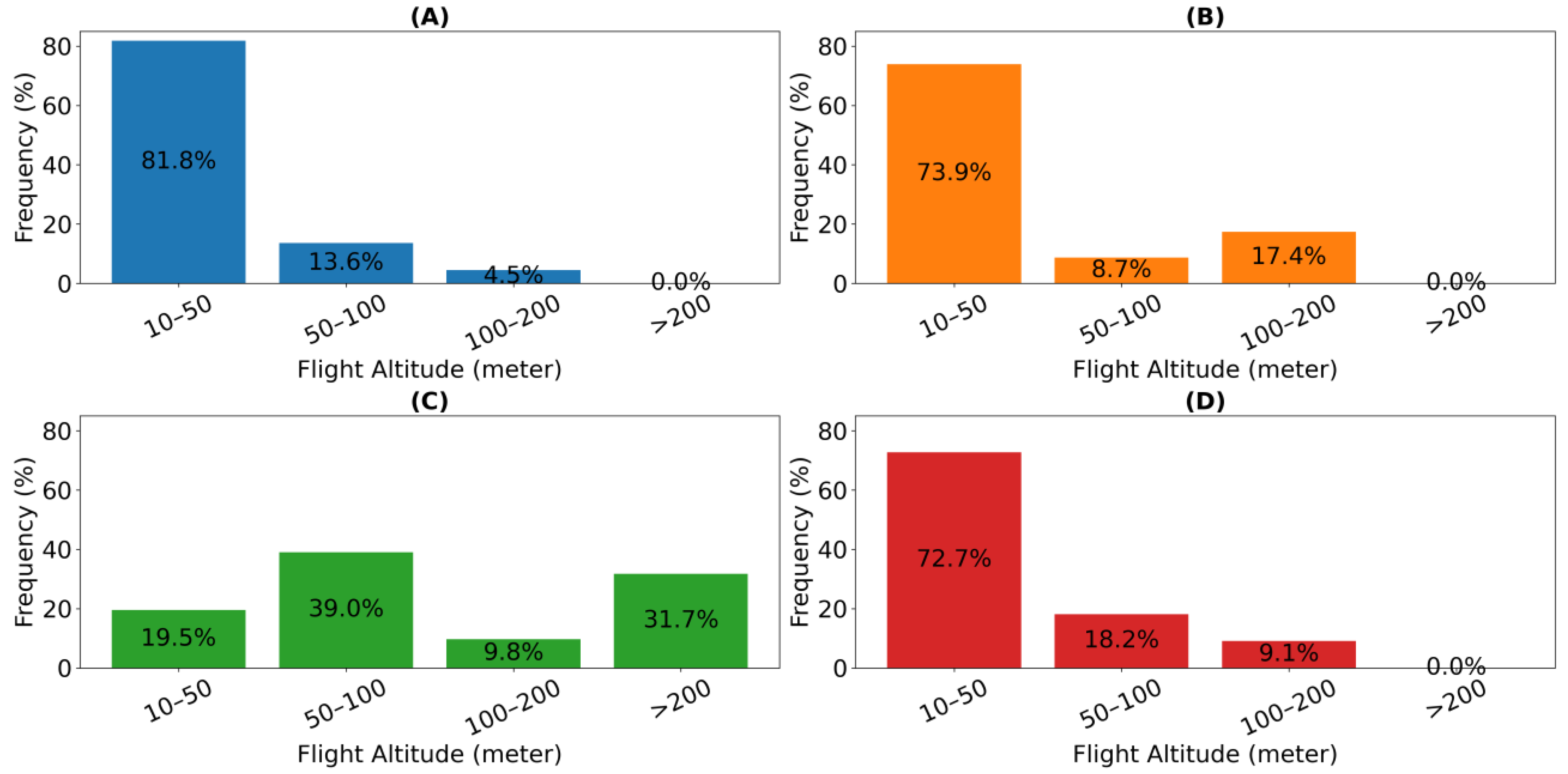
With respect to the different flight altitude classes for various vegetation types, a predominant number of flights for grasses and agricultural crops were conducted within a range of 10 to 50 m above ground level (AGL). Conversely, the highest frequency of flights was observed in the 50 m and 100 m above-ground-level classes for forests (Figure 4). This preference for lower flight altitudes can be attributed to the characteristics of the respective vegetation groups. Grasses and agricultural crops, known for their relatively low height and even surface, benefit from capturing detailed data at closer ranges. This enables a more accurate estimation of above-ground biomass. On the other hand, forests, characterized by their intricate vertical structure and potential canopy variations [104], necessitate flights at slightly higher altitudes to ensure a comprehensive capture of the biomass distribution. This is due to the need to encompass the complex three-dimensional nature of forest ecosystems, where flying at elevated altitudes provides a more encompassing perspective of the vegetation and its biomass distribution [105]. In general, the lack of standardization, limited justification for altitude selection, and the need to consider spatial resolution and minimum mapping units contribute to the variation in flight altitudes observed across different crop groups [106]. Further research and empirical studies are needed to establish best practices and guidelines for determining optimal flight altitudes and resolutions in UAS-based above-ground biomass estimation applications.
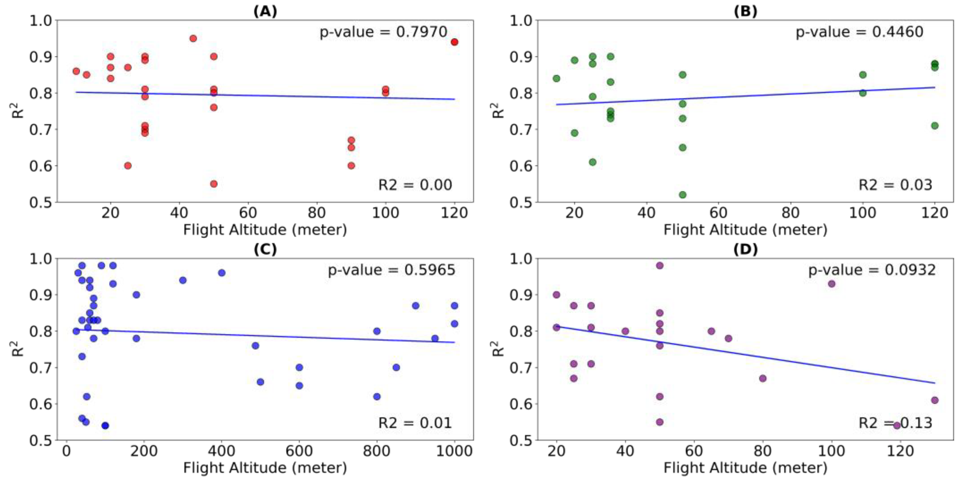
To evaluate the impact of flight altitude on the accuracy of AGB estimation, a scatter plot was generated using the values of coefficient of determination (R2) of the biomass model and flight altitude reported in four different groups of crops (Figure 5). Subsequently, a statistical analysis was performed to determine the significance of this relationship. The p-value serves as a measure of statistical significance and helps determine whether the observed relationship is likely due to chance or represents a meaningful correlation. The obtained p-values for the R2 coefficients in AGB estimation models and flight altitude across vegetation types are: 0.7970 (vertically growing crops), 0.4460 (horizontally growing crops), 0.5965 (forests), and 0.0932 (grasses). These p-values suggest that there is no statistically significant relationship between flight altitude and AGB estimation accuracy in any of the vegetation types studied, as all p-values are above the commonly used significance threshold of 0.05. Several factors might contribute to this finding. Firstly, the nature of the crops themselves could influence the relationship between flight altitude and AGB estimation accuracy. It is possible that the structural characteristics and spatial distribution of the crops minimize the impact of flight altitude on the estimation process [102]. Additionally, other variables such as data processing techniques, and environmental conditions might play a more dominant role in determining the accuracy of AGB estimation, overshadowing the influence of flight altitude. These findings show that the variation in flight altitudes within the evaluated range did not significantly affect the precision of AGB estimation. Therefore, users can fly at a higher altitude without negatively impacting the accuracy of AGB estimation. This can lead to significant time-saving benefits both during data collection in the field and data processing. However, further research is warranted to explore the potential interactions between flight altitude and other influential factors to gain a comprehensive understanding of their combined effects on AGB estimation accuracy.
Grasses show higher sensitivity to flight altitude in AGB estimation compared to other vegetation types. The p-value of 0.0932, though not statistically significant, suggests a potential trend. Factors contributing to this include the lower and more uniform canopy structure of grasses, resulting in distinct variations in AGB estimation with altitude changes. Additionally, the unique growth dynamics of grasses, including distinct growth patterns and rates, make them more responsive to altitude changes [107]. Further research is required to validate these observations.
To assess the impact of sensor type (Figure 6a), side (Figure 6b) and forward (Figure 6c) overlap on the flight altitude, a comparison was conducted between these parameters. Then, statistical analysis was conducted to calculate p-values for these comparisons. These analyses determined whether significant differences existed in the flight altitude based on the sensor type and overlap. The results of the analysis indicated that there were significant differences in the flight altitude based on the sensor type and overlap (p-value less than 0.05). It was found that in terms of above-ground biomass estimation, LIDAR has a higher average flight altitude compared to other sensors. When comparing RGB, multispectral, and hyperspectral sensors, multispectral sensors exhibited a higher flight altitude than the RGB and multispectral sensors. In addition, flights with side and forward overlap greater than 70% are typically more common at lower flight altitudes.
LIDAR sensors have the capability to operate at higher altitudes compared to other sensors due to their unique technology. LIDAR systems use laser pulses to measure distances and generate precise 3D point cloud data [95]. The laser beams emitted by LIDAR sensors have a narrow footprint and high energy, allowing them to penetrate through vegetation and capture detailed information about the terrain and objects at greater distances [108]. Additionally, lidar’s robustness against certain atmospheric conditions and signal interferences enables it to perform reliably at elevated altitudes, contributing to its suitability for high-altitude flight operations [109]. RGB sensors can be susceptible to signal interference from atmospheric conditions or surrounding objects [110]. To minimize such interference and ensure data accuracy, it may be necessary to fly at lower altitudes. In contrast, LIDAR and multispectral sensors might be less affected by these interferences, enabling them to operate at higher altitudes. One reason maybe that at lower flight altitudes, the perspective distortion is more pronounced due to the proximity of the sensor to the ground [111]. Increasing the overlap compensates for this distortion by capturing multiple images of the same area from slightly different angles, resulting in a more accurate and undistorted representation.

4.2. Flight Speed

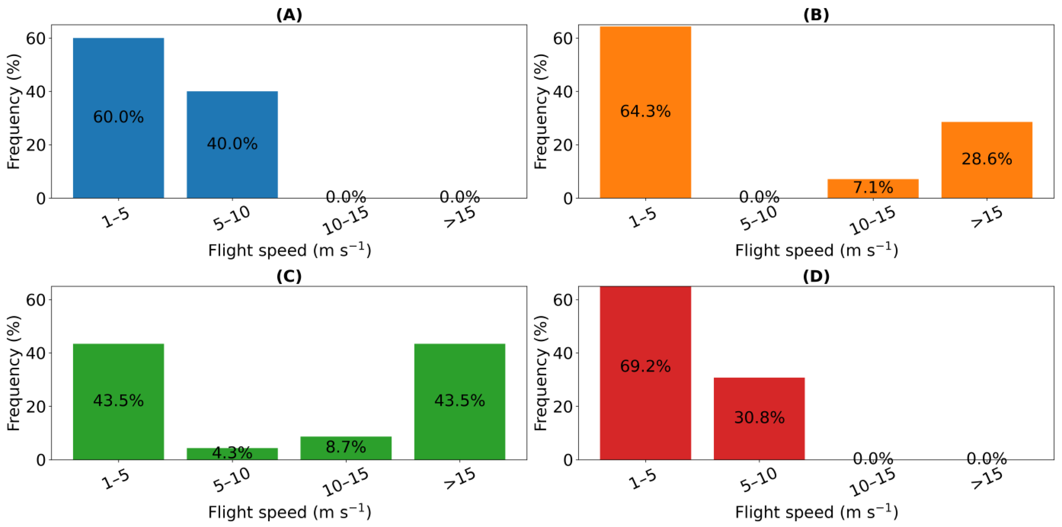
UASs can fly at a range of speeds depending on the specific model and design. Flying at a slower speed can increase the duration of the flight [112]. The high flight speed of UAS can lead to a loss of details in the images, which can make it more difficult to accurately identify and measure individual plants and other features on the ground [113]. The results indicate that the flight speed of unmanned aerial systems (UASs) varied across different vegetation types (Figure 7). The majority of flights conducted for horizontally growing crops, vertically growing crops, and grasses occurred at speeds between 1 and 5 m per second (m s−1), with frequencies of 60%, 64.3%, and 69.2%, respectively. In contrast, forests exhibited a more balanced distribution of flight speeds, with approximately equal frequencies in the 1–5 m s−1 and greater than 15 m s−1 categories. This suggests that the flight speed preference is influenced by the characteristics of the vegetation types.
The variation in flight speeds across different vegetation groups for above-ground biomass (AGB) estimation can be explained by several factors. Vegetation structure and density influence the flight speed preferences, with horizontally growing crops favoring lower speeds (1–5 m s−1) due to their uniform and dense canopies, while vertically growing crops require higher speeds (>15 m s−1) to capture their vertical structure and cover larger areas efficiently. Sensing resolution and image quality also play a role, as slower speeds enable higher-resolution imagery for accurate identification and measurement of individual plants [114], particularly in grasses and vertically growing crops. Environmental factors, including wind speed and turbulence, influence flight speed choices to maintain stability and image clarity [115], with higher speeds (>15 m s−1) preferred in forests to mitigate the impact of wind. Higher flight speeds enable the LIDAR sensor to capture more data points per unit area, creating a denser point cloud for a detailed representation of the forest’s structure [43]. This is crucial for comprehensive forest analysis, as forests cover large areas, and higher speeds allow for faster data collection, reducing survey time.
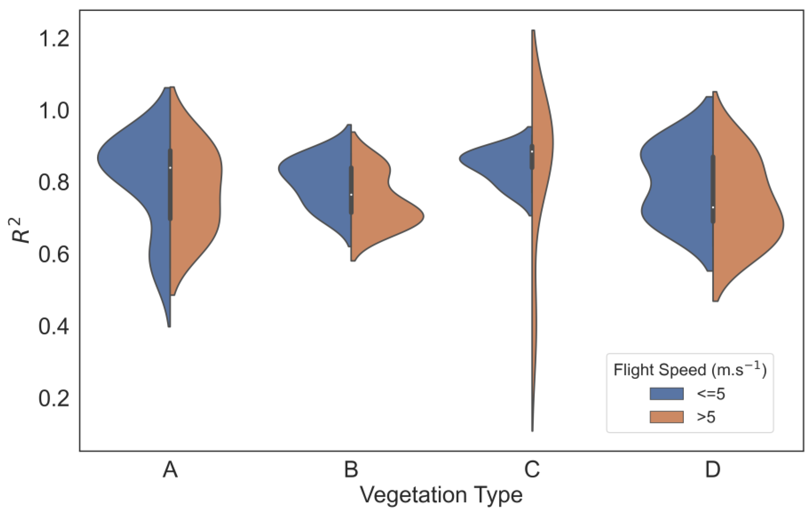
The impact of flight speed on the accuracy of AGB estimation was assessed by dividing the studies into two categories based on flight speed, below 5 m s−1 and above 5 m s−1. The final values of the coefficient of determination for AGB estimation were compared (Figure 8). The t-test was employed to assess whether there exists a significant difference in the accuracy of above-ground biomass (AGB) estimation between the two groups categorized by flight speed within each vegetation type. The analysis of t-test results revealed that flight speed has a statistically significant impact on the accuracy of above-ground biomass (AGB) estimation in certain vegetation types. Specifically, the t-test results showed that the p-values for grasses (p = 0.049) and horizontally growing crops (p = 0.006) were below the significance level of 0.05, indicating a significant difference in AGB estimation accuracy between the two flight speed groups. However, for forests (p = 0.229) and vertically growing crops (p = 0.701), the p-values were above 0.05, suggesting that the difference in flight speed did not have a significant impact on AGB estimation accuracy in these vegetation types.
The importance of flight speed in grasses and horizontally growing crops for above-ground biomass (AGB) estimation can be attributed to several factors. These vegetation types have a more uniform structure, making them susceptible to variations in flight speed that can affect sensor resolution, signal penetration, and the capture of fine-scale details relevant to AGB estimation. The lower sampling density associated with higher flight speeds [116] can also hinder accurate AGB estimation in grasses and horizontally growing crops, as these vegetation types require finer-scale data. In contrast, the denser and more heterogeneous structures of forests and vertically growing crops may minimize the impact of flight speed on AGB estimation accuracy due to structural variations or the need for higher sampling densities regardless of flight speed. Generally, faster flight underestimated biomass compared to standard settings by negatively impacting on the data’s coverage and resolution [116].
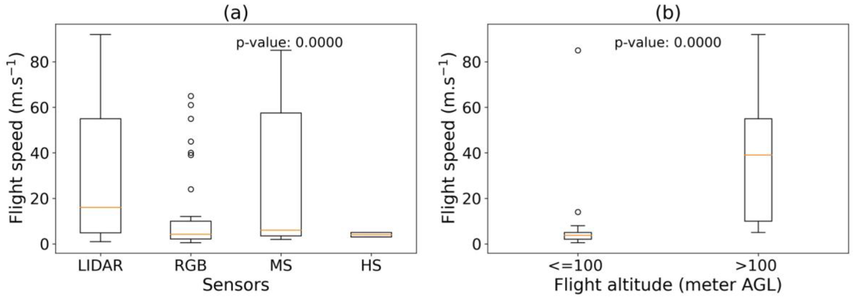
To assess the impact of sensor type (Figure 9a) and flight altitude (Figure 9b) on the flight speed, a comparison was conducted between these parameters. Then, statistical analysis was conducted to calculate p-values for this comparison. The results indicated a significant difference in flight speed among various sensors (LIDAR, RGB, multispectral, hyperspectral) and flight altitudes (below and above 100 m AGL). On average, LIDAR and multispectral sensors exhibited higher flight speeds compared to RGB and hyperspectral sensors. Flights conducted at altitudes above 100 m AGL demonstrated greater flight speeds compared to flights at altitudes below 100 m AGL. The higher resolution and data complexity of RGB and hyperspectral sensors may necessitate slower flight speeds for accurate data collection, leading to lower overall flight speeds. Flights at altitudes above 100 m AGL may prioritize broader coverage or time-sensitive data acquisition, resulting in increased flight speeds to efficiently cover larger areas.

4.3. Image Overlaps

Overlap refers to the percentage by which each image overlaps with its neighboring images. Small overlaps can decrease the number of flights and, thus, reduce the flight costs [113]. A higher overlap allows for more accurate stereo processing [117], which can result in a heavy dataset and increasing the time of process.
Regarding the percentage of image overlap, horizontally growing crops had the highest frequency (60%) in the 75–85% overlap range, indicating consistent image coverage. Figure 10 presents the frequency distribution of forward overlap classes used for different vegetation types. The distribution of side overlap exhibited similar patterns; hence, a single figure was utilized to represent both overlap types. Vertically growing crops had a more varied distribution, with roughly equal frequencies (23.8%) across the 50–60%, 60–75%, 75–85%, and >85% overlap ranges. Forests predominantly fell in the 75–85% overlap range (52.4%), while grasses had a majority (56.2%) in the 75–85% overlap range. These findings highlight the variability in image overlap characteristics among different vegetation types. The observed differences in image overlap characteristics among different vegetation types can be attributed to several factors. One significant factor is the limitations of the platform used for data collection, which can influence the selection of the desired overlap. For instance, fixed-wing platforms are generally unable to fly at low speeds and altitudes required to achieve sufficient overlap with this specific sensor. These limitations can hinder the ability of fixed-wing platforms to capture the desired level of sensor overlap effectively [106]. Secondly, the selection of overlap is dependent on the type of sensor used in the study. For instance, when utilizing LIDAR sensors to measure plant height, some studies [25,43,118,119,120] have considered lower overlap percentages ranging from 50% to 60%. On the other hand, when using multispectral sensors to calculate vegetation indices, other studies [75,121,122,123] have opted for higher overlap percentages, typically around 75% to 85%.
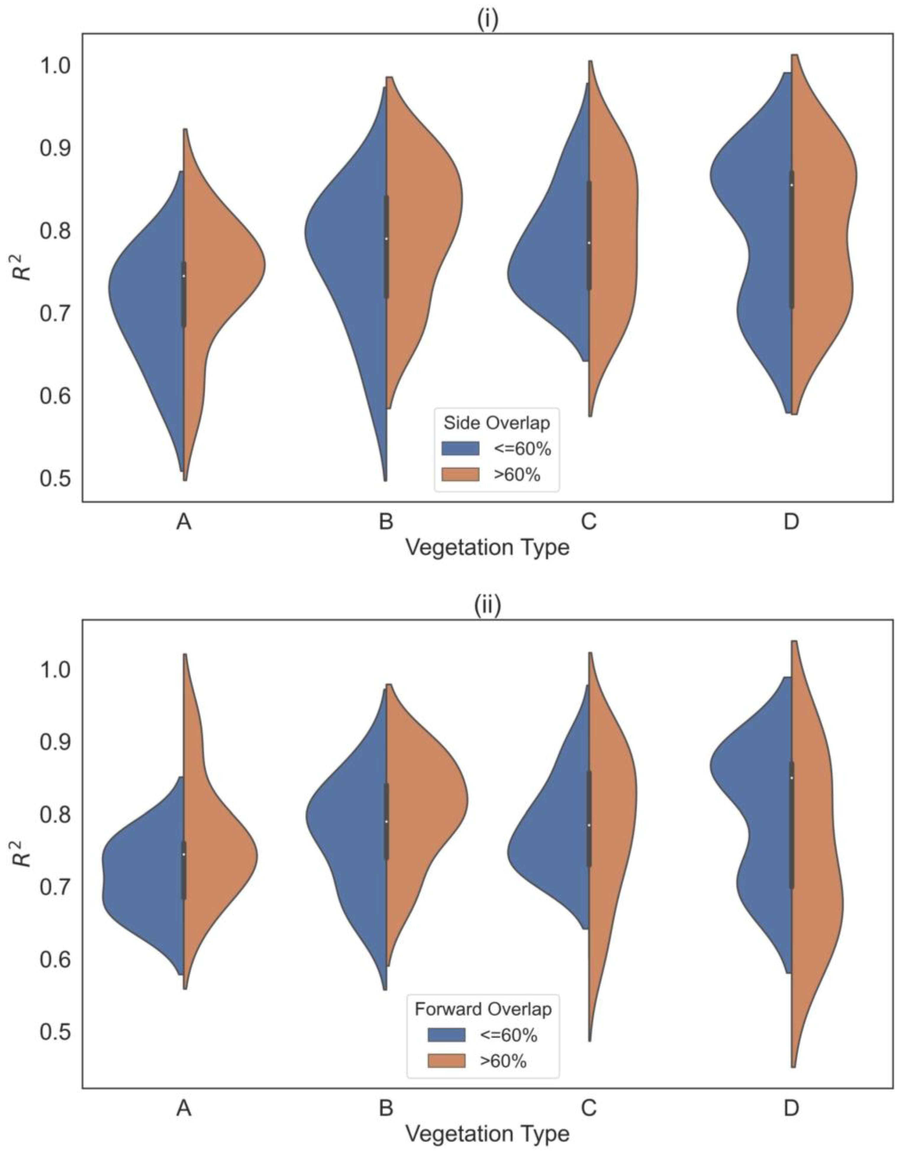
To evaluate the effect of overlap percentage on the accuracy of biomass estimation, two groups of side (Figure 11i) and forward (Figure 11ii) overlap (less and greater than 60%) for all categories of plants were assessed based on the final values of R2 of the studies.
For the forest vegetation type, the p-values for side overlap and forward overlap were 0.1547 and 0.0222, respectively. The relatively low p-value for the forward overlap suggests a statistically significant impact on biomass estimation accuracy, indicating that greater than 60% forward overlap leads to improved results. The significant impact of forward overlap on biomass estimation accuracy in forest vegetation can be attributed to the requirements of the Structure from Motion (SfM) workflow commonly employed in the analyzed studies. SfM algorithms rely on a large number of overlapping images to identify key points and create 3D point clouds for surface models [106].
In the case of grasses, the p-values for side overlap and forward overlap were 0.9073 and 0.2228, respectively. Both p-values were above the significance level of 0.05, indicating that the choice of overlap percentage did not have a significant impact on biomass estimation accuracy for this vegetation type. For horizontally growing crops, the p-values for side overlap and forward overlap were 0.6532 and 0.1450, respectively. Similar to grasses, neither p-value was below the significance level, indicating that the selection of overlap percentage did not significantly influence biomass estimation accuracy in horizontally growing crops. In the case of vertically growing crops, the p-values for side overlap and forward overlap were 0.7815 and 0.8275, respectively. Both p-values were above 0.05, indicating that the choice of overlap percentage did not have a significant impact on biomass estimation accuracy in vertically growing crops.
Overall, having a higher forward overlap is more important for a better AGB estimation in forests compared to side overlap. Consequently, it may be a cost-effective solution to decrease the side overlap while maintaining a constant forward overlap to minimize the flight time and acquisition expenses. For grasses, horizontally growing crops, and vertically growing crops, the impact of overlap percentage on biomass estimation accuracy appears to be less significant. So, operators may opt to decrease the amount of overlap to reduce flight times and minimize the volume of data that needs to be stored. Further studies may be necessary to determine the optimal value for overlap based on the flight duration and dataset size. However, based on the literature on UAS imagery collection, an overlap range of 75–85% is suggested for accurate estimation of above-ground biomass in forests, grasses, horizontally and vertically growing crops.
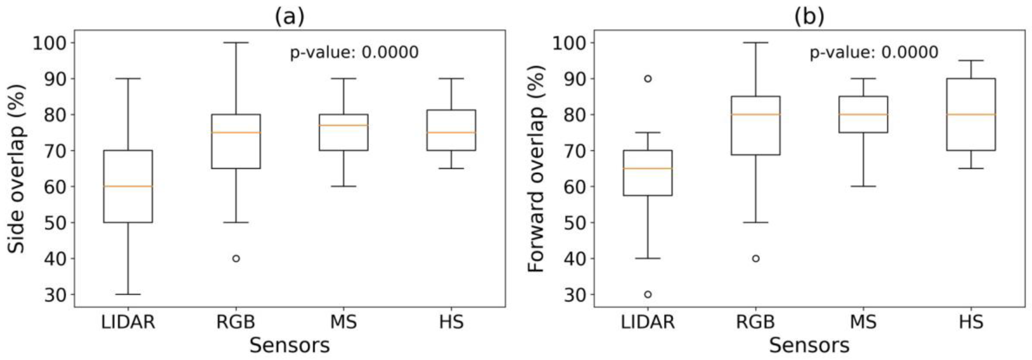
To assess the impact of sensor type on the side (Figure 12a) and forward (Figure 12b) overlap, a comparison was conducted between these parameters. Then, statistical analysis was conducted to calculate p-values for these comparisons. The results indicated a significant difference in forward and side overlap among various sensors (LIDAR, RGB, multispectral, hyperspectral). Hyperspectral, multispectral, and RGB sensors typically require both side and forward overlap greater than LIDAR sensors for accurate above-ground biomass estimation. This can be due to the fact that LIDAR sensors provide accurate 3D point clouds, which can be less sensitive to overlap variations compared to 2D imagery from hyperspectral, multispectral, and RGB sensors [124]. In addition, across all sensor types, the average forward overlap is higher than the side overlap. One reason maybe that forward overlap helps compensate for perspective distortion caused by the sensor’s nadir view angle [124]. It ensures better coverage of features in the scene, especially in areas where distortion is more pronounced.

5. Ground Control Points (GCPs)

GCPs are physical markers placed on the ground that can be used to georeference, geo-correct, and co-register images captured by the UASs [17,125,126]. By using GCPs, it is possible to accurately map the images onto a specific location on the Earth’s surface to reduce the planimetry error [14,127], which is essential for generating accurate biomass estimates. The geometric correction error of the image should be less than 0.5 pixels [103]. High-accuracy Global Navigation Satellite System (GNSS) techniques such as Real-Time Kinematic (RTK) or Post-Processed Kinematic (PPK) are often used to collect and use an appropriate number of GCPs in order to accurately georeference the data collected during the mission [65,103]. Factors such as flight altitude, study area, and complexity of the topography determine the number of GCPs per hectare [65].
It was found that the usage of 5–10 GCPs was the most prevalent among all the crop groups. Additionally, studies conducted on grasses were observed to have used a higher number of GCPs compared to other vegetation groups (Figure 13).
The higher use of Ground Control Points (GCPs) in grass studies compared to other vegetation groups can be attributed to the unique topographic characteristics of grasses. Grasses exhibit significant topographic variations, and a larger number of GCPs is required to adequately capture these variations [106]. Grasses have a complex and heterogeneous structure, with variations in height, density, and spatial arrangement. Their low-growing nature and diverse species result in intricate topographic variations. To accurately estimate biomass in grasses, more GCPs are used to capture elevation and topographic features effectively.
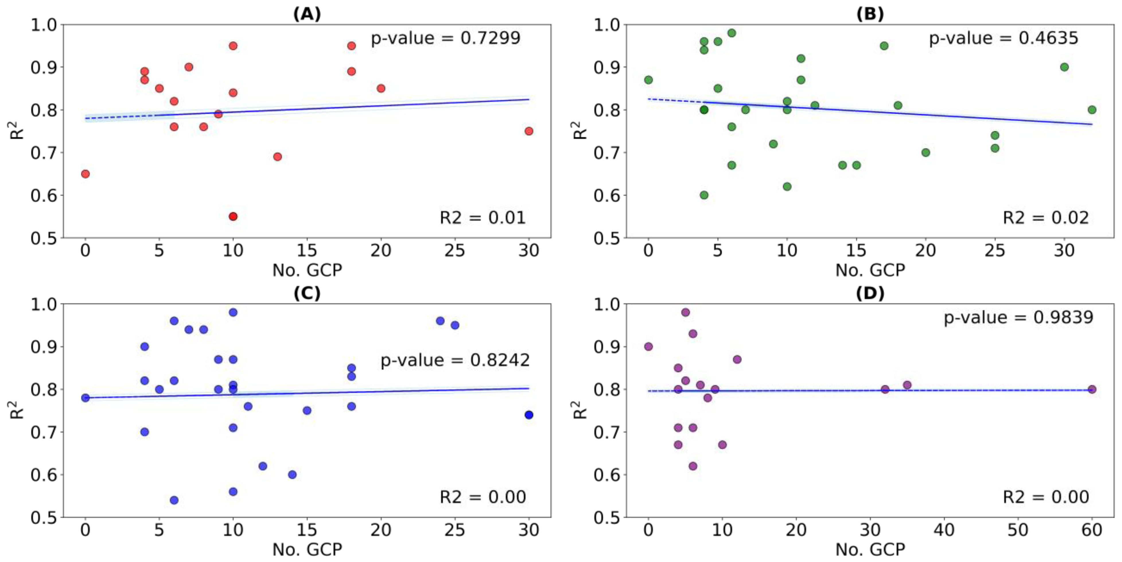
An analysis was conducted to examine the correlation between the number of GCPs and the overall accuracy of the AGB estimation model. The relationship between the number of GCPs and R2 was evaluated through the implementation of a statistical analysis (Figure 14). The results indicated that an increase in the number of GCPs does not have a significant effect on the final accuracy of the AGB estimation model. Advancements in technology, including portable and reusable GCPs with GNSS receivers and automated GCP identification and image registration techniques including sensor fusion-based registration, elastic registration, and direct image-to-image registration, have streamlined the georeferencing process. These innovations reduce the effort associated with GCP placement and measurement, and potentially enable accurate georeferencing with fewer GCPs.
To assess the impact of sensor type (Figure 15a), flight speed (Figure 15b), and flight altitude (Figure 15c) on the number of GCPs, a comparison was conducted between these parameters. Then, statistical analysis was conducted to calculate p-values for each comparison. The results of the analysis indicated that there were significant differences in the number of GCPs based on sensor types (p-value less than 0.05). Specifically, it was found that the average number of GCPs increased when LIDAR was used. In terms of flight speed and altitude, there were no significance difference between the number of GCPs at different flight speed (p-value = 0.4684) and altitude (p-value = 0.9784). A higher flight speed was associated with less variation in the number of GCPs. Lastly, when considering flight altitude, it was observed that the average number of GCPs was higher for flight heights above 100 m above ground level (AGL) compared to heights below 100 m AGL.
The significant differences in the number of GCPs at different sensors can be attributed to the fact that the use of LIDAR technology requires a higher average number of GCPs [128], indicating its specific requirements for accurate georeferencing.
Table 4 highlights the key flight parameters, the expected resolution for that specific flight parameters, and the number of GCPs to estimate AGB in different groups of vegetation. LIDAR sensors show a wider range of flight altitude and speed, especially for forest and vertically growing crops. MS and HS sensors demonstrate a wider range of flight altitude and speed in vertically growing agricultural crops compared with RGB sensors. LIDAR sensors need less side and forward overlap compared to RGB, MS, and HS sensors and RGB sensors need more overlap than MS sensors.

6. Data Acquisition Time

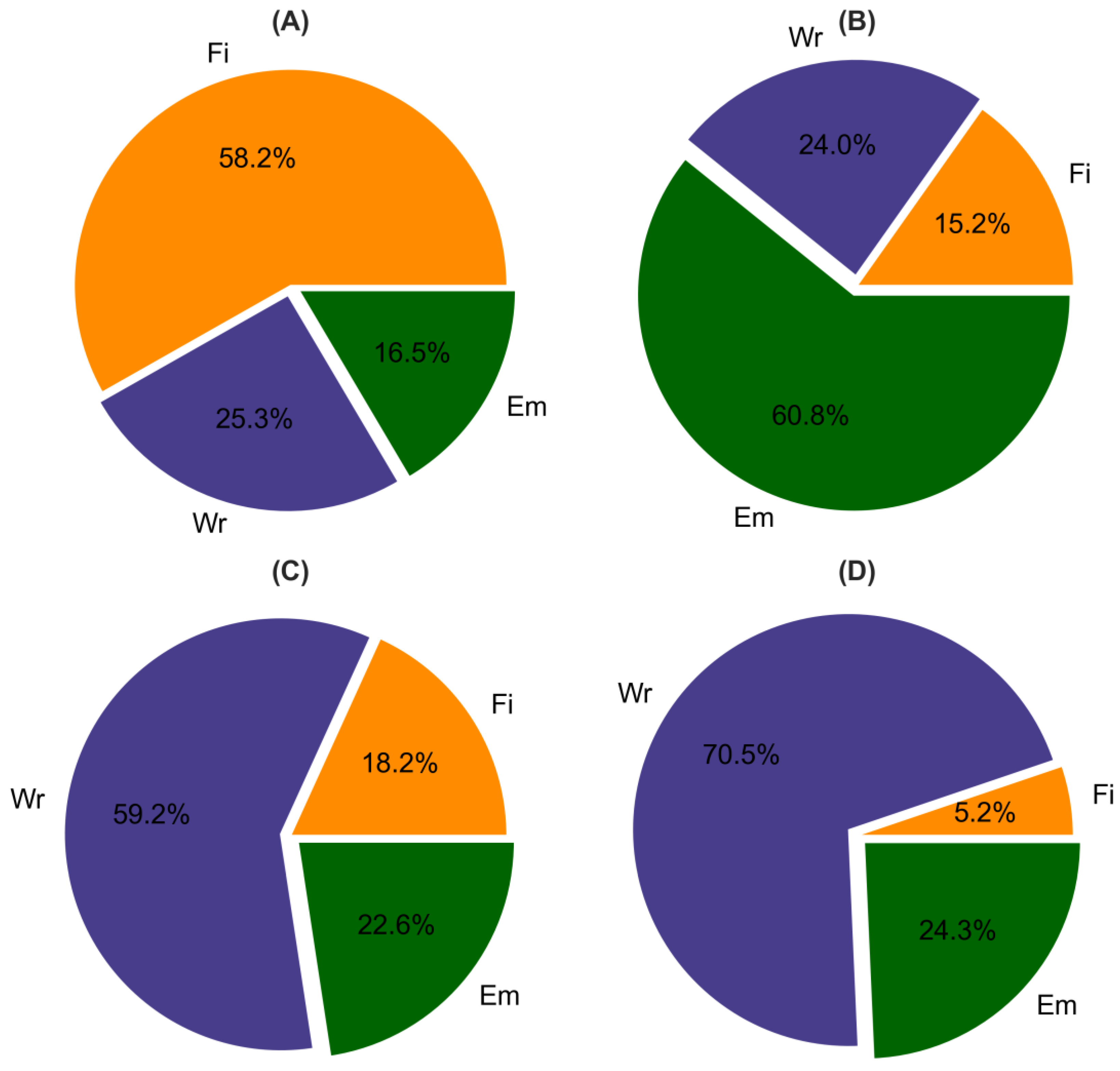
The time at which the UAS is used to collect data, can influence the accuracy of AGB estimation by changing the illumination conditions [65,171,177], reducing the effect of water content [178], reducing the effect of shadow [79,179], and reducing the effect of wind [40]. The solar noon helps to maintain a minimum solar angle of 50° from the horizon, which improves image quality, increases solar energy availability, and reduces atmospheric effects [15,35,171]. The early and late time in the day is not a good time to fly because at these times the leaf’s water content, which reduces the amount of reflectance, is high and could reduce the AGB estimation accuracy [178]. Wind speed that has a direct effect on the accuracy of imaging through UAS stability and plant movement can change during different times of the day. Moving the UASs due to wind during imaging can make it impossible to obtain a clear orthomosaic image and cause stillness and blurring on the image [40]. Displacement of the plant due to wind speed reduces the quality of the image dataset especially regarding spectral and structural information because plant movement leads to change in canopy structure [180]. Figure 16 shows the frequency of different times of the day with respect to flight in AGB estimation studies. According to this figure more than 50% of AGB estimation-related flights for all groups of vegetation were performed between 12:00 and 2:00 pm.

7. Importance of Modeling Factors in AGB Estimation

The accuracy and predictive ability of AGB estimation using UAS imagery depends on the choice of the parameter(s) derived from the imagery [2]. In this study, we focused on the importance of the number of vegetation indices, types of textural and structural metrics of vegetation, feature selection, and choice of predictor algorithm to estimate the AGB.

7.1. Vegetation Traits

7.1.1. Vegetation Indices (VIs)

RGB vegetation indices are useful for estimating AGB using UASs imagery [65]. They can estimate AGB by measuring chlorophyll in leaves [181]. Chlorophyll in leaves is related to the plant’s ability to produce biomass [182]. Near-infrared (NIR) and red edge vegetation indices are commonly used in estimating biomass in vegetation. NIR vegetation indices are based on the reflectance of near-infrared wavelengths by vegetation, which is higher in healthy vegetation than in unhealthy or senescent vegetation [34,42]. Visible and NIR bands are highly sensitive to low biomass, thus, a simple combination of these bands can create a good estimation of vegetation biomass [73]. Red edge vegetation indices use reflectance of light in the red edge spectral range (700–740 nm) to estimate the amount of vegetation per unit of area [183]. They show a stronger association with leaf biomass compared to stem biomass [2,45,157]. For a comprehensive understanding of the prevalent RGB, NIR and red edge vegetation indices to AGB estimation please refer to Poley and McDermid [2].
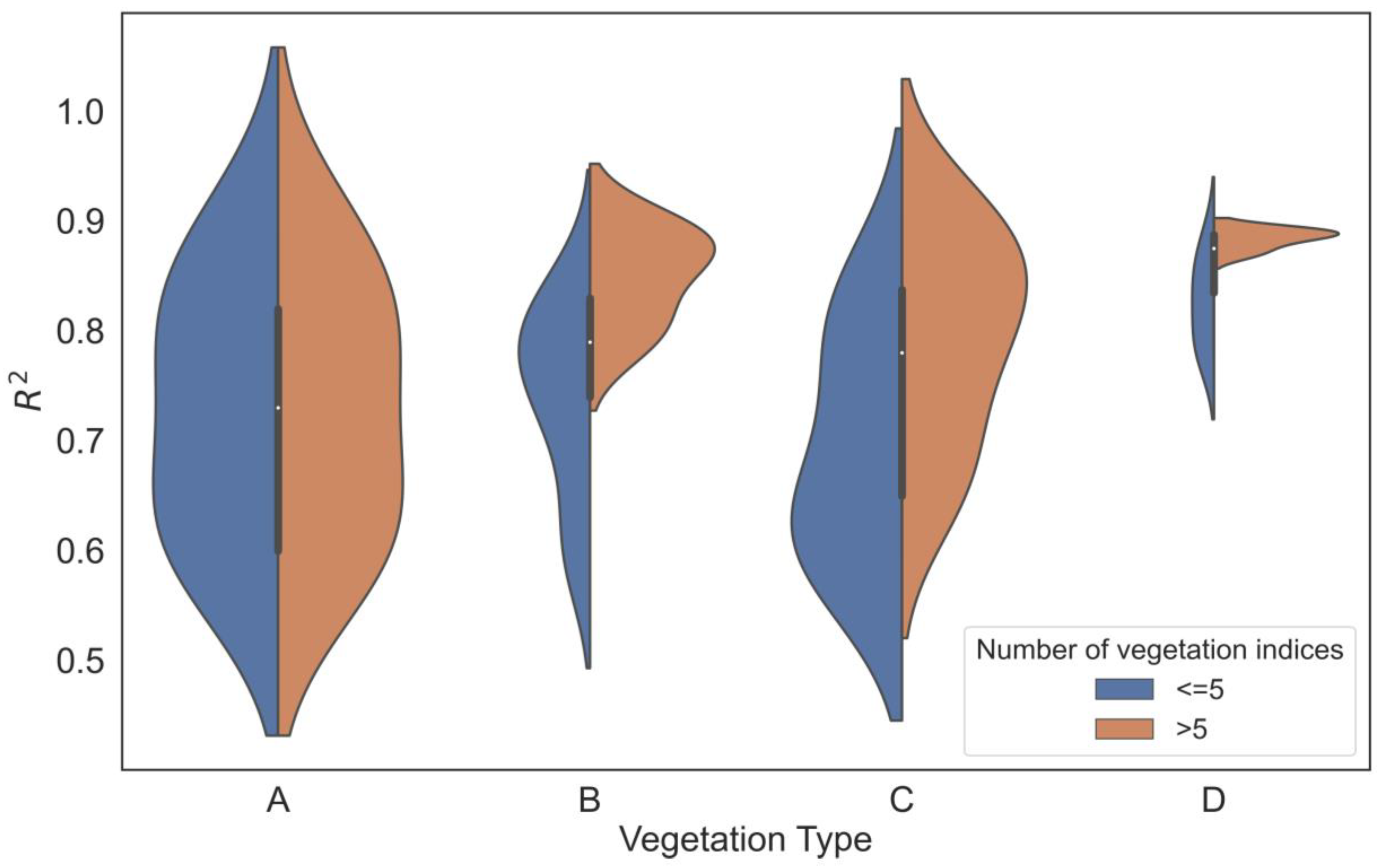
We examined the impact of the quantity of vegetation indices on the accuracy of AGB estimation by doing a statistical analysis. The results are presented in Figure 17, with the AGB accuracy of models using different numbers of vegetation indices (less than or equal to 5 and greater than 5) for various vegetation groups. The impact of the number of vegetation indices on AGB estimation accuracy varied across different vegetation types. For forests, the p-value of 1 indicated no statistically significant impact. The structural variations within forests may overshadow the specific impact of the number of vegetation indices on AGB estimation. Similarly, for grasses, the p-value of 6.4758 indicated a lack of statistical significance. Horizontally growing crops had a p-value of 3.403, also suggesting no significant impact. Grasses and horizontally growing crops often have a more homogeneous structure compared to other vegetation types [184]. This uniformity in structure may lead to less variability in AGB estimation accuracy, resulting in a lack of statistical significance for the number of vegetation indices due to the consistent signal response, limited structural complexity, and homogeneous growth conditions. However, vertically growing crops showed a significantly low p-value of 0.0007, indicating that the number of vegetation indices had a significant impact on AGB estimation accuracy in this vegetation type. Vertically growing crops, such as corn or wheat, often have complex and variable structures, with variations in plant height and canopy density. The number and selection of appropriate vegetation indices can capture these structural differences, leading to improved AGB estimation accuracy.

7.1.2. Vegetation Texture

Several studies concluded that including image textural metrics can improve the accuracy of AGB estimation in different vegetation types [2,159,185,186]. Image texture can be used to analyze patterns and structures present in images of vegetation to extract information about the density, arrangement, and composition of the plant material [2,63]. This can be performed by analyzing the spectral and spatial variability of the grey level values in the image and comparing them to known values for different types of vegetation [187]. Image textural metrics can help to mitigate the issue of underestimating AGB at high biomass values when using vegetation indices (VIs) alone [2]. Texture parameters derived from red edge and NIR bands have been found to have a wider variation throughout the growing season, and thus can explain the greater variation in AGB than visible bands [72]. Table 5 provides a summary of the methods and their corresponding descriptions used for texture analysis in our study. These methods encompass various aspects such as co-occurrence matrix, Gabor filters, Local Binary Patterns (LBP), and Fractal Dimension. The co-occurrence matrix measures uniformity, entropy, contrast, homogeneity, and correlation in the grey level distribution of an image. Gabor filters analyze the frequency, orientation, and scale of patterns present in an image. LBP examines different types of transitions and intensity values between pixels. Lastly, fractal dimension explores the box-counting, information, and Hausdorff dimensions to assess image characteristics. These methods and types of image textural metrics have been demonstrated to be particularly useful in the estimation of biomass.

7.1.3. Structural Variables

Studies have shown that models including structural features have better accuracy in estimating AGB in various vegetation types [13,45,73,103,186]. Metrics such as tree diameter at breast height (DBH) are closely correlated with the amount of woody tissue in a tree [133,198,199,200,201], and plant height is closely correlated with vegetation growth [13,45,47] and biomass [32,202].
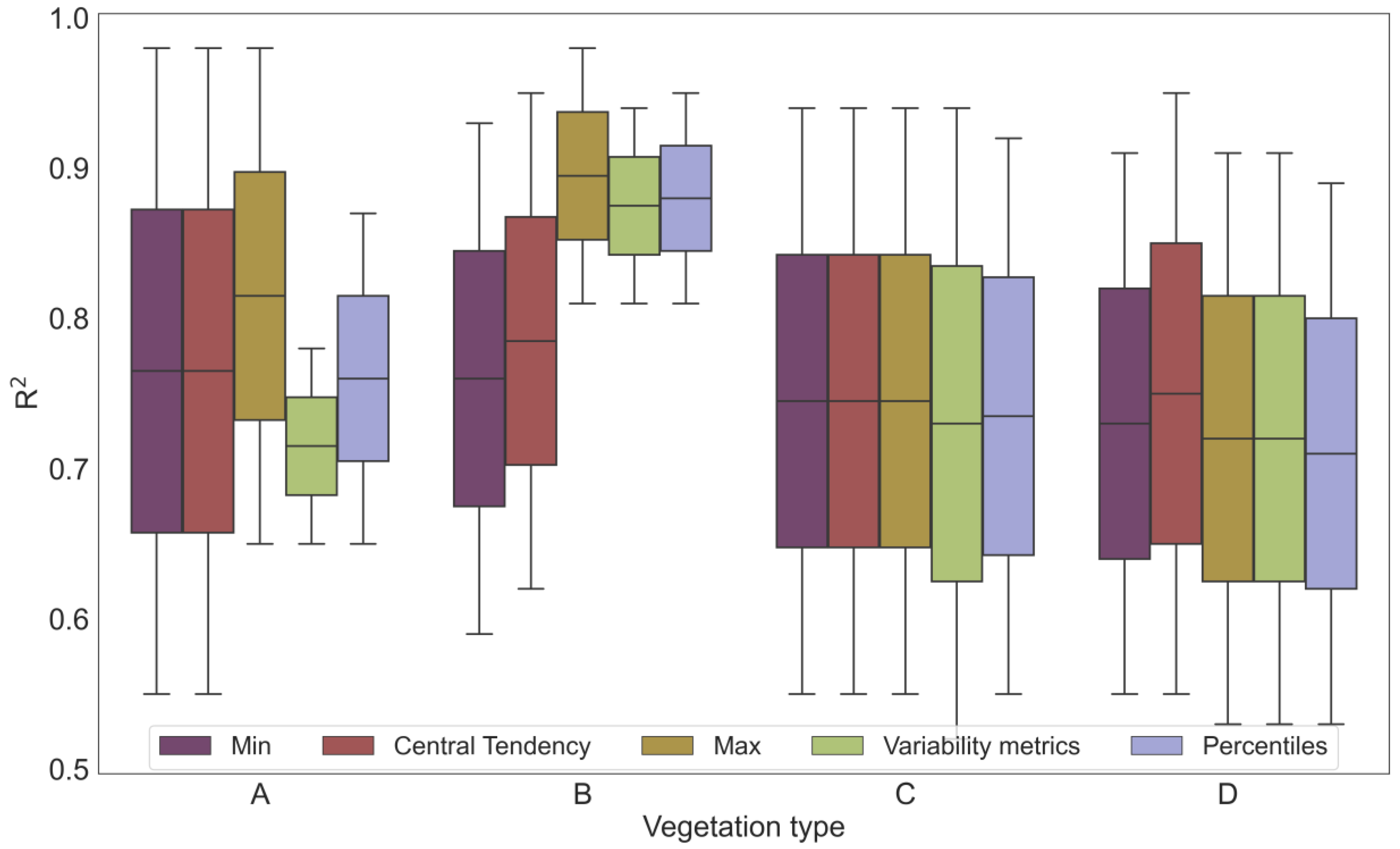
Central tendency metrics (mean, median, and mode), minimum (Min), maximum (Max), variability metrics (standard deviation, skewness, kurtosis, and variance) and percentiles of plant height are the commonly used metrics to estimate biomass. Central tendency metrics are useful for estimating overall biomass [35,45] and they are less affected by environmental noises such as the soil background [121], while measuring minimum and maximum plant height helps to identify small [104,164] or dominant [83,177,203] plants. The maximum plant height can reduce the impact of lodging on measurements of plant height [15]. Variability metrics can be used to understand variability in plant size [45,104] and finding outliers [45,104]. Percentiles aid understanding the overall shape of the distribution of plant sizes and identify any trends or patterns that may be relevant for biomass estimation [30,162,204].
Figure 18 shows the frequency of using different plant height metrics to estimate biomass in different groups of vegetation. While the maximum value of plant heights is the most used metrics to estimate the biomass in forests and vertically growing crops, the central tendency metrics of plant height are most useful for grasses and horizontally growing crops. The reason for using the maximum value of plant height in estimating biomass for forests and vertically growing crops is because the tallest plants in these vegetation types have a substantial impact on the overall biomass [205]. By considering the maximum value, capturing the highest plant height would be possible, which helps account for the influence of these tall individuals on biomass estimates. In contrast, when estimating biomass in grasses and horizontally growing crops, central tendency metrics of plant height (such as mean or median height) are more valuable. These metrics provide information about the average or typical height within these vegetation types, giving insights into the overall distribution and structure of the plants. In grasses, which often have dense and uniform canopies [38], the average height serves as a representative measure of biomass across the field. Likewise, horizontally growing crops with their spreading growth pattern [206] can benefit from central tendency metrics to capture the average height across the vegetation area.

7.2. Feature Selection

In the context of estimating AGB, feature selection can improve the accuracy of the prediction model [207] by avoiding overfitting when a variety of RGB and MS vegetation index, textural, and structural metrics are used as predictor variables [208,209] and by reducing the complexity of the model through removing unnecessary or redundant predictors [210]. Several methods are used for feature selection, including:
Filter methods: These methods use statistical tests or simple heuristics to identify features that are correlated with the target variable. They are generally fast and simple to implement, but they do not consider the interactions between features [211]. Common filter methods include variance inflation factor (VIF), Pearson’s correlation coefficient, mutual information, ANOVA f-value, chi-squared test, and variance threshold [26,186,211,212,213,214,215,216,217].
Wrapper methods: These methods use a search algorithm, such as Forward Selection (FS), Backward Elimination (BE), Recursive Feature Elimination (RFE), and Genetic Algorithms (GA) to find the optimal subset of features. They are more computationally expensive than filter methods, but they consider the interactions between features [207,210,211,218].
Embedded methods: These methods are built into the machine learning algorithm itself and select features as part of the model training process. They can be computationally expensive, but they can be effective for high-dimensional datasets. The most common embedded methods include principal component analysis (PCA), Lasso Regression, Ridge Regression, Elastic Net, Tree-Based Models, and Boosting models [207,207,219,220,221]. Figure 19 shows the frequency distribution of different feature selection methods used for above-ground biomass (AGB) estimation. Our study findings reveal that the most employed filter, wrapper, and embedded feature selection methods for AGB estimation across all vegetation groups are VIF, PCA, and BE, respectively.

7.3. Model Selection

Model selection plays a crucial role in determining the accuracy of AGB estimation since different models have varying abilities to capture the complex relationships between variables [198,222]. Complex models may capture more details but may also require more data and be prone to errors [7]. Simpler models may be easier to use but may also be less accurate [187]. AGB estimation involves many different models with unique strengths and weaknesses. Table 6 compares the main parameters, advantages, and disadvantages of commonly used models. Traditional linear regression models may have limitations in dealing with outliers, non-linearity, and multivariate data [103], while machine learning techniques such as random forest (RF) and support vector machine (SVM) have the capacity to handle multidimensional data [223,224].
Assessing a model through evaluation metrics ensures its accuracy and reliability and helps identify areas for improvement [90,178]. Mean absolute error (MAE) [34,154,232], mean squared error (MSE) [142], root mean squared error (RMSE) [159,233], coefficient of determination (R2) [32,234], and Nash–Sutcliffe efficiency (NSE) [65,235] are commonly used evaluation metrics to evaluate the performance of AGB estimation models.
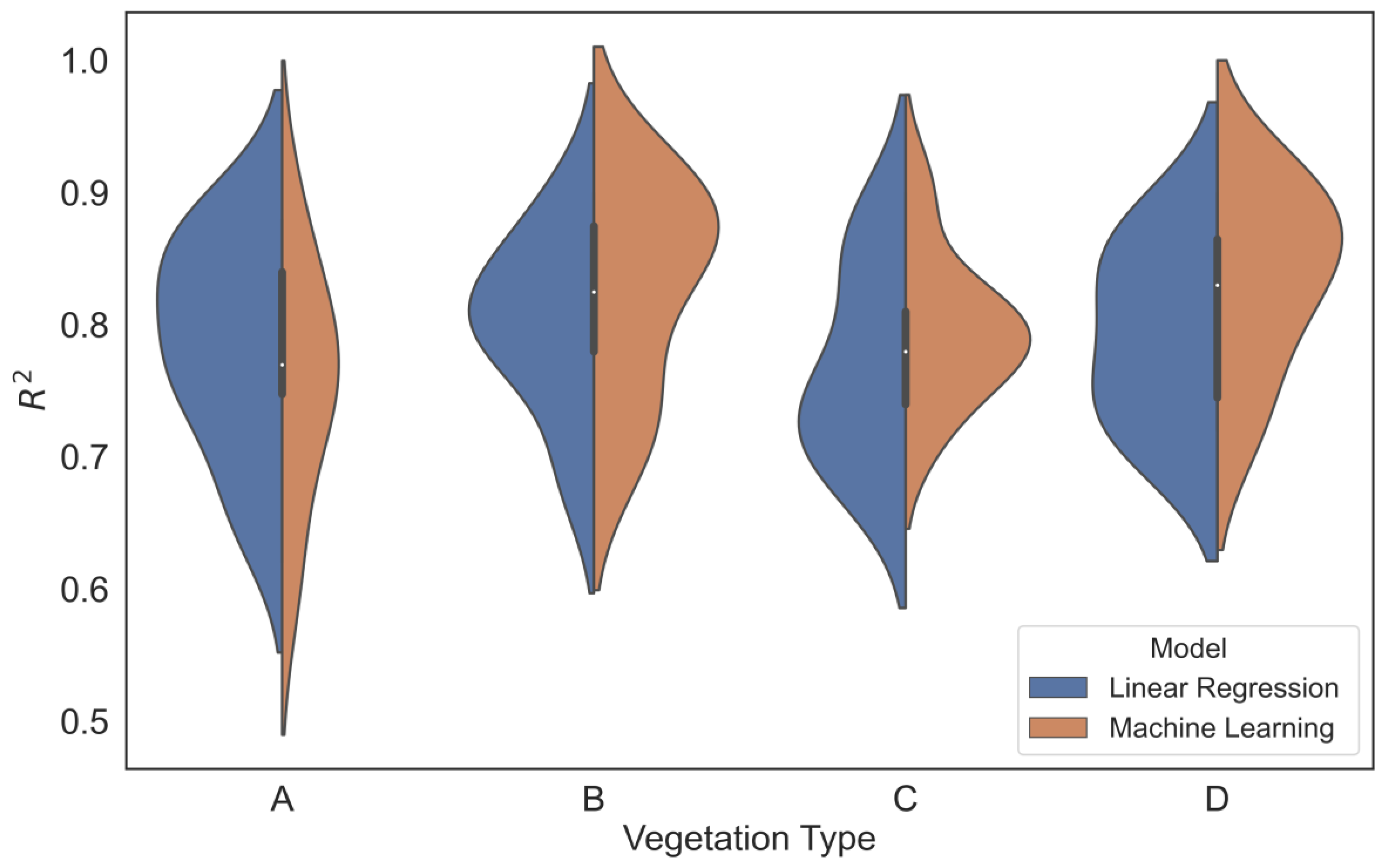
Multiple linear regression (MLR) and random forest (RF) were found to be the most used and most accurate models to estimate the biomass for all vegetation types. The accuracy of biomass estimation models (linear regression and machine learning) was assessed by comparing the range of R2 values across 211 studies (Figure 20). Additionally, a t-test was conducted to examine the statistical significance between two groups of models: linear regression and machine learning, for various vegetation types. In forests, there is no significant difference (p = 0.1615) between the two model types, indicating similar performance. However, for grasses, the p-value (p = 0.0330) signifies a significant difference, emphasizing the importance of machine learning models to estimate the above-ground biomass in grasses. Conversely, for horizontally and vertically growing crops, there is no significant difference (p = 0.2517 and p = 0.1216, respectively), suggesting that both model types perform equally well.
Machine learning (ML) and traditional linear regression models showed similar performance in forests because structural metrics such as tree height and diameter are used to determine biomass, which are easy to obtain and provide strong predictors [236]. The homogenous structure of forests also leads to less complex relationships [237]. ML models outperformed linear regression models for grass biomass estimation due to the complexity and non-linear nature of the data. Grass biomass involves intricate interactions among variables [238]. ML models capture these patterns better. However, ML models showed similar performance to linear regression for estimation of biomass in horizontally and vertically growing crops. This may be due to simpler data relationships and more uniform growth patterns in these crops, where linear regression adequately captures the relationships. The additional complexities addressed by ML models are less impactful in these cases.
Table 7 presents a comprehensive guide for the accurate estimation of AGB using UAS-mounted sensors for different vegetation types, which is based on a thorough review of the literature.

8. Challenges

The main challenges in using UASs for biomass estimation are related to sensors, aircraft platforms, and technical challenges to handle hardware and software.
The spatial resolution of sensors and the signal-to-noise ratio are the main sensor-based challenges that can affect the accuracy of biomass estimates using UASs. High resolution sensors may capture more detailed information but may also be more expensive and require more processing power to analyze the data [178]. A high signal-to-noise ratio can improve the accuracy of estimates but may also increase the cost and complexity of the sensors [183,239]. Careful consideration of cost, accuracy, and complexity is important when selecting sensors for biomass estimation using UASs. Inaccurate estimates may occur if the UAS is not stable, and data are distorted or incomplete. Environmental conditions such as wind and weather can also impact data accuracy by making it difficult for the UAS to maintain stability [22].
Estimating biomass in forests is challenging due to the reflectance mixture and multilevel canopy dossels. Reflectance mixture is when the reflectance of light from a given area is a combination of the reflectance of different species or vegetation present [240]. Multilevel canopy dossels is the presence of multiple canopy layers in a forest. To overcome these challenges, using multiple sensors or different wavelengths of light is recommended. Water, cloud cover, and tidal stage can affect the accuracy of biomass estimation [65]. Cloud cover can affect the accuracy of biomass estimation by reducing the amount of light available to the sensors and causing shadows [90] and other distortions in the data [178]. Dew on the canopies can cause overestimation of vegetation indices [103] and it is recommended to avoid collecting data when dew is present. Vegetation phenology can also affect the correlation between VIs and biomass, and data should be collected during peak biomass and similar seasons [103]. Artifacts in imagery can be a challenge for using UAS images to estimate biomass, but advanced image processing techniques can be used to remove or correct them [65]. Legal restrictions from the Federal Aviation Administration (FAA) can cause gaps and limitations in UAS imagery, making it challenging to detect changes over time. Researchers can minimize the impact by carefully planning the UAS flights [89]. Computing power can be a challenge for UAS images to estimate biomass, requiring significant amount of computing power to process [241,242]. Current battery capacities and flight times can also be a challenge, but researchers may use UASs with larger battery capacities or use multiple batteries to extend flight time [64]. Optical saturation and GPS positional errors can also affect the accuracy of biomass estimation [243]. To address this, researchers may use sensors with a higher dynamic range to avoid optical saturation [45,47]. GPS positional errors can be a significant challenge when using remotely sensed data for biomass estimation, as they can affect the accuracy of the biomass estimates by misaligning the location of the remotely sensed data with the true location of the vegetation, leading to overestimation or underestimation of biomass [242,244].

9. Conclusions

The findings of this study revealed important insights into the use of unmanned aerial systems (UASs) for above-ground biomass (AGB) estimation across different vegetation types. Rotary-wing UASs, particularly quadcopters, were found to be commonly used in agricultural fields, offering specific advantages in terms of their capabilities. Sensor selection varied depending on the vegetation types, with LIDAR and RGB sensors being commonly employed in forests, while RGB, multispectral, and hyperspectral sensors were prevalent in agricultural and grass fields. Regarding flight parameters, the choice of flight altitudes and speeds was influenced by vegetation characteristics and sensor types, with variations observed among different vegetation groups. Additionally, the number of ground control points (GCPs) required for accurate AGB estimation differed based on vegetation type and topographic complexity. To ensure optimal accuracy, data collection during solar noon was preferred, considering factors such as enhanced image quality, solar energy availability, and reduced atmospheric effects. The number of vegetation indices had a significant impact on AGB estimation accuracy in vertically growing crops, whereas its influence was limited in forests, grasses, and horizontally growing crops. Moreover, the choice of plant height metrics varied across vegetation groups, with forests and vertically growing crops relying on the maximum height, while grasses and horizontally growing crops utilized central tendency metrics. In terms of modeling approaches, linear regression, and machine learning models performed similarly in forests, but machine learning models outperformed linear regression models in grasses. However, both modeling approaches yielded comparable results for horizontally and vertically growing crops, indicating their suitability for these vegetation types. The use of UASs for biomass estimation also presented various challenges related to sensors, environmental conditions, reflectance mixture, canopy complexity, water, cloud cover, dew, phenology, image artifacts, legal restrictions, computing power, battery capacity, optical saturation, and GPS errors. Addressing these challenges necessitates careful consideration of sensor selection, timing, advanced image processing techniques, compliance with regulations, and overcoming technical limitations. Overall, our findings provide valuable insights and guidelines for the effective and accurate use of UASs in AGB estimation across different vegetation types. By understanding the specific requirements and characteristics of each vegetation type, researchers and practitioners can make informed decisions regarding platform selection, sensor choice, flight parameters, and modeling approaches, ultimately enhancing the precision and efficiency of biomass estimation using UAS technology.

Author Contributions

Conceptualization, A.B. and P.F.; methodology, A.B. and P.F.; software, A.B.; validation, A.B. and P.F.; formal analysis, A.B.; investigation, A.B. and N.D.; resources, P.F.; data curation, A.B.; writing—original draft preparation, A.B.; writing—review and editing, A.B., N.D., P.G.O., N.B. and P.F.; visualization, A.B.; supervision, P.F.; project administration, P.F.; funding acquisition, P.F. All authors have read and agreed to the published version of the manuscript.

Funding

This review paper was supported by funding from the North Dakota Agricultural Experiment Station, project number FARG080021.

Data Availability Statement

The data used in this research are available upon request to the corresponding author.

Conflicts of Interest

The authors declare no conflict of interest.

References

  1. Wilkes, P.; Disney, M.; Vicari, M.B.; Calders, K.; Burt, A. Estimating Urban above Ground Biomass with Multi-Scale LiDAR. Carbon Balance Manag. 2018, 13, 10. [Google Scholar] [CrossRef]
  2. Poley, L.G.; McDermid, G.J. A Systematic Review of the Factors Influencing the Estimation of Vegetation Aboveground Biomass Using Unmanned Aerial Systems. Remote Sens. 2020, 12, 1052. [Google Scholar] [CrossRef] [Green Version]
  3. Liu, K.; Shen, X.; Cao, L.; Wang, G.; Cao, F. The Evaluation of Parametric and Non-Parametric Models for Total Forest Biomass Estimation Using UAS-LiDAR. In Proceedings of the 5th International Workshop on Earth Observation and Remote Sensing Applications, EORSA 2018—Proceedings, Xi’an, China, 18–20 June 2018. [Google Scholar]
  4. Yue, J.; Zhou, C.; Guo, W.; Feng, H.; Xu, K. Estimation of Winter-Wheat above-Ground Biomass Using the Wavelet Analysis of Unmanned Aerial Vehicle-Based Digital Images and Hyperspectral Crop Canopy Images. Int. J. Remote Sens. 2021, 42, 1602–1622. [Google Scholar] [CrossRef]
  5. Duncanson, L.; Armston, J.; Disney, M.; Avitabile, V.; Barbier, N.; Calders, K.; Carter, S.; Chave, J.; Herold, M.; Crowther, T.W.; et al. The Importance of Consistent Global Forest Aboveground Biomass Product Validation. Surv. Geophys. 2019, 40, 979–999. [Google Scholar] [CrossRef] [Green Version]
  6. Wan, X.; Li, Z.; Chen, E.; Zhao, L.; Zhang, W.; Xu, K. Forest Aboveground Biomass Estimation Using Multi-Features Extracted by Fitting Vertical Backscattered Power Profile of Tomographic Sar. Remote Sens. 2021, 13, 186. [Google Scholar] [CrossRef]
  7. Moradi, F.; Mohammad, S.; Sadeghi, M.; Heidarlou, H.B. Above-Ground Biomass Estimation in a Mediterranean Sparse Coppice Oak Forest Using Sentinel-2 Data. Ann. For. Res. 2022, 65, 165–182. [Google Scholar] [CrossRef]
  8. Khan, I.A.; Khan, W.R.; Ali, A.; Nazre, M. Assessment of Above-Ground Biomass in Pakistan Forest Ecosystem’s Carbon Pool: A Review. Forests 2021, 12, 586. [Google Scholar] [CrossRef]
  9. Chang, G.J.; Oh, Y.; Goldshleger, N.; Shoshany, M. Biomass Estimation of Crops and Natural Shrubs by Combining Red-Edge Ratio with Normalized Difference Vegetation Index. J. Appl. Remote Sens. 2022, 16, 14501. [Google Scholar] [CrossRef]
  10. Xu, C.; Ding, Y.; Zheng, X.; Wang, Y.; Zhang, R.; Zhang, H.; Dai, Z. A Comprehensive Comparison of Machine Learning and Feature Selection Methods for Maize Biomass Estimation Using Sentinel-1 SAR, Sentinel-2 Vegetation Indices, and Biophysical Variables. Remote Sens. 2022, 14, 4083. [Google Scholar] [CrossRef]
  11. Ballesteros, R.; Ortega, J.F.; Hernandez, D.; Moreno, M.A. Onion Biomass Monitoring Using UAV-Based RGB Imaging. Precis. Agric. 2018, 19, 840–857. [Google Scholar] [CrossRef]
  12. Alebele, Y.; Zhang, X.; Wang, W.; Yang, G.; Yao, X.; Zheng, H.; Zhu, Y.; Cao, W.; Cheng, T. Estimation of Canopy Biomass Components in Paddy Rice from Combined Optical and SAR Data Using Multi-Target Gaussian Regressor Stacking. Remote Sens. 2020, 12, 2564. [Google Scholar] [CrossRef]
  13. Liu, Y.; Feng, H.; Yue, J.; Jin, X.; Li, Z.; Yang, G. Estimation of Potato Above-Ground Biomass Based on Unmanned Aerial Vehicle Red-Green-Blue Images with Different Texture Features and Crop Height. Front. Plant Sci. 2022, 13, 938216. [Google Scholar] [CrossRef] [PubMed]
  14. Vargas, J.J.Q.; Zhang, C.; Smitchger, J.A.; McGee, R.J.; Sankaran, S. Phenotyping of Plant Biomass and Performance Traits Using Remote Sensing Techniques in Pea (Pisum sativum, L.). Sensors 2019, 19, 2031. [Google Scholar] [CrossRef] [PubMed] [Green Version]
  15. Acorsi, M.G.; das Dores Abati Miranda, F.; Martello, M.; Smaniotto, D.A.; Sartor, L.R. Estimating Biomass of Black Oat Using UAV-Based RGB Imaging. Agronomy 2019, 9, 344. [Google Scholar] [CrossRef] [Green Version]
  16. Bar-On, Y.M.; Phillips, R.; Milo, R. The Biomass Distribution on Earth. Proc. Natl. Acad. Sci. USA 2018, 115, 6506–6511. [Google Scholar] [CrossRef] [PubMed] [Green Version]
  17. Zhang, H.; Sun, Y.; Chang, L.; Qin, Y.; Chen, J.; Qin, Y.; Du, J.; Yi, S.; Wang, Y. Estimation of Grassland Canopy Height and Aboveground Biomass at the Quadrat Scale Using Unmanned Aerial Vehicle. Remote Sens. 2018, 10, 851. [Google Scholar] [CrossRef] [Green Version]
  18. Wang, Z.; Ma, Y.; Zhang, Y.; Shang, J. Review of Remote Sensing Applications in Grassland Monitoring. Remote Sens. 2022, 14, 2903. [Google Scholar] [CrossRef]
  19. Clementini, C.; Pomente, A.; Latini, D.; Kanamaru, H.; Vuolo, M.R.; Heureux, A.; Fujisawa, M.; Schiavon, G.; Del Frate, F. Long-Term Grass Biomass Estimation of Pastures from Satellite Data. Remote Sens. 2020, 12, 2160. [Google Scholar] [CrossRef]
  20. Muumbe, T.P.; Baade, J.; Singh, J.; Schmullius, C.; Thau, C. Terrestrial Laser Scanning for Vegetation Analyses with a Special Focus on Savannas. Remote Sens. 2021, 13, 507. [Google Scholar] [CrossRef]
  21. Grybas, H.; Congalton, R.G. Evaluating the Impacts of Flying Height and Forward Overlap on Tree Height Estimates Using Unmanned Aerial Systems. Forests 2022, 13, 1462. [Google Scholar] [CrossRef]
  22. Delavarpour, N.; Koparan, C.; Nowatzki, J.; Bajwa, S.; Sun, X. A Technical Study on UAV Characteristics for Precision Agriculture Applications and Associated Practical Challenges. Remote Sens. 2021, 13, 1204. [Google Scholar] [CrossRef]
  23. Gil-Docampo, M.L.; Arza-García, M.; Ortiz-Sanz, J.; Martínez-Rodríguez, S.; Marcos-Robles, J.L.; Sánchez-Sastre, L.F. Above-Ground Biomass Estimation of Arable Crops Using UAV-Based SfM Photogrammetry. Geocarto Int. 2020, 35, 687–699. [Google Scholar] [CrossRef]
  24. Wan, L.; Zhang, J.; Dong, X.; Du, X.; Zhu, J.; Sun, D.; Liu, Y.; He, Y.; Cen, H. Unmanned Aerial Vehicle-Based Field Phenotyping of Crop Biomass Using Growth Traits Retrieved from PROSAIL Model. Comput. Electron. Agric. 2021, 187, 106304. [Google Scholar] [CrossRef]
  25. Li, D.; Gu, X.; Pang, Y.; Chen, B.; Liu, L. Estimation of Forest Aboveground Biomass and Leaf Area Index Based on Digital Aerial Photograph Data in Northeast China. Forests 2018, 9, 275. [Google Scholar] [CrossRef] [Green Version]
  26. Zhao, Y.; Liu, X.; Wang, Y.; Zheng, Z.; Zheng, S.; Zhao, D.; Bai, Y. UAV-Based Individual Shrub Aboveground Biomass Estimation Calibrated against Terrestrial LiDAR in a Shrub-Encroached Grassland. Int. J. Appl. Earth Obs. Geoinf. 2021, 101, 102358. [Google Scholar] [CrossRef]
  27. Gano, B.; Dembele, J.S.B.; Ndour, A.; Luquet, D.; Beurier, G.; Diouf, D.; Audebert, A. Using Uav Borne, Multi-Spectral Imaging for the Field Phenotyping of Shoot Biomass, Leaf Area Index and Height of West African Sorghum Varieties under Two Contrasted Water Conditions. Agronomy 2021, 11, 850. [Google Scholar] [CrossRef]
  28. Jiang, F.; Kutia, M.; Ma, K.; Chen, S.; Long, J.; Sun, H. Estimating the Aboveground Biomass of Coniferous Forest in Northeast China Using Spectral Variables, Land Surface Temperature and Soil Moisture. Sci. Total Environ. 2021, 785, 147335. [Google Scholar] [CrossRef] [PubMed]
  29. Zhao, Q.; Yu, S.; Zhao, F.; Tian, L.; Zhao, Z. Comparison of Machine Learning Algorithms for Forest Parameter Estimations and Application for Forest Quality Assessments. For. Ecol. Manag. 2019, 434, 224–234. [Google Scholar] [CrossRef]
  30. Jin, S.; Su, Y.; Song, S.; Xu, K.; Hu, T.; Yang, Q.; Wu, F.; Xu, G.; Ma, Q.; Guan, H.; et al. Non-Destructive Estimation of Field Maize Biomass Using Terrestrial Lidar: An Evaluation from Plot Level to Individual Leaf Level. Plant Methods 2020, 16, 69. [Google Scholar] [CrossRef]
  31. Li, B.; Xu, X.; Zhang, L.; Han, J.; Bian, C.; Li, G.; Liu, J.; Jin, L. Above-Ground Biomass Estimation and Yield Prediction in Potato by Using UAV-Based RGB and Hyperspectral Imaging. ISPRS J. Photogramm. Remote Sens. 2020, 162, 161–172. [Google Scholar] [CrossRef]
  32. Grüner, E.; Astor, T.; Wachendorf, M. Biomass Prediction of Heterogeneous Temperate Grasslands Using an SFM Approach Based on UAV Imaging. Agronomy 2019, 9, 54. [Google Scholar] [CrossRef] [Green Version]
  33. de Almeida, C.T.; Galvão, L.S.; de Oliveira Cruz e Aragão, L.E.; Ometto, J.P.H.B.; Jacon, A.D.; de Souza Pereira, F.R.; Sato, L.Y.; Lopes, A.P.; de Alencastro Graça, P.M.L.; de Jesus Silva, C.V.; et al. Combining LiDAR and Hyperspectral Data for Aboveground Biomass Modeling in the Brazilian Amazon Using Different Regression Algorithms. Remote Sens. Environ. 2019, 232, 111323. [Google Scholar] [CrossRef]
  34. Adeluyi, O.; Harris, A.; Foster, T.; Clay, G.D. Exploiting Centimetre Resolution of Drone-Mounted Sensors for Estimating Mid-Late Season above Ground Biomass in Rice. Eur. J. Agron. 2022, 132, 126411. [Google Scholar] [CrossRef]
  35. Swayze, N.C.; Tinkham, W.T.; Creasy, M.B.; Vogeler, J.C.; Hoffman, C.M.; Hudak, A.T. Influence of UAS Flight Altitude and Speed on Aboveground Biomass Prediction. Remote Sens. 2022, 14, 1989. [Google Scholar] [CrossRef]
  36. Salum, R.B.; Souza-Filho, P.W.M.; Simard, M.; Silva, C.A.; Fernandes, M.E.B.; Cougo, M.F.; do Nascimento, W.; Rogers, K. Improving Mangrove Above-Ground Biomass Estimates Using LiDAR. Estuar. Coast. Shelf Sci. 2020, 236, 106585. [Google Scholar] [CrossRef]
  37. Domingo, D.; Ørka, H.O.; Næsset, E.; Kachamba, D.; Gobakken, T. Effects of UAV Image Resolution, Camera Type, and Image Overlap on Accuracy of Biomass Predictions in a Tropical Woodland. Remote Sens. 2019, 11, 948. [Google Scholar] [CrossRef] [Green Version]
  38. Viljanen, N.; Honkavaara, E.; Näsi, R.; Hakala, T.; Niemeläinen, O.; Kaivosoja, J. A Novel Machine Learning Method for Estimating Biomass of Grass Swards Using a Photogrammetric Canopy Height Model, Images and Vegetation Indices Captured by a Drone. Agriculture 2018, 8, 70. [Google Scholar] [CrossRef] [Green Version]
  39. Swayze, N.C.; Tinkham, W.T.; Vogeler, J.C.; Hudak, A.T. Influence of Flight Parameters on UAS-Based Monitoring of Tree Height, Diameter, and Density. Remote Sens. Environ. 2021, 263, 112540. [Google Scholar] [CrossRef]
  40. Ye, N.; van Leeuwen, L.; Nyktas, P. Analysing the Potential of UAV Point Cloud as Input in Quantitative Structure Modelling for Assessment of Woody Biomass of Single Trees. Int. J. Appl. Earth Obs. Geoinf. 2019, 81, 47–57. [Google Scholar] [CrossRef]
  41. Zhang, H.; Wang, C.; Zhu, J.; Fu, H.; Xie, Q.; Shen, P. Forest Above-Ground Biomass Estimation Using Single-Baseline Polarization Coherence Tomography with P-Band PolInSAR Data. Forests 2018, 9, 163. [Google Scholar] [CrossRef] [Green Version]
  42. Näsi, R.; Viljanen, N.; Kaivosoja, J.; Alhonoja, K.; Hakala, T.; Markelin, L.; Honkavaara, E. Estimating Biomass and Nitrogen Amount of Barley and Grass Using UAV and Aircraft Based Spectral and Photogrammetric 3D Features. Remote Sens. 2018, 10, 1082. [Google Scholar] [CrossRef] [Green Version]
  43. d’Oliveira, M.V.N.; Broadbent, E.N.; Oliveira, L.C.; Almeida, D.R.A.; Papa, D.A.; Ferreira, M.E.; Zambrano, A.M.A.; Silva, C.A.; Avino, F.S.; Prata, G.A.; et al. Aboveground Biomass Estimation in Amazonian Tropical Forests: A Comparison of Aircraft- and GatorEye UAV-Borne LiDAR Data in the Chico Mendes Extractive Reserve in Acre, Brazil. Remote Sens. 2020, 12, 1754. [Google Scholar] [CrossRef]
  44. Guascal, E.; Rojas, S.; Kirby, E.; Toulkeridis, T.; Fuertes, W.; Heredia, M. Application of Remote Sensing Techniques in the Estimation of Forest Biomass of a Recreation Area by UAV and RADAR Images in Ecuador. In Proceedings of the 2020 Seventh International Conference on eDemocracy & eGovernment (ICEDEG), Buenos Aires, Argentina, 22–24 April 2020; pp. 183–190. [Google Scholar]
  45. Jiang, Q.; Fang, S.; Peng, Y.; Gong, Y.; Zhu, R.; Wu, X.; Ma, Y.; Duan, B.; Liu, J. UAV-Based Biomass Estimation for Rice-Combining Spectral, TIN-Based Structural and Meteorological Features. Remote Sens. 2019, 11, 890. [Google Scholar] [CrossRef] [Green Version]
  46. Cao, L.; Liu, K.; Shen, X.; Wu, X.; Liu, H. Estimation of Forest Structural Parameters Using UAV-LiDAR Data and a Process-Based Model in Ginkgo Planted Forests. IEEE J. Sel. Top. Appl. Earth Obs. Remote Sens. 2019, 12, 4175–4190. [Google Scholar] [CrossRef]
  47. Niu, Y.; Zhang, L.; Zhang, H.; Han, W.; Peng, X. Estimating Above-Ground Biomass of Maize Using Features Derived from UAV-Based RGB Imagery. Remote Sens. 2019, 11, 1261. [Google Scholar] [CrossRef] [Green Version]
  48. Zhu, W.; Sun, Z.; Peng, J.; Huang, Y.; Li, J.; Zhang, J.; Yang, B.; Liao, X. Estimating Maize Above-Ground Biomass Using 3D Point Clouds of Multi-Source Unmanned Aerial Vehicle Data at Multi-Spatial Scales. Remote Sens. 2019, 11, 2678. [Google Scholar] [CrossRef] [Green Version]
  49. Liu, K.; Shen, X.; Cao, L.; Wang, G.; Cao, F. Estimating Forest Structural Attributes Using UAV-LiDAR Data in Ginkgo Plantations. ISPRS J. Photogramm. Remote Sens. 2018, 146, 465–482. [Google Scholar] [CrossRef]
  50. Ku, N.W.; Popescu, S.C. A Comparison of Multiple Methods for Mapping Local-Scale Mesquite Tree Aboveground Biomass with Remotely Sensed Data. Biomass Bioenergy 2019, 122, 270–279. [Google Scholar] [CrossRef]
  51. Dorado-Roda, I.; Pascual, A.; Godinho, S.; Silva, C.A.; Botequim, B.; Rodríguez-Gonzálvez, P.; González-Ferreiro, E.; Guerra-Hernández, J. Assessing the Accuracy of Gedi Data for Canopy Height and Aboveground Biomass Estimates in Mediterranean Forests. Remote Sens. 2021, 13, 2279. [Google Scholar] [CrossRef]
  52. Navarro, A.; Young, M.; Allan, B.; Carnell, P.; Macreadie, P.; Ierodiaconou, D. The Application of Unmanned Aerial Vehicles (UAVs) to Estimate above-Ground Biomass of Mangrove Ecosystems. Remote Sens. Environ. 2020, 242, 111747. [Google Scholar] [CrossRef]
  53. Zheng, L.; Tao, J.; Bao, Q.; Weng, S.; Zhang, Y.; Zhao, J.; Huang, L. Combining Spectral and Textures of Digital Imagery for Wheat Aboveground Biomass Estimation. In Proceedings of the International Conference on Electronic Information Technology (EIT 2022), Chengdu, China, 23 May 2022; Volume 12254, p. 1225419. [Google Scholar] [CrossRef]
  54. Herwitz, S.; Johnson, L.; Arvesen, J.; Higgins, R.; Leung, J.; Dunagan, S. Precision Agriculture as a Commercial Application for Solar-Powered Unmanned Aerial Vehicles. In Proceedings of the 1st UAV Conference, Infotech@Aerospace Conferences, Portsmouth, VA, USA, 20–23 May 2002. [Google Scholar] [CrossRef]
  55. Wang, T.; Liu, Y.; Wang, M.; Fan, Q.; Tian, H.; Qiao, X.; Li, Y. Applications of UAS in Crop Biomass Monitoring: A Review. Front. Plant Sci. 2021, 12, 616689. [Google Scholar] [CrossRef]
  56. Chao, Z.; Liu, N.; Zhang, P.; Ying, T.; Song, K. Estimation Methods Developing with Remote Sensing Information for Energy Crop Biomass: A Comparative Review. Biomass Bioenergy 2019, 122, 414–425. [Google Scholar] [CrossRef]
  57. Panday, U.S.; Pratihast, A.K.; Aryal, J.; Kayastha, R.B. A Review on Drone-Based Data Solutions for Cereal Crops. Drones 2020, 4, 41. [Google Scholar] [CrossRef]
  58. Olson, D.; Anderson, J. Review on Unmanned Aerial Vehicles, Remote Sensors, Imagery Processing, and Their Applications in Agriculture. Agron. J. 2021, 113, 971–992. [Google Scholar] [CrossRef]
  59. Xie, C.; Yang, C. A Review on Plant High-Throughput Phenotyping Traits Using UAV-Based Sensors. Comput. Electron. Agric. 2020, 178, 105731. [Google Scholar] [CrossRef]
  60. Feng, L.; Chen, S.; Zhang, C.; Zhang, Y.; He, Y. A Comprehensive Review on Recent Applications of Unmanned Aerial Vehicle Remote Sensing with Various Sensors for High-Throughput Plant Phenotyping. Comput. Electron. Agric. 2021, 182, 106033. [Google Scholar] [CrossRef]
  61. Dat Pham, T.; Xia, J.; Thang Ha, N.; Tien Bui, D.; Nhu Le, N.; Tekeuchi, W. A Review of Remote Sensing Approaches for Monitoring Blue Carbon Ecosystems: Mangroves, Sea Grasses and Salt Marshes during 2010–2018. Sensors 2019, 19, 1933. [Google Scholar] [CrossRef] [Green Version]
  62. Goodbody, T.R.H.; Coops, N.C.; White, J.C. Digital Aerial Photogrammetry for Updating Area-Based Forest Inventories: A Review of Opportunities, Challenges, and Future Directions. Curr. For. Rep. 2019, 5, 55–75. [Google Scholar] [CrossRef] [Green Version]
  63. Armi, L.; Fekri-Ershad, S. Texture Image Analysis and Texture Classification Methods—A Review. arXiv 2019, arXiv:1904.06554. [Google Scholar]
  64. Mohsan, S.A.H.; Khan, M.A.; Noor, F.; Ullah, I.; Alsharif, M.H. Towards the Unmanned Aerial Vehicles (UAVs): A Comprehensive Review. Drones 2022, 6, 147. [Google Scholar] [CrossRef]
  65. Morgan, G.R.; Hodgson, M.E.; Wang, C.; Schill, S.R. Unmanned Aerial Remote Sensing of Coastal Vegetation: A Review. Ann. GIS 2022, 28, 385–399. [Google Scholar] [CrossRef]
  66. Ji, G.; Shi, C.; Xue, M. The Application of Unmanned Aerial Vehicles Data Communication in Agriculture. In Proceedings of the 2022 IEEE Conference on Telecommunications, Optics and Computer Science (TOCS), Dalian, China, 11–12 December 2022; pp. 1378–1382. [Google Scholar]
  67. Jońca, J.; Pawnuk, M.; Bezyk, Y.; Arsen, A.; Sówka, I. Drone-Assisted Monitoring of Atmospheric Pollution—A Comprehensive Review. Sustainability 2022, 14, 11516. [Google Scholar] [CrossRef]
  68. Yu, Y.; Pan, Y.; Yang, X.; Fan, W. Spatial Scale Effect and Correction of Forest Aboveground Biomass Estimation Using Remote Sensing. Remote Sens. 2022, 14, 2828. [Google Scholar] [CrossRef]
  69. Ferdaus, M.M.; Anavatti, S.G.; Pratama, M.; Garratt, M.A. Towards the Use of Fuzzy Logic Systems in Rotary Wing Unmanned Aerial Vehicle: A Review. Artif. Intell. Rev. 2020, 53, 257–290. [Google Scholar] [CrossRef]
  70. Freitas Moreira, F.; Rojas de Oliveira, H.; Lopez, M.A.; Abughali, B.J.; Gomes, G.; Cherkauer, K.A.; Brito, L.F.; Rainey, K.M. High-Throughput Phenotyping and Random Regression Models Reveal Temporal Genetic Control of Soybean Biomass Production. Front. Plant Sci. 2021, 12, 715983. [Google Scholar] [CrossRef]
  71. Holzhauser, K.; Räbiger, T.; Rose, T.; Kage, H.; Kühling, I. Estimation of Biomass and N Uptake in Different Winter Cover Crops from UAV-Based Multispectral Canopy Reflectance Data. Remote Sens. 2022, 14, 4525. [Google Scholar] [CrossRef]
  72. Schucknecht, A.; Seo, B.; Krämer, A.; Asam, S.; Atzberger, C.; Kiese, R. Estimating Dry Biomass and Plant Nitrogen Concentration in Pre-Alpine Grasslands with Low-Cost UAS-Borne Multispectral Data—A Comparison of Sensors, Algorithms, and Predictor Sets. Biogeosciences 2022, 19, 2699–2727. [Google Scholar] [CrossRef]
  73. Zhang, Y.; Xia, C.; Zhang, X.; Cheng, X.; Feng, G.; Wang, Y.; Gao, Q. Estimating the Maize Biomass by Crop Height and Narrowband Vegetation Indices Derived from UAV-Based Hyperspectral Images. Ecol. Indic. 2021, 129, 107985. [Google Scholar] [CrossRef]
  74. Grüner, E.; Wachendorf, M.; Astor, T. The Potential of UAV-Borne Spectral and Textural Information for Predicting Aboveground Biomass and N Fixation in Legume-Grass Mixtures. PLoS ONE 2020, 15, e0234703. [Google Scholar] [CrossRef]
  75. Choudhury, M.R.; Das, S.; Christopher, J.; Apan, A.; Chapman, S.; Menzies, N.W.; Dang, Y.P. Improving Biomass and Grain Yield Prediction of Wheat Genotypes on Sodic Soil Using Integrated High-Resolution Multispectral, Hyperspectral, 3d Point Cloud, and Machine Learning Techniques. Remote Sens. 2021, 13, 3482. [Google Scholar] [CrossRef]
  76. Ren, H.; Xiao, W.; Zhao, Y.; Hu, Z. Land Damage Assessment Using Maize Aboveground Biomass Estimated from Unmanned Aerial Vehicle in High Groundwater Level Regions Affected by Underground Coal Mining. Environ. Sci. Pollut. Res. 2020, 27, 21666–21679. [Google Scholar] [CrossRef]
  77. Li, J.; Shi, Y.; Veeranampalayam-Sivakumar, A.N.; Schachtman, D.P. Elucidating Sorghum Biomass, Nitrogen and Chlorophyll Contents with Spectral and Morphological Traits Derived from Unmanned Aircraft System. Front. Plant Sci. 2018, 9, 1406. [Google Scholar] [CrossRef]
  78. Li, Z.; Zhao, Y.; Taylor, J.; Gaulton, R.; Jin, X.; Song, X.; Li, Z.; Meng, Y.; Chen, P.; Feng, H.; et al. Comparison and Transferability of Thermal, Temporal and Phenological-Based in-Season Predictions of above-Ground Biomass in Wheat Crops from Proximal Crop Reflectance Data. Remote Sens. Environ. 2022, 273, 112967. [Google Scholar] [CrossRef]
  79. Barnetson, J.; Phinn, S.; Scarth, P. Estimating Plant Pasture Biomass and Quality from UAV Imaging across Queensland’s Rangelands. AgriEngineering 2020, 2, 35. [Google Scholar] [CrossRef]
  80. Galán, R.J.; Bernal-Vasquez, A.-M.; Jebsen, C.; Piepho, H.-P.; Thorwarth, P.; Steffan, P.; Gordillo, A.; Miedaner, T. Integration of Genotypic, Hyperspectral, and Phenotypic Data to Improve Biomass Yield Prediction in Hybrid Rye. Theor. Appl. Genet. 2020, 133, 3001–3015. [Google Scholar] [CrossRef]
  81. Bates, J.; Jonard, F.; Bajracharya, R.; Vereecken, H.; Montzka, C. Machine Learning with UAS LiDAR for Winter Wheat Biomass Estimations. AGILE GIScience Ser. 2022, 3, 23. [Google Scholar] [CrossRef]
  82. Bates, J.S.; Montzka, C.; Schmidt, M.; Jonard, F. Estimating Canopy Density Parameters Time-Series for Winter Wheat Using Uas Mounted Lidar. Remote Sens. 2021, 13, 710. [Google Scholar] [CrossRef]
  83. Zhang, X.; Bao, Y.; Wang, D.; Xin, X.; Ding, L.; Xu, D.; Hou, L.; Shen, J. Using UAV LiDAR to Extract Vegetation Parameters of Inner Mongolian Grassland. Remote Sens. 2021, 13, 656. [Google Scholar] [CrossRef]
  84. Chavez, J.L.; Torres-Rua, A.F.; Woldt, W.E.; Zhang, H.; Robertson, C.C.; Marek, G.W.; Wang, D.; Heeren, D.M.; Taghvaeian, S.; Neale, C.M.; et al. A Decade of Unmanned Aerial Systems in Irrigated Agriculture in the Western US. Appl. Eng. Agric. 2020, 36, 423–436. [Google Scholar] [CrossRef]
  85. Turton, A.E.; Augustin, N.H.; Mitchard, E.T.A. Improving Estimates and Change Detection of Forest Above-Ground Biomass Using Statistical Methods. Remote Sens. 2022, 14, 4911. [Google Scholar] [CrossRef]
  86. Kaimaris, D.; Kandylas, A. Small Multispectral UAV Sensor and Its Image Fusion Capability in Cultural Heritage Applications. Heritage 2020, 3, 1046–1062. [Google Scholar] [CrossRef]
  87. Maesano, M.; Khoury, S.; Nakhle, F.; Firrincieli, A.; Gay, A.; Tauro, F.; Harfouche, A. UAV-Based LiDAR for High-Throughput Determination of Plant Height and Above-Ground Biomass of the Bioenergy Grass Arundo Donax. Remote Sens. 2020, 12, 3464. [Google Scholar] [CrossRef]
  88. Zhang, L.; Shao, Z.; Liu, J.; Cheng, Q. Deep Learning Based Retrieval of Forest Aboveground Biomass from Combined LiDAR and Landsat 8 Data. Remote Sens. 2019, 11, 1459. [Google Scholar] [CrossRef] [Green Version]
  89. Durgan, S.D.; Zhang, C.; Duecaster, A.; Fourney, F.; Su, H. Unmanned Aircraft System Photogrammetry for Mapping Diverse Vegetation Species in a Heterogeneous Coastal Wetland. Wetlands 2020, 40, 2621–2633. [Google Scholar] [CrossRef]
  90. Rupasinghe, P.A.; Simic Milas, A.; Arend, K.; Simonson, M.A.; Mayer, C.; Mackey, S. Classification of Shoreline Vegetation in the Western Basin of Lake Erie Using Airborne Hyperspectral Imager HSI2, Pleiades and UAV Data. Int. J. Remote Sens. 2019, 40, 3008–3028. [Google Scholar] [CrossRef]
  91. Borra-Serrano, I.; De Swaef, T.; Muylle, H.; Nuyttens, D.; Vangeyte, J.; Mertens, K.; Saeys, W.; Somers, B.; Roldán-Ruiz, I.; Lootens, P. Canopy Height Measurements and Non-Destructive Biomass Estimation of Lolium Perenne Swards Using UAV Imagery. Grass Forage Sci. 2019, 74, 356–369. [Google Scholar] [CrossRef]
  92. Holiaka, D.; Kato, H.; Yoschenko, V.; Onda, Y.; Igarashi, Y.; Nanba, K.; Diachuk, P.; Holiaka, M.; Zadorozhniuk, R.; Kashparov, V.; et al. Scots Pine Stands Biomass Assessment Using 3D Data from Unmanned Aerial Vehicle Imagery in the Chernobyl Exclusion Zone. J. Environ. Manag. 2021, 295, 113319. [Google Scholar] [CrossRef]
  93. de Alckmin, G.T.; Kooistra, L.; Rawnsley, R.; de Bruin, S.; Lucieer, A. Retrieval of Hyperspectral Information from Multispectral Data for Perennial Ryegrass Biomass Estimation. Sensors 2020, 20, 7192. [Google Scholar] [CrossRef]
  94. Yue, J.; Feng, H.; Jin, X.; Yuan, H.; Li, Z.; Zhou, C.; Yang, G.; Tian, Q. A Comparison of Crop Parameters Estimation Using Images from UAV-Mounted Snapshot Hyperspectral Sensor and High-Definition Digital Camera. Remote Sens. 2018, 10, 1138. [Google Scholar] [CrossRef] [Green Version]
  95. Schulze-Brüninghoff, D.; Hensgen, F.; Wachendorf, M.; Astor, T. Methods for LiDAR-Based Estimation of Extensive Grassland Biomass. Comput. Electron. Agric. 2019, 156, 693–699. [Google Scholar] [CrossRef]
  96. Guo, Q.; Wu, F.; Pang, S.; Zhao, X.; Chen, L.; Liu, J.; Xue, B.; Xu, G.; Li, L.; Jing, H.; et al. Crop 3D—A LiDAR Based Platform for 3D High-Throughput Crop Phenotyping. Sci. China Life Sci. 2018, 61, 328–339. [Google Scholar] [CrossRef] [PubMed]
  97. David, R.M.; Rosser, N.J.; Donoghue, D.N. Improving above Ground Biomass Estimates of Southern Africa Dryland Forests by Combining Sentinel-1 SAR and Sentinel-2 Multispectral Imagery. Remote Sens. Environ. 2022, 282, 113232. [Google Scholar] [CrossRef]
  98. Chen, L.; Ren, C.; Bao, G.; Zhang, B.; Wang, Z.; Liu, M.; Man, W.; Liu, J. Improved Object-Based Estimation of Forest Aboveground Biomass by Integrating LiDAR Data from GEDI and ICESat-2 with Multi-Sensor Images in a Heterogeneous Mountainous Region. Remote Sens. 2022, 14, 2743. [Google Scholar] [CrossRef]
  99. Änäkkälä, M.; Lajunen, A.; Hakojärvi, M.; Alakukku, L. Evaluation of the Influence of Field Conditions on Aerial Multispectral Images and Vegetation Indices. Remote Sens. 2022, 14, 4792. [Google Scholar] [CrossRef]
  100. Lussem, U.; Schellberg, J.; Bareth, G. Monitoring Forage Mass with Low-Cost UAV Data: Case Study at the Rengen Grassland Experiment. PFG—J. Photogramm. Remote Sens. Geoinf. Sci. 2020, 88, 407–422. [Google Scholar] [CrossRef]
  101. Halme, E.; Pellikka, P.; Mõttus, M. Utility of Hyperspectral Compared to Multispectral Remote Sensing Data in Estimating Forest Biomass and Structure Variables in Finnish Boreal Forest. Int. J. Appl. Earth Obs. Geoinf. 2019, 83, 101942. [Google Scholar] [CrossRef]
  102. Sharma, P.; Leigh, L.; Chang, J.; Maimaitijiang, M.; Caffé, M. Above-Ground Biomass Estimation in Oats Using UAV Remote Sensing and Machine Learning. Sensors 2022, 22, 601. [Google Scholar] [CrossRef]
  103. Jayathunga, S.; Owari, T.; Tsuyuki, S. Digital Aerial Photogrammetry for Uneven-Aged Forest Management: Assessing the Potential to Reconstruct Canopy Structure and Estimate Living Biomass. Remote Sens. 2019, 11, 338. [Google Scholar] [CrossRef] [Green Version]
  104. Jaskierniak, D.; Lucieer, A.; Kuczera, G.; Turner, D.; Lane, P.; Benyon, R.; Haydon, S. Individual Tree Detection and Crown Delineation from Unmanned Aircraft System (UAS) LiDAR in Structurally Complex Mixed Species Eucalypt Forests. ISPRS J. Photogramm. Remote Sens. 2021, 171, 171–187. [Google Scholar] [CrossRef]
  105. Singh, K.K.; Frazier, A.E. A Meta-Analysis and Review of Unmanned Aircraft System (UAS) Imagery for Terrestrial Applications. Int. J. Remote Sens. 2018, 39, 5078–5098. [Google Scholar] [CrossRef]
  106. Han, L.; Yang, G.; Dai, H.; Xu, B.; Yang, H.; Feng, H.; Li, Z.; Yang, X. Modeling Maize Above-Ground Biomass Based on Machine Learning Approaches Using UAV Remote-Sensing Data. Plant Methods 2019, 15, 10. [Google Scholar] [CrossRef] [PubMed] [Green Version]
  107. Pang, H.; Zhang, A.; Kang, X.; He, N.; Dong, G. Estimation of the Grassland Aboveground Biomass of the Inner Mongolia Plateau Using the Simulated Spectra of Sentinel-2 Images. Remote Sens. 2020, 12, 4155. [Google Scholar] [CrossRef]
  108. Royo, S.; Ballesta-Garcia, M. An Overview of Lidar Imaging Systems for Autonomous Vehicles. Appl. Sci. 2019, 9, 4093. [Google Scholar] [CrossRef] [Green Version]
  109. Zhang, C.; Ang, M.H.; Rus, D. Robust Lidar Localization for Autonomous Driving in Rain. In Proceedings of the 2018 IEEE/RSJ International Conference on Intelligent Robots and Systems (IROS), Madrid, Spain, 1–5 October 2018; pp. 3409–3415. [Google Scholar]
  110. Liu, P.; Zheng, P.; Yang, S.; Chen, Z. Modeling and Analysis of Spatial Inter-Symbol Interference for RGB Image Sensors Based on Visible Light Communication. Sensors 2019, 19, 4999. [Google Scholar] [CrossRef] [Green Version]
  111. Seifert, E.; Seifert, S.; Vogt, H.; Drew, D.; van Aardt, J.; Kunneke, A.; Seifert, T. Influence of Drone Altitude, Image Overlap, and Optical Sensor Resolution on Multi-View Reconstruction of Forest Images. Remote Sens. 2019, 11, 1252. [Google Scholar] [CrossRef] [Green Version]
  112. Lai, F.; Bush, A.; Yang, X.; Merrick, D. Opportunities and Challenges of Unmanned Aircraft Systems for Urban Applications. Urban Remote Sens. Monit. Synth. Model. Urban Environ. 2021, 47–69. [Google Scholar]
  113. Huang, R.; Yao, W.; Xu, Z.; Cao, L.; Shen, X. Information Fusion Approach for Biomass Estimation in a Plateau Mountainous Forest Using a Synergistic System Comprising UAS-Based Digital Camera and LiDAR. Comput. Electron. Agric. 2022, 202, 107420. [Google Scholar] [CrossRef]
  114. Devoto, S.; Macovaz, V.; Mantovani, M.; Soldati, M.; Furlani, S. Advantages of Using UAV Digital Photogrammetry in the Study of Slow-Moving Coastal Landslides. Remote Sens. 2020, 12, 3566. [Google Scholar] [CrossRef]
  115. Wang, B.H.; Wang, D.B.; Ali, Z.A.; Bai, T.T.; Wang, H. An Overview of Various Kinds of Wind Effects on Unmanned Aerial Vehicle. Meas. Control 2019, 52, 731–739. [Google Scholar] [CrossRef] [Green Version]
  116. ten Harkel, J.; Bartholomeus, H.; Kooistra, L. Biomass and Crop Height Estimation of Different Crops Using UAV-Based LiDAR. Remote Sens. 2020, 12, 17. [Google Scholar] [CrossRef] [Green Version]
  117. Ni, W.; Sun, G.; Pang, Y.; Zhang, Z.; Liu, J.; Yang, A.; Wang, Y.; Zhang, D. Mapping Three-Dimensional Structures of Forest Canopy Using UAV Stereo Imagery: Evaluating Impacts of Forward Overlaps and Image Resolutions with LiDAR Data as Reference. IEEE J. Sel. Top. Appl. Earth Obs. Remote Sens. 2018, 11, 3578–3589. [Google Scholar] [CrossRef]
  118. Hernando, A.; Puerto, L.; Mola-Yudego, B.; Manzanera, J.A.; García-Abril, A.; Maltamo, M.; Valbuena, R. Estimation of Forest Biomass Components Using Airborne Lidar and Multispectral Sensors. IForest 2019, 12, 207–213. [Google Scholar] [CrossRef] [Green Version]
  119. Luo, S.; Wang, C.; Xi, X.; Nie, S.; Fan, X.; Chen, H.; Ma, D.; Liu, J.; Zou, J.; Lin, Y.; et al. Estimating Forest Aboveground Biomass Using Small-Footprint Full-Waveform Airborne LiDAR Data. Int. J. Appl. Earth Obs. Geoinf. 2019, 83, 101922. [Google Scholar] [CrossRef]
  120. Rueda-Ayala, V.P.; Peña, J.M.; Höglind, M.; Bengochea-Guevara, J.M.; Andújar, D. Comparing UAV-Based Technologies and RGB-D Reconstruction Methods for Plant Height and Biomass Monitoring on Grass Ley. Sensors 2019, 19, 535. [Google Scholar] [CrossRef] [PubMed] [Green Version]
  121. Zhu, Y.; Zhao, C.; Yang, H.; Yang, G.; Han, L.; Li, Z.; Feng, H.; Xu, B.; Wu, J.; Lei, L. Estimation of Maize Above-Ground Biomass Based on Stem-Leaf Separation Strategy Integrated with LiDAR and Optical Remote Sensing Data. PeerJ 2019, 7, e7593. [Google Scholar] [CrossRef] [PubMed] [Green Version]
  122. Michez, A.; Lejeune, P.; Bauwens, S.; Lalaina Herinaina, A.A.; Blaise, Y.; Muñoz, E.C.; Lebeau, F.; Bindelle, J. Mapping and Monitoring of Biomass and Grazing in Pasture with an Unmanned Aerial System. Remote Sens. 2019, 11, 473. [Google Scholar] [CrossRef] [Green Version]
  123. Devia, C.A.; Rojas, J.P.; Petro, E.; Martinez, C.; Mondragon, I.F.; Patino, D.; Rebolledo, M.C.; Colorado, J. High-Throughput Biomass Estimation in Rice Crops Using UAV Multispectral Imagery. J. Intell. Robot. Syst. 2019, 96, 573–589. [Google Scholar] [CrossRef]
  124. Frey, J.; Kovach, K.; Stemmler, S.; Koch, B. UAV Photogrammetry of Forests as a Vulnerable Process. A Sensitivity Analysis for a Structure from Motion RGB-Image Pipeline. Remote Sens. 2018, 10, 912. [Google Scholar] [CrossRef] [Green Version]
  125. Herrero-Huerta, M.; Bucksch, A.; Puttonen, E.; Rainey, K.M. Canopy Roughness: A New Phenotypic Trait to Estimate Aboveground Biomass from Unmanned Aerial System. Plant Phenomics 2020, 2020, 6735967. [Google Scholar] [CrossRef]
  126. Wengert, M.; Piepho, H.-P.; Astor, T.; Graß, R.; Wijesingha, J.; Wachendorf, M. Assessing Spatial Variability of Barley Whole Crop Biomass Yield and Leaf Area Index in Silvoarable Agroforestry Systems Using UAV-Borne Remote Sensing. Remote Sens. 2021, 13, 2751. [Google Scholar] [CrossRef]
  127. Chang, A.; Jung, J.; Yeom, J.; Maeda, M.M.; Landivar, J.A.; Enciso, J.M.; Avila, C.A.; Anciso, J.R. Unmanned Aircraft System- (UAS-) Based High-Throughput Phenotyping (HTP) for Tomato Yield Estimation. J. Sens. 2021, 2021, 8875606. [Google Scholar] [CrossRef]
  128. Luetzenburg, G.; Kroon, A.; Bjørk, A.A. Evaluation of the Apple IPhone 12 Pro LiDAR for an Application in Geosciences. Sci. Rep. 2021, 11, 22221. [Google Scholar] [CrossRef]
  129. Almeida, A.; Gonçalves, F.; Silva, G.; Souza, R.; Treuhaft, R.; Santos, W.; Loureiro, D.; Fernandes, M. Estimating Structure and Biomass of a Secondary Atlantic Forest in Brazil Using Fourier Transforms of Vertical Profiles Derived from UAV Photogrammetry Point Clouds. Remote Sens. 2020, 12, 3560. [Google Scholar] [CrossRef]
  130. Tian, Y.; Huang, H.; Zhou, G.; Zhang, Q.; Tao, J.; Zhang, Y.; Lin, J. Aboveground Mangrove Biomass Estimation in Beibu Gulf Using Machine Learning and UAV Remote Sensing. Sci. Total Environ. 2021, 781, 146816. [Google Scholar] [CrossRef]
  131. Lin, J.; Chen, D.; Wu, W.; Liao, X. Estimating Aboveground Biomass of Urban Forest Trees with Dual-Source UAV Acquired Point Clouds. Urban For. Urban Green. 2022, 69, 127521. [Google Scholar] [CrossRef]
  132. Jones, A.R.; Raja Segaran, R.; Clarke, K.D.; Waycott, M.; Goh, W.S.H.; Gillanders, B.M. Estimating Mangrove Tree Biomass and Carbon Content: A Comparison of Forest Inventory Techniques and Drone Imagery. Front. Mar. Sci. 2020, 6, 784. [Google Scholar] [CrossRef] [Green Version]
  133. Ni, W.; Dong, J.; Sun, G.; Zhang, Z.; Pang, Y.; Tian, X.; Li, Z.; Chen, E. Synthesis of Leaf-on and Leaf-off Unmanned Aerial Vehicle (UAV) Stereo Imagery for the Inventory of Aboveground Biomass of Deciduous Forests. Remote Sens. 2019, 11, 889. [Google Scholar] [CrossRef] [Green Version]
  134. Srestasathiern, P.; Siripon, S.; Wasuhiranyrith, R.; Kooha, P.; Moukomla, S. Estimating above Ground Biomass for Eucalyptus Plantation Using Data from Unmanned Aerial Vehicle Imagery. In Proceedings of the Remote Sensing for Agriculture, Ecosystems, and Hydrology XX, Berlin, Germany, 10 October 2018. [Google Scholar] [CrossRef]
  135. Gennaro, S.F.D.; Nati, C.; Dainelli, R.; Pastonchi, L.; Berton, A.; Toscano, P.; Matese, A. An Automatic UAV Based Segmentation Approach for Pruning Biomass Estimation in Irregularly Spaced Chestnut Orchards. Forests 2020, 11, 308. [Google Scholar] [CrossRef] [Green Version]
  136. Peña, J.M.; de Castro, A.I.; Torres-Sánchez, J.; Andújar, D.; Martín, C.S.; Dorado, J.; Fernández-Quintanilla, C.; López-Granados, F. Estimating Tree Height and Biomass of a Poplar Plantation with Image-Based UAV Technology. AIMS Agric. Food 2018, 3, 313–326. [Google Scholar] [CrossRef]
  137. Rex, F.E.; Silva, C.A.; Corte, A.P.D.; Klauberg, C.; Mohan, M.; Cardil, A.; da Silva, V.S.; de Almeida, D.R.A.; Garcia, M.; Broadbent, E.N.; et al. Comparison of Statistical Modelling Approaches for Estimating Tropical Forest Aboveground Biomass Stock and Reporting Their Changes in Low-Intensity Logging Areas Using Multi-Temporal LiDAR Data. Remote Sens. 2020, 12, 1498. [Google Scholar] [CrossRef]
  138. Tian, Y.; Zhang, Q.; Huang, H.; Huang, Y.; Tao, J.; Zhou, G.; Zhang, Y.; Yang, Y.; Lin, J. Aboveground Biomass of Typical Invasive Mangroves and Its Distribution Patterns Using UAV-LiDAR Data in a Subtropical Estuary: Maoming River Estuary, Guangxi, China. Ecol. Indic. 2022, 136, 108694. [Google Scholar] [CrossRef]
  139. Cao, L.; Coops, N.C.; Sun, Y.; Ruan, H.; Wang, G.; Dai, J.; She, G. Estimating Canopy Structure and Biomass in Bamboo Forests Using Airborne LiDAR Data. ISPRS J. Photogramm. Remote Sens. 2019, 148, 114–129. [Google Scholar] [CrossRef]
  140. Sanaa, F.; Imane, S.; Mohamed, B.; Kenza, A.E.k.; Souhail, K.; Lfalah, H.; Khadija, M. Biomass and Carbon Stock Quantification in Cork Oak Forest of Maamora Using a New Approach Based on the Combination of Aerial Laser Scanning Carried by Unmanned Aerial Vehicle and Terrestrial Laser Scanning Data. Forests 2022, 13, 1211. [Google Scholar] [CrossRef]
  141. Cao, L.; Liu, H.; Fu, X.; Zhang, Z.; Shen, X.; Ruan, H. Comparison of UAV LiDAR and Digital Aerial Photogrammetry Point Clouds for Estimating Forest Structural Attributes in Subtropical Planted Forests. Forests 2019, 10, 145. [Google Scholar] [CrossRef] [Green Version]
  142. Tojal, L.T.; Bastarrika, A.; Barrett, B.; Espeso, J.M.S.; Lopez-Guede, J.M.; Graña, M. Prediction of Aboveground Biomass from Low-Density LiDAR Data: Validation over P. Radiata Data from a Region North of Spain. Forests 2019, 10, 819. [Google Scholar] [CrossRef] [Green Version]
  143. Lu, J.; Wang, H.; Qin, S.; Cao, L.; Pu, R.; Li, G.; Sun, J. Estimation of Aboveground Biomass of Robinia Pseudoacacia Forest in the Yellow River Delta Based on UAV and Backpack LiDAR Point Clouds. Int. J. Appl. Earth Obs. Geoinf. 2020, 86, 102014. [Google Scholar] [CrossRef]
  144. Esteban, J.; McRoberts, R.E.; Fernández-Landa, A.; Tomé, J.L.; Næsset, E. Estimating Forest Volume and Biomass and Their Changes Using Random Forests and Remotely Sensed Data. Remote Sens. 2019, 11, 1944. [Google Scholar] [CrossRef] [Green Version]
  145. Pandey, P.C.; Anand, A.; Srivastava, P.K. Spatial Distribution of Mangrove Forest Species and Biomass Assessment Using Field Inventory and Earth Observation Hyperspectral Data. Biodivers. Conserv. 2019, 28, 2143–2162. [Google Scholar] [CrossRef]
  146. Hu, T.; Zhang, Y.Y.; Su, Y.; Zheng, Y.; Lin, G.; Guo, Q. Mapping the Global Mangrove Forest Aboveground Biomass Using Multisource Remote Sensing Data. Remote Sens. 2020, 12, 1690. [Google Scholar] [CrossRef]
  147. Fu, Y.; Yang, G.; Song, X.; Li, Z.; Xu, X.; Feng, H.; Zhao, C. Improved Estimation of Winter Wheat Aboveground Biomass Using Multiscale Textures Extracted from UAV-Based Digital Images and Hyperspectral Feature Analysis. Remote Sens. 2021, 13, 581. [Google Scholar] [CrossRef]
  148. Lu, N.; Zhou, J.; Han, Z.; Li, D.; Cao, Q.; Yao, X.; Tian, Y.; Zhu, Y.; Cao, W.; Cheng, T. Improved Estimation of Aboveground Biomass in Wheat from RGB Imagery and Point Cloud Data Acquired with a Low-Cost Unmanned Aerial Vehicle System. Plant Methods 2019, 15, 17. [Google Scholar] [CrossRef] [PubMed] [Green Version]
  149. Roth, L.; Streit, B. Predicting Cover Crop Biomass by Lightweight UAS-Based RGB and NIR Photography: An Applied Photogrammetric Approach. Precis. Agric. 2018, 19, 93–114. [Google Scholar] [CrossRef] [Green Version]
  150. Yue, J.; Yang, G.; Tian, Q.; Feng, H.; Xu, K.; Zhou, C. Estimate of Winter-Wheat above-Ground Biomass Based on UAV Ultrahigh-Ground-Resolution Image Textures and Vegetation Indices. ISPRS J. Photogramm. Remote Sens. 2019, 150, 226–244. [Google Scholar] [CrossRef]
  151. Song, Y.; Wang, J.; Shang, J.; Liao, C. Using UAV-Based SOPC Derived LAI and SAFY Model for Biomass and Yield Estimation of Winter Wheat. Remote Sens. 2020, 12, 2378. [Google Scholar] [CrossRef]
  152. Cen, H.; Wan, L.; Zhu, J.; Li, Y.; Li, X.; Zhu, Y.; Weng, H.; Wu, W.; Yin, W.; Xu, C.; et al. Dynamic Monitoring of Biomass of Rice under Different Nitrogen Treatments Using a Lightweight UAV with Dual Image-Frame Snapshot Cameras. Plant Methods 2019, 15, 32. [Google Scholar] [CrossRef]
  153. Colorado, J.D.; Calderon, F.; Mendez, D.; Petro, E.; Rojas, J.P.; Correa, E.S.; Mondragon, I.F.; Rebolledo, M.C.; Jaramillo-Botero, A. A Novel NIR-Image Segmentation Method for the Precise Estimation of above-Ground Biomass in Rice Crops. PLoS ONE 2020, 15, e0239591. [Google Scholar] [CrossRef]
  154. Luo, S.; Wang, C.; Xi, X.; Nie, S.; Fan, X.; Chen, H.; Yang, X.; Peng, D.; Lin, Y.; Zhou, G. Combining Hyperspectral Imagery and LiDAR Pseudo-Waveform for Predicting Crop LAI, Canopy Height and above-Ground Biomass. Ecol. Indic. 2019, 102, 801–812. [Google Scholar] [CrossRef]
  155. Masjedi, A.; Zhao, J.; Thompson, A.M.; Yang, K.W.; Flatt, J.E.; Crawford, M.M.; Ebert, D.S.; Tuinstra, M.R.; Hammer, G.; Chapman, S. Sorghum Biomass Prediction Using Uav-Based Remote Sensing Data and Crop Model Simulation. In Proceedings of the International Geoscience and Remote Sensing Symposium (IGARSS), Valencia, Spain, 22–27 July 2018; Volume 2018. [Google Scholar]
  156. Banerjee, B.P.; Spangenberg, G.; Kant, S. Fusion of Spectral and Structural Information from Aerial Images for Improved Biomass Estimation. Remote Sens. 2020, 12, 3164. [Google Scholar] [CrossRef]
  157. Zheng, H.; Cheng, T.; Zhou, M.; Li, D.; Yao, X.; Tian, Y.; Cao, W.; Zhu, Y. Improved Estimation of Rice Aboveground Biomass Combining Textural and Spectral Analysis of UAV Imagery. Precis. Agric. 2019, 20, 611–629. [Google Scholar] [CrossRef]
  158. Han, S.; Zhao, Y.; Cheng, J.; Zhao, F.; Yang, H.; Feng, H.; Li, Z.; Ma, X.; Zhao, C.; Yang, G. Monitoring Key Wheat Growth Variables by Integrating Phenology and UAV Multispectral Imagery Data into Random Forest Model. Remote Sens. 2022, 14, 3723. [Google Scholar] [CrossRef]
  159. Liu, Y.; Liu, S.; Li, J.; Guo, X.; Wang, S.; Lu, J. Estimating Biomass of Winter Oilseed Rape Using Vegetation Indices and Texture Metrics Derived from UAV Multispectral Images. Comput. Electron. Agric. 2019, 166, 105026. [Google Scholar] [CrossRef]
  160. Li, J.; Schachtman, D.P.; Creech, C.F.; Wang, L.; Ge, Y.; Shi, Y. Evaluation of UAV-Derived Multimodal Remote Sensing Data for Biomass Prediction and Drought Tolerance Assessment in Bioenergy Sorghum. Crop J. 2022, 10, 1363–1375. [Google Scholar] [CrossRef]
  161. Astor, T.; Dayananda, S.; Nautiyal, S.; Wachendorf, M. Vegetable Crop Biomass Estimation Using Hyperspectral and RGB 3D UAV Data. Agronomy 2020, 10, 1600. [Google Scholar] [CrossRef]
  162. Moeckel, T.; Dayananda, S.; Nidamanuri, R.R.; Nautiyal, S.; Hanumaiah, N.; Buerkert, A.; Wachendorf, M. Estimation of Vegetable Crop Parameter by Multi-Temporal UAV-Borne Images. Remote Sens. 2018, 10, 805. [Google Scholar] [CrossRef] [Green Version]
  163. Johansen, K.; Morton, M.J.L.; Malbeteau, Y.; Aragon, B.; Al-Mashharawi, S.; Ziliani, M.G.; Angel, Y.; Fiene, G.; Negrão, S.; Mousa, M.A.A.; et al. Predicting Biomass and Yield in a Tomato Phenotyping Experiment Using UAV Imagery and Random Forest. Front. Artif. Intell. 2020, 3, 28. [Google Scholar] [CrossRef]
  164. Maimaitijiang, M.; Sagan, V.; Sidike, P.; Maimaitiyiming, M.; Hartling, S.; Peterson, K.T.; Maw, M.J.W.; Shakoor, N.; Mockler, T.; Fritschi, F.B. Vegetation Index Weighted Canopy Volume Model (CVMVI) for Soybean Biomass Estimation from Unmanned Aerial System-Based RGB Imagery. ISPRS J. Photogramm. Remote Sens. 2019, 151, 27–41. [Google Scholar] [CrossRef]
  165. Tang, Z.; Parajuli, A.; Chen, C.J.; Hu, Y.; Revolinski, S.; Medina, C.A.; Lin, S.; Zhang, Z.; Yu, L.-X. Validation of UAV-Based Alfalfa Biomass Predictability Using Photogrammetry with Fully Automatic Plot Segmentation. Sci. Rep. 2021, 11, 3336. [Google Scholar] [CrossRef] [PubMed]
  166. Wiering, N.P.; Ehlke, N.J.; Sheaffer, C.C. Lidar and RGB Image Analysis to Predict Hairy Vetch Biomass in Breeding Nurseries. Plant Phenome J. 2019, 2, 1–8. [Google Scholar] [CrossRef] [Green Version]
  167. Trepekli, K.; Westergaard-Nielsen, A.; Friborg, T. Application of Drone Borne LiDAR Technology for Monitoring Agricultural Biomass and Plant Growth. In EGU General Assembly Conference Abstracts. 2020, p. 9802. Available online: https://ui.adsabs.harvard.edu/link_gateway/2020EGUGA..22.9802T/doi:10.5194/egusphere-egu2020-9802 (accessed on 29 May 2023).
  168. Grüner, E.; Astor, T.; Wachendorf, M. Prediction of Biomass and N Fixation of Legume–Grass Mixtures Using Sensor Fusion. Front. Plant Sci. 2021, 11, 603921. [Google Scholar] [CrossRef]
  169. Cao, Y.; Li, G.L.; Luo, Y.K.; Pan, Q.; Zhang, S.Y. Monitoring of Sugar Beet Growth Indicators Using Wide-Dynamic-Range Vegetation Index (WDRVI) Derived from UAV Multispectral Images. Comput. Electron. Agric. 2020, 171, 105331. [Google Scholar] [CrossRef]
  170. Zheng, C.; Abd-Elrahman, A.; Whitaker, V.M.; Dalid, C. Deep Learning for Strawberry Canopy Delineation and Biomass Prediction from High-Resolution Images. Plant Phenomics 2022, 2022, 850486. [Google Scholar] [CrossRef]
  171. Lussem, U.; Bolten, A.; Menne, J.; Gnyp, M.L.; Schellberg, J.; Bareth, G. Estimating Biomass in Temperate Grassland with High Resolution Canopy Surface Models from UAV-Based RGB Images and Vegetation Indices. J. Appl. Remote Sens. 2019, 13, 034525. [Google Scholar] [CrossRef]
  172. Yuan, M.; Burjel, J.; Isermann, J.; Goeser, N.; Pittelkow, C. Unmanned Aerial Vehicle–Based Assessment of Cover Crop Biomass and Nitrogen Uptake Variability. J. Soil Water Conserv. 2019, 74, 350–359. [Google Scholar] [CrossRef] [Green Version]
  173. Castro, W.; Junior, J.M.; Polidoro, C.; Osco, L.P.; Gonçalves, W.; Rodrigues, L.; Santos, M.; Jank, L.; Barrios, S.; Valle, C.; et al. Deep Learning Applied to Phenotyping of Biomass in Forages with Uav-Based Rgb Imagery. Sensors 2020, 20, 4802. [Google Scholar] [CrossRef]
  174. Nguyen, P.; Badenhorst, P.E.; Shi, F.; Spangenberg, G.C.; Smith, K.F.; Daetwyler, H.D. Design of an Unmanned Ground Vehicle and Lidar Pipeline for the High-Throughput Phenotyping of Biomass in Perennial Ryegrass. Remote Sens. 2021, 13, 20. [Google Scholar] [CrossRef]
  175. Théau, J.; Lauzier-Hudon, É.; Aubé, L.; Devillers, N. Estimation of Forage Biomass and Vegetation Cover in Grasslands Using UAV Imagery. PLoS ONE 2021, 16, e0245784. [Google Scholar] [CrossRef]
  176. Geipel, J.; Bakken, A.K.; Jørgensen, M.; Korsaeth, A. Forage Yield and Quality Estimation by Means of UAV and Hyperspectral Imaging. Precis. Agric. 2021, 22, 1437–1463. [Google Scholar] [CrossRef]
  177. Wijesingha, J.; Moeckel, T.; Hensgen, F.; Wachendorf, M. Evaluation of 3D Point Cloud-Based Models for the Prediction of Grassland Biomass. Int. J. Appl. Earth Obs. Geoinf. 2019, 78, 352–359. [Google Scholar] [CrossRef]
  178. Doughty, C.L.; Cavanaugh, K.C. Mapping Coastal Wetland Biomass from High Resolution Unmanned Aerial Vehicle (UAV) Imagery. Remote Sens. 2019, 11, 540. [Google Scholar] [CrossRef] [Green Version]
  179. Farris, A.S.; Defne, Z.; Ganju, N.K. Identifying Salt Marsh Shorelines from Remotely Sensed Elevation Data and Imagery. Remote Sens. 2019, 11, 1795. [Google Scholar] [CrossRef] [Green Version]
  180. Döpper, V.; Gränzig, T.; Kleinschmit, B.; Förster, M. Challenges in UAS-Based TIR Imagery Processing: Image Alignment and Uncertainty Quantification. Remote Sens. 2020, 12, 1552. [Google Scholar] [CrossRef]
  181. Chen, J.; Li, X.; Wang, K.; Zhang, S.; Li, J. Estimation of Seaweed Biomass Based on Multispectral UAV in the Intertidal Zone of Gouqi Island. Remote Sens. 2022, 14, 2143. [Google Scholar] [CrossRef]
  182. Ban, S.; Liu, W.; Tian, M.; Wang, Q.; Yuan, T.; Chang, Q.; Li, L. Rice Leaf Chlorophyll Content Estimation Using UAV-Based Spectral Images in Different Regions. Agronomy 2022, 12, 2832. [Google Scholar] [CrossRef]
  183. Hassanzadeh, A.; Zhang, F.; van Aardt, J.; Murphy, S.P.; Pethybridge, S.J. Broadacre Crop Yield Estimation Using Imaging Spectroscopy from Unmanned Aerial Systems (UAS): A Field-Based Case Study with Snap Bean. Remote Sens. 2021, 13, 3241. [Google Scholar] [CrossRef]
  184. Guimarães-Steinicke, C.; Weigelt, A.; Ebeling, A.; Eisenhauer, N.; Wirth, C. Diversity Effects on Canopy Structure Change throughout a Growing Season in Experimental Grassland Communities. Remote Sens. 2022, 14, 1557. [Google Scholar] [CrossRef]
  185. Hu, Y.; Shen, J.; Qi, Y. Estimation of Rice Biomass at Different Growth Stages by Using Fractal Dimension in Image Processing. Appl. Sci. 2021, 11, 7151. [Google Scholar] [CrossRef]
  186. Mao, P.; Qin, L.; Hao, M.; Zhao, W.; Luo, J.; Qiu, X.; Xu, L.; Xiong, Y.; Ran, Y.; Yan, C.; et al. An Improved Approach to Estimate Above-Ground Volume and Biomass of Desert Shrub Communities Based on UAV RGB Images. Ecol. Indic. 2021, 125, 107494. [Google Scholar] [CrossRef]
  187. Shirzadifar, A.; Bajwa, S.; Nowatzki, J.; Bazrafkan, A. Field Identification of Weed Species and Glyphosate-Resistant Weeds Using High Resolution Imagery in Early Growing Season. Biosyst. Eng. 2020, 200, 200–214. [Google Scholar] [CrossRef]
  188. Reinert, C.P.; Krieg, E.-M.; Bösmüller, H.; Horger, M. Mid-Term Response Assessment in Multiple Myeloma Using a Texture Analysis Approach on Dual Energy-CT-Derived Bone Marrow Images—A Proof of Principle Study. Eur. J. Radiol. 2020, 131, 109214. [Google Scholar] [CrossRef]
  189. Avila-Reyes, S.V.; Márquez-Morales, C.E.; Moreno-León, G.R.; Jiménez-Aparicio, A.R.; Arenas-Ocampo, M.L.; Solorza-Feria, J.; García-Armenta, E.; Villalobos-Espinosa, J.C. Comparative Analysis of Fermentation Conditions on the Increase of Biomass and Morphology of Milk Kefir Grains. Appl. Sci. 2022, 12, 2459. [Google Scholar] [CrossRef]
  190. Concepcion II, R.S.; Lauguico, S.C.; Alejandrino, J.D.; Dadios, E.P.; Sybingco, E. Lettuce Canopy Area Measurement Using Static Supervised Neural Networks Based on Numerical Image Textural Feature Analysis of Haralick and Gray Level Co-Occurrence Matrix. AGRIVITA J. Agric. Sci. 2020, 42, 472–486. [Google Scholar] [CrossRef]
  191. Samantaray, A.K.; Rahulkar, A.D. New Design of Adaptive Gabor Wavelet Filter Bank for Medical Image Retrieval. IET Image Process. 2020, 14, 679–687. [Google Scholar] [CrossRef]
  192. Sadeghi, H.; Raie, A.-A. Human Vision Inspired Feature Extraction for Facial Expression Recognition. Multimed. Tools Appl. 2019, 78, 30335–30353. [Google Scholar] [CrossRef]
  193. Le, V.N.T.; Apopei, B.; Alameh, K. Effective Plant Discrimination Based on the Combination of Local Binary Pattern Operators and Multiclass Support Vector Machine Methods. Inf. Process. Agric. 2019, 6, 116–131. [Google Scholar] [CrossRef]
  194. Farooq, A.; Jia, X.; Hu, J.; Zhou, J. Multi-Resolution Weed Classification via Convolutional Neural Network and Superpixel Based Local Binary Pattern Using Remote Sensing Images. Remote Sens. 2019, 11, 1692. [Google Scholar] [CrossRef] [Green Version]
  195. Sharma, M.; Biswas, M. Classification of Hyperspectral Remote Sensing Image via Rotation-Invariant Local Binary Pattern-Based Weighted Generalized Closest Neighbor. J. Supercomput. 2021, 77, 5528–5561. [Google Scholar] [CrossRef]
  196. Yu, H.; Wang, K.; Zhang, R.; Wu, X.; Tong, Y.; Wang, R.; He, D. An Improved Tool Wear Monitoring Method Using Local Image and Fractal Dimension of Workpiece. Math. Probl. Eng. 2021, 2021, 9913581. [Google Scholar] [CrossRef]
  197. Panigrahy, C.; Seal, A.; Mahato, N.K. Fractal Dimension of Synthesized and Natural Color Images in Lab Space. Pattern Anal. Appl. 2020, 23, 819–836. [Google Scholar] [CrossRef]
  198. Torre-Tojal, L.; Bastarrika, A.; Boyano, A.; Lopez-Guede, J.M.; Graña, M. Above-Ground Biomass Estimation from LiDAR Data Using Random Forest Algorithms. J. Comput. Sci. 2022, 58, 101517. [Google Scholar] [CrossRef]
  199. Gao, L.; Zhang, X. Above-Ground Biomass Estimation of Plantation with Complex Forest Stand Structure Using Multiple Features from Airborne Laser Scanning Point Cloud Data. Forests 2021, 12, 1713. [Google Scholar] [CrossRef]
  200. Novotný, J.; Navrátilová, B.; Janoutová, R.; Oulehle, F.; Homolová, L. Influence of Site-Specific Conditions on Estimation of Forest above Ground Biomass from Airborne Laser Scanning. Forests 2020, 11, 268. [Google Scholar] [CrossRef] [Green Version]
  201. Vaglio Laurin, G.; Ding, J.; Disney, M.; Bartholomeus, H.; Herold, M.; Papale, D.; Valentini, R. Tree Height in Tropical Forest as Measured by Different Ground, Proximal, and Remote Sensing Instruments, and Impacts on above Ground Biomass Estimates. Int. J. Appl. Earth Obs. Geoinf. 2019, 82, 101899. [Google Scholar] [CrossRef]
  202. Yang, Q.; Shi, L.; Han, J.; Chen, Z.; Yu, J. A VI-Based Phenology Adaptation Approach for Rice Crop Monitoring Using UAV Multispectral Images. Field Crops Res. 2022, 277, 108419. [Google Scholar] [CrossRef]
  203. Lin, J.; Wang, M.; Ma, M.; Lin, Y. Aboveground Tree Biomass Estimation of Sparse Subalpine Coniferous Forest with UAV Oblique Photography. Remote Sens. 2018, 10, 1849. [Google Scholar] [CrossRef] [Green Version]
  204. Li, W.; Niu, Z.; Chen, H.; Li, D.; Wu, M.; Zhao, W. Remote Estimation of Canopy Height and Aboveground Biomass of Maize Using High-Resolution Stereo Images from a Low-Cost Unmanned Aerial Vehicle System. Ecol. Indic. 2016, 67, 637–648. [Google Scholar] [CrossRef]
  205. Fotis, A.T.; Murphy, S.J.; Ricart, R.D.; Krishnadas, M.; Whitacre, J.; Wenzel, J.W.; Queenborough, S.A.; Comita, L.S. Above-Ground Biomass Is Driven by Mass-Ratio Effects and Stand Structural Attributes in a Temperate Deciduous Forest. J. Ecol. 2018, 106, 561–570. [Google Scholar] [CrossRef]
  206. Le Moullec, M.; Buchwal, A.; van der Wal, R.; Sandal, L.; Hansen, B.B. Annual Ring Growth of a Widespread High Arctic Shrub Reflects Past Fluctuations in Community-Level Plant Biomass. J. Ecol. 2019, 107, 436–451. [Google Scholar] [CrossRef] [Green Version]
  207. Luo, M.; Wang, Y.; Xie, Y.; Zhou, L.; Qiao, J.; Qiu, S.; Sun, Y. Combination of Feature Selection and Catboost for Prediction: The First Application to the Estimation of Aboveground Biomass. Forests 2021, 12, 216. [Google Scholar] [CrossRef]
  208. Georganos, S.; Grippa, T.; Vanhuysse, S.; Lennert, M.; Shimoni, M.; Kalogirou, S.; Wolff, E. Less Is More: Optimizing Classification Performance through Feature Selection in a Very-High-Resolution Remote Sensing Object-Based Urban Application. GIScience Remote Sens. 2018, 55, 221–242. [Google Scholar] [CrossRef]
  209. Huang, H.; Liu, C.; Wang, X.; Zhou, X.; Gong, P. Integration of Multi-Resource Remotely Sensed Data and Allometric Models for Forest Aboveground Biomass Estimation in China. Remote Sens. Environ. 2019, 221, 225–234. [Google Scholar] [CrossRef]
  210. Li, Y.; Li, C.; Li, M.; Liu, Z. Influence of Variable Selection and Forest Type on Forest Aboveground Biomass Estimation Using Machine Learning Algorithms. Forests 2019, 10, 1073. [Google Scholar] [CrossRef] [Green Version]
  211. Bommert, A.; Sun, X.; Bischl, B.; Rahnenführer, J.; Lang, M. Benchmark for Filter Methods for Feature Selection in High-Dimensional Classification Data. Comput. Stat. Data Anal. 2020, 143, 106839. [Google Scholar] [CrossRef]
  212. Xu, Q.; Man, A.; Fredrickson, M.; Hou, Z.; Pitkänen, J.; Wing, B.; Ramirez, C.; Li, B.; Greenberg, J.A. Quantification of Uncertainty in Aboveground Biomass Estimates Derived from Small-Footprint Airborne LiDAR. Remote Sens. Environ. 2018, 216, 514–528. [Google Scholar] [CrossRef]
  213. d’Oliveira, M.V.N.; Figueiredo, E.O.; de Almeida, D.R.A.; Oliveira, L.C.; Silva, C.A.; Nelson, B.W.; da Cunha, R.M.; de Almeida Papa, D.; Stark, S.C.; Valbuena, R. Impacts of Selective Logging on Amazon Forest Canopy Structure and Biomass with a LiDAR and Photogrammetric Survey Sequence. For. Ecol. Manag. 2021, 500, 119648. [Google Scholar] [CrossRef]
  214. Iniyan, S.; Jebakumar, R. Mutual Information Feature Selection (MIFS) Based Crop Yield Prediction on Corn and Soybean Crops Using Multilayer Stacked Ensemble Regression (MSER). Wirel. Pers. Commun. 2022, 126, 1935–1964. [Google Scholar] [CrossRef]
  215. Ding, Y.; Zang, R. Determinants of Aboveground Biomass in Forests across Three Climatic Zones in China. For. Ecol. Manag. 2021, 482, 118805. [Google Scholar] [CrossRef]
  216. Lindberg, C.L.; Hanslin, H.M.; Schubert, M.; Marcussen, T.; Trevaskis, B.; Preston, J.C.; Fjellheim, S. Increased Above-Ground Resource Allocation Is a Likely Precursor for Independent Evolutionary Origins of Annuality in the Pooideae Grass Subfamily. New Phytol. 2020, 228, 318–329. [Google Scholar] [CrossRef]
  217. Zheng, Y.; Guan, F.; Fan, S.; Yan, X.; Huang, L. Biomass Estimation, Nutrient Content, and Decomposition Rate of Shoot Sheath in Moso Bamboo Forest of Yixing Forest Farm, China. Forests 2021, 12, 1555. [Google Scholar] [CrossRef]
  218. Chiarito, E.; Cigna, F.; Cuozzo, G.; Fontanelli, G.; Mejia Aguilar, A.; Paloscia, S.; Rossi, M.; Santi, E.; Tapete, D.; Notarnicola, C. Biomass Retrieval Based on Genetic Algorithm Feature Selection and Support Vector Regression in Alpine Grassland Using Ground-Based Hyperspectral and Sentinel-1 SAR Data. Eur. J. Remote Sens. 2021, 54, 209–225. [Google Scholar] [CrossRef]
  219. Brovkina, O.; Navrátilová, B.; Novotnỳ, J.; Albert, J.; Slezák, L.; Cienciala, E. Influences of Vegetation, Model, and Data Parameters on Forest Aboveground Biomass Assessment Using an Area-Based Approach. Ecol. Inform. 2022, 70, 101754. [Google Scholar] [CrossRef]
  220. Mauro, F.; Monleon, V.J.; Gray, A.N.; Kuegler, O.; Temesgen, H.; Hudak, A.T.; Fekety, P.A.; Yang, Z. Comparison of Model-Assisted Endogenous Poststratification Methods for Estimation of Above-Ground Biomass Change in Oregon, USA. Remote Sens. 2022, 14, 6024. [Google Scholar] [CrossRef]
  221. Tamiminia, H.; Salehi, B.; Mahdianpari, M.; Beier, C.M.; Johnson, L.; Phoenix, D.B.; Mahoney, M. Decision Tree-Based Machine Learning Models for above-Ground Biomass Estimation Using Multi-Source Remote Sensing Data and Object-Based Image Analysis. Geocarto Int. 2022, 37, 12763–12791. [Google Scholar] [CrossRef]
  222. López-Serrano, P.M.; Domínguez, J.L.C.; Corral-Rivas, J.J.; Jiménez, E.; López-Sánchez, C.A.; Vega-Nieva, D.J. Modeling of Aboveground Biomass with Landsat 8 Oli and Machine Learning in Temperate Forests. Forests 2020, 11, 11. [Google Scholar] [CrossRef] [Green Version]
  223. Sharifi, A. Estimation of Biophysical Parameters in Wheat Crops in Golestan Province Using Ultra-High Resolution Images. Remote Sens. Lett. 2018, 9, 559–568. [Google Scholar] [CrossRef]
  224. Gašparović, M.; Zrinjski, M.; Barković, Đ.; Radočaj, D. An Automatic Method for Weed Mapping in Oat Fields Based on UAV Imagery. Comput. Electron. Agric. 2020, 173, 105385. [Google Scholar] [CrossRef]
  225. Dente, L.; Guerriero, L.; Carvalhais, N.; Silva, P.F.; Soares, P.; Ferrazzoli, P.; Pierdicca, N. Potential of UAV GNSS-R for Forest Biomass Mapping. In Proceedings of the Active and Passive Microwave Remote Sensing for Environmental Monitoring II, Berlin, Germany, 9 October 2018; Volume 10788, pp. 23–34. [Google Scholar] [CrossRef]
  226. Rasel, S.M.M.; Chang, H.C.; Ralph, T.J.; Saintilan, N.; Diti, I.J. Application of Feature Selection Methods and Machine Learning Algorithms for Saltmarsh Biomass Estimation Using Worldview-2 Imagery. Geocarto Int. 2021, 36, 1075–1099. [Google Scholar] [CrossRef]
  227. Räsänen, A.; Juutinen, S.; Kalacska, M.; Aurela, M.; Heikkinen, P.; Mäenpää, K.; Rimali, A.; Virtanen, T. Peatland Leaf-Area Index and Biomass Estimation with Ultra-High Resolution Remote Sensing. GIScience Remote Sens. 2020, 57, 943–964. [Google Scholar] [CrossRef]
  228. Yu, H.; Wu, Y.; Niu, L.; Chai, Y.; Feng, Q.; Wang, W.; Liang, T. A Method to Avoid Spatial Overfitting in Estimation of Grassland Above-Ground Biomass on the Tibetan Plateau. Ecol. Indic. 2021, 125, 107450. [Google Scholar] [CrossRef]
  229. Liu, Y.; Feng, H.; Yue, J.; Fan, Y.; Jin, X.; Zhao, Y.; Song, X.; Long, H.; Yang, G. Estimation of Potato Above-Ground Biomass Using UAV-Based Hyperspectral Images and Machine-Learning Regression. Remote Sens. 2022, 14, 5449. [Google Scholar] [CrossRef]
  230. Avneri, A.; Aharon, S.; Brook, A.; Atsmon, G.; Smirnov, E.; Sadeh, R.; Abbo, S.; Peleg, Z.; Herrmann, I.; Bonfil, D.J.; et al. UAS-Based Imaging for Prediction of Chickpea Crop Biophysical Parameters and Yield. Comput. Electron. Agric. 2023, 205, 107581. [Google Scholar] [CrossRef]
  231. Ge, J.; Hou, M.; Liang, T.; Feng, Q.; Meng, X.; Liu, J.; Bao, X.; Gao, H. Spatiotemporal Dynamics of Grassland Aboveground Biomass and Its Driving Factors in North China over the Past 20 Years. Sci. Total Environ. 2022, 826, 154226. [Google Scholar] [CrossRef]
  232. Chan, E.P.Y.; Fung, T.; Wong, F.K.K. Estimating Above-Ground Biomass of Subtropical Forest Using Airborne LiDAR in Hong Kong. Sci. Rep. 2021, 11, 1751. [Google Scholar] [CrossRef]
  233. Hernández-Stefanoni, J.L.; Castillo-Santiago, M.Á.; Mas, J.F.; Wheeler, C.E.; Andres-Mauricio, J.; Tun-Dzul, F.; George-Chacón, S.P.; Reyes-Palomeque, G.; Castellanos-Basto, B.; Vaca, R.; et al. Improving Aboveground Biomass Maps of Tropical Dry Forests by Integrating LiDAR, ALOS PALSAR, Climate and Field Data. Carbon Balance Manag. 2020, 15, 15. [Google Scholar] [CrossRef] [PubMed]
  234. Guo, Z.C.; Wang, T.; Liu, S.L.; Kang, W.P.; Chen, X.; Feng, K.; Zhang, X.Q.; Zhi, Y. Biomass and Vegetation Coverage Survey in the Mu Us Sandy Land—Based on Unmanned Aerial Vehicle RGB Images. Int. J. Appl. Earth Obs. Geoinf. 2021, 94, 102239. [Google Scholar] [CrossRef]
  235. Haskins, J.; Endris, C.; Thomsen, A.S.; Gerbl, F.; Fountain, M.C.; Wasson, K. UAV to Inform Restoration: A Case Study From a California Tidal Marsh. Front. Environ. Sci. 2021, 9, 642906. [Google Scholar] [CrossRef]
  236. Fischer, R.; Knapp, N.; Bohn, F.; Shugart, H.H.; Huth, A. The Relevance of Forest Structure for Biomass and Productivity in Temperate Forests: New Perspectives for Remote Sensing. Surv. Geophys. 2019, 40, 709–734. [Google Scholar] [CrossRef]
  237. Zhang, Y.; Shao, Z. Assessing of Urban Vegetation Biomass in Combination with LiDAR and High-Resolution Remote Sensing Images. Int. J. Remote Sens. 2021, 42, 964–985. [Google Scholar] [CrossRef]
  238. Oliveira, D.M.; Mota, T.R.; Grandis, A.; de Morais, G.R.; de Lucas, R.C.; Polizeli, M.L.; Marchiosi, R.; Buckeridge, M.S.; Ferrarese-Filho, O.; dos Santos, W.D. Lignin Plays a Key Role in Determining Biomass Recalcitrance in Forage Grasses. Renew. Energy 2020, 147, 2206–2217. [Google Scholar] [CrossRef]
  239. Kudela, R.M.; Hooker, S.B.; Houskeeper, H.F.; McPherson, M. The Influence of Signal to Noise Ratio of Legacy Airborne and Satellite Sensors for Simulating Next-Generation Coastal and Inland Water Products. Remote Sens. 2019, 11, 2071. [Google Scholar] [CrossRef] [Green Version]
  240. Marcelino do Nascimento, D.; Sales, A.T.; Souza, R.; Alves da Silva, A.S.; Valadares de Sa Barretto Sampaio, E.; Cezar Menezes, R.S. Development of a Methodological Approach to Estimate Vegetation Biomass Using Remote Sensing in the Brazilian Semiarid NE Region. Remote Sens. Appl. Soc. Environ. 2022, 27, 100771. [Google Scholar] [CrossRef]
  241. Broussard, W.P.; Visser, J.M.; Brooks, R.P. Quantifying Vegetation and Landscape Metrics with Hyperspatial Unmanned Aircraft System Imagery in a Coastal Oligohaline Marsh. Estuaries Coasts 2020, 45, 1058–1069. [Google Scholar] [CrossRef]
  242. Moradi, F.; Darvishsefat, A.A.; Pourrahmati, M.R.; Deljouei, A.; Borz, S.A. Estimating Aboveground Biomass in Dense Hyrcanian Forests by the Use of Sentinel-2 Data. Forests 2022, 13, 104. [Google Scholar] [CrossRef]
  243. Han, Y.; Tang, R.; Liao, Z.; Zhai, B.; Fan, J. A Novel Hybrid GOA-XGB Model for Estimating Wheat Aboveground Biomass Using UAV-Based Multispectral Vegetation Indices. Remote Sens. 2022, 14, 3506. [Google Scholar] [CrossRef]
  244. Ronoud, G.; Fatehi, P.; Darvishsefat, A.A.; Tomppo, E.; Praks, J.; Schaepman, M.E. Multi-Sensor Aboveground Biomass Estimation in the Broadleaved Hyrcanian Forest of Iran. Can. J. Remote Sens. 2021, 47, 818–834. [Google Scholar] [CrossRef]
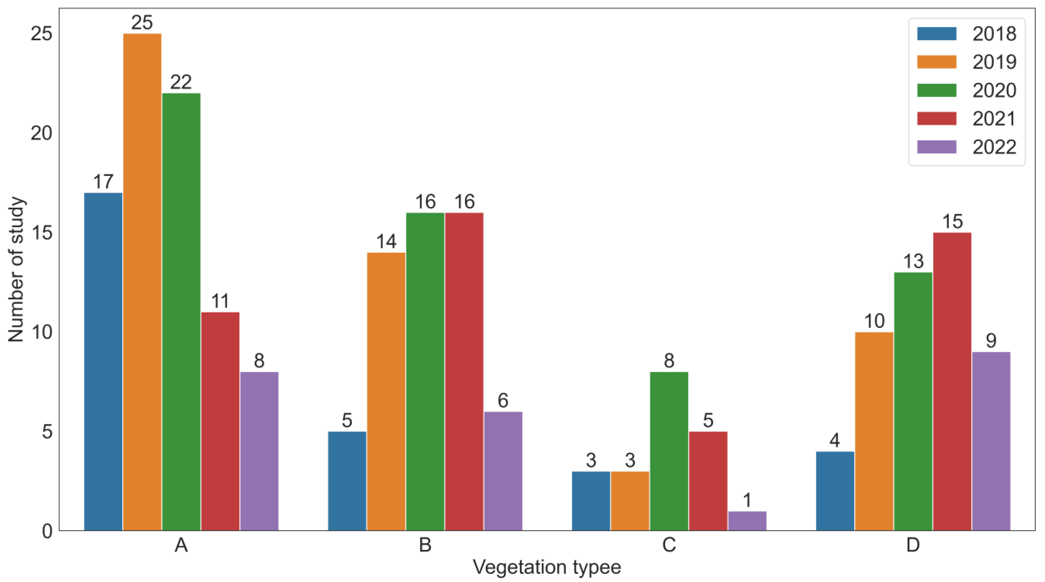
Figure 1. The number of published papers included in this literature review by vegetation type and by year. (A) forest, (B) vertically growing crops, (C) horizontally growing crops, and (D) grasses.
Remotesensing 15 03543 g001
Figure 2. Vegetation-based distribution of UAS platforms used to estimate above-ground biomass used on this literature review: (A) forest, (B) vertically growing crops, (C) grasses, and (D) horizontally growing crops.
Remotesensing 15 03543 g002
Figure 3. Frequency of using different sensors (red-green-blue (RGB), LIDAR, multispectral (MS), and hyper spectral (HS)) to estimate AGB in different vegetation types ((A) forest, (B) vertically growing crops, (C) horizontally growing crops, and (D) grasses).
Remotesensing 15 03543 g003
Figure 4. Frequency of using different flight altitudes (above ground level or AGL) used for each vegetation types is presented as a percentage ((A) horizontally growing crops, (B) vertically growing crops, (C) forests, and (D) grasses).
Remotesensing 15 03543 g004
Figure 5. The relationship between flight altitude in meter (above ground level) and the coefficient of determination (R2) of AGB estimation models in four group of crops. (A) Horizontally growing crops, (B) vertically growing crops, (C) forests, and (D) grasses.
Remotesensing 15 03543 g005
Figure 6. A comparison between flight altitude (meter above ground level) and sensor type (a), and side (b) and forward (c) overlap.
Remotesensing 15 03543 g006
Figure 7. The frequency distribution of different flight speed (m s−1) used for each vegetation types is presented as a percentage ((A) horizontally growing crops, (B) vertically growing crops, (C) forests, and (D) grasses).
Remotesensing 15 03543 g007
Figure 8. The comparison of accuracy of AGB estimation at two flight speed (less than or equal to 5 m s−1 and greater than 5 m s−1) in four types of vegetation (A) forest, (B) horizontally growing crops, (C) vertically growing crops, and (D) grasses).
Remotesensing 15 03543 g008
Figure 9. A comparison between flight speed (m s−1) and sensor type (a), and flight altitude (meter above ground level) (b).
Remotesensing 15 03543 g009
Figure 10. The frequency of using different forward overlap class used for each vegetation types is presented as a percentage ((A) horizontally growing crops, (B) vertically growing crops, (C) forests, and (D) grasses).
Remotesensing 15 03543 g010
Figure 11. The comparison of accuracy of AGB estimation between two overlap categories (less than or equal to 60% and greater than 60%) for side (i) and forward (ii) overlap in four vegetation types (A—forest, B—horizontally growing crops, C—vertically growing crops, and D—grasses).
Remotesensing 15 03543 g011
Figure 12. A comparison between side (a) and forward (b) overlap (%) and type of sensor (a).
Remotesensing 15 03543 g012
Figure 13. Frequency of using different number of ground control points (GCPs) used for each vegetation type is presented as a percentage ((A) horizontally growing crops, (B) vertically growing crops, (C) forests, and (D) grasses).
Remotesensing 15 03543 g013
Figure 14. The relationship between number of ground control points (GCPs) and the coefficient of determination (R2) of AGB estimation models in four groups of vegetations. (A) horizontally growing crops, (B) vertically growing crops, (C) forests, and (D) grasses. The blue lines represent a trendline or line of best fit.
Remotesensing 15 03543 g014
Figure 15. The comparison between number of ground control points (GCPs) at different sensors (a), flight speeds (b), and flight altitude (c).
Remotesensing 15 03543 g015
Figure 16. The frequency of different acquisition time of image to estimate the biomass in different groups of crops (A) forest, (B) vertically growing crops, (C) horizontally growing crops, and (D) grasses).
Remotesensing 15 03543 g016
Figure 17. The impact of the quantity of vegetation indices on the accuracy of AGB estimation in four vegetation types ((A) forest, (B) horizontally growing crops, (C) vertically growing crops, and (D) grasses).
Remotesensing 15 03543 g017
Figure 18. Use of different plant height metrics to estimate the biomass in different vegetation types ((A) forests, (B) vertically growing crops, (C) horizontally growing crops, and (D) grasses).
Remotesensing 15 03543 g018
Figure 19. Frequency distribution of feature selection methods (Fi—Filter methods, Wr—wrapper methods, and Em—embedded methods) for above-ground biomass estimation in various vegetation groups ((A) forests, (B) vertically growing crops, (C) horizontally growing crops, and (D) grasses).
Remotesensing 15 03543 g019
Figure 20. The performance of regression and machine learning models to estimate the AGB in four vegetation types ((A) forest, (B) horizontally growing crops, (C) vertically growing crops, and (D) grasses).
Remotesensing 15 03543 g020
Table 1. Keyword combination used during the literature search process for this review.
OrderKeywords
1above-ground biomass estimation
2above-ground biomass estimation, UASs, flight parameters, sensors
3above-ground biomass estimation, variables
4above-ground biomass estimation, modeling, machine learning
5above-ground biomass estimation, LIDAR
Table 2. Summary of focus of previous literature review papers on AGB estimation using UASs.
Focus of StudyReferences
Effective factors in estimating AGB using UASs[2,58]
Applications of UAS in crop biomass monitoring[18,55,57,59,65]
Developing the AGB estimation methods using remote sensing[56,64]
Flying sensors, challenges, and future directions[62]
Table 3. Most used sensors for AGB estimation and their applications.
SensorDescriptionCommon Application in AGB EstimationReferences
RGBVisible red, green, and blue informationManual digitizing of vegetation boundaries[65,89,90]
Calculating a range of RGB-based vegetation indices[38,47,91]
Creating a digital terrain model (DTM)[37,92]
Creating digital surface model (DSM) to determine canopy volume and canopy height model (CHM)[46]
MultispectralFive bandpass interference filters: red, green, blue, red-edge, and near-infraredCalculating a wide range of vegetation indices[70,93]
Creating DTM[26,73]
Creating DSM to determine canopy volume and canopy height model (CHM)[75]
HyperspectralMore bandpass compares to multispectralCalculating a wide range of multispectral vegetation indices[4,38,94]
LIDARRapid laser pulses to map the Earth’s surfaceCreating an RGB othomosaic[95]
Creating a more accurate DTM[87]
Creating a more accurate DSM to calculate canopy volume and CHM[48,81]
Table 4. Flight parameter thresholds in each sensor and vegetation type to estimate the above-ground biomass.
VegetationSensorFlight
Altitude (m)
Flight Speed
(m s−1)
Forward
Overlap %
Side
Overlap %
GSD
(m)
No. GCPR2References
ForestsRGB25–9504–4070–9050–900.015–16–810.56–0.96[25,35,37,40,44,52,92,104,129,130,131,132,133,134,135,136]
LIDAR40–40915–9250–8530–800.02–0.50.65–0.97[3,33,36,43,46,49,118,137,138,139,140,141,142,143]
MS/HS50–9005–5550–7550–65NAN0.56–0.87[144,145,146]
Vertically growing
crops
RGB15–1200.5–980–9060–900.049–0.1254–250.67–0.78[15,24,42,45,47,48,71,76,94,121,126,147,148,149,150,151,152,153]
LIDAR40–13005–6060–7070–900.02–0.50.89–0.9[30,81,154,155]
MS/HS1.3–1206–8575–9070–900.013–0.060.67–0.96[34,73,75,123,156,157,158,159,160]
Horizontally growing
crops
RGB13–302–570–8060–800.005–0.024–300.69–0.97[11,13,14,31,70,74,77,125,161,162,163,164,165]
LIDAR30–406–1550–7050–70-0.72–0.81[116,166,167]
MS/HS10–502–1060–8060–650.0085–0.0310.71–0.9[31,164,168,169,170]
GrassesRGB10–191.8–870–9060–850.004–0.394–600.54–0.98[17,32,38,91,120,171,172,173]
LIDAR5–253–10--0.003–0.110.71–0.73[83,87,95,174]
MS/HS50–1303–570–8065–800.017–0.10.62–0.93[72,122,175,176]
Table 5. Summary of image textural metrics, their types, and corresponding descriptions used in the above-ground biomass estimation literature.
MethodTypesDescriptionReferences
Co-occurrence matrixEnergyMeasures uniformity in grey level distribution of an image[74,188]
EntropyMeasures texture complexity[189]
ContrastMeasures difference in grey levels of an image[190]
HomogeneityMeasures similarity between pairs of pixels in an image[147]
CorrelationMeasures statistical relationship between pairs of pixels in an image[74]
Gabor filtersFrequencyNumber of cycles of a pattern present in an image[191]
OrientationAngle at which a pattern is oriented in an image[192]
ScaleSize of the pattern present in an image[147]
Local Binary
Patterns (LBP)
Uniform LBPBased on number of transitions between pixels of different intensities[193]
Non-uniform LBPConsiders the intensity values of pixels[194]
Rotation invariant LBPNot affected by rotation[195]
Fractal
Dimension
Box-counting dimensionBased on number of boxes needed to cover the image[185,189]
Information dimensionBased on amount of information contained in the image[196]
Hausdorff dimensionBased on degree of overlap between different parts of the image[197]
Table 6. The main parameters, advantages, and disadvantages of most used models (MLR—multiple linear regression, ANN—artificial neural network, RF—random forest, and SVM—support vector machine) to estimate the above-ground biomass.
ModelMain ParametersAdvantageDisadvantageReferences
MLRFitting linear relationship between variablesAllows multiple factors for dependent variableLinear relationship assumption may not hold[43,44,75,91]
Identify relative importance of independent variablesLess interpretable, sensitive to outliers
Latent variables representing relationshipsEffectively handles multicollinearity
ANNNumber of layersHandles large and complex datasetsComputationally intensive for large datasets[75,81,225]
Number of neurons in each layerAdapts and learns with new dataSensitive to initial conditions, overfitting
Activation function (sigmoid, tanh, ReLU)Handles non-linear relationships in dataDifficult to interpret, understand
Training algorithm (backpropagation, SGD)
RFNumber of treesSimple to implement, quick to trainNot good with missing values[50,73,144,226,227,228]
Decision tree depth limitRarely overfits, performs wellNot good for handling imbalanced data
Minimum samples to split nodeHandles large and complex datasets
Handles non-linear relationship
SVMKernel function classification typesHandles large complex datasetSensitive to kernel choice[33,45,75,229,230,231]
Regularization parameter controlHandles non-linear relationship
Kernel parameter tuningEffective in high-dimensional spaces
Table 7. Recommendations for Enhancing Accuracy in AGB Estimation: Effective Measures for Different Vegetation Types.
VTTBSFlight Altitude (m)Flight Speed (m s−1)Forward Overlap (%)Side Overlap (%)No. GCPFlight TimeNo. VIsTBHMTBFSMTBEM
ForestLIDAR100157065812–2 pm5MaximumVIFLR
Vertically growing cropsMS and RGB5058075712–2 pm10MaximumPCARF
Horizontally growing cropsRGB5058075512–2 pm10MeanRFERF
GrassesMS and RGB5058075512–2 pm10Mean and medianRFERF
Note: the presented values for number of GCPs and vegetation indices are the minimum values for these items. VT—vegetation type, TBS, the best sensor, VIs—vegetation indices, TBHM—the best height metric, TBFSM—the best feature selection method, TBEM—the best estimation model, MS—multispectral, RGB—red, green, blue, VIF—variance inflation factor, PCA—principal component analysis, RFE—recursive feature elimination, LR—linear regression, and RF—random forest.
Disclaimer/Publisher’s Note: The statements, opinions and data contained in all publications are solely those of the individual author(s) and contributor(s) and not of MDPI and/or the editor(s). MDPI and/or the editor(s) disclaim responsibility for any injury to people or property resulting from any ideas, methods, instructions or products referred to in the content.