Article

Novel Hybrid Model to Estimate Leaf Carotenoids Using Multilayer Perceptron and PROSPECT Simulations

1
School of Computer Science, Peking University, Beijing 100871, China
2
School of Geography and Information Engineering, China University of Geosciences, Wuhan 430074, China
3
Suzhou Enterprise Credit Service Co., Ltd., Suzhou 215000, China
4
International Institute for Earth System Science, Nanjing University, Nanjing 210023, China
*
Author to whom correspondence should be addressed.
Remote Sens. 2023, 15(20), 4997; https://doi.org/10.3390/rs15204997
Submission received: 26 July 2023 / Revised: 25 September 2023 / Accepted: 13 October 2023 / Published: 17 October 2023
(This article belongs to the Special Issue Vegetation Biophysical Variables and Remote Sensing Applications)

Abstract

:
Leaf carotenoids (Cxc) play a crucial role in vegetation as essential pigments responsible for capturing sunlight and protecting leaf tissues. They provide vital insights into a plant physiological status and serve as sensitive indicators of plant stress. However, remote sensing of Cxc at the leaf level has been challenging due to the low Cxc content and weaker absorption features compared to those of chlorophylls in the visible domain. Existing vegetation indices have been widely applied but often lack a solid physical foundation, which limits their applicability and robustness in characterizing Cxc. Yet, physical models can confront this ill-posed problem, though with high operational costs. To address this issue, this study presents a novel hybrid inversion method that combines the multilayer perceptron (MLP) algorithm with PROSPECT model simulations to accurately retrieve Cxc. The effectiveness of the MLP method was investigated through comparisons with the classical PROSPECT model inversion (look-up table [LUT] method), the convolutional neural network (CNN) hybrid model, and the Transformer hybrid model. In the pooled results of six experimental datasets, the MLP method exhibited its robustness and generalization capabilities for leaf Cxc content estimation, with RMSE of 3.12 μg/cm2 and R2 of 0.52. The Transformer (RMSE = 3.14 μg/cm2, R2 = 0.46), CNN (RMSE = 3.42 μg/cm2, R2 = 0.28), and LUT (RMSE = 3.82 μg/cm2, R2 = 0.24) methods followed in descending order of accuracy. A comparison with previous studies using the same public datasets (ANGERS and LOPEX) also demonstrated the performance of the MLP method from another perspective. These findings underscore the potential of the proposed MLP hybrid method as a powerful tool for accurate Cxc retrieval applications, providing valuable insights into vegetation health and stress response.

1. Introduction

Vegetation covers almost 70% of the earth’s land surface, and plant leaves are their primary photosynthetic organs [1,2]. Carotenoids (Cxc), including carotenes and xanthophylls, are crucial structural components of photosynthetic membranes [3,4]. They not only participate in light harvesting and energy transfer but also protect reaction centers and prevent photodamage to leaf tissue by dissipating excess energy [5]. Moreover, Cxc provide valuable information about plant growth, nutritional status, and the degree of damage to vegetation [6]. Hence, the accurate estimation of leaf Cxc plays a crucial role in monitoring the health status of vegetation and its functional diversity.
The labor-intensive and destructive nature of laboratory quantitative analyses makes them impractical for the large-scale monitoring of leaf biochemistry [7]. Fortunately, the development of remote sensing spectroscopy has made it possible to retrieve biochemical information quickly and non-destructively from intact leaves [8]. The methods for estimating leaf biochemical constituents can be broadly divided into two categories: empirical methods and physical models [9].
Empirical methods for estimating leaf biochemical content include models based on vegetation indices [10,11,12] and machine learning algorithms [13,14,15,16,17]. These methods establish empirical relationships between biochemical properties and leaf optics [18]. Although these data-driven methods are computationally efficient and can achieve promising accuracy for specific plant species, their effectiveness heavily depends on the quality and variability of the training data. Furthermore, they lack generalization for different vegetation species and environmental conditions without sufficient representative data [19].
Physically based modeling approaches, also known as radiative transfer models (RTMs), have been proposed to retrieve biochemical contents in a wide range of species and living conditions, achieving good physical interpretations and satisfactory transferability by simulating the process of radiation transmission [20,21,22]. The PROSPECT model [23,24] is the most popular leaf optical property model. However, the ill-posed nature of the inversion and computational inefficiency are the main drawbacks of physical models, limiting their practical application for regional or global studies [25].
Novel hybrid methods [26,27,28,29,30], which combine data-driven methods with RTMs [31], have been developed to address these issues. With training data simulated by RTMs, a variety of machine learning algorithms [32], such as Gaussian process regression [33,34], random forest regression [35], support vector machine regression [36], and artificial neural network (ANN) [37,38], can be used for biochemical and biophysical vegetation property retrieval studies. These hybrid methods can achieve promising accuracy and efficiency while improving generalization, as they benefit from sufficient non-destructive synthetic data for training.
The absorption peaks of chlorophyll (Chl) and Cxc are in similar spectral ranges, but the content of Chl in the leaves is much higher than that of Cxc. Thus, the estimation of the leaf Cxc content is confounded by the leaf Chl content. Studies on the retrieval of the total Chl content of leaves using various inversion methods have achieved satisfactory accuracy [39,40], while studies on Cxc are scarce, and the performance achieved falls short of expectations for the reasons introduced above [8]. Traditionally, look-up tables (LUTs) have been widely employed for Cxc content inversion. However, the inherent non-linearity of the relationship between spectral reflectance and Cxc content poses a substantial challenge. LUTs may struggle to account for the intricate interplay between Cxc and other constituents, particularly Chl, causing inaccuracies in Cxc content estimation. In light of these challenges, alternative approaches such as multilayer perceptrons (MLPs) [41] offer a promising avenue to enhance the precision of Cxc content estimation, thanks to their capacity to model complex non-linear relationships [42,43] and adapt to varying scenarios [44]. Through parameter optimization during training, an MLP fine-tunes its internal parameters for target trait estimation. Thus, the MLP method holds great potential to distinguish the contribution of leaf Cxc from the interference of leaf Chl.
In recent years, domain-specific neural network architectures, such as the convolutional neural network (CNN) for image processing [45,46] and the Transformer model for natural language processing [47,48], have achieved significant advancements and impressive results in their respective domains. Given the success of these architectures in handling specific data types, investigating their potential effectiveness in the context of Cxc content inversion is essential. In this research, we introduce CNN and Transformer as alternative ANN architectures to MLP, as well as PROSPECT model inversion, which has often been used for Cxc inversion. By comparing their performances on the same datasets, we aimed to gain insights into how each model handled the complexity of spectral reflectance data and its ability to accurately predict the Cxc content.
The main objective of this study was to develop a robust and accurate method for estimating leaf Cxc content by combining the MLP with the PROSPECT model. The robustness and generalizability of the proposed method were tested by evaluating the model on six diverse leaf datasets encompassing various plant species and physiological states. Furthermore, a comparative analysis was conducted between the MLP hybrid model and a traditional physical model inversion method, as well as two hybrid methods based on domain-specific neural network architectures (CNN and Transformer). This analysis could provide valuable insights into the strengths and limitations of the MLP approach compared with other state-of-the-art techniques.
The remainder of this article is organized as follows. Section 2.1 and Section 2.2 introduce the construction of synthetic datasets for model training and the development of the MLP. Section 2.3 introduces the main characteristics of the six independent datasets for model testing. Section 2.4 presents two quantitative indicators for model evaluation. Section 2.5 describes three alternative methods for comparison. Section 3 presents the estimated Cxc results. Section 4 analyzes the experimental results and discusses a comparison with the existing literature, along with the constraints and future prospects of this study. Finally, Section 5 presents the conclusion of this study.

2. Materials and Methods

This study’s workflow began with the generation of a synthetic training dataset using the PROSPECT model’s forward mode, serving as the foundation for training the MLP model (Figure 1). Subsequently, the trained MLP model was applied to real-world scenarios, utilizing diverse datasets, including ANGERS, LOPEX, NX, XS, BM, and JTL, which offer a wide range of species for comprehensive validation. To provide a thorough analysis, we conducted a comparative evaluation involving alternative inversion techniques, such as look-up table (LUT)-based model inversion, the CNN hybrid model, and the Transformer hybrid model. Notably, both CNN and Transformer, being part of the family of artificial neural networks (ANNs), follow a model inversion process similar to the one depicted in Figure 1.

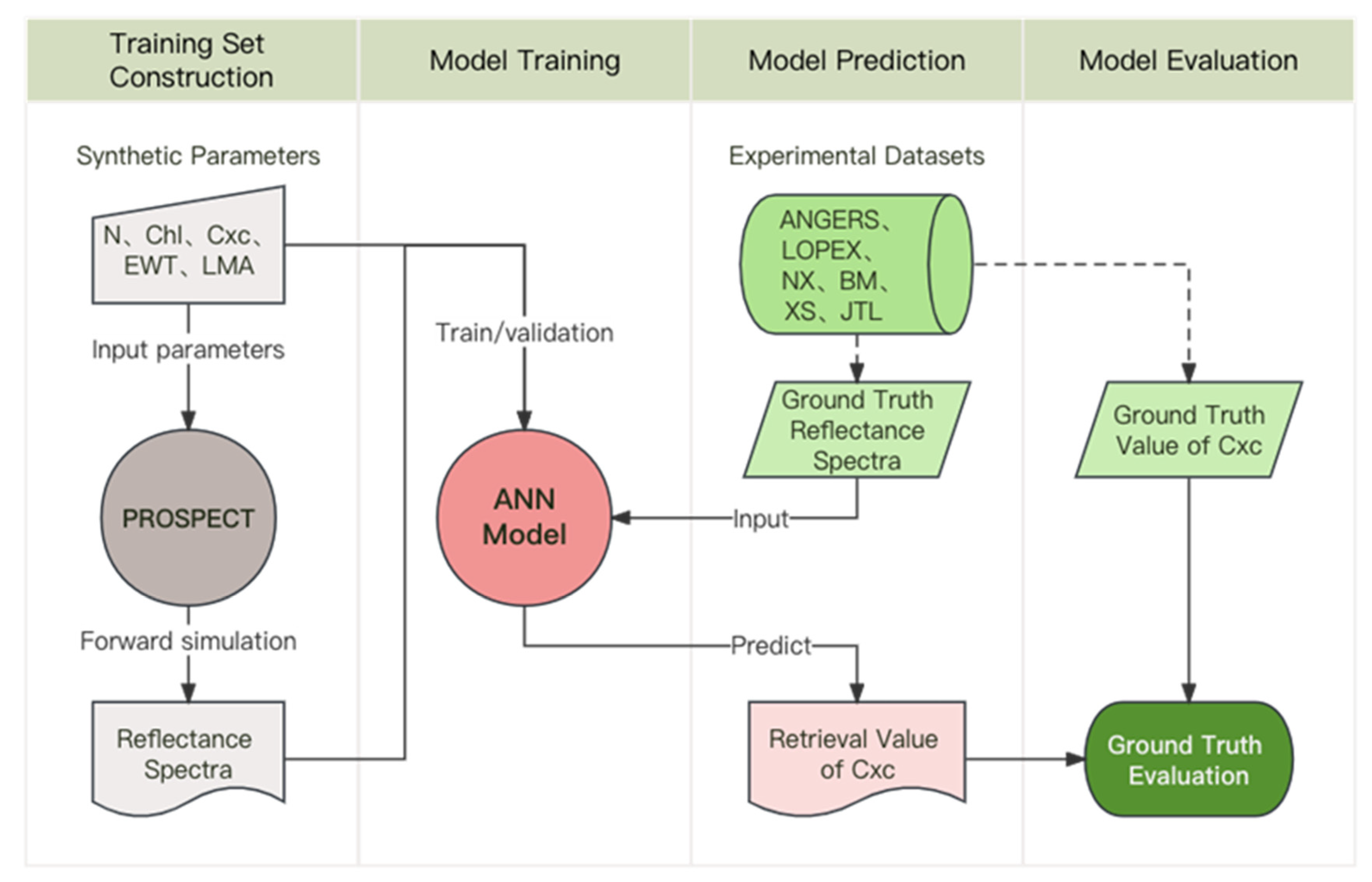
2.1. Training Set Construction: Simulated Data

In the forward mode, the PROSPECT model simulated leaf directional–hemispherical reflectance and transmittance, referred to as reflectance and transmittance hereafter, from 400 nm to 2500 nm with input biochemical contents per unit of leaf surface and the leaf structure parameter (N), which accounts for the mesophyll structure [23]. In the inverse mode, PROSPECT could estimate the leaf biochemical parameters from the observed spectral data. Various versions and extensions of the PROSPECT model have been introduced in the literature [49], and Cxc were first included in the fifth version, PROSPECT-5 [50].
The MLP model requires a substantial amount of training sample data consisting of leaf reflectance spectra and corresponding biochemical parameters to accurately estimate Cxc from leaf reflectance spectra. This was necessary to effectively approximate the relationship between the two. Representative leaf reflectance data were simulated by running the PROSPECT-5 model in the forward mode to meet the training quantity and quality requirements.
The construction of the synthetic dataset involved two steps. First, a total of 11,000 sets of leaf biochemical parameters were randomly drawn from a multivariate Gaussian distribution [51]. Among these, 10,000 sets were used for training and validation of the model, while the remaining 1000 sets were reserved for accuracy testing of the MLP model. The realistic ranges and distributions of these parameters (listed in Table 1) were defined based on previous studies [52,53,54]. In addition, strong correlations reported in the literature [55,56] between parameters such as leaf Chl and Cxc (R2 = 0.86), as well as leaf mass per area and equivalent water thickness (R2 = 0.63), were taken into account during this step. Then, the PROSPECT model was executed in the forward mode to generate the corresponding leaf reflectance spectra by utilizing the leaf biochemical parameters obtained in the first step as input. The biochemical parameters and their corresponding spectral data generated through these two steps collectively formed the synthetic dataset used for model training in this study.

2.2. Model Training: Multilayer Perceptron

2.2.1. Model Description

Technological advancements have led to the development of ANNs from shallow neural networks to deep learning neural networks (DNNs) [57]. DNNs contain multiple non-linear layers that can learn complex functions by transforming representations from one level to a higher, more abstract level through simple but non-linear modules. DNNs can automatically extract deeper features through this general-purpose learning procedure and are therefore better equipped than conventional machine learning techniques to process raw natural data, which require engineering skills and domain expertise to design feature extractors [58,59].
The MLP is a powerful DNN model widely used in machine learning and renowned for its simplicity and efficiency [60]. It emulates the structure and information processing of neural networks in the human brain. The MLP consists of interconnected nodes that apply activation functions to transform inputs into outputs. It has multiple layers, including an input layer, one or more hidden layers, and an output layer [61]. The MLP excels at automatically extracting relevant features from data, eliminating the need for extensive manual feature engineering. This feature makes it well suited for tasks such as leaf functional traits retrieval. By leveraging the backpropagation algorithm [62], the MLP can learn complex relationships between input features and target variables.

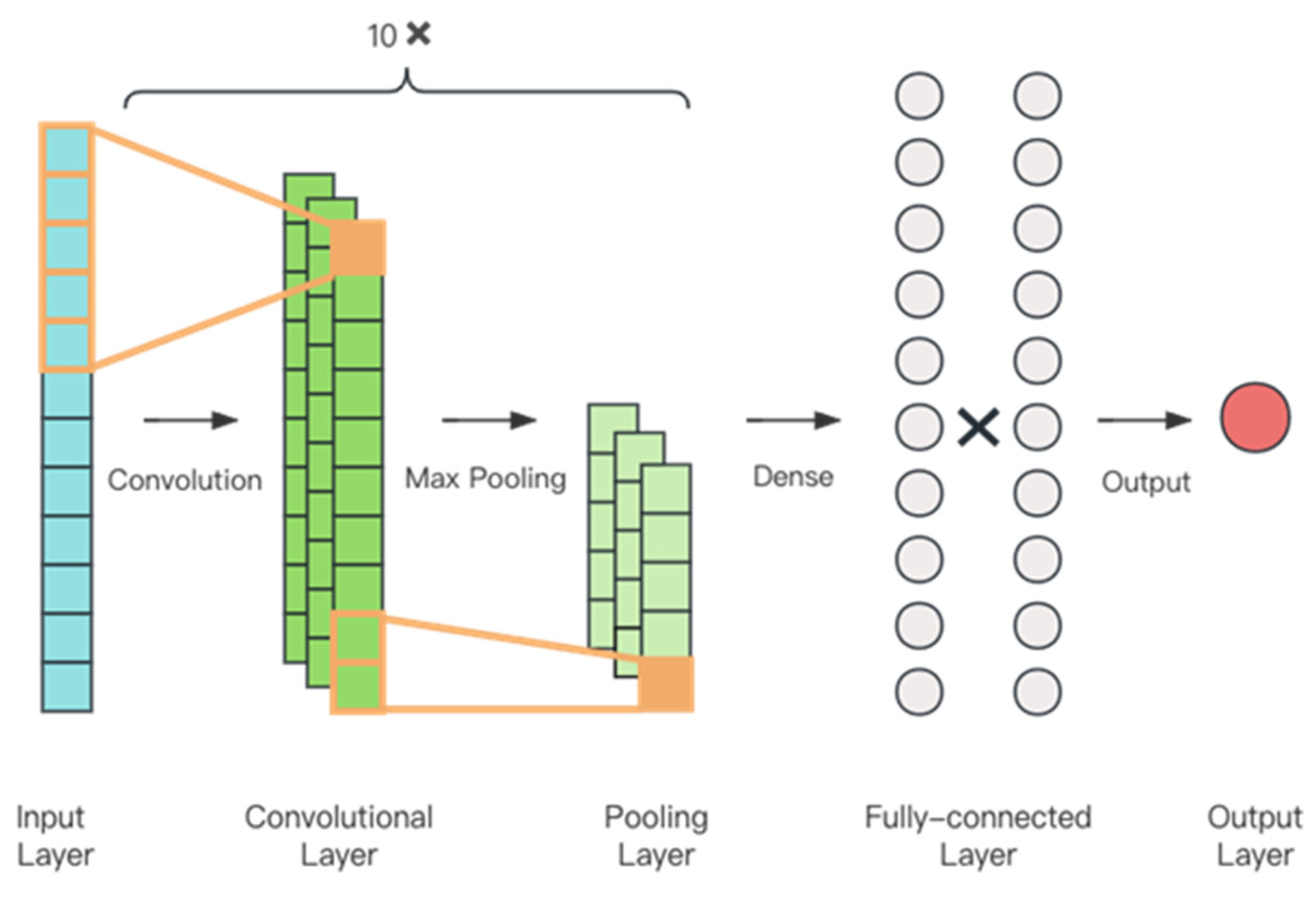
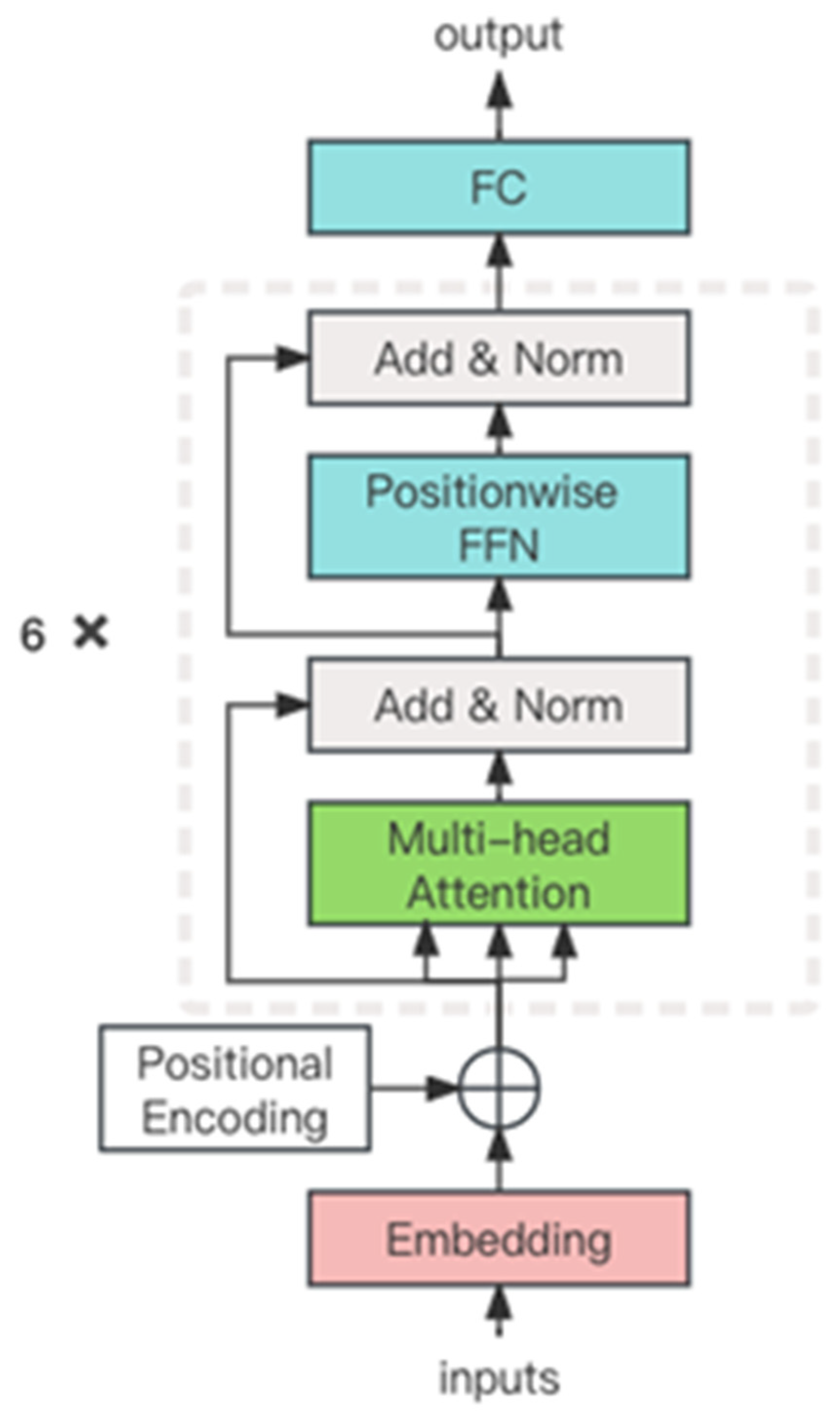
2.2.2. Model Architecture

In this study, we employed a five-layer neural network architecture, as depicted in Figure 2. The network consisted of three hidden layers with 512, 256, and 128 nodes, respectively. The output layer consisted of a single node, which was responsible for producing the estimated value of Cxc. The input layer had 512 nodes, each representing a specific wavelength within the 400–911 nm reflectance spectrum.
The use of the 400–911 nm spectral range was driven by several considerations. Firstly, the 400–911 nm wavelength range covers a broad spectrum sensitive to both Cxc and Chl [63,64]; the latter is strongly correlated with the Cxc content. Beyond the visible range, the absorption diminishes, resulting in reduced sensitivity to Cxc levels. Secondly, the choice of using a power-of-two number of data points (512) offered computational efficiency advantages for the MLP. Many deep learning frameworks and hardware architectures are optimized for power-of-two dimensions, resulting in faster and more efficient calculations. Thirdly, a narrow spectral range simplifies data processing, feature extraction, and the design of neural network structures. In contrast, a wide spectral range would require more complex processing and could lead to increased computational costs and complexity.
The activation function used in the hidden layers was the scaled exponential linear unit (SELU) [65]. SELU has shown effectiveness in DNNs, addressing the vanishing/exploding gradient problem and promoting self-normalization. It helps stabilize the learning process and improves the overall performance of the model [66,67]. For model optimization, the Adam [68] algorithm was utilized, which is an adaptive learning rate optimization method. The learning rate was set to 1 × 10⁻⁶, allowing the precise adjustments of the model’s weights during training. The model was trained for 1500 epochs, and a batch size of 128 was used during the training process. The MLP model was implemented in Python and executed on a machine with eight cores and an NVIDIA GeForce GTX 1080 Ti GPU. During the training process, the training data inputs were randomly shuffled and divided into a training set (75%) for model training and a validation set (25%) for hyperparameter tuning.

2.3. Model Prediction: Experimental Datasets

In this study, a diverse dataset consisting of fresh leaf samples from six independent datasets collected in different locations and growth stages was utilized. These datasets encompass a wide range of species and physiological statuses, including dicotyledon and monocotyledon, annual and perennial plants, and trees and herbs.
LOPEX [69] and ANGERS [50] are public datasets that are widely used for leaf model calibration and validation. The ANGERS leaf database comprises a total of 276 leaves sourced from 43 herbaceous and woody plant species. The LOPEX dataset consists of 330 leaves representing 46 plant species. These two datasets are available online (https://ecosis.org/package/angers-leaf-optical-properties-database--2003-, https://ecosis.org/package/leaf-optical-properties-experiment-database--lopex93- accessed on 10 May 2023) and were thus often used in previous studies [40,49,50,52,70], which offered us a valuable opportunity to compare our results with the results of these studies. The XS, NX, BM, and JTL datasets were obtained from field campaigns conducted near Nanjing (Jiangsu Province, Eastern China) between 2014 and 2015. Top-of-canopy leaf samples were collected at various stages during the growing seasons. The XS and NX measurements were taken from leaf out to leaf fall, covering the entire growing season in 2014. The leaves in BM were measured in the summer of 2015. The JTL samples were collected in May and July of 2015 from an evergreen forest, including both current-year and second-year or older leaves. The key characteristics of the six datasets are summarized in Table 2. Comprehensive information about vegetation species and leaf measurement methods can be found in [71]. The leaf reflectance spectra were measured using spectroradiometers coupled with integrating spheres, and the spectral resolution was 1 nm for all datasets. Only reflectance wavelengths ranging from 400 nm to 911 nm were considered as inputs to ensure a fair comparison with the MLP model structure.

2.4. Model Evaluation

Two quantitative indicators, namely, the coefficient of determination (R2) and the root-mean-square error (RMSE), were calculated to assess the accuracy and generalizability of the proposed methods across diverse independent datasets with varying biochemical compositions. Let y j and y j represent the measured and estimated values, respectively; y ¯ denotes the average of y j , and n denotes the number of samples. The formulas for R2 and RMSE are as follows:
R 2 = 1 j = 1 n y j y j 2 j = 1 n y j y ¯ 2
R M S E = j = 1 n y j y j 2 n
These metrics provide a quantitative measure of how well the estimated values correspond to the measured values. A high R2 value indicates a good fit of the model to the data, while a low RMSE value signifies low prediction errors.

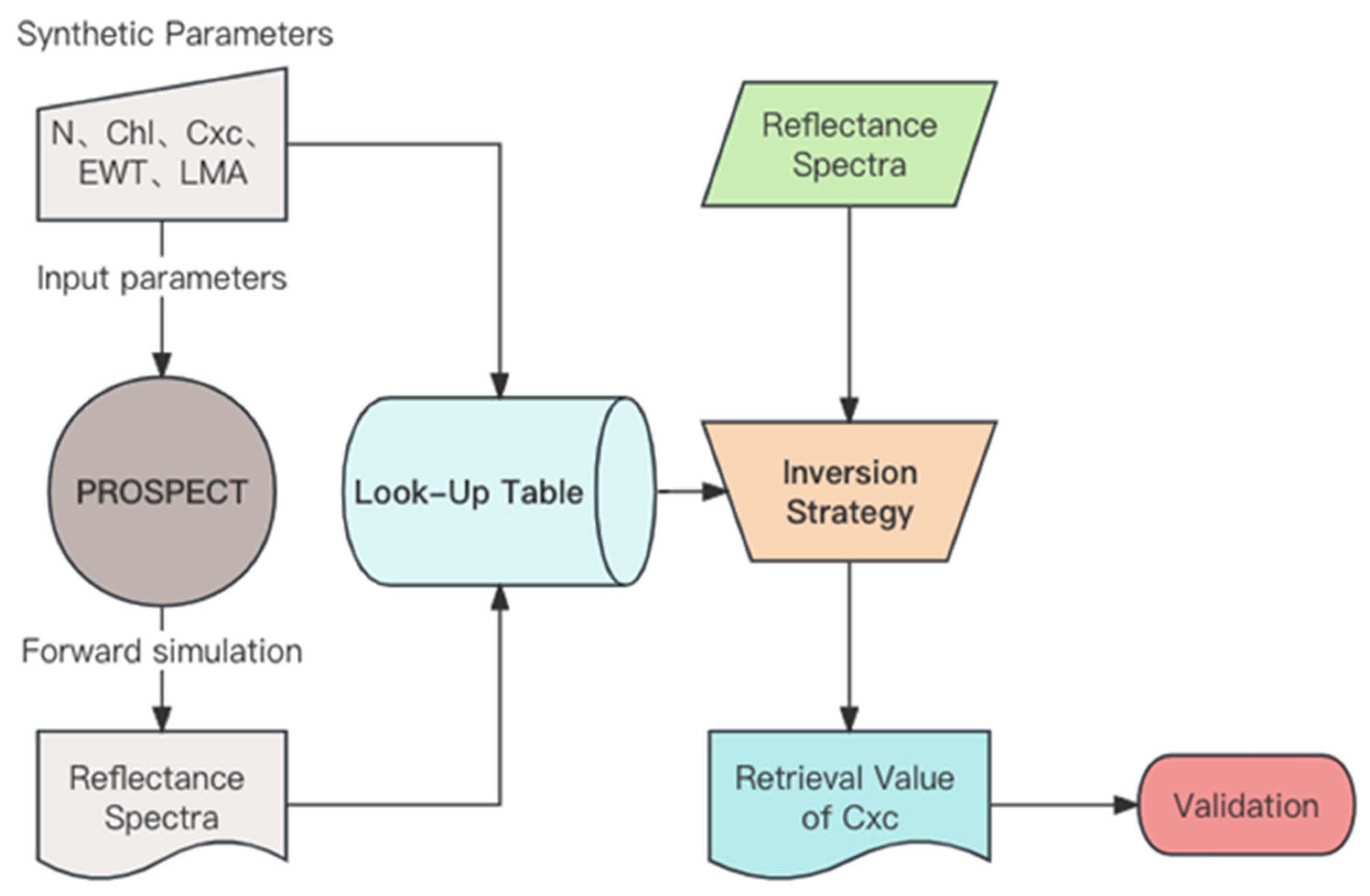
2.5. Alternative Inversion Methods for Comparison

Three inversion methods for leaf Cxc were compared with the MLP method in this study, namely, the LUT-based PROSPECT model inversion, the CNN hybrid model, and the Transformer hybrid model. Including the classic PROSPECT model inversion in the comparison allowed us to assess the performance of data-driven methods such as the MLP against this well-established physically based approach. Given the necessity for efficient feature extraction from sequential data, such as spectra, and the benefits of translation invariance, parameter sharing, and adaptability to diverse data scales, we considered the utilization of 1D CNNs to address Cxc inversion challenges. Leveraging Transformer architectures for inversion tasks was driven by their ability to efficiently capture complex dependencies in sequential data through self-attention. The capability to consider both local and global context makes Transformer promising for improving Cxc inversion models.
Physically based models can be inverted using two methods: iterative optimization and the LUT method. We used the LUT-based PROSPECT model inversion in this study because it is computationally more efficient than numerical iteration and avoids the problem of local minima [26,72]. As illustrated in Figure 3, PROSPECT model inversion based on a LUT involved precomputing a database of synthetic spectra covering a range of vegetation parameters. Actual spectral observations, typically from remote sensing data, were then compared with the LUT to identify the best-fitting parameters. The LUT established a relationship between leaf reflectance spectra and Cxc content, enabling Cxc inversion by looking up values in the table. The LUT generated in this study was composed of 100,000 entries. The setting of the model input parameters was in accordance with Table 1. The cost function of least-squares estimator was utilized, which assumes the maximum likelihood criterion [73].
The CNN is a powerful deep learning architecture that is widely used for image and sequence data processing tasks [74]. A CNN consists of multiple layers of learnable filters or kernels that convolve (apply sliding windows) over the input data to extract hierarchical features [75]. These features are progressively learned and combined through convolution, pooling, and nonlinear activation functions, allowing CNNs to automatically identify patterns and structures within data. The CNN used in this study consisted of 10 convolutional layers with a kernel size of 3 and 32 filters in each layer (Figure 4), followed by a fully connected layer with 256 units and a final output layer for regression. ReLU was used as the activation function, and max-pooling layers with a kernel size of 2 and dropout rates with a probability of 0.5 were applied for dimension reduction and regularization. The CNN model was trained using the Adam optimizer with a learning rate of 0.0001 and a batch size of 128 and ran for 20 epochs. The mean squared error (MSE) was used as the loss function.
The Transformer is a revolutionary deep learning architecture that excels in processing sequential data such as text and time series [76,77]. It relies on a mechanism called “self-attention”, which allows it to weigh the importance of different parts of the input sequence when making predictions [78]. Transformers process the entire sequence in parallel, facilitating scalability and capturing long-range dependencies efficiently [79]. This architecture has enabled significant breakthroughs in natural language processing and various other fields due to its superior ability to model complex relationships within data [80]. Our specific Transformer model comprised 6 layers of encoder blocks with 8 attention heads and 2 hidden layers of dimension 512 (Figure 5). We applied a dropout rate of 0.1 to prevent overfitting during training. For optimization, we used the Adam optimizer with a small learning rate of 1 × 10⁻⁶, which ensured efficient convergence. The model was trained for 100 epochs with a batch size of 128 samples.
Both CNN and Transformer models were trained following the flowchart illustrated in Figure 1 using the same simulated dataset as the one used for the MLP. All the four methods were evaluated on six diverse datasets, which were introduced in Section 2.3.

3. Results

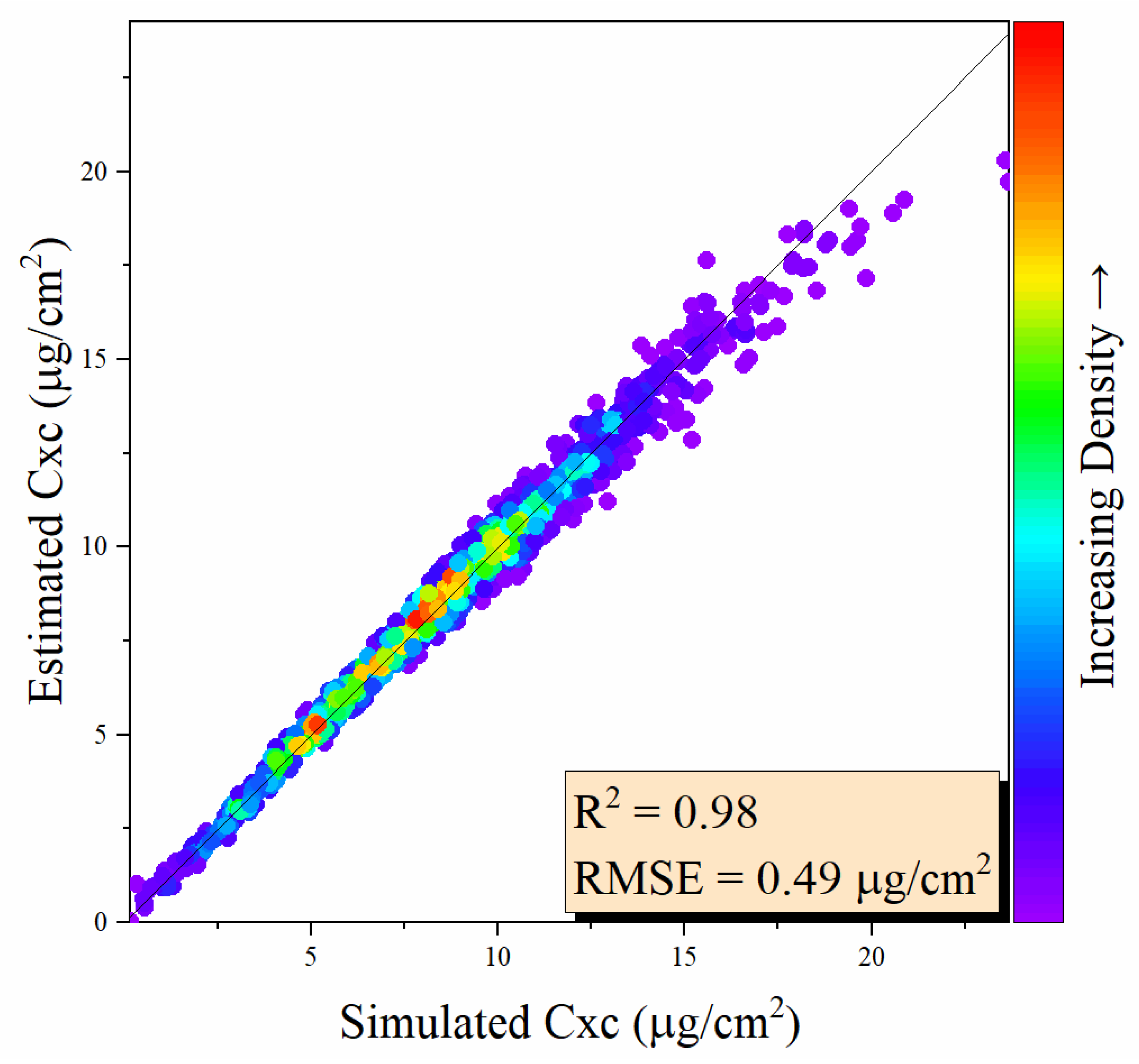
3.1. Performance of the MLP Model Using Simulated Data

In this section, we describe tests conducted on the MLP model that was constructed using a simulated test dataset containing 1000 data points based on PROSPECT model simulations to validate MLP’s effectiveness (Figure 6). The scatter plot illustrates that the sample values tightly aligned along the y = x line, indicating a strong correlation between predicted and actual leaf Cxc values. The highest density region on the plot is approximately in the range from 4 to 12 μg/cm2, indicating that the MLP model achieved better inversion results when the Cxc content lay within this range. When the Cxc content exceeded 16 μg/cm2, the density plot’s tail exhibited a slight divergence, thereby suggesting the Cxc tended to be underestimated at higher contents. Nevertheless, the model demonstrated overall excellent performance, with an RMSE of 0.49 μg/cm2 and a high R2 value of 0.98, which confirmed its effectiveness in accurately predicting the Cxc content.

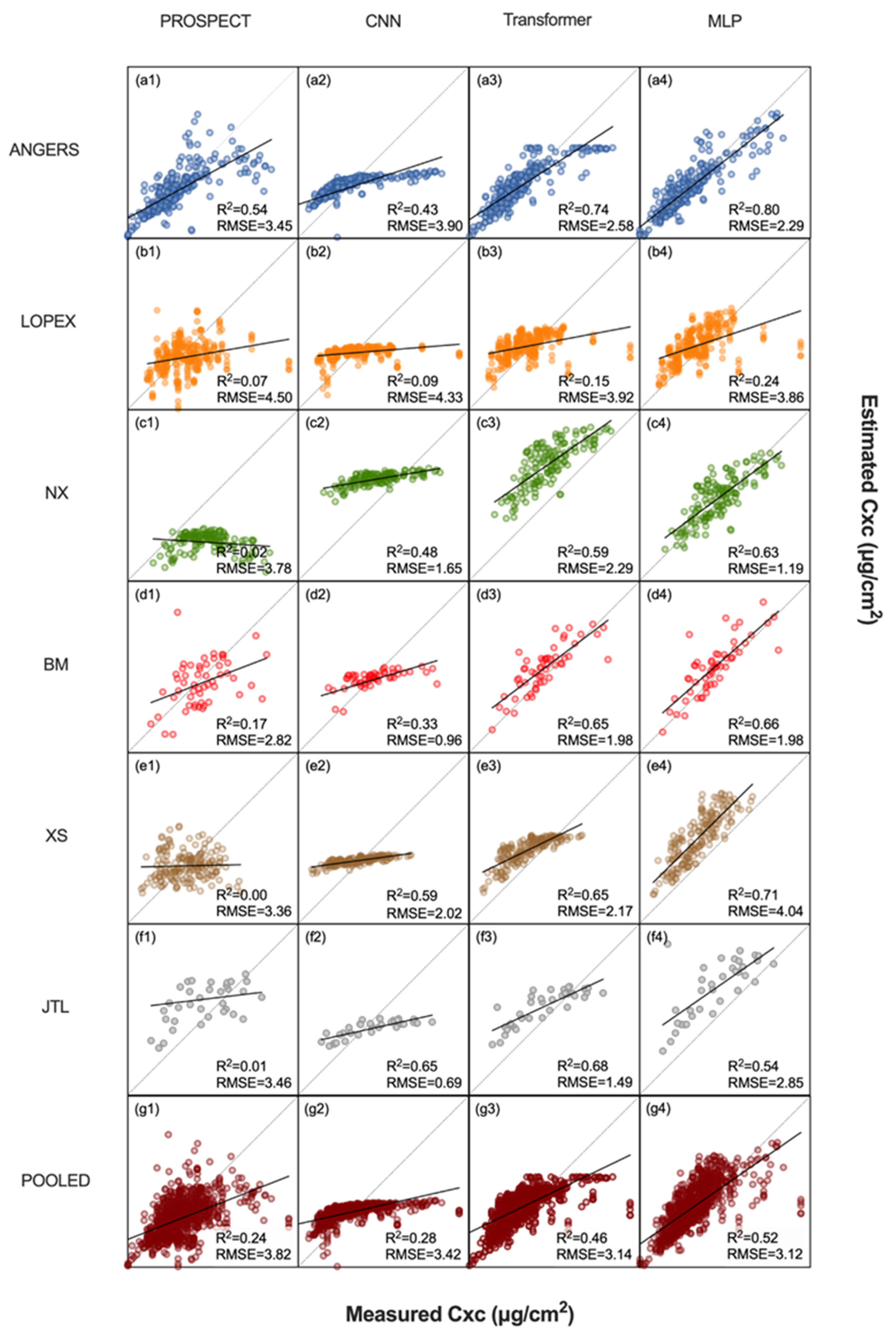
3.2. Performance of the MLP and Alternative Methods Using Experimental Datasets

The MLP method was tested on six different experimental datasets, namely, ANGERS, LOPEX, NX, BM, XS, and JTL. The evaluation aimed to assess the method’s ability to accurately estimate Cxc contents across diverse datasets, thereby confirming its robustness and generalization capabilities. To validate the effectiveness of the MLP method, we also conducted a comparative analysis against three well-established methods, namely, the LUT-based PROSPECT model inversion, the CNN-based hybrid method, and the Transformer-based hybrid method. This comparison proved the advantages and limitations of the MLP method in relation to other techniques for Cxc content inversion (Figure 7). The scatter plots in Figure 7 visually illustrate the performance of the leaf Cxc estimation using each method on the six datasets.
In the context of leaf Cxc estimation, the MLP method (Figure 7(a4–g4)) exhibited exceptional performance. The plotted points aligned closely with the y = x diagonal line across all datasets, indicating a robust fit between predicted and actual leaf Cxc contents. This alignment underscored the method’s ability to maintain a strong correspondence with the true values, even though minor deviations, suggesting a slight overestimation tendency, were observed in the datasets XS (Figure 7(e4)) and JTL (Figure 7(f4)). Nevertheless, these discrepancies were relatively small, affirming the MLP’s consistent and accurate performance across diverse datasets. This comprehensive analysis demonstrated MLP’s consistent superiority over PROSPECT model inversion, CNN, and Transformer, as evidenced by the lower RMSE values and higher R2 scores, particularly for the datasets ANGERS (Figure 7(a4)), LOPEX (Figure 7(b4)), and NX (Figure 7(c4)), with MLP R2 values of 0.80, 0.43, and 0.74, respectively, and RMSE values of 2.29, 3.90, and 2.58 μg/cm2, respectively. Thus, the MLP outperformed its counterparts.
For the PROSPECT model inversion, the scatter plots (Figure 7(a1–g1)) showed clustered points without clear alignment to the y = x line. This finding indicated that LUT struggled to capture the continuous relationship between spectral reflectance and Cxc contents, resulting in poor performance. For the NX (Figure 7(c1)) and XS (Figure 7(e1)) datasets in particular, the fitted line showed a negative trend, which indicated a failed inversion of the two datasets. The quantitative analysis confirmed these observations. The PROSPECT model exhibited overall inferior performance, with higher RMSE values and lower R2 scores, in all cases compared with the other methods.
The scatter plots for the CNN method (Figure 7(a2–g2)) exhibited a trend of a fitted line close to a horizontal orientation. This tendency suggests that CNN faced challenges in accurately estimating the Cxc contents, especially at higher content levels. The CNN showcased lower RMSE values on the BM (Figure 7(d2)), XS (Figure 7(e2)), and JTL (Figure 7(f2)) dataset. For instance, on BM, the CNN achieved the lowest RMSE of 0.96 μg/cm2, surpassing the MLP RMSE of 1.98 μg/cm2 (Figure 7(d4)). Although the CNN inversion achieved a low RMSE, a closer examination of the scatter plot revealed that the CNN’s inversion performance was not satisfactory. This observation was further supported by the relatively low R2 value obtained from the CNN’s predictions.
For the Transformer method, the scatter plots (Figure 7(a3–g3)) showed a performance closely approaching that of the MLP (Figure 7(a4–g4)). The points aligned relatively well with the y = x line, indicating competitive prediction accuracy. A quantitative analysis supported this observation of competitive performance, with the Transformer method sometimes surpassing the MLP in terms of R2 scores and RMSE. This was particularly evident in the case of the dataset JTL, on which the Transformer method (Figure 7(f3)) achieved an R2 of 0.68 and an RMSE of 1.49 μg/cm2. In contrast, the MLP (Figure 7(f4)) obtained an R2 of 0.54 and an RMSE of 2.85 μg/cm2 on the same dataset. Nevertheless, when the overall assessment of leaf Cxc was considered, as shown in the pooled dataset, the MLP (Figure 7(g3)) outperformed the Transformer (Figure 7(g4)).
Considering the pooled results of the six datasets, the MLP method outperformed all others, with RMSE of 3.12 μg/cm2 and R2 value of 0.52. Following were the Transformer (RMSE = 3.14 μg/cm2, R2 = 0.46), CNN (RMSE = 3.42 μg/cm2, R2 = 0.28), and LUT (RMSE = 3.82 μg/cm2, R2 = 0.24) methods, ranked in descending order of accuracy. As for the computational time cost, MLP, Transformer, and CNN required less than a second for the inversion of the pooled six datasets, while LUT required approximately 21 min. Consequently, in terms of inversion efficiency, the hybrid approaches based on ANN models (MLP, CNN, and Transformer) demonstrated significantly higher efficiency compared to the LUT-based approach.

4. Discussion

4.1. Comparison with Alternative Approaches

With regard to the retrieval effectiveness of leaf Cxc, the comparison between the MLP and other methods revealed the superiority of the MLP in conducting Cxc content inversion tasks. The consistent and accurate performance of the MLP across all datasets demonstrated its effectiveness in this domain. According to the pooled results from the six datasets, the MLP (Figure 7(g4)) outperformed in effectiveness the Transformer method (Figure 7(g3)), which outperformed the CNN (Figure 7(g2)). The LUT (Figure 7(g1)) lagged behind these three methods. Notably, the classic LUT-based PROSPECT model inversion showed subpar performance across all datasets, thus revealing the incompetence of this physical model in retrieving the Cxc content accurately. Although the adopted spectral range of 400–911 nm exceeded the absorption domain of Cxc and Chl and partly covered the sensitive range of leaf structure parameters, this relatively narrow range could have affected the inversion performance. As a complementary analysis, this study will further compare the MLP method with physical models reported in other relevant literature in Section 4.2. While both one-dimensional CNN and Transformer seem suitable for multi-input single-output problems, CNN appears more inclined to capture the spatial correlations among sequences, whereas Transformer excels in discovering semantic relationships [81,82]. However, such correlations and relationships may not be strongly present in spectral reflectance sequences, which may explain the fact that these methods did not surpass the MLP in performance. As a complementary analysis, this paper also references the results from a previous study on hybrid models based on CNNs in Section 4.2 for comparison and reference.
With regard to the retrieval efficiency of leaf Cxc, hybrid models such as the MLP exhibited remarkable efficiency once the model was established. They retrieved the pooled six datasets in less than one second, making them much faster in handling large-scale tasks. The high computational efficiency of ANN models results from the optimization of the models’ calculations and the ability to leverage hardware acceleration [83,84]. The ANN models consist of interconnected neurons, and their computations involve mathematical operations such as addition, multiplication, and activation functions, which are efficiently organized as matrix multiplications and vector operations [85]. In addition, deep learning frameworks optimize the computation graph automatically, adapting to available computing resources and enabling parallel processing and GPU acceleration [86,87].

4.2. Cxc Retrieval Accuracy in Comparison with Previous Studies

Many previous studies extensively investigated the retrieval of leaf Cxc contents by using PROSPECT model inversion [40,49,50,52,70]. Notably, the publicly available datasets ANGERS and LOPEX were widely utilized in these studies, thus allowing us to compare the results of our MLP-based approach with those of published studies on Cxc estimation.
To facilitate the comparison, we summarized the accuracies of the cited studies on ANGERS and LOPEX under various conditions in Table 3 and Table 4, respectively. An important detail to note is that the studies incorporating both leaf transmittance spectra and reflectance spectra in the inversion process should have achieved better accuracies theoretically, as they utilized a richer set of spectral information. We provided the RMSE values for all cited studies, and the R2 values were included if they were also reported. For comparison purposes, we also included the accuracies of our MLP method.
The first three studies in Table 3 employed direct iteration of the PROSPECT model inversion for Cxc retrieval, with their performance varying based on the model version and the use of spectral domain. Li et al. [70] introduced modifications to the PROSPECT model by coupling it with continuous wavelet transform. Shi et al. [40] proposed a hybrid method combining PROSPECT-5 with CNN.
For the ANGERS dataset (Table 3), our MLP method outperformed most of the cited studies, as evidenced by its lower RMSE value of 2.29 μg/cm2. Among the previous methods with reflectance alone, [70] the closest RMSE of 2.50 μg/cm2 was obtained with the modified PROSPECT model of PROCWT-S3. With regard to the R2 values, though [40] achieved a high R2 of 0.74 using PROSPECT-5, our MLP method attained R2 of 0.80, indicating a strong correlation between predicted and observed Cxc contents.
For the LOPEX dataset (Table 4), the performance of our proposed MLP method achieved a significant reduction in RMSE compared to all the cited studies. Specifically, the RMSE of the MLP decreased by 9.6% to 27.9% when compared with the RMSE values reported in previous studies.
The results in Table 3 and Table 4 clearly demonstrate that the performance of our MLP-based hybrid method was superior to those of the best-performing methods reported in the literature for the ANGERS and LOPEX datasets. Our MLP hybrid method utilizing reflectance within the 400–911 nm wavelength range proved effective and competitive in Cxc estimation, outperforming the cited methods based on physical models and the hybrid model based on CNN.
The improved performance of our MLP-based hybrid method highlights the effectiveness of the neural network approach in capturing complex patterns and relationships within spectral data, resulting in more accurate predictions of the Cxc content. This finding suggests that neural networks are advantageous for handling the intricate characteristics of spectral data, leading to enhanced estimation accuracy.
The substantial decrease in RMSE achieved by our MLP-based hybrid method indicates its potential as a powerful tool in remote sensing applications, especially for precise Cxc estimations. Its ability to obtain more reliable Cxc estimates has significant implications for agricultural and environmental research, facilitating better monitoring and management of plant health and stress levels.

4.3. Study Constraints and Future Prospects

While our study primarily underscored the MLP’s commendable performance on the majority of the examined datasets, overestimation of the Cxc content was evident for the JTL dataset (Figure 7(f4)), which suggests potential limitations of the proposed method for vegetation types such as Ligustrum lucidum L. (the only species in the JTL dataset [71]). In future work, additional datasets from various ecosystem types and growing conditions could be considered to validate the performance of the MLP-based hybrid method. Furthermore, beyond the Cxc retrieval, our method demonstrated potential in estimating other biochemical parameters, which requires further validation in subsequent studies. Our upcoming research will involve integrating the MLP with canopy-scale models [88,89] for the large-scale estimation of biochemical parameters.

5. Conclusions

This study developed a hybrid MLP method for Cxc content inversion by combining the PROSPECT-5 model with the MLP algorithm. The robustness and generalization capabilities of the MLP method in estimating the leaf Cxc content were demonstrated by comparisons with the classical PROSPECT model inversion and the CNN and Transformer hybrid models across six diverse experimental datasets. In the pooled results of the six datasets, the MLP method outperformed all others, with RMSE of 3.12 μg/cm2 and R2 of 0.52. In addition, the computational efficiency of the MLP method significantly surpassed that of the LUT-based approach. A comparative analysis with previous studies utilizing the same public datasets (ANGERS and LOPEX) provided additional evidence of the hybrid MLP method’s performance for Cxc estimation. We highlight the robust generalization capabilities of the hybrid MLP method for retrieving leaf biochemical traits, substantiating its efficacy for diverse environmental applications.

Author Contributions

W.H. and J.S. conceived and designed the study. W.H. constructed the model, implemented the experiments, and drafted the manuscript. F.Q. provided four independent datasets. Z.Z. and K.Z. contributed to designing the algorithm. J.S. and J.X. provided the overall guidance to this work and reviewed the manuscript. All authors have read and agreed to the published version of the manuscript.

Funding

This research was funded by the National Key R&D Program of China, grant number 2019YFA0706401, the National Natural Science Foundation of China, grant numbers 42001314, 62172014, 62172015, 62272009, and 62002002.

Data Availability Statement

Publicly available datasets were analyzed in this study. The datasets ANGERS and LOPEX can be found here: http://opticleaf.ipgp.fr/index.php?page=database, accessed on 10 May 2023.

Acknowledgments

Yong Gao, Yihao Zhang, and Mingyuan Ma provided technical guidance, Hao Qian helped in reviewing the manuscripts.

Conflicts of Interest

The authors declare no conflict of interest.

References

  1. Hagan, J.G.; Henn, J.J.; Osterman, W.H. Plant traits alone are good predictors of ecosystem properties when used carefully. Nat. Ecol. Evol. 2023, 7, 332–334. [Google Scholar] [CrossRef] [PubMed]
  2. Ross, J. The Radiation Regime and Architecture of Plant Stands; Springer Science & Business Media: Berlin, Germany, 1981. [Google Scholar]
  3. Demmig-Adams, B.; Adams, W.W. The role of xanthophyll cycle carotenoids in the protection of photosynthesis. Trends Plant Sci. 1996, 1, 21–26. [Google Scholar] [CrossRef]
  4. Demmig-Adams, B.; Gilmore, A.M.; Iii, W.W.A. In vivo functions of carotenoids in higher plants. FASEB J. 1996, 10, 403–412. [Google Scholar] [CrossRef] [PubMed]
  5. Gitelson, A.A.; Zur, Y.; Chivkunova, O.B.; Mark, N.M. Assessing Carotenoid Content in Plant Leaves with Reflectance Spectroscopy. Photochem. Photobiol. 2002, 75, 272–281. [Google Scholar] [CrossRef] [PubMed]
  6. Hernández-Clemente, R.; Navarro-Cerrillo, R.M.; Zarco-Tejada, P.J. Carotenoid content estimation in a heterogeneous conifer forest using narrow-band indices and PROSPECT+DART simulations. Remote Sens. Environ. 2012, 127, 298–315. [Google Scholar] [CrossRef]
  7. Zhang, J.; Han, W.; Huang, L.; Zhang, Z.; Ma, Y. Leaf Chlorophyll Content Estimation of Winter Wheat Based on Visible and Near-Infrared Sensors. Sensors 2016, 16, 437. [Google Scholar] [CrossRef] [PubMed]
  8. Hill, J.; Buddenbaum, H.; Townsend, P.A. Imaging Spectroscopy of Forest Ecosystems: Perspectives for the Use of Space-borne Hyperspectral Earth Observation Systems. Surv. Geophys. 2019, 40, 553–588. [Google Scholar] [CrossRef]
  9. Feret, J.B.; Maire, G.L.; Jay, S.; Berveiller, D.; Lefèvre-Fonollosa, M. Estimating leaf mass per area and equivalent water thickness based on leaf optical properties: Potential and limitations of physical modeling and machine learning. Remote Sens. Environ. 2018, 231, 110959. [Google Scholar] [CrossRef]
  10. Gitelson, A.A.; Keydan, G.P.; Merzlyak, M.N. Three-band model for noninvasive estimation of chlorophyll, carotenoids, and anthocyanin contents in higher plant leaves. Geophys. Res. Lett. 2006, 33, L11402. [Google Scholar] [CrossRef]
  11. Wan, L.; Tang, Z.; Zhang, J.; Chen, S.; Zhou, W.; Cen, H. Upscaling from leaf to canopy: Improved spectral indices for leaf biochemical traits estimation by minimizing the difference between leaf adaxial and abaxial surfaces. Field Crops Res. 2021, 274, 108330. [Google Scholar] [CrossRef]
  12. Malenovsky, Z.; Homolová, L.; Zurita-Milla, R.; Luke, P.; Kaplan, V.; Hanu, J.; Gastellu-Etchegorry, J.P.; Schaepman, M.E. Retrieval of spruce leaf chlorophyll content from airborne image data using continuum removal and radiative transfer. Remote Sens. Environ. 2013, 131, 85–102. [Google Scholar] [CrossRef]
  13. Jiao, Q.; Sun, Q.; Zhang, B.; Huang, W.; Ye, H.; Zhang, Z.; Zhang, X.; Qian, B. A Random Forest Algorithm for Retrieving Canopy Chlorophyll Content of Wheat and Soybean Trained with PROSAIL Simulations Using Adjusted Average Leaf Angle. Remote Sens. 2022, 14, 98. [Google Scholar] [CrossRef]
  14. Sonobe, R.; Hirono, Y.; Oi, A. Quantifying chlorophyll-a and b content in tea leaves using hyperspectral reflectance and deep learning. Remote Sens. Lett. 2020, 11, 933–942. [Google Scholar] [CrossRef]
  15. Barman, U. Deep Convolutional neural network (CNN) in tea leaf chlorophyll estimation: A new direction of modern tea farming in Assam, India. J. Appl. Nat. Sci. 2021, 13, 1059–1064. [Google Scholar] [CrossRef]
  16. Prilianti, K.R.; Onggara, I.C.; Adhiwibawa, M.A.; Brotosudarmo, T.H.; Anam, S.; Suryanto, A. Multispectral imaging and convolutional neural network for photosynthetic pigments prediction. In Proceedings of the 2018 5th International Conference on Electrical Engineering, Computer Science and Informatics (EECSI), Malang, Indonesia, 16–18 October 2018. [Google Scholar]
  17. Verrelst, J.; Alonso, L.; Camps-Valls, G.; Delegido, J.; Moreno, J. Retrieval of Vegetation Biophysical Parameters Using Gaussian Process Techniques. IEEE Trans. Geosci. Remote Sens. 2012, 50, 1832–1843. [Google Scholar] [CrossRef]
  18. Liang, L.; Di, L.; Zhang, L.; Deng, M.; Hui, L. Estimation of crop LAI using hyperspectral vegetation indices and a hybrid inversion method. Remote Sens. Environ. 2015, 165, 123–134. [Google Scholar] [CrossRef]
  19. Sun, J.; Shi, S.; Yang, J.; Chen, B.; Gong, W.; Du, L.; Mao, F.; Song, S. Estimating leaf chlorophyll status using hyperspectral lidar measurements by PROSPECT model inversion. Remote Sens. Environ. 2018, 212, 1–7. [Google Scholar] [CrossRef]
  20. Jacquemoud, S.; Verhoef, W.; Baret, F.; Bacour, C.; Zarco-Tejada, P.J.; Asner, G.P.; François, C.; Ustin, S.L. PROSPECT+ SAIL models: A review of use for vegetation characterization. Remote Sens. Environ. 2009, 113, S56–S66. [Google Scholar] [CrossRef]
  21. Xiao, Z.; Liang, S.; Wang, J.; Ping, C.; Song, J. Use of general regression neural networks for generating the GLASS Leaf Area Index Product from Time Series MODIS Surface Reflectance. IEEE Trans. Geosci. Remote Sens. 2014, 52, 209–223. [Google Scholar] [CrossRef]
  22. Yang, B.; He, Y.; Chen, W. A simple method for estimation of leaf dry matter content in fresh leaves using leaf scattering albedo. Glob. Ecol. Conserv. 2020, 23, e01201. [Google Scholar] [CrossRef]
  23. Jacquemoud, S.; Baret, F. PROSPECT: A model of leaf optical properties spectra. Remote Sens. Environ. 1990, 34, 75–91. [Google Scholar] [CrossRef]
  24. Le Maire, G.; François, C.; Soudani, K.; Berveiller, D.; Pontailler, J.-Y.; Bréda, N.; Genet, H.; Davi, H.; Dufrêne, E. Calibration and validation of hyperspectral indices for the estimation of broadleaved forest leaf chlorophyll content, leaf mass per area, leaf area index and leaf canopy biomass. Remote Sens. Environ. 2008, 112, 3846–3864. [Google Scholar] [CrossRef]
  25. Wang, P. Quan Retrieval of Leaf Biochemical Parameters Using PROSPECT Inversion: A New Approach for Alleviating Ill-Posed Problems. IEEE Trans. Geosci. Remote Sens. 2011, 49, 2499–2506. [Google Scholar]
  26. Croft, H.; Chen, J.; Wang, R.; Mo, G.; Luo, S.; Luo, X.; He, L.; Gonsamo, A.; Arabian, J.; Zhang, Y. The global distribution of leaf chlorophyll content. Remote Sens. Environ. 2020, 236, 111479. [Google Scholar] [CrossRef]
  27. Verrelst, J.; Camps-Valls, G.; Munoz-Mari, J.; Rivera, J.P.; Veroustraete, F.; Clevers, J.; Moreno, J. Optical remote sensing and the retrieval of terrestrial vegetation bio-geophysical properties—A review. ISPRS J. Photogramm. Remote Sens. 2015, 108, 273–290. [Google Scholar] [CrossRef]
  28. Berger, K.; Caicedo, J.P.R.; Martino, L.; Wocher, M.; Verrelst, J. A Survey of Active Learning for Quantifying Vegetation Traits from Terrestrial Earth Observation Data. Remote Sens. 2021, 13, 287. [Google Scholar] [CrossRef] [PubMed]
  29. De Grave, C.; Verrelst, J.; Morcillo-Pallarés, P.; Pipia, L.; Rivera-Caicedo, J.P.; Amin, E.; Belda, S.; Moreno, J. Quantifying vegetation biophysical variables from the Sentinel-3/FLEX tandem mission: Evaluation of the synergy of OLCI and FLORIS data sources. Remote Sens. Environ. 2020, 251, 112101. [Google Scholar] [CrossRef] [PubMed]
  30. Brede, B.; Verrelst, J.; Gastellu-Etchegorry, J.-P.; Clevers, J.G.; Goudzwaard, L.; den Ouden, J.; Verbesselt, J.; Herold, M. Assessment of workflow feature selection on forest LAI prediction with sentinel-2A MSI, landsat 7 ETM+ and Landsat 8 OLI. Remote Sens. 2020, 12, 915. [Google Scholar] [CrossRef] [PubMed]
  31. Reichstein, M.; Camps-Valls, G.; Stevens, B.; Jung, M.; Denzler, J. Deep learning and process understanding for data-driven Earth system science. Nature 2019, 566, 195–204. [Google Scholar] [CrossRef] [PubMed]
  32. Zhang, Y.; Yang, J.; Liu, X.; Du, L.; Shi, S.; Sun, J.; Chen, B. Effect of different regression algorithms on the estimating leaf parameters based on selected characteristic wavelengths by using the PROSPECT model. Appl. Opt. 2019, 58, 9904–9913. [Google Scholar] [CrossRef] [PubMed]
  33. Camps-Valls, G.; Verrelst, J.; Munoz-Mari, J.; Laparra, V.; Mateo-Jimenez, F.; Gomez-Dans, J. A survey on Gaussian processes for earth-observation data analysis: A comprehensive investigation. IEEE Geosci. Remote Sens. Mag. 2016, 4, 58–78. [Google Scholar] [CrossRef]
  34. Verrelst, J.; Berger, K.; Rivera-Caicedo, J.P. Intelligent Sampling for Vegetation Nitrogen Mapping Based on Hybrid Machine Learning Algorithms. IEEE Geosci. Remote Sens. Lett. 2020, 18, 2038–2042. [Google Scholar] [CrossRef] [PubMed]
  35. Liang, L.; Qin, Z.; Zhao, S.; Di, L.; Zhang, C.; Deng, M.; Lin, H.; Zhang, L.; Wang, L.; Liu, Z. Estimating crop chlorophyll content with hyperspectral vegetation indices and the hybrid inversion method. Int. J. Remote Sens. 2016, 37, 2923–2949. [Google Scholar] [CrossRef]
  36. Mountrakis, G.; Im, J.; Ogole, C. Support vector machines in remote sensing: A review. ISPRS J. Photogramm. Remote Sens. 2011, 66, 247–259. [Google Scholar] [CrossRef]
  37. Smith, J.A. LAI inversion using a back-propagation neural network trained with a multiple scattering model. IEEE Trans. Geosci. Remote Sens. 1993, 31, 1102–1106. [Google Scholar] [CrossRef]
  38. Gong, P. Inverting a canopy reflectance model using a neural network. Int. J. Remote Sens. 1999, 20, 111–122. [Google Scholar] [CrossRef]
  39. Shi, R.H.; Sun, J. Estimating Leaf Biochemical Information from Leaf Reflectance Spectrum using Artificial Neural Network. In Proceedings of the International Conference on Machine Learning & Cybernetics, Hong Kong, China, 19–22 August 2007. [Google Scholar]
  40. Shi, S.; Xu, L.; Gong, W.; Chen, B.; Chen, B.; Qu, F.; Tang, X.; Sun, J.; Yang, J. A convolution neural network for forest leaf chlorophyll and carotenoid estimation using hyperspectral reflectance. Int. J. Appl. Earth Obs. Geoinf. 2022, 108, 102719. [Google Scholar] [CrossRef]
  41. Dorling, M. Artificial neural networks (the multilayer perceptron)—A review of applications in the atmospheric sciences. Atmos. Environ. 1998, 32, 2627–2636. [Google Scholar]
  42. Hornik, K.; Stinchcombe, M.; White, H. Multilayer feedforward networks are universal approximators. Neural Netw. 1989, 2, 359–366. [Google Scholar] [CrossRef]
  43. Leshno, M.; Lin, V.Y.; Pinkus, A.; Schocken, S. Original Contribution: Multilayer feedforward networks with a nonpolynomial activation function can approximate any function. Neural Netw. 1993, 6, 861–867. [Google Scholar] [CrossRef]
  44. Danner, M.; Berger, K.; Wocher, M.; Mauser, W.; Hank, T. Efficient RTM-based training of machine learning regression algorithms to quantify biophysical & biochemical traits of agricultural crops. ISPRS J. Photogramm. Remote Sens. 2021, 173, 278–296. [Google Scholar]
  45. Krizhevsky, A.; Sutskever, I.; Hinton, G.E. Imagenet classification with deep convolutional neural networks. In Advances in Neural Information Processing Systems; The MIT Press: Cambridge, MA, USA, 2012; Volume 25. [Google Scholar]
  46. Simonyan, K.; Zisserman, A. Very deep convolutional networks for large-scale image recognition. arXiv 2014, arXiv:1409.1556. [Google Scholar]
  47. Vaswani, A.; Shazeer, N.; Parmar, N.; Uszkoreit, J.; Jones, L.; Gomez, A.N.; Kaiser, Ł.; Polosukhin, I. Attention is all you need. In Advances in Neural Information Processing Systems; The MIT Press: Cambridge, MA, USA, 2017; Volume 30. [Google Scholar]
  48. Devlin, J.; Chang, M.-W.; Lee, K.; Toutanova, K. Bert: Pre-training of deep bidirectional transformers for language understanding. arXiv 2018, arXiv:1810.04805. [Google Scholar]
  49. Féret, J.; Gitelson, A.A.; Noble, S.D.; Jacquemoud, S. PROSPECT-D: Towards modeling leaf optical properties through a complete lifecycle. Remote Sens. Environ. 2017, 193, 204–215. [Google Scholar] [CrossRef]
  50. Feret, J.B.; François, C.; Asner, G.P.; Gitelson, A.A.; Martin, R.E.; Bidel, L.; Ustin, S.L.; Maire, G.L.; Jacquemoud, S. PROSPECT-4 and 5: Advances in the leaf optical properties model separating photosynthetic pigments. Remote Sens. Environ. 2011, 112, 3030–3043. [Google Scholar] [CrossRef]
  51. Verger, A.; Baret, F.; Camacho, F. Optimal modalities for radiative transfer-neural network estimation of canopy biophysical characteristics: Evaluation over an agricultural area with CHRIS/PROBA observations. Remote Sens. Environ. 2011, 115, 415–426. [Google Scholar] [CrossRef]
  52. Sun, J.; Shi, S.; Yang, J.; Du, L.; Gong, W.; Chen, B.; Song, S. Analyzing the performance of PROSPECT model inversion based on different spectral information for leaf biochemical properties retrieval. ISPRS J. Photogramm. Remote Sens. 2018, 135, 74–83. [Google Scholar] [CrossRef]
  53. Féret, J.-B.; François, C.; Gitelson, A.; Asner, G.P.; Barry, K.M.; Panigada, C.; Richardson, A.D.; Jacquemoud, S. Optimizing spectral indices and chemometric analysis of leaf chemical properties using radiative transfer modeling. Remote Sens. Environ. 2011, 115, 2742–2750. [Google Scholar] [CrossRef]
  54. Berger, K.; Atzberger, C.; Danner, M.; Wocher, M.; Mauser, W.; Hank, T. Model-based optimization of spectral sampling for the retrieval of crop variables with the PROSAIL model. Remote Sens. 2018, 10, 2063. [Google Scholar] [CrossRef]
  55. Barry, K.; Newnham, G.J. Quantification of chlorophyll and carotenoid pigments in eucalyptus foliage with the radiative transfer model PROSPECT 5 is affected by anthocyanin and epicuticular waxes. In Proceedings of the Geospatial Science Research Symposium, Melbourne, Australia, 10–12 December 2012. [Google Scholar]
  56. Jiang, J.; Comar, A.; Burger, P.; Bancal, P.; Weiss, M.; Baret, F. Estimation of leaf traits from reflectance measurements: Comparison between methods based on vegetation indices and several versions of the PROSPECT model. Plant Methods 2018, 14, 23. [Google Scholar] [CrossRef] [PubMed]
  57. Schmidhuber, J. Deep learning in neural networks: An overview. Neural Netw. 2015, 61, 85–117. [Google Scholar] [CrossRef] [PubMed]
  58. Lecun, Y.; Bengio, Y.; Hinton, G. Deep learning. Nature 2015, 521, 436. [Google Scholar] [CrossRef] [PubMed]
  59. Deng, L.; Yu, D. Deep learning: Methods and applications. Found. Trends® Signal Process. 2014, 7, 197–387. [Google Scholar] [CrossRef]
  60. Bishop, C.M. Neural Networks for Pattern Recognition; Oxford University Press: Oxford, UK, 1995. [Google Scholar]
  61. Liu, T.; Yang, L.; Lunga, D. Change detection using deep learning approach with object-based image analysis—ScienceDirect. Remote Sens. Environ. 2021, 256, 112308. [Google Scholar]
  62. Rumelhart, D.E.; Hinton, G.E.; Williams, R.J. Learning representations by back-propagating errors. Nature 1986, 323, 533–536. [Google Scholar] [CrossRef]
  63. Sun, J.; Shi, S.; Yang, J.; Gong, W.; Qiu, F.; Wang, L.; Du, L.; Chen, B. Wavelength selection of the multispectral lidar system for estimating leaf chlorophyll and water contents through the PROSPECT model. Agric. For. Meteorol. 2019, 266–267, 43–52. [Google Scholar] [CrossRef]
  64. Spafford, L.; le Maire, G.; MacDougall, A.; de Boissieu, F.; Féret, J.-B. Spectral subdomains and prior estimation of leaf structure improves PROSPECT inversion on reflectance or transmittance alone. Remote Sens. Environ. 2021, 252, 112176. [Google Scholar] [CrossRef]
  65. Klambauer, G.; Unterthiner, T.; Mayr, A.; Hochreiter, S. Self-normalizing neural networks. In Proceedings of the 31st International Conference on Neural Information Processing Systems, Long Beach, CA, USA, 4–9 December 2017. [Google Scholar]
  66. Ma, R.; Letu, H.; Yang, K.; Wang, T.; Chen, L. Estimation of Surface Shortwave Radiation From Himawari-8 Satellite Data Based on a Combination of Radiative Transfer and Deep Neural Network. IEEE Trans. Geosci. Remote Sens. 2020, 58, 5304–5316. [Google Scholar] [CrossRef]
  67. Ioffe, S.; Szegedy, C. Batch normalization: Accelerating deep network training by reducing internal covariate shift. In Proceedings of the International Conference on Machine Learning, Lille, France, 6–11 July 2015. [Google Scholar]
  68. Kingma, D.; Ba, J. Adam: A Method for Stochastic Optimization. arXiv 2014, arXiv:1412.6980. [Google Scholar]
  69. Hosgood, B.; Jacquemoud, S.; Andreoli, G.; Verdebout, J.; Pedrini, G.; Schmuck, G. Leaf Optical Properties Experiment 93 (LOPEX93); The European Commission: Brussels, Belgium, 1995. [Google Scholar]
  70. Li, D.; Cheng, T.; Jia, M.; Zhou, K.; Lu, N.; Yao, X.; Tian, Y.; Zhu, Y.; Cao, W. PROCWT: Coupling PROSPECT with continuous wavelet transform to improve the retrieval of foliar chemistry from leaf bidirectional reflectance spectra. Remote Sens. Environ. 2018, 206, 1–14. [Google Scholar] [CrossRef]
  71. Qiu, F.; Chen, J.M.; Ju, W.; Wang, J.; Zhang, Q.; Fang, M. Improving the PROSPECT Model to Consider Anisotropic Scattering of Leaf Internal Materials and Its Use for Retrieving Leaf Biomass in Fresh Leaves. IEEE Trans. Geosci. Remote Sens. 2018, 56, 3119–3136. [Google Scholar] [CrossRef]
  72. Xu, M.; Liu, R.; Chen, J.M.; Liu, Y.; Wolanin, A.; Croft, H.; He, L.; Shang, R.; Ju, W.; Zhang, Y.; et al. A 21-Year Time Series of Global Leaf Chlorophyll Content Maps From MODIS Imagery. IEEE Trans. Geosci. Remote Sens. 2022, 60, 1–13. [Google Scholar] [CrossRef]
  73. Rivera, J.P.; Verrelst, J.; Leonenko, G.; Moreno, J. Multiple Cost Functions and Regularization Options for Improved Retrieval of Leaf Chlorophyll Content and LAI through Inversion of the PROSAIL Model. Remote Sens. 2013, 5, 3280–3304. [Google Scholar] [CrossRef]
  74. Hu, W.; Zhang, Y.; Li, L. Study of the Application of Deep Convolutional Neural Networks (CNNs) in Processing Sensor Data and Biomedical Images. Sensors 2019, 19, 3584. [Google Scholar] [CrossRef] [PubMed]
  75. Zhou, X.; Liu, H.; Shi, C.; Liu, J. Chapter 2—The basics of deep learning. In Deep Learning on Edge Computing Devices; Zhou, X., Liu, H., Shi, C., Liu, J., Eds.; Elsevier: Amsterdam, The Netherlands, 2022; pp. 19–36. [Google Scholar]
  76. Fang, W.; Luo, H.; Xu, S.; Love, P.E.; Lu, Z.; Ye, C. Automated text classification of near-misses from safety reports: An improved deep learning approach. Adv. Eng. Inform. 2020, 44, 101060. [Google Scholar] [CrossRef]
  77. Zhu, J.; Xia, Y.; Wu, L.; He, D.; Qin, T.; Zhou, W.; Li, H.; Liu, T.-Y. Incorporating bert into neural machine translation. arXiv 2020, arXiv:2002.06823. [Google Scholar]
  78. Amatriain, X. Transformer models: An introduction and catalog. arXiv 2023, arXiv:2302.07730. [Google Scholar]
  79. Han, X.; Wang, Y.-T.; Feng, J.-L.; Deng, C.; Chen, Z.-H.; Huang, Y.-A.; Su, H.; Hu, L.; Hu, P.-W. A survey of transformer-based multimodal pre-trained modals. Neurocomputing 2023, 515, 89–106. [Google Scholar]
  80. Sanh, V.; Debut, L.; Chaumond, J.; Wolf, T. DistilBERT, a distilled version of BERT: Smaller, faster, cheaper and lighter. arXiv 2019, arXiv:1910.01108. [Google Scholar]
  81. Moutik, O.; Sekkat, H.; Tigani, S.; Chehri, A.; Saadane, R.; Tchakoucht, T.A.; Paul, A. Convolutional neural networks or vision transformers: Who will win the race for action recognitions in visual data? Sensors 2023, 23, 734. [Google Scholar] [CrossRef] [PubMed]
  82. Ye, W.; Zhang, W.; Lei, W.; Zhang, W.; Chen, X.; Wang, Y. Remote sensing image instance segmentation network with transformer and multi-scale feature representation. Expert Syst. Appl. 2023, 234, 121007. [Google Scholar]
  83. Guo, K.; Zeng, S.; Yu, J.; Wang, Y.; Yang, H. A Survey of FPGA Based Neural Network Accelerator. arXiv 2017, arXiv:1712.08934. [Google Scholar]
  84. Abadi, M.; Agarwal, A.; Barham, P.; Brevdo, E.; Chen, Z.; Citro, C.; Corrado, G.S.; Davis, A.; Dean, J.; Devin, M. Tensorflow: Large-scale machine learning on heterogeneous distributed systems. arXiv 2016, arXiv:1603.04467. [Google Scholar]
  85. Goodfellow, I.; Bengio, Y.; Courville, A. Deep Learning; MIT Press: Cambridge, MA, USA, 2016. [Google Scholar]
  86. Verbraeken, J.; Wolting, M.; Katzy, J.; Kloppenburg, J.; Verbelen, T.; Rellermeyer, J.S. A survey on distributed machine learning. ACM Comput. Surv. 2020, 53, 1–33. [Google Scholar]
  87. Chen, T.; Moreau, T.; Jiang, Z.; Zheng, L.; Yan, E.; Shen, H.; Cowan, M.; Wang, L.; Hu, Y.; Ceze, L. {TVM}: An automated {End-to-End} optimizing compiler for deep learning. In Proceedings of the 13th USENIX Symposium on Operating Systems Design and Implementation (OSDI 18), Carlsbad, CA, USA, 8–10 October 2018. [Google Scholar]
  88. Verhoef, W. Light scattering by leaf layers with application to canopy reflectance modeling: The SAIL model. Remote Sens. Environ. 1984, 16, 125–141. [Google Scholar]
  89. Atzberger, C. Development of an invertible forest reflectance model: The INFOR-model. In A Decade of Trans, Proceedings of the 20th EARSeL Symposium, Dresden, Germany, 14–16 June 2000; The European Commission: Brussels, Belgium, 2000. [Google Scholar]
Figure 1. Flowchart of the ANN-based hybrid inversion method.
Remotesensing 15 04997 g001
Figure 2. Architecture of the multilayer perceptron (MLP) model.
Remotesensing 15 04997 g002
Figure 3. Flowchart of the LUT-based PROSPECT model inversion.
Remotesensing 15 04997 g003
Figure 4. Architecture of the compared convolutional neural network (CNN) model.
Remotesensing 15 04997 g004
Figure 5. Architecture of the compared Transformer model.
Remotesensing 15 04997 g005
Figure 6. Performance of the MLP hybrid model using simulated test dataset for Cxc retrieval.
Remotesensing 15 04997 g006
Figure 7. Performance of the MLP hybrid model compared with those of PROSPECT model inversion, CNN hybrid model, and Transformer hybrid model using six independent experimental datasets (ANGERS (a1a4), LOPEX (b1b4), NX (c1c4), BM (d1d4), XS (e1e4), JTL (f1f4), and the “pooled” data from all six datasets (g1g4)). The diagonal dashed line represents the y = x line. The black line represents the fitted line for the predicted values. The subfigures x1–x4 display the performance of four distinct methods: the PROSPECT model inversion, the CNN hybrid model, the Transformer hybrid model, and the MLP hybrid model respectively, as applied to each dataset. The unit of RMSE is μg/cm2.
Remotesensing 15 04997 g007
Table 1. Statistical characteristics of leaf biochemical parameters for the generation of synthetic dataset.
ParameterUnitMinMaxMeanStd.
Leaf structure parameter (N)-1.12.31.600.30
Total chlorophyll content (Chl)μg/cm20.3106.7232.8118.87
Carotenoid content (Cxc)μg/cm20.0425.38.513.92
Equivalent water thickness (EWT)cm0.00430.07130.01290.0073
Leaf mass per area (LMA)g/cm20.00080.03310.00770.0035
Table 2. Main characteristics of the six experimental datasets used in this study.
LOPEXANGERSXSNXBMJTL
Year199620032014201420152015
Number of samples3302761751405435
Number of species46432181
Spectral range (nm)400–2500400–2450400–2300400–2300400–2300400–2300
Chlorophyll (μg/cm2)
Min1.290.7816.7520.121.4130.10
Max119.87106.7293.7771.7280.8283.88
Mean56.9233.8850.8644.0340.0856.09
Std.21.0821.7115.5411.2115.5115.93
Carotenoids (μg/cm2)
Min4.110.003.843.944.446.77
Max27.4125.2817.2312.8216.6715.22
Mean12.358.669.908.049.8810.74
Std.4.865.072.861.872.652.33
Water (g/m2)
Min2.9343.9358.9984.4364.99143.79
Max655.26339.96144.76168.78206.11312.01
Mean115.31116.20102.90117.21115.27213.60
Std.79.1648.6315.8616.0929.1446.98
Dry matter (g/m2)
Min17.0716.5555.378.7449.0466.95
Max157.32331.04166.2456.10145.58185.91
Mean52.7652.43100.8833.2481.75122.60
Std.24.6836.6924.695.9921.8426.86
Table 3. Estimation of Cxc on the public dataset ANGERS as reported in previous studies (the results of the MLP are listed for comparison). The unit of RMSE is μg/cm2. “Ref: √” represents the usage of leaf reflectance spectra. “Trans: √” represents the usage of leaf transmittance spectra.
ReferenceMethodRMSER2RefTrans
[50]PROSPECT-54.22\
[49]PROSPECT-D3.81\
PROSPECT-56.90\
[52]PROSPECT-53.220.74
3.880.49\
[70]PROSPECT-5B3.38\
3.65\\
PROCWT-S31.84\
2.50\\
[40]PROSPECT-5 + CNN2.600.74\
Present studyMLP2.290.80\
Table 4. Estimation of Cxc on the public dataset LOPEX as reported in previous studies (the results of the MLP are listed for comparison). The unit of RMSE is μg/cm2. “Ref: √” represents the usage of leaf reflectance spectra. “Trans: √” represents the usage of leaf transmittance spectra.
ReferenceMethodRMSER2RefTrans
[50]PROSPECT-55.35\
[52]PROSPECT-54.270.17
5.080.06\
Present studyMLP3.860.24\
Disclaimer/Publisher’s Note: The statements, opinions and data contained in all publications are solely those of the individual author(s) and contributor(s) and not of MDPI and/or the editor(s). MDPI and/or the editor(s) disclaim responsibility for any injury to people or property resulting from any ideas, methods, instructions or products referred to in the content.

