Article

Corn Phenology Detection Using the Derivative Dynamic Time Warping Method and Sentinel-2 Time Series

1
School of Geospatial Engineering and Science, Sun Yat-Sen University, Zhuhai 519082, China
2
Key Laboratory of Natural Resources Monitoring in Tropical and Subtropical Area of South China, Ministry of Natural Resources, Guangzhou 510631, China
*
Author to whom correspondence should be addressed.
Remote Sens. 2023, 15(14), 3456; https://doi.org/10.3390/rs15143456
Submission received: 13 May 2023 / Revised: 4 July 2023 / Accepted: 6 July 2023 / Published: 8 July 2023

Abstract

:
Accurate determination of crop phenology information is essential for effective field management and decision-making processes. Remote sensing time series analyses are widely employed to extract the phenological stages. Each crop’s phenological stage has its unique characteristic on the crop plant, while the satellite-derived crop phenology refers to some key transition dates in time series satellite observations. Current techniques primarily estimate specific phenological stages by detecting points with distinctive features on the remote sensing time series curve. But these stages may be different from the Biologische Bundesanstalt, Bundessortenamt and CHemical Industry (BBCH) scale, which is commonly used to identify the phenological development stages of crops. Moreover, when aiming to extract various phenological stages concurrently, it becomes necessary to adjust the extraction strategy for each unique feature. This need for distinct strategies at each stage heightens the complexity of simultaneous extraction. In this study, we utilize the Sentinel-2 Normalized Difference Vegetation Index (NDVI) time series data and propose a phenology extraction framework based on the Derivative Dynamic Time Warping (DDTW) algorithm. This method is capable of simultaneously extracting complete phenological stages, and the results demonstrate that the Root Mean Square Errors (RMSEs, days) of detected phenology on the BBCH scale for corn were less than 6 days overall.

1. Introduction

The phenological dynamics of terrestrial ecosystems are vital for understanding the Earth’s biosphere responses to interannual and intra-annual variations in climatic and hydrological systems [1,2,3]. Crop phenology characterizes the physiological development stages of crop growth, extending from planting to harvesting [4]. Precise crop phenological information during the growing season is vital for effective crop management such as fertilization, pest management, and harvesting operations [5,6,7,8].
Traditional methods for phenological information extraction, such as manual records and weather station observations, are labor-intensive and time-consuming, rendering them impractical for large-scale surveys [9]. Satellite data provide an efficient alternative for capturing green leaf phenology across large areas, thanks to standardized and repeated measurements [10,11,12,13,14]. Current methods for phenology detection from remote sensing time series of vegetation indices (VI) include threshold methods [9], derivative methods [15], and shape model fitting methods [16,17]. Threshold-based methods estimate crop phenological stages using static or dynamic thresholds [18,19]. The derivative methods calculate the first or second derivative of the smoothed Vegetation Index time series data to obtain the curvature change rate (CCR) value to determine the key nodes of the phenological stages [15]. The advantage of the derivative method is that there is no need to artificially set the threshold, which can objectively reflect the sudden change point in the growth and the change process of the surface vegetation. However, these methods are sensitive to observation noise caused by clouds and rely on the number of satellite observations acquired around key phenological stages [20]. Therefore, the aforementioned methods are always combined with curve smoothing or filtering techniques. In addition, threshold methods and derivative methods primarily focus on phenology stages with distinct features, but some important phenological stages such as the tillering stage, Heading, and Development of Fruit cannot be detected directly from the VI curve. Moreover, when aiming to extract various phenological stages concurrently, it becomes necessary to adjust the extraction strategy for each unique feature. The distinct strategies at each stage amplify the complexity of simultaneous extraction. The shape model fitting methods, such as two-step filtering (TSF) [17], can determine multiple phenology stages. It bridges the ground-based and remotely sensed crop phenology with a geometrically scalable model. In this TSF model, optimum scaling factors are obtained with an optimization analysis between the temporal profile of the current year and the multi-year averaged and smoothed vegetation indices as a reference [21,22]. Although the crop phenology may shift in different years, the variations in different phenological stages are not necessarily synchronous. In fact, fluctuating weather conditions can cause diverse vegetation growth rates, leading to asynchronous variations among different phenological stages. In scenarios where multiple phenological stages need to be identified, employing a single scale and offset factor for all stages could impede the precise phenology identification [23].
Dynamic Time Warping (DTW) is a promising algorithm initially developed for speech recognition and was increasingly applied to remote sensing [24,25,26,27]. DTW and its variants were widely used in remote sensing applications, including field classification and generating accurate crop type maps [24,28,29,30,31]. Recently, DTW is employed to investigate vegetation phenology [32,33]. DTW can simultaneously detect multiple phenological stages, which appears to be more beneficial for agricultural decision-making. Nevertheless, the limitation of DTW stems from the features it considers, as it solely accounts for the y-axis value of a data point without effectively addressing its shape. This focus can easily result in excessive distortion. To tackle this issue, a variety of modifications and adaptations were introduced. Among them, the Sakoe–Chiba Band constraint [34,35,36,37], frequently utilized in fields like speech and gesture recognition, serves as a window constraint in the DTW process. To further mitigate these issues, numerous variants were produced. For instance, the Time-Weighted Dynamic Time Warping (TWDTW) algorithm, a variant of DTW, is employed for land cover classification leveraging remotely sensed time-series data [28,31,38]. The TWDTW, with its time-weighting factors, handles time series distortions and time delays effectively and excels in classification tasks. A recent study has applied TWDTW to determine wheat phenology [39] with promising results. In this study, the authors primarily focus on a limited number of phenological stages which have obvious characteristics, such as green-up date, Heading date, and maturity date, with no attention given to other phenological stages. TWDTW employs time-weighting factors, which are effective for handling substantial distortions in time series and for navigating issues related to time delay. But it barely considers higher-dimensional information of the time series, such as first-order derivatives and second-order derivatives, which are crucial for shape feature detection. Another commonly used variant of the DTW algorithm is the Derivative Dynamic Time Warping (DDTW) [40]. The DDTW transforms the original time series into higher-level features containing the shape information. A few studies have applied DDTW to land cover classification [40,41], while the application of DDTW in phenology determination remains limited.
In the realm of agricultural applications, it is essential to precisely determine the dates of full phenological stages and to detect the Biologische Bundesanstalt, Bundessortenamt and CHemical Industry (BBCH) scale [42]. The BBCH scale is a universal indicator used to recognize various and specific phenological stages of crops t. It portrays the ongoing phenological stages of crops, presenting the phenological stages on a given date instead of the date corresponding to a certain stage. This scale signifies the growth status and offers crucial information for managing crops. These methods, such as threshold methods and derivative methods, can detect remotely sensed phenology events at the start-of-season (SOS), end-of-season (EOS), and maturity onset, but these stages do not match the standard phenological stages.
This study aims to develop a DDTW phenological detection framework for identifying full phenological stages for the detection of corn following the BBCH standard and to explore the potential of the DDTW method in crop phenology detection. The framework integrates the time series starting point adjustment and Sakoe–Chiba Band constraints with the DDTW to increase the accuracy of phenology detection. It also enables the simultaneous extraction of phenological stages following the BBCH standard, including weak-featured phenology such as the Development of Fruit stage. By comparing the DDTW to the DTW and the TSF method, this study contributes to the enhancement of phenological monitoring techniques.

2. Materials and Methods

2.1. Study Site

The study site was situated in an extensive agricultural plain near London, in Southwestern Ontario, Canada. This region is characterized by a plentiful water supply, fertile soil, an average annual temperature of 8 °C, and temperate conditions during the growing season, making it ideal for crop cultivation. The predominant agricultural practice in this area is rotational cropping [3], with a single annual harvest. This study primarily examines corn in this region, which is typically sown in May and harvested between October and November. The farmland investigated in this study is depicted in Figure 1.

2.2. Remote Sensing Data and Preprocessing

The Copernicus Sentinel-2 mission consists of a constellation of two polar orbiting satellites located in the same sun-synchronous orbit at a 180° phase to each other. The Sentinel-2 platform is equipped with a Multispectral Instrument (MSI) sensor with reflected radiation in 13 spectral bands, with a resolution of 10 m in the main band [43]. It is designed to monitor changes in surface conditions, and its wide (290 km) and high revisit time characteristics will support our studies for phenology monitoring. In our study, we utilized 112 Level 2A (L2A) Sentinel-2 images. This dataset comprised 52 images from the period of April to November 2019, and 60 images from the same period in 2020. The Fmask tool was used to extract the cloud masks from the Sentinel-2 data [44]. The detection results were applied to the level 2A images to obtain cloud-masked images. As Sentinel-2 level 2A data were orthoimage, Bottom-Of-Atmosphere (BOA)-corrected reflectance products [45], then we used the cloud-mask-processed 2A level data to directly calculate the NDVI of the study area [46].

2.3. Annual Crop Inventory (ACI) Data

The Annual Crop Inventory (ACI) data were generated by Agriculture and Agri-Food Canada (AAFC) at a 30 m spatial resolution since 2009 with an overall accuracy of at least 85% [47]. To apply the proposed method to a larger area, given the high phenology homogeneity within a field, we resampled both the ACI and Sentinel-2 data to a resolution of 100 m × 100 m. Then, we utilized this ACI data as a mask for corn fields in this area, with the potential to extend its application to areas beyond the study region.

2.4. Ground Truth Data

In this study, we conducted field observations in several corn fields over two years. In 2019, two corn fields were selected, each with 16 sampling points. In 2020, our focus was on two corn fields, each containing 20 sampling points, along with eight other fields for general survey, each having a single sampling point. We conducted weekly phenological observations for all of these sample points. The distance between any two sample points exceeded ten meters, and sampling was conducted approximately every week to facilitate the phenology model construction. Field data collected in 2019 were primarily utilized to create the matching template, while the data from 2020 served as a verification tool to assess the accuracy and applicability of our method. We employed the BBCH scale [48] to assess crop phenological stages [42]. Phenological information was gathered almost weekly during the growing season, with more frequent observations conducted during the rapid growth stage. Validated phenological data were obtained either from field observations or through interpolating the nearest phenological stage. Table 1 lists the fieldwork dates for 2020.
For corn, the main phenological stages include Emergence, Stem elongation, Heading, Flowering, Development of Fruit, Ripening, and Senescence. The description of each BBCH scale and related phenological stage for corn is shown in Table 2.

3. Methodology

In this study, we proposed a framework for phenology extraction based on the DDTW algorithm. We first built the NDVI phenological curve template using the Sentinel-2 data in 2019, and we defined the key phenological stages based on the in situ measured BBCH scale. Then, we adjusted the starting point of each NDVI time series curve to reduce the interference of the data before the crop was seeded. Finally, the Sakoe–Chiba Band constraint was used for the DDTW algorithm to align the Sentinel-2 NDVI curve acquired in 2020 and the reference curve, and it was also used to extract the key phenological stages.
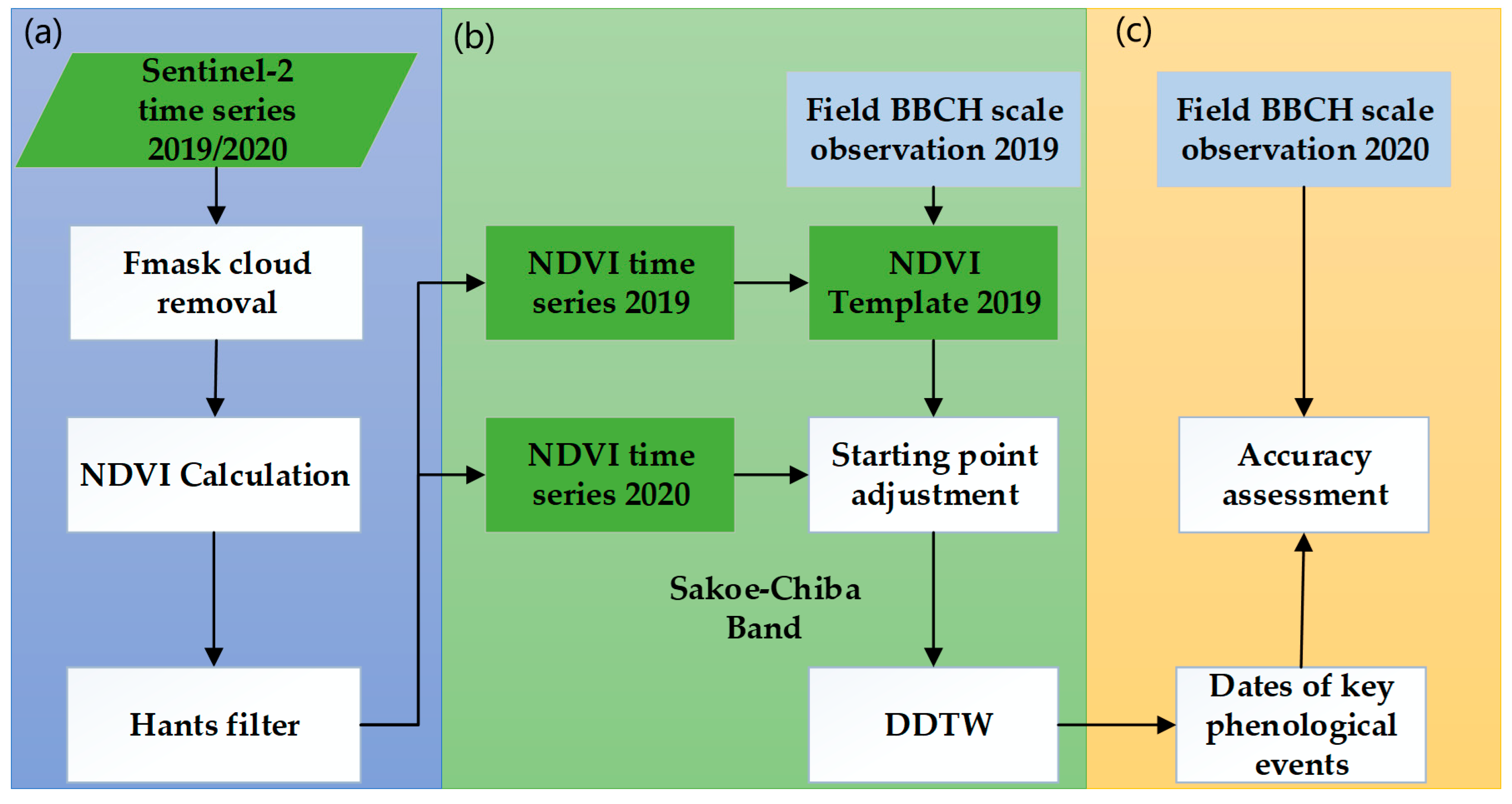
According to the Sentinel-2 NDVI time series data and the classification results of corn, the key phenological stages of corn were determined. The flow chart is shown in Figure 2 and mainly includes the following three steps: (a) data preprocessing; (b) phenology detection; (c) result generation and validation.

3.1. Overview of DDTW Principle

The Dynamic Time Warping (DTW) algorithm is a technique used for aligning and comparing two time series by calculating an optimal warping path between them. Given two sequences A (of length m) and B (of length n), a path matrix is created to store the pairwise distances between points. The algorithm enforces three constraints: (1) endpoint constraint, ensuring the path starts and ends at the first and last points of the matrix; (2) continuity constraint, allowing the path to advance one step at a time; and (3) monotonicity constraint, ensuring the path does not decrease. The cost function is calculated as shown in Equation (1) below
D i ,   j = 0 i f   i = j = 0 i f   i × j = 0   a n d   i j d q i , s j + m i n D i 1 ,   j 1 D i 1 ,   j D i ,   j 1 i f   i ,   j     1
where D i ,   j represents the accumulated distance between elements, q i and s j in sequences Q and S at positions i and j , respectively. The local distance between elements q i and s j in sequences Q and S is denoted by d q i , s j . The indices of the elements in sequences Q and S are represented by i and j , respectively.
Overall, the DTW algorithm includes two steps as shown in Figure 3. The optimal match between the two sequences is determined by the lowest distance path after alignment.
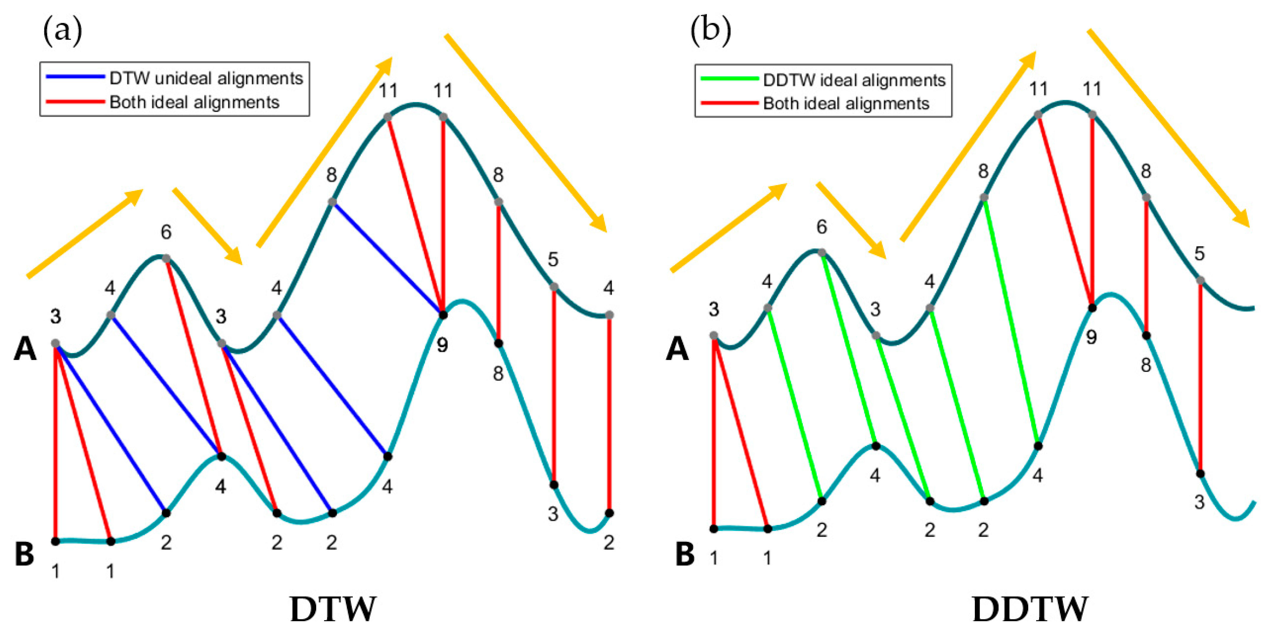
Although DTW is effectively used in numerous fields, it can sometimes yield pathological results due to its tendency to overcompensate for y-axis variations by distorting the x-axis. This method primarily focuses on the y-axis values of data points, which can lead to unexpected alignments. For instance, Figure 4a depicts an alignment result of DTW where curve A was shifted up by two units. The subsequent DTW alignment is represented by the unideal blue line in Figure 4a. The second data point in time series A, with a value of four, aligns with the fourth data point in series B, which also has a value of four; however, these points indicate differing trends. Specifically, in series A, this point signifies a rising trend, whereas in series B, the corresponding value marks a peak. Though DTW may deem the mapping between these points as perfect, it is intuitively more beneficial to steer clear of aligning differing trends.
To tackle this problem, we modified DTW [43] to consider not only the Y value of the data point but also its shape characteristics. Consequently, we altered the calculation of the cost matrix in DTW. The distance metric employed is not the Euclidean distance but rather the square of the difference between the estimated derivatives, referred to as DDTW. Assuming that the sequences to align are U and V in DDTW, the Equation for transforming the data point u i in sequence U is presented below [43]:
d i u = u i u i 1 + u i + 1 u i 1 / 2 2 , 1 < i < n ,
d d i , j = d i u d j v + min d d i 1 , j , d d i 1 , j 1 , d d i , j 1
where d i u represents the derivative of sequence U at position i ; u i , u i 1 , and u i + 1 are values of sequence U at different positions; n is the length of sequence U ; and d d i , j represents the distance between the transformed sequences at positions i and j .
As shown in Figure 4b, the DDTW algorithm shows greater robustness when handling the translation of time series A, ensuring aligned points share similar trends, indicating identical shape characteristics. This is particularly pertinent for phenology detection, where shape features often surpass a single NDVI value in importance.

3.2. Crop Phenology Determination

Crop phenology determination involves four steps: (1) establishment of phenological curve template, (2) time series starting point adjustment, (3) Sakoe–Chiba Band constraint, and (4) DDTW alignment and phenology determination, each of which will be introduced sequentially in the following sections.

3.2.1. Establishment of Phenological Curve Template

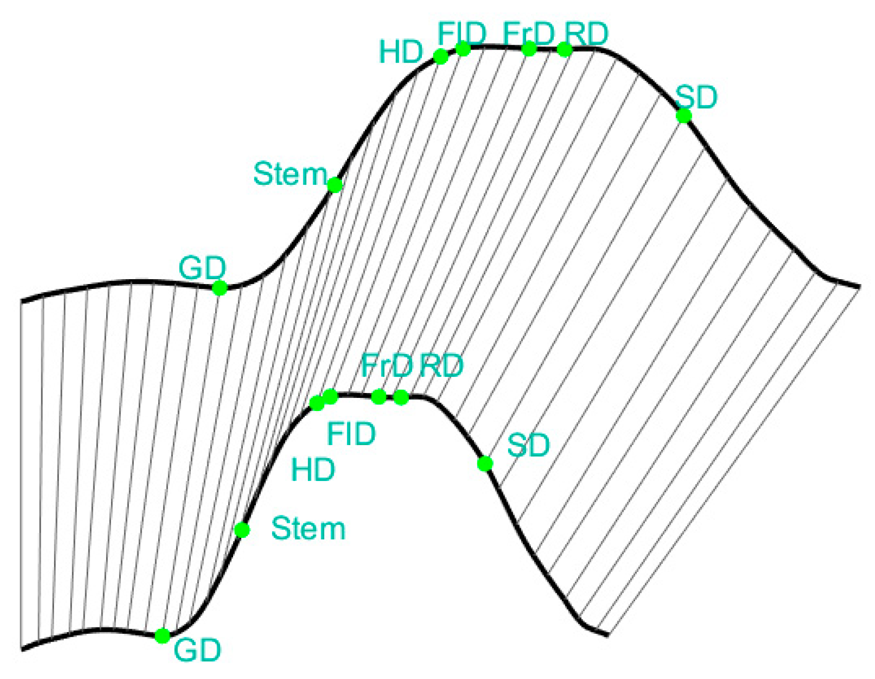
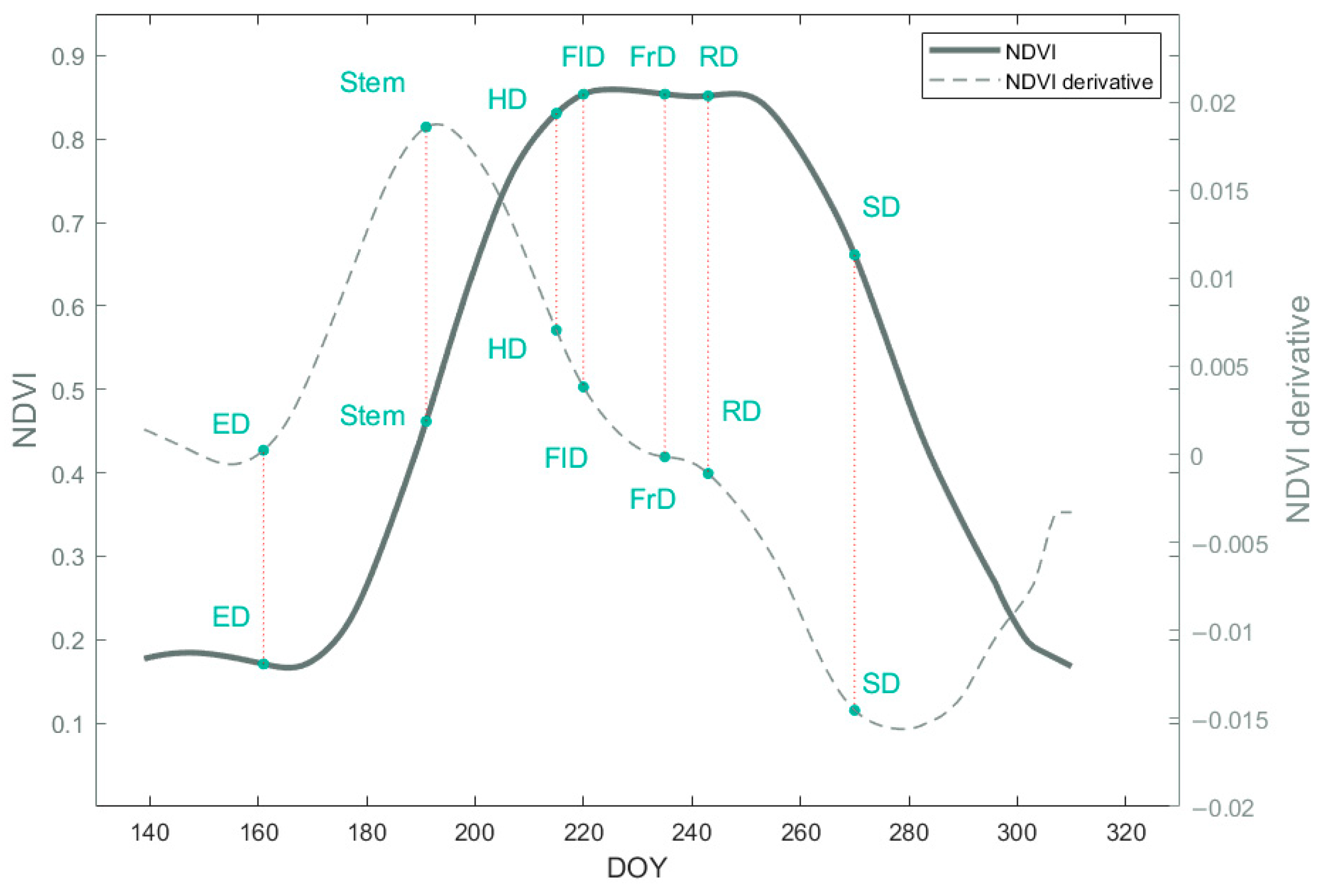
The accuracy of the phenological curve template directly influences the extraction accuracy of phenological information. We determined that the observation blocks based on ground observation data from 2019 and the Sentinel-2 NDVI data acquired under favorable atmospheric conditions in this area were used for the template curve establishment. We applied Hants function for filtering the NDVI time series and used interpolation to obtain a suitable NDVI temporal curve. Subsequently, we identified the phenological feature points on the template curve according to the ground observation data. We defined the following phenological feature points based on the BBCH standard on the template curve, including Emergence (ED), Stem elongation (Stem), heading (HD), Flowering (FlD), Development of Fruit (FrD), Ripening (RD), and Senescence (SD).
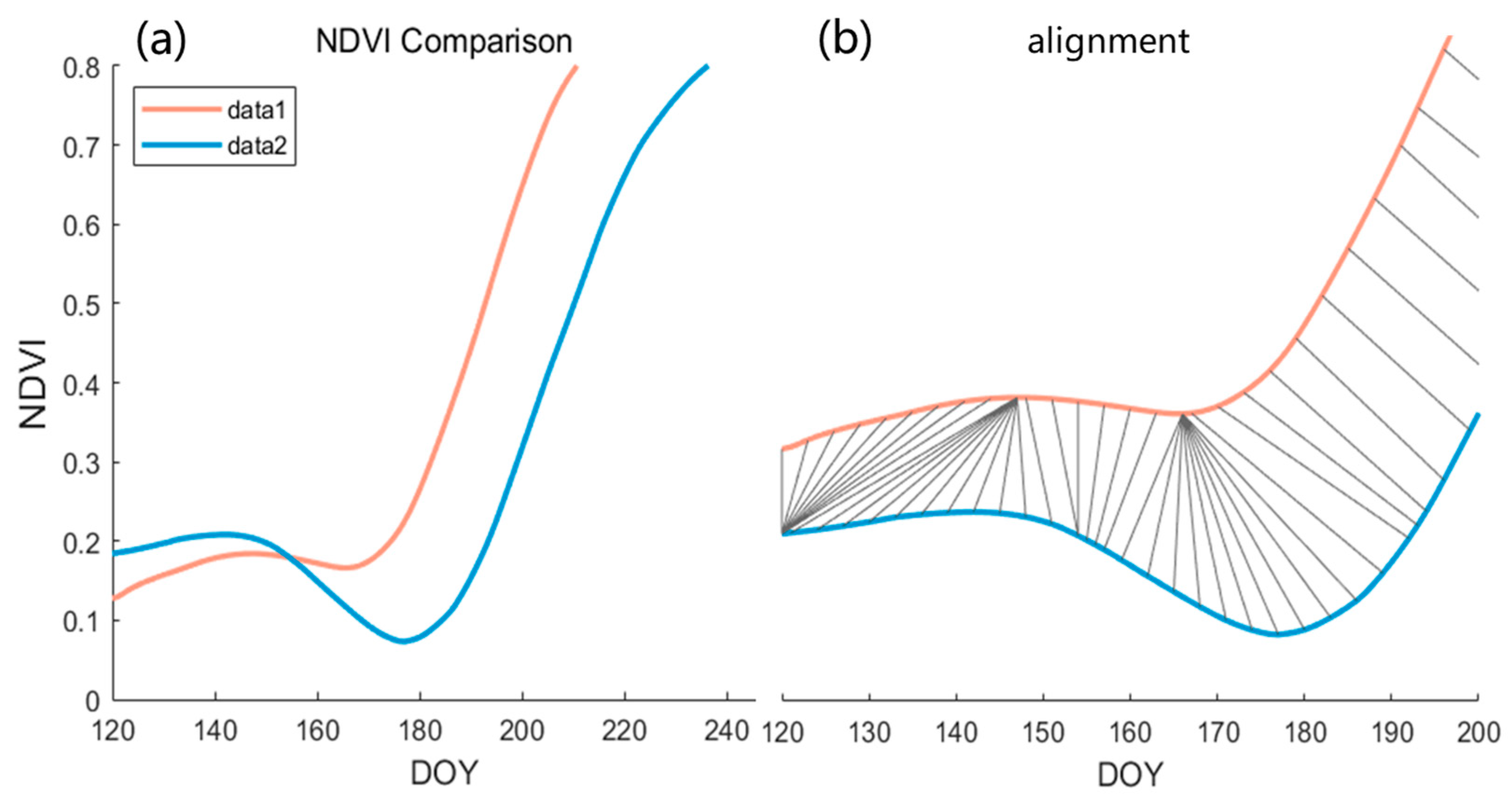
The growth of crops can be significantly impacted by various environmental factors, with cumulative temperature being one of the most influential. Suppose there is an inconsistency in the accumulated temperature across two planting years, this can easily lead to deformation of the NDVI time series curve along the x-axis (DOY). As demonstrated in Figure 5 below, the template is compressed to 0.7 times on the x-axis.
In Figure 5, the start of the growing season of the two NDVI curves deviates significantly. If we use the same phenological interval as the template, for instance, defining phenology based on a specific number of days from the starting point, it could lead to serious anomalies. However, the DDTW or DTW algorithm’s dynamic warping capability facilitates satisfactory alignment outcomes, even in the face of x-axis compression. This holds true even when these phenological intervals align with significant variations on the template. This is because the algorithm goes beyond merely aligning curve translations, and it dynamically adjusts alignment in accordance with the shape features of the target curve.

3.2.2. Time Series Starting Point Adjustment

Our satellite data collection often commences prior to the actual sowing and growth of crops. However, before the crops were planted, there were typically short NDVI peaks due to the weed growth. These NDVI variations present inconsistently across different NDVI time series and are usually irrelevant for subsequent alignment (Figure 6a). As depicted in Figure 6, the algorithm was able to manage the offset on the x-axis; however, challenges arose when other vegetation, such as weed, existed before the crops were planted. As illustrated in Figure 6b, despite the well-aligned stages of rapid vegetation growth, abnormal alignments were prevalent at the early stages. Owing to the global alignment attribute of the algorithm, failure to eliminate the time of soil and weed mixtures could potentially interfere with early phenology detection.
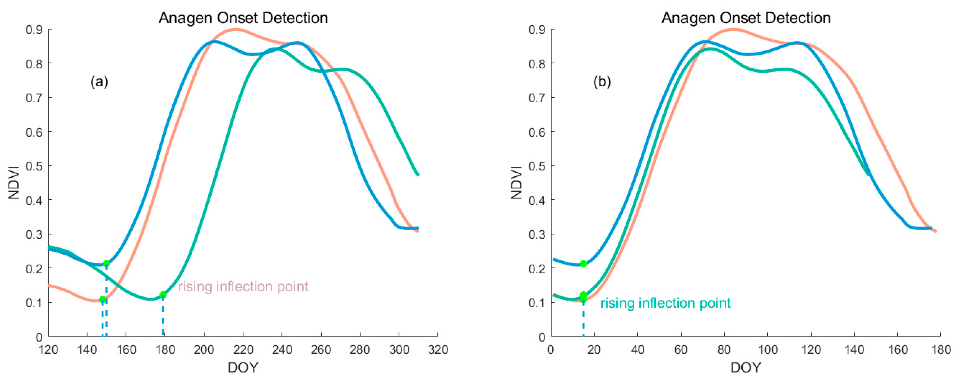
The initial NDVI time series begins from DOY 120. To minimize the influence of soil and weed before the growing season of corn on the NDVI time series alignment, we planned to adjust the starting point of the time series for both the template and target curves. The Emergence stage (ED) typically occurs within 10 days prior to the rising inflection point. Therefore, we adjust the starting point of the NDVI curve to be 15 days before the rising inflection point instead of DOY 120, and we proceed with subsequent operations. The detection condition for the rising inflection point was given by the following conditions (Equation (4)):
i = p p + 30 1 N D V I i + 1   >   N D V I i   >   25 N D V I r i s e _ e n d   >   0.6
where p represents the current corresponding NDVI data point; i represents the index of the NDVI data points within a 30-day window starting from point p ; N D V I i + 1 and N D V I i are the NDVI values at points i +1 and i , respectively; and r i s e _ e n d represents the end of the rising period.
The detection criteria for the rising inflection point are that the NDVI value after this point rises continuously for more than 25 days within 30 days. This condition is not strictly set to 30 days to reduce the influence of errors on the curve; it only requires that the overall curve shape after this point is rising. Another condition is that the peak value during the rising stage must be greater than 0.6, which is a relatively lenient requirement. The first point that meets these conditions is considered the rising inflection point.

3.2.3. Sakoe–Chiba Band Constraint

As discussed in Section 3.1, DTW can excessively distort the x-axis to account for y-axis variations, leading to the disproportionate correspondence of one point with the others. DTW is often combined with Sakoe–Chiba warped windows for various tasks, and many studies have demonstrated that Sakoe–Chiba Band constraints are very effective for improving accuracy [34,35,36,37], especially when processing time series that are not highly distorted. This is clearly illustrated in Figure 7, where two identical NDVI sequences (a) incur a downward shift in one sequence. This manipulation yields a corresponding cost matrix and path denoted in Figure 7b, resulting in an alignment outcome represented in Figure 7c. The implementation of a Sakoe–Chiba constraint involves assigning a value of infinity to elements outside a specified width near the main diagonal of the cost matrix (Figure 7e). This constraint ensures the backtracking path adheres closely to the main diagonal, limiting potential over-distortions (Figure 7f). To incorporate this constraint into the phenology extraction algorithm, one needs to set the value outside a specified width near the main diagonal of the cost matrix to infinity. This ensures that the backtracking path remains within the range of the main diagonal, preventing excessive distortion of the crop’s NDVI curve during alignment, which in turn facilitates accurate phenology extraction.
The Sakoe–Chiba Band constraint restricts the DTW backtracking algorithm’s path to a specific width along the diagonal, effectively limiting the maximum size of singularities but not entirely preventing their occurrence. The DDTW algorithm, with its emphasis on shape features, exhibits less sensitivity to y-axis shifts. However, DDTW combined with window constraints can also play an important role in avoiding excessive distortion of the curve. In real scenarios, numerous factors such as cloud interference and radiation distortion can affect the shape of the time series. Moreover, DDTW involves derivative calculations, which are inherently susceptible to noise. Importantly, implementing window constraints does not negatively impact original DDTW performance, often proving beneficial [34,35,36,37]. Applying window constraints can help mitigate this sensitivity, enhancing the algorithm’s performance, though the improvement is not as prominent as in traditional DTW. During the alignment of vegetation NDVI curves, having performed time series adjustment, the NDVI curve shapes at this stage should be similar, exhibiting only minor shifts along the time axis. Consequently, the Sakoe–Chiba Band constraint can be effectively applied, employing a typical window size of 20%.

3.2.4. DDTW Alignment and Phenology Determination

Adhering to the principle of DDTW warp alignment, we calculated the cost matrix and identified the backtracking path. The points on the path represent the best-aligned positions on the two curves, indicating the closest distance and most similar shape. Consequently, we can consider these points as corresponding to the same phenological stages. In other words, based on the reference phenology curve, we search for the point on the target curve closest to the characteristic phenology point on the reference phenology curve, and we consider this point as the phenology of the target curve. To find the phenological feature points corresponding to the target curve, we determined that when the feature point on the reference curve corresponds to a single point on the target curve, this point is also considered the phenological feature point of the target curve. When corresponding to multiple points, the mean value is taken as the target phenological feature point. Figure 8 demonstrates an example of how the DDTW algorithm was used to determine the phenological stage.
Assuming we only know three feature points (Features a, b, and c) on the reference trajectory (depicted in dark green), we sequentially identify the corresponding points (Features A, B, and C) on the target trajectory (light blue). In this context, three scenarios were examined: In Feature a, the mean value of the aligned points on the target trajectory is selected as Feature A for the target curve. In Feature b, only one point is aligned and directly chosen as Feature B. In Feature c, multiple points on the reference trajectory correspond to a single point on the target trajectory; however, Feature c on the reference curve still solely corresponds to a single point on the target trajectory, which is chosen as Feature C.

3.3. Crop Phenology Evaluation

The accuracy of the results was assessed by in situ observations in 2020, using three statistical measures to verify the accuracy: mean absolute error (MAE), root mean square error (RMSE), and Bias (e.g., Equations (5)–(7))
M A E = 1 n i = 1 n y i y i
R M S E = 1 n i = 1 n y i y i 2
B i a s = i = 1 n y i y i n
where n is the number of ground data detection, y i is the predicted phenological date, and y i is the actual phenological date.
To evaluate the detection capabilities of the DDTW method, we compared it with the two-step filtering (TSF) method [17]. The TSF method adopts a two-stage filtering approach that involves smoothing the VI time series and obtaining optimal scaling and shift parameters through a shape model fitting procedure. Following this, the dates of critical crop development stages are estimated using the initial values of the optimal scale parameters and shape models, which correspond to distinct phenological stages. These initial values are derived from in situ observations. To prove the effectiveness of the starting point adjustment, we also conducted the DTW experiment with and without the starting point adjustment. Lastly, we applied the proposed phenology detection framework to a larger area of corn fields, to visualize the temporal and spatial distribution of corn phenology.

4. Results

4.1. Establishment of Phenological Curve Template Results

We defined the following phenological feature points based on the BBCH standard on the template curve, including Emergence (ED), Stem elongation (Stem), Heading (HD), Flowering (FlD), Development of Fruit (FrD), Ripening (RD), and Senescence (SD), as illustrated in Figure 9 below:

4.2. Time Series Starting Point Adjustment Result

Figure 10 presents the process of adjusting the time series starting point. Accordingly, we adjusted the starting points of both the phenological curve template and the target time series.

4.3. Temporal and Spatial Distribution of Corn Phenology

For the corn fields in the area shown in the big black box in Figure 1, we employed the DDTW algorithm to extract seven key phenological stages during the growth of corn in 2020 and generated the phenological maps (Figure 11). In various phenology maps, we can observe the differences in color, indicating that the DOY to reach each phenological stage varies. For most corn fields, the Emergence day was between DOY 130 and 150. While for some fields, the Emergence day was between DOY 150 and 170.
Furthermore, there is a certain continuity on the map, suggesting that some areas and their surrounding regions experience similar phenological stages. Instances where the phenology of certain areas differs from their surrounding regions, such as the non-purple areas in the map of Emergence day, signify a later phenological stage—which is also reflected in the subsequent Stem elongation stage. This phenomenon is primarily related to the late sowing date. However, towards the end of the phenological cycle, these differences gradually diminish.
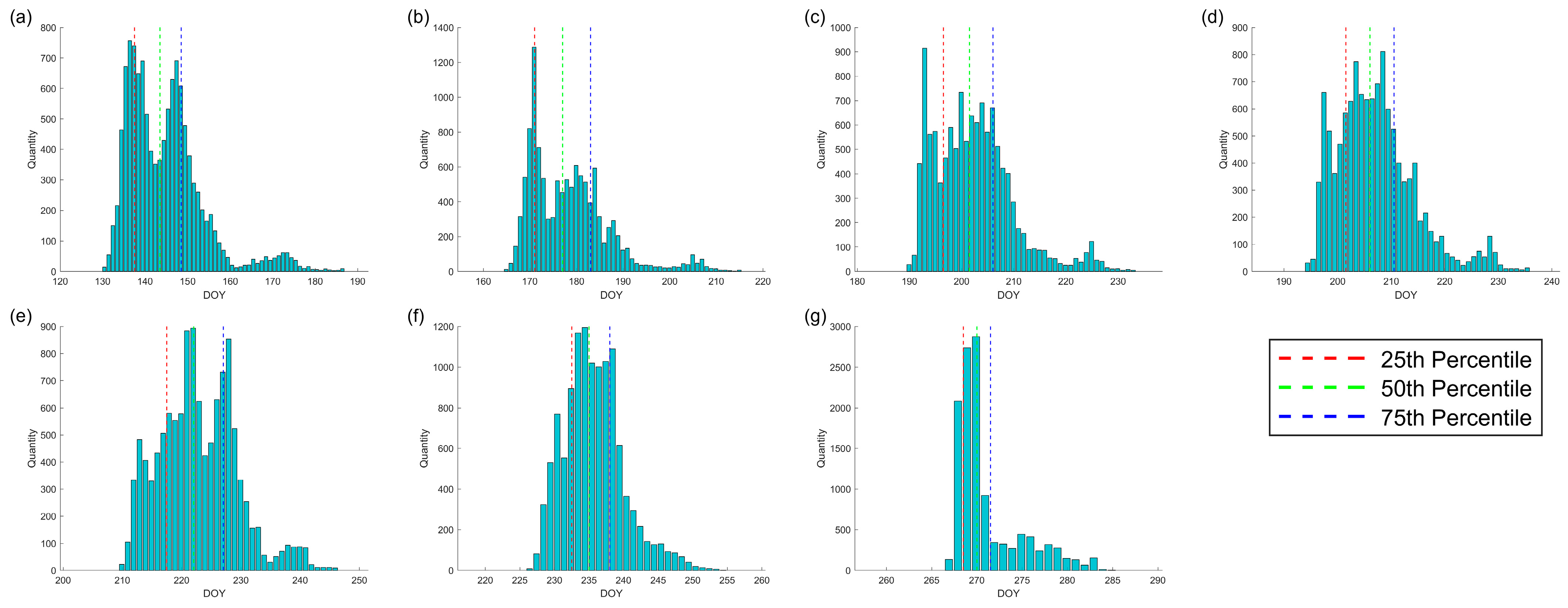
The frequency distributions corresponding to each phenological stage are illustrated in Figure 12. We observed that the Emergence stage (ED) primarily occurs between days 135 and 155, Stem elongation (Stem) is concentrated between days 170 and 190, Heading (HD) typically takes place between days 195 and 210, Flowering (FlD) is predominantly found between days 195 and 215, Development of Fruit (FrD) mainly occurs between days 215 and 230, Ripening (RD) is focused between days 230 and 240, and Senescence (SD) primarily happens between days 265 and 270. The Emergence date exhibits two distinct minor peaks on the frequency graph, which may result from varying sowing dates. For Stem elongation, the bimodal distribution of the histogram is quite noticeable, likely due to the differences in seeding time. However, during the mid-growth stage, Flowering (FlD), Development of Fruit (FrD), and Ripening (RD) exhibit a more concentrated histogram as the phenological interval between early- and later-planted corn decreases, owing to improved thermal conditions and faster growth of the later-sown crop. With continuous growth and upon reaching the late growth stage, the Senescence date becomes relatively close, regardless of whether the corn was planted earlier or later. This may be due to temperature or other factors (such as harvesting), resulting in a more concentrated histogram as the corn matures and begins to senesce.

4.4. Accuracy of the DDTW Phenology Detection for Corn

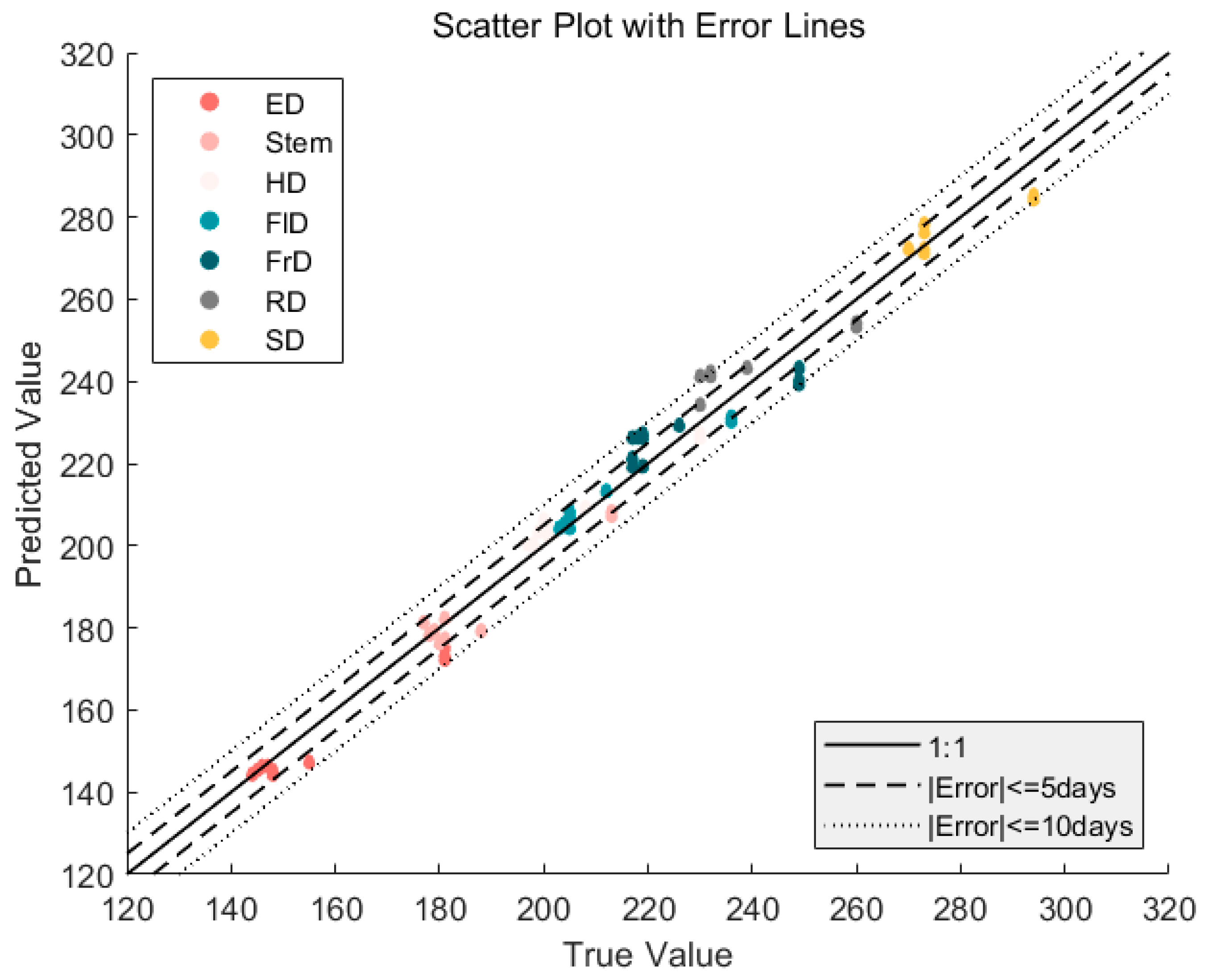
Table 3 shows the extraction results of the phenology stages, tested by the 2020 ground observation data. For phenology stages with distinct shape characteristics, such as Stem elongation and Heading, the RMSE, MAE, and bias are all less than 5 days. However, for phenology stages with less distinct shapes, such as Development of Fruit and Ripening, the RMSE can still be within 10 days. It is evident that due to the inconspicuous characteristics of these phenological stages, the detection is difficult and deviation is larger. In general, using the DDTW method to extract phenological stages yields high accuracy. As shown in Figure 13, the results of the phenological stages extracted by DDTW were verified. It performs well for phenological features with obvious characteristics and demonstrates good detection ability for inconspicuous features.
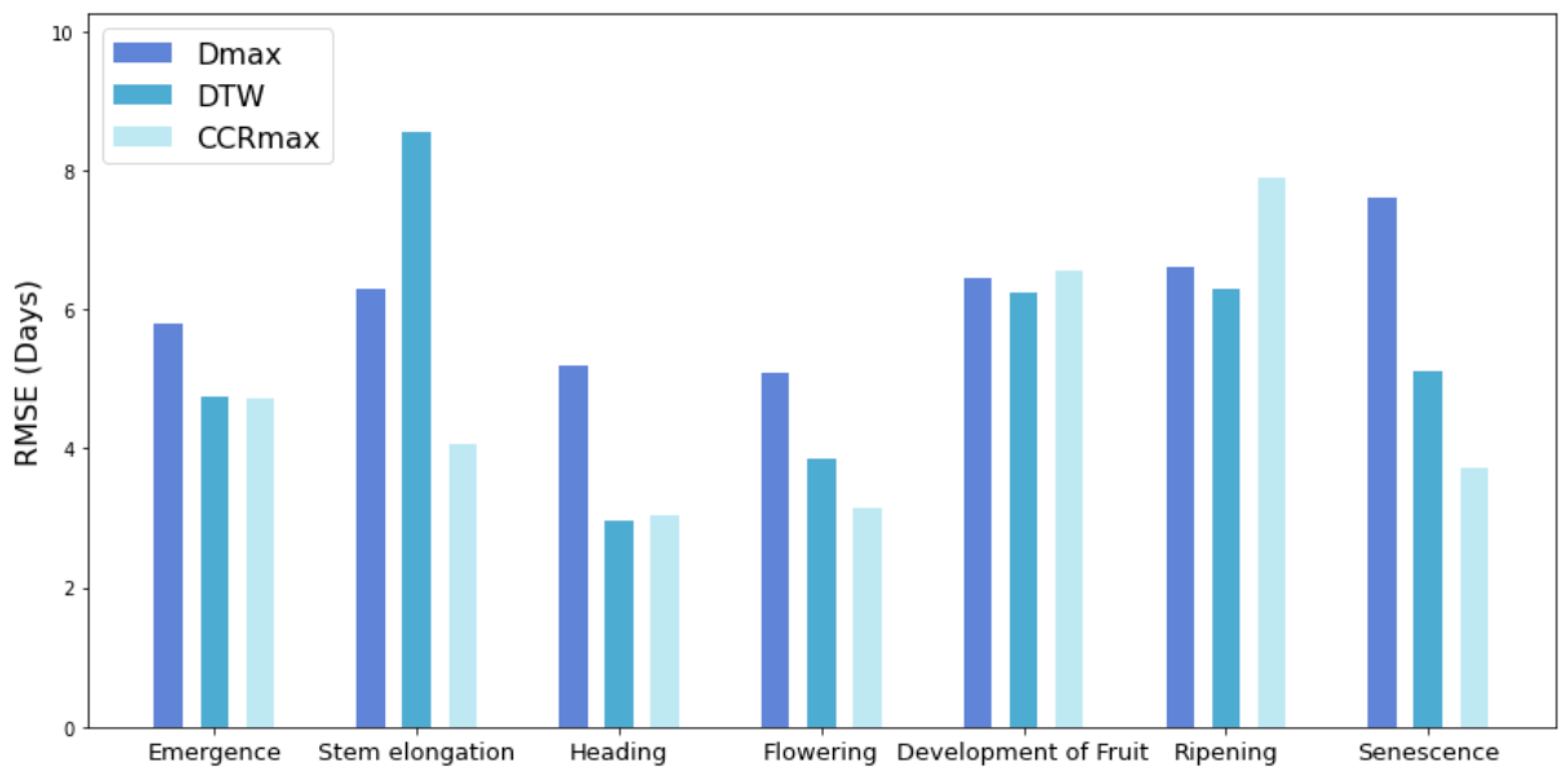
We compared the phenology extraction results using the DDTW algorithm with the TSF and DTW. As illustrated in Figure 14, the DDTW algorithm demonstrates an obvious advantage in extraction accuracy compared to other methods for most stages. For the Development of Fruit and Ripening stages, the performance of the DDTW is inferior to the other two methods. A plausible explanation is that these two stages are often found in areas with high NDVI values. However, due to observation errors or noise, there might be subtle differences in the derivative curves of vegetation, which can be erroneously identified as “incorrect” features. In comparison, other algorithms are slightly more stable, as the derivative is more sensitive to noise. DTW and DDTW offer significant advantages over TSF at the Senescence stage. TSF allows for basic translation of all points along a curve, depending on the shift and scaling parameters, while DDTW provides the flexibility to distort the curve. This adaptability enables it to account for variations in time and growth speed and to adjust the data in more accurate and robust alignments. The DDTW outperforms the DTW and TSF at most stages, suggesting that it is more effective at capturing and reflecting the shape features of time series data. By considering the derivative information, DDTW is better suited to handle variations in the shape of the curves.
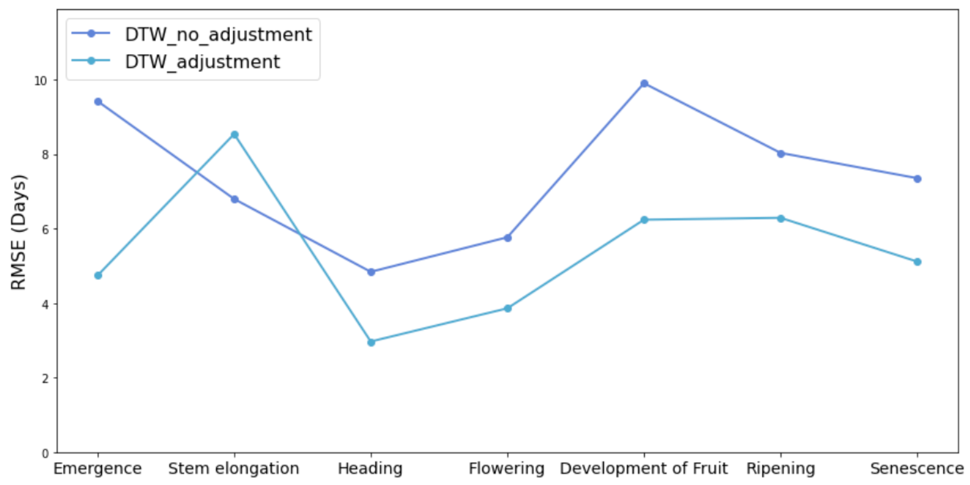
Within the same window constraints, we compared the DTW experiment results with and without the time series starting point adjustment, as illustrated in Figure 15. We found that the algorithm performance was improved after adjusting the starting point, particularly at the Emergence stage. This improvement could be attributed to the reduction in interference from the early stage before the emergence of crops.

5. Discussion

5.1. Contributions and Advantages of the Study

In this study, we proposed a DDTW-based phenology detection framework for the estimation of corn phenological stages based on the BBCH scale. This method allows the construction of the Sentinel-2 NDVI time series template acquired in previous years with the defined phenological events from ground measurements, matching it with unknown NDVI time series. Subsequently, phenological stages for other years can be identified.
The framework integrated the time series starting point adjustment and Sakoe–Chiba Band constraints with the DDTW to increase the accuracy of phenology detection. By comparing the DTW results with and without the time series starting point adjustment, we found that the algorithm performance was improved after adjusting the starting point. At the early stage before the corn growing season, complex factors such as weed growth and seeding events may cause the high fluctuation of NDVI values. By detecting and adjusting the starting point, the interference of the NDVI data at the early stage was removed, and it is beneficial to detect corn phenological stages. After adjusting the starting date, the NDVI curve did not deviate significantly on the time axis. We also employed the Sakoe–Chiba Band constraint, a common constraint in DTW and related algorithms, to avoid excessive distortion of the curve. The Sakoe–Chiba Band constraint effectively suppresses extreme one-to-many situations, especially on curves with relatively large noise, thus enhancing the overall performance of the phenological detection process.
In our comparative analysis of the DTW and DDTW algorithms, we observed that DDTW excels beyond the performance of the DTW algorithm. An aspect of DDTW’s potential is its ability to consider the shape characteristics of the NDVI curve, rather than solely focusing on the NDVI values. This yields a more robust and precise performance in phenological detection. Even under extreme weather conditions, our DDTW-based method consistently performs effectively. Whereas lower NDVI values caused by drought or frost might severely disrupt the DTW, leading to significant curve distortion, DDTW maintains its ability to identify phenological stages as long as the overall trend or shape of the NDVI does not dramatically change.
The TSF’s presumption of synchronized phenological stages often lacks accuracy when confronted with disparate growth rates and asynchronous shifts triggered by fluctuating weather conditions, thereby reducing its precision in phenology detection. TSF allows for the basic translation of every point along a curve, contingent on the shift and scaling parameters, while DDTW proffers the flexibility to distort the curve. This flexibility enables it to account for variations in time and growth speed and to adjust the data in more accurate and robust alignments.

5.2. Limitations of the Proposed Method and Outlooks

It is evident that utilizing DDTW for alignment may not be sufficient to improve the extraction accuracy in phenological stages with weak shape information, such as Development of Fruit and Ripening. Additionally, the Vegetation Index NDVI is prone to oversaturation, which can further hinder the accuracy of the extraction process.
To improve phenology detection accuracy, it could be advantageous to explore alternative vegetation indices less susceptible to oversaturation, such as the Enhanced Vegetation Index (EVI or EVI2) [49,50]. These indices are specifically designed to address some NDVI limitations and could potentially offer more precise phenological information.
Furthermore, incorporating both the value and the derivative of data points in the DTW warp alignment process might be beneficial. This can be achieved by employing a hybrid approach that combines the strengths of both DTW and DDTW, allowing for a more comprehensive assessment of time series similarities. By considering both the value and the derivative, this approach could potentially improve the detection of weakly characterized phenological stages, leading to enhanced overall accuracy in phenological analysis.
To apply this method to different regions or crop types, it is essential to establish a template curve that aligns with the local crops, necessitating certain ground observations. The precision of these observations directly influences phenology detection accuracy; however, acquiring high-quality time series satellite observations over croplands can be challenging due to frequent cloud contaminations over extended periods of time [51,52]. This issue can be mitigated by merging high-temporal resolution observations with high-spatial resolution ones, such as HLS-MODIS, HLS-VIIRS, HLS-ABI, etc. Furthermore, creating the crop template requires consistent, long-term ground observations, which may not always be feasible in extensive geographical regions. Compared to other algorithms determining phenology events based on curve characteristics, this study’s method has its limitations.

6. Conclusions

In conclusion, this study introduced a novel DDTW framework for detecting corn phenology based on Sentinel-2 NDVI time series data. The proposed framework effectively integrates the DTW-based algorithm with the BBCH-scale model, which is suitable for corn and can also be extended to other crops. This framework achieved full phenology detection of corn based on the BBCH scale. It also outperformed other methods such as DTW and TSF at most phenological stages, and the RMSEs were less than 5 days at these stages.
The phenology extraction method proposed in this study can provide valuable support for crop field management and policy development. In the future, our intention is to explore the potential of this method for near real-time detection of phenological events. By conducting experiments and validating our approach with real-time data, we hope to contribute to a more sustainable and productive agriculture.

Author Contributions

Conceptualization, J.Y.; methodology, J.Y. and C.L.; formal analysis, H.H., W.B. and D.C.; investigation, C.L.; data curation, W.B., H.H. and D.C.; writing—original draft preparation, J.Y. and W.B.; writing—review and editing, C.L. All authors have read and agreed to the published version of the manuscript.

Funding

This research was funded by the National Nature Science Foundation of China, grant number 42101352.

Data Availability Statement

The data of this study are available upon reasonable request.

Acknowledgments

The authors acknowledge the Europe Space Agency (ESA) for providing the Sentinel-2 data and the Agriculture and Agri-Food Canada (AAFC) for providing the Annual Crop Inventory (ACI) data. The authors appreciate the assistance of the GITA lab at the University of Western Ontario for collecting field data. The authors sincerely thank all the anonymous reviewers for their valuable comments and suggestions.

Conflicts of Interest

The authors declare no conflict of interest.

References

  1. Myneni, R.B.; Keeling, C.D.; Tucker, C.J.; Asrar, G.; Nemani, R.R. Increased Plant Growth in the Northern High Latitudes from 1981 to 1991. Nature 1997, 386, 698–702. [Google Scholar] [CrossRef]
  2. Schwartz, M.D.; Reed, B.C. Surface Phenology and Satellite Sensor-Derived Onset of Greenness: An Initial Comparison. Int. J. Remote Sens. 1999, 20, 3451–3457. [Google Scholar] [CrossRef]
  3. White, M.A.; Thornton, P.E.; Running, S.W. A Continental Phenology Model for Monitoring Vegetation Responses to Interannual Climatic Variability. Glob. Biogeochem. Cycles 1997, 11, 217–234. [Google Scholar] [CrossRef]
  4. Gao, F.; Zhang, X. Mapping Crop Phenology in near Real-Time Using Satellite Remote Sensing: Challenges and Opportunities. J. Remote Sens. 2021, 2021, 8379391. [Google Scholar] [CrossRef]
  5. Anderson, M.C.; Hain, C.R.; Jurecka, F.; Trnka, M.; Hlavinka, P.; Dulaney, W.; Otkin, J.A.; Johnson, D.; Gao, F. Relationships between the Evaporative Stress Index and Winter Wheat and Spring Barley Yield Anomalies in the Czech Republic. Clim. Res. 2016, 70, 215–230. [Google Scholar] [CrossRef] [Green Version]
  6. Walthall, C.; Anderson, C.; Takle, E.; Baumgard, L.; Wright-Morton, L. Climate Change and Agriculture in the United States: Effects and Adaptation; Adventure Scientists: Bozeman, MT, USA, 2013. [Google Scholar]
  7. Anderson, M.C.; Zolin, C.A.; Sentelhas, P.C.; Hain, C.R.; Tetrault, R. The Evaporative Stress Index as an Indicator of Agricultural Drought in Brazil: An Assessment Based on Crop Yield Impacts. Remote Sens. Environ. 2016, 174, 82–99. [Google Scholar] [CrossRef]
  8. Yang, Y.; Anderson, M.C.; Gao, F.; Wardlow, B.; Hain, C.R.; Otkin, J.A.; Alfieri, J.; Yang, Y.; Sun, L.; Dulaney, W. Field-Scale Mapping of Evaporative Stress Indicators of Crop Yield: An Application over Mead, NE, USA. Remote Sens. Environ. 2018, 210, 387–402. [Google Scholar] [CrossRef]
  9. Zeng, L.; Wardlow, B.D.; Xiang, D.; Hu, S.; Li, D. A Review of Vegetation Phenological Metrics Extraction Using Time-Series, Multispectral Satellite Data. Remote Sens. Environ. 2020, 237, 111511. [Google Scholar] [CrossRef]
  10. Asner, G.P.; Townsend, A.R.; Braswell, B.H. Satellite Observation of El Nino Effects on Amazon Forest Phenology and Productivity. Geophys. Res. Lett. 2000, 27, 981–984. [Google Scholar] [CrossRef] [Green Version]
  11. Knudby, A. An AVHRR-Based Model of Groundnut Yields in the Peanut Basin of Senegal. Int. J. Remote Sens. 2004, 25, 3161–3175. [Google Scholar] [CrossRef]
  12. Paruelo, J.M.; Epstein, H.E.; Lauenroth, W.K.; Burke, I.C. ANPP Estimates from NDVI for the Central Grassland Region of the United States. Ecology 1997, 78, 953–958. [Google Scholar] [CrossRef]
  13. Roetzer, T.; Wittenzeller, M.; Haeckel, H.; Nekovar, J. Phenology in Central Europe—Differences and Trends of Spring Phenophases in Urban and Rural Areas. Int. J. Biometeorol. 2000, 44, 60–66. [Google Scholar] [CrossRef] [PubMed]
  14. Tucker, C.J.; Fung, I.Y.; Keeling, C.D.; Gammon, R.H. Relationship between Atmospheric CO2 Variations and a Satellite-Derived Vegetation Index. Nature 1986, 319, 195–199. [Google Scholar] [CrossRef]
  15. Zhang, X.; Friedl, M.A.; Schaaf, C.B.; Strahler, A.H.; Hodges, J.C.F.; Gao, F.; Reed, B.C.; Huete, A. Monitoring vegetation phenology using MODIS. Remote Sens. Environ. 2003, 84, 471–475. [Google Scholar] [CrossRef]
  16. Liao, C.; Wang, J.; Shan, B.; Shang, J.; Dong, T.; He, Y. Near Real-Time Detection and Forecasting of within-Field Phenology of Winter Wheat and Corn Using Sentinel-2 Time-Series Data. ISPRS J. Photogramm. Remote Sens. 2023, 196, 105–119. [Google Scholar] [CrossRef]
  17. Sakamoto, T.; Wardlow, B.D.; Gitelson, A.A.; Verma, S.B.; Suyker, A.E.; Arkebauer, T.J. A Two-Step Filtering Approach for Detecting Maize and Soybean Phenology with Time-Series MODIS Data. Remote Sens. Environ. 2010, 114, 2146–2159. [Google Scholar] [CrossRef]
  18. Gan, L.; Cao, X.; Chen, X.; Dong, Q.; Cui, X.; Chen, J. Comparison of MODIS-Based Vegetation Indices and Methods for Winter Wheat Green-up Date Detection in Huanghuai Region of China. Agric. For. Meteorol. 2020, 288, 108019. [Google Scholar] [CrossRef]
  19. Vrieling, A.; Skidmore, A.K.; Wang, T.; Meroni, M.; Ens, B.J.; Oosterbeek, K.; O’Connor, B.; Darvishzadeh, R.; Heurich, M.; Shepherd, A. Spatially Detailed Retrievals of Spring Phenology from Single-Season High-Resolution Image Time Series. Int. J. Appl. Earth Obs. Geoinf. 2017, 59, 19–30. [Google Scholar] [CrossRef]
  20. Zhang, X.; Friedl, M.A.; Schaaf, C.B. Sensitivity of Vegetation Phenology Detection to the Temporal Resolution of Satellite Data. Int. J. Remote Sens. 2009, 30, 2061–2074. [Google Scholar] [CrossRef]
  21. Sakamoto, T. Refined Shape Model Fitting Methods for Detecting Various Types of Phenological Information on Major US Crops. ISPRS J. Photogramm. Remote Sens. 2018, 138, 176–192. [Google Scholar] [CrossRef]
  22. Shen, Y.; Zhang, X.; Yang, Z. Mapping Corn and Soybean Phenometrics at Field Scales over the United States Corn Belt by Fusing Time Series of Landsat 8 and Sentinel-2 Data with VIIRS Data. ISPRS J. Photogramm. Remote Sens. 2022, 186, 55–69. [Google Scholar] [CrossRef]
  23. Liu, L.; Cao, R.; Chen, J.; Shen, M.; Wang, S.; Zhou, J.; He, B. Detecting Crop Phenology from Vegetation Index Time-Series Data by Improved Shape Model Fitting in Each Phenological Stage. Remote Sens. Environ. 2022, 277, 113060. [Google Scholar] [CrossRef]
  24. Petitjean, F.; Ketterlin, A.; Gançarski, P. A Global Averaging Method for Dynamic Time Warping, with Applications to Clustering. Pattern Recognit. 2011, 44, 678–693. [Google Scholar] [CrossRef]
  25. Petitjean, F.; Inglada, J.; Gançarski, P. Satellite Image Time Series Analysis under Time Warping. IEEE Trans. Geosci. Remote Sens. 2012, 50, 3081–3095. [Google Scholar] [CrossRef]
  26. Romani, L.A.; Goncalves, R.R.V.; Zullo, J.; Traina, C.; Traina, A.J. New DTW-Based Method to Similarity Search in Sugar Cane Regions Represented by Climate and Remote Sensing Time Series. In Proceedings of the 2010 IEEE International Geoscience and Remote Sensing Symposium, Honolulu, HI, USA, 25–30 July 2010; pp. 355–358. [Google Scholar]
  27. Sakoe, H.; Chiba, S. Dynamic Programming Algorithm Optimization for Spoken Word Recognition. IEEE Trans. Acoust. Speech Signal Process. 1978, 26, 43–49. [Google Scholar] [CrossRef] [Green Version]
  28. Belgiu, M.; Csillik, O. Sentinel-2 Cropland Mapping Using Pixel-Based and Object-Based Time-Weighted Dynamic Time Warping Analysis. Remote Sens. Environ. 2018, 204, 509–523. [Google Scholar] [CrossRef]
  29. Csillik, O.; Belgiu, M.; Asner, G.P.; Kelly, M. Object-Based Time-Constrained Dynamic Time Warping Classification of Crops Using Sentinel-2. Remote Sens. 2019, 11, 1257. [Google Scholar] [CrossRef] [Green Version]
  30. Guan, X.; Liu, G.; Huang, C.; Meng, X.; Liu, Q.; Wu, C.; Ablat, X.; Chen, Z.; Wang, Q. An Open-Boundary Locally Weighted Dynamic Time Warping Method for Cropland Mapping. ISPRS Int. J. Geo-Inf. 2018, 7, 75. [Google Scholar] [CrossRef] [Green Version]
  31. Maus, V.; Câmara, G.; Cartaxo, R.; Sanchez, A.; Ramos, F.M.; De Queiroz, G.R. A Time-Weighted Dynamic Time Warping Method for Land-Use and Land-Cover Mapping. IEEE J. Sel. Top. Appl. Earth Obs. Remote Sens. 2016, 9, 3729–3739. [Google Scholar] [CrossRef]
  32. Baumann, M.; Ozdogan, M.; Richardson, A.D.; Radeloff, V.C. Phenology from Landsat When Data Is Scarce: Using MODIS and Dynamic Time-Warping to Combine Multi-Year Landsat Imagery to Derive Annual Phenology Curves. Int. J. Appl. Earth Obs. Geoinf. 2017, 54, 72–83. [Google Scholar] [CrossRef]
  33. Huseby, R.B.; Aurdal, L.; Eikvil, L.; Solberg, R.; Vikhamar, D.; Solberg, A. Alignment of Growth Seasons from Satellite Data. In Proceedings of the International Workshop on the Analysis of Multi-Temporal Remote Sensing Images, Biloxi, MS, USA, 16–18 May 2005; pp. 213–216. [Google Scholar]
  34. Geler, Z. Role of Similarity Measures in Time Series Analysis. Ph.D. Thesis, University of Novi Sad (Serbia), Novi Sad, Serbia, 2015. [Google Scholar]
  35. Geler, Z.; Kurbalija, V.; Radovanović, M.; Ivanović, M. Impact of the Sakoe-Chiba Band on the DTW Time Series Distance Measure for k NN Classification. In Proceedings of the Knowledge Science, Engineering and Management: 7th International Conference, KSEM 2014, Sibiu, Romania, 16–18 October 2014; pp. 105–114. [Google Scholar]
  36. Kurbalija, V.; Radovanović, M.; Geler, Z.; Ivanović, M. The Influence of Global Constraints on DTW and LCS Similarity Measures for Time-Series Databases. In the Third International Conference on Software, Services and Semantic Technologies S3T 2011; Springer: Berlin/Heidelberg, Germany, 2011; pp. 67–74. [Google Scholar]
  37. Kurbalija, V.; Radovanović, M.; Geler, Z.; Ivanović, M. The Influence of Global Constraints on Similarity Measures for Time-Series Databases. Knowl. Based Syst. 2014, 56, 49–67. [Google Scholar] [CrossRef] [Green Version]
  38. Cheng, K.; Wang, J. Forest-Type Classification Using Time-Weighted Dynamic Time Warping Analysis in Mountain Areas: A Case Study in Southern China. Multidiscip. Digit. Publ. Inst. 2019, 10, 1040. [Google Scholar] [CrossRef] [Green Version]
  39. Zhao, F.; Yang, G.; Yang, X.; Cen, H.; Zhu, Y.; Han, S.; Yang, H.; He, Y.; Zhao, C. Determination of Key Phenological Phases of Winter Wheat Based on the Time-Weighted Dynamic Time Warping Algorithm and MODIS Time-Series Data. Remote Sens. 2021, 13, 1836. [Google Scholar] [CrossRef]
  40. Kumar, V.; Grossman, R. Derivative Dynamic Time Warping. In Proceedings of the 2001 SIAM International Conference on Data Mining; SIAM: Philadelphia, PA, USA, 2011. [Google Scholar]
  41. Rath, T.M.; Manmatha, R. Word Image Matching Using Dynamic Time Warping. In Proceedings of the 2003 IEEE Computer Society Conference on Computer Vision and Pattern Recognition, Madison, WI, USA, 18–20 June 2003; Volume 2, p. II. [Google Scholar]
  42. Ventura, F.; Marletto, V.; Traini, S.; Tomei, F.; Botarelli, L.; Rossi, P. Validation of Development Models for Winter Cereals and Maize with Independent Agrophenological Observations in the BBCH Scale. Riv. Ital. Di Agrometeorol. 2009, 14, 17–26. [Google Scholar]
  43. Hird, J.N.; McDermid, G.J. Noise Reduction of NDVI Time Series: An Empirical Comparison of Selected Techniques. Remote Sens. Environ. 2009, 113, 248–258. [Google Scholar] [CrossRef]
  44. Qiu, S.; Zhu, Z.; He, B. Fmask 4.0: Improved Cloud and Cloud Shadow Detection in Landsats 4–8 and Sentinel-2 Imagery. Remote Sens. Environ. 2019, 231, 111205. [Google Scholar] [CrossRef]
  45. Navarro, A.; Rolim, J.; Miguel, I.; Catalão, J.; Silva, J.; Painho, M.; Vekerdy, Z. Crop Monitoring Based on SPOT-5 Take-5 and Sentinel-1A Data for the Estimation of Crop Water Requirements. Remote Sens. 2016, 8, 525. [Google Scholar] [CrossRef] [Green Version]
  46. Rouse, J.W.; Haas, R.H.; Schell, J.A.; Deering, D.W. Monitoring Vegetation Systems in the Great Plains with ERTS. NASA Spec. Publ. 1974, 351, 309. [Google Scholar]
  47. Ahn, B. Agriculture and Agri-Food Canada (AAFC). Available online: https://agriculture.canada.ca/en (accessed on 6 July 2023).
  48. Hess, M.; Barralis, G.; Bleiholder, H.; Buhr, L.; Eggers, T.H.; Hack, H.; Stauss, R. Use of the Extended BBCH Scale—General for the Descriptions of the Growth Stages of Mono; and Dicotyledonous Weed Species. Weed Res. 1997, 37, 433–441. [Google Scholar] [CrossRef]
  49. Jiang, Z.; Huete, A.R.; Didan, K.; Miura, T. Development of a Two-Band Enhanced Vegetation Index without a Blue Band. Remote Sens. Environ. 2008, 112, 3833–3845. [Google Scholar] [CrossRef]
  50. Matsushita, B.; Yang, W.; Chen, J.; Onda, Y.; Qiu, G. Sensitivity of the Enhanced Vegetation Index (EVI) and Normalized Difference Vegetation Index (NDVI) to Topographic Effects: A Case Study in High-Density Cypress Forest. Sensors 2007, 7, 2636–2651. [Google Scholar] [CrossRef] [PubMed] [Green Version]
  51. Prudente, V.H.R.; Martins, V.S.; Vieira, D.C.; de Silva, N.R.F.E.; Adami, M.; Sanches, I.D. Limitations of Cloud Cover for Optical Remote Sensing of Agricultural Areas across South America. Remote Sens. Appl. Soc. Environ. 2020, 20, 100414. [Google Scholar] [CrossRef]
  52. Whitcraft, A.K.; Vermote, E.F.; Becker-Reshef, I.; Justice, C.O. Cloud Cover throughout the Agricultural Growing Season: Impacts on Passive Optical Earth Observations. Remote Sens. Environ. 2015, 156, 438–447. [Google Scholar] [CrossRef]
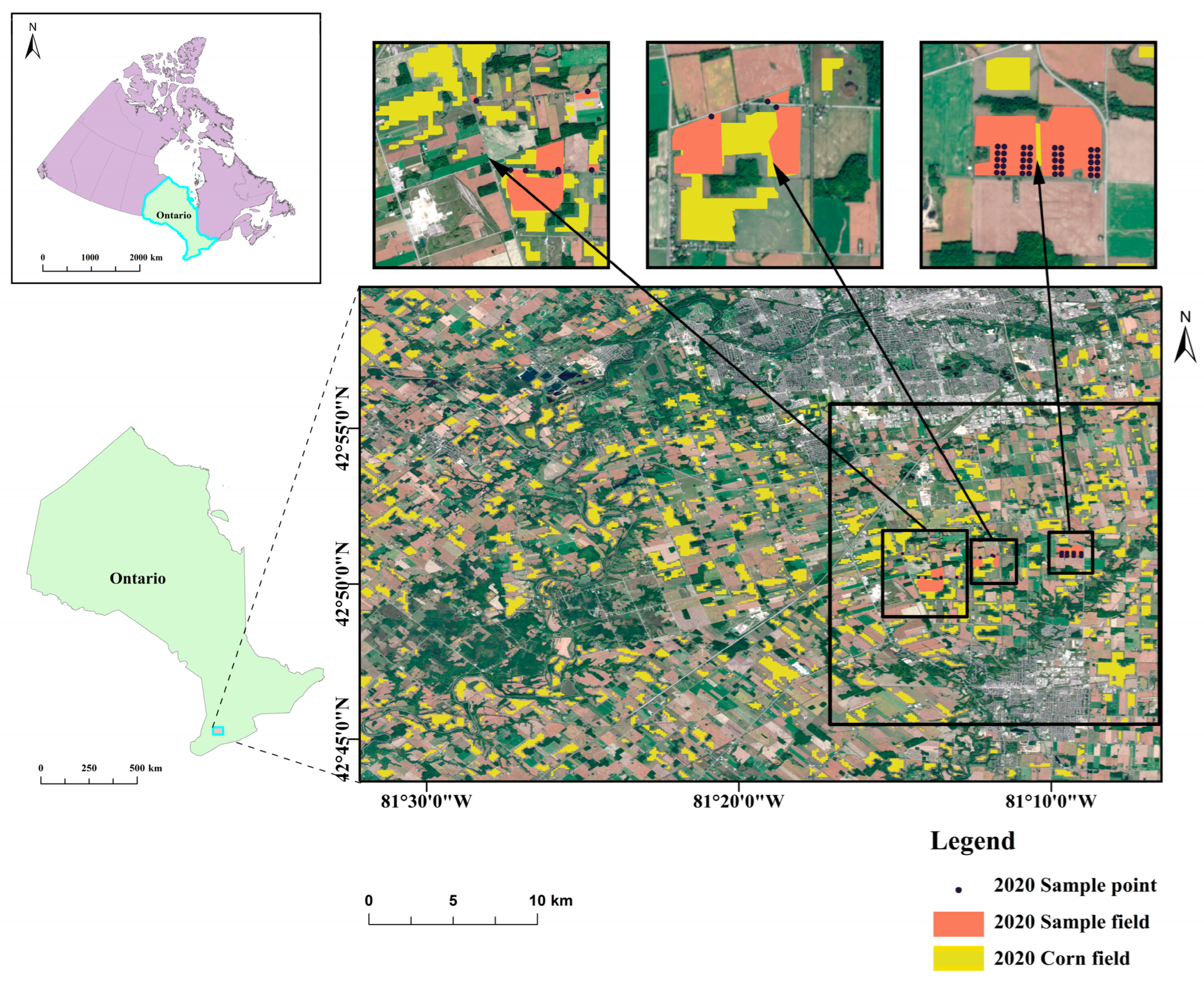
Figure 1. Location of the study site; RGB image of the Sentinel-2 data acquired in September; and the spatial distribution of corn, sample fields, and sample points surveyed in 2020 shown in the black boxes.
Remotesensing 15 03456 g001
Figure 2. Workflow of a Derivative Dynamic Time Warping (DDTW) method for determining corn phenology. (a) Data preprocessing; (b) phenology detection; (c) result generation and validation.
Remotesensing 15 03456 g002
Figure 3. An illustration of the DTW algorithm. It contains two steps: (a) cost calculation and (b) path backtracking. The red line represents the alignment result and the green line in the cost matrix represents the backtracking path.
Remotesensing 15 03456 g003
Figure 4. The initial time series A and B are the sample data in Figure 2 above. The image depicted illustrates the scenario where time series A is shifted upwards by two units, followed by alignment using both (a) the DTW algorithm and (b) the DDTW algorithm. The blue line stands for the unexpected alignment result of DTW, while the green line corresponds to the performance of DDTW in the same position. The yellow arrow represents the trend of the curve.
Remotesensing 15 03456 g004
Figure 5. Following a 0.7-fold compression of the template, alignment was carried out using DTW.
Remotesensing 15 03456 g005
Figure 6. Early NDVI timing analysis and alignment. (a) Examples of two NDVI time series and (b) illustration of abnormal alignments at early stages.
Remotesensing 15 03456 g006
Figure 7. This figure demonstrates the effect of the implementation of a window constraint on the alignment of two NDVI time series. (a,d) Two original identical NDVI time series, where one slightly shifts one time series downwards. (b) Resulting cost matrix and path when one time series is shifted downwards. (c) Corresponding DTW alignment outcome from the adjustment. (e) Adjusted cost matrix and path when a 20% window constraint is applied. (f) Final alignment result post-application of the constraint. The green line in the cost matrix represents the backtracking path.
Remotesensing 15 03456 g007
Figure 8. This depiction elucidates the methodology employed by the algorithm to ascertain phenological stages through the congruence between the reference trajectory (dark green) and the target trajectory (light blue). The blue square points represent phenological points. Employing varying shades of green, the illustration standardizes three distinct scenarios. The red arrows represent the algorithm alignment results, and the blue arrows represent the phenology alignment results.
Remotesensing 15 03456 g008
Figure 9. Utilizing Sentinel-2 satellite data from 2019, an NDVI time series with seven defined phenological events was established as a template for corn phenology detection. Solid lines represent original NDVI curves, and dashed lines represent NDVI derivative curves.
Remotesensing 15 03456 g009
Figure 10. The figure illustrates the process of adjusting the starting point in a time series using NDVI data. (a) Identifying the rising inflection point in an original NDVI time series. The green point marks the detected rising inflection. (b) Displaying the adjusted time series after identifying and applying the rising inflection point. Each color in the figure represents a different NDVI time series trajectory.
Remotesensing 15 03456 g010
Figure 11. Maps of the estimated DOY of the seven important phenological stages (ag) for corn.
Remotesensing 15 03456 g011
Figure 12. The histogram of phenological intervals displays the statistical number of phenological occurrences on specific dates. Red, green, and blue lines represent the frequencies of 25%, 50%, and 75% respectively. (a) Represents Emergence, (b) represents Stem elongation, (c) represents Heading, (d) represents Flowering, (e) represents Development of Fruit, (f) represents Ripening, and (g) represents Senescence.
Remotesensing 15 03456 g012
Figure 13. The validation of the corn phenological stages obtained using the DDTW algorithm via comparison with ground-observed data. Different colors represent different phenology, the realization represents a 1:1 straight line, and the dotted line represents a certain error from the central solid line.
Remotesensing 15 03456 g013
Figure 14. A comparative analysis of RMSE for TSF, DTW, and DDTW methods.
Remotesensing 15 03456 g014
Figure 15. Comparison analysis of DTW with starting point adjustment and with no adjustment.
Remotesensing 15 03456 g015
Table 1. Dates for the fieldwork conducted in 2020.
Date (DD/MM/YYYY)Crops VisitedDate (DD/MM/YYYY)Crops Visited
20/07/2020Corn03/09/2020Corn
20/07/2020Corn10/09/2020Corn
06/08/2020Corn20/09/2020Corn
14/08/2020Corn27/09/2020Corn
20/08/2020Corn17/10/2020Corn
27/08/2020Corn
Table 2. The BBCH scales and description of each phenological stage for corn [16,17].
BBCH ScalePhenology StageDescription
10EmergenceFirst leaf through coleoptile
30Stem elongationBeginning of stem elongation
50HeadingBeginning of tassel emergence
60FloweringMale: stamens in middle of tassel visible
Female: tip of ear emerging from leaf sheath
70Development of FruitBeginning of grain development: kernels at blister stage, about 16% dry matter
80RipeningKernel content soft
90SenescenceOver-ripe: kernel hard and shiny, 70% dry matter
Table 3. Verification results of corn phenology detection.
Phenological StageRMSEMAEBias
Emergence4.7283.7362.045
Stem elongation4.0623.3271.959
Heading3.0332.7271.364
Flowering 3.1322.6361.909
Development of Fruit6.5755.5454.091
Ripening7.9086.7276.727
Senescence 3.7342.3182.318
Disclaimer/Publisher’s Note: The statements, opinions and data contained in all publications are solely those of the individual author(s) and contributor(s) and not of MDPI and/or the editor(s). MDPI and/or the editor(s) disclaim responsibility for any injury to people or property resulting from any ideas, methods, instructions or products referred to in the content.