Abstract
Mapping target crops earlier than the harvest period is an essential task for improving agricultural productivity and decision-making. This paper presents a new method for early crop mapping for the entire conterminous USA (CONUS) land area using the Normalized Difference Vegetation Index (NDVI) and Enhanced Vegetation Index (EVI) data with a dynamic ecoregion clustering approach. Ecoregions, geographically distinct areas with unique ecological patterns and processes, provide a valuable framework for large-scale crop mapping. We conducted our dynamic ecoregion clustering by analyzing soil, climate, elevation, and slope data. This analysis facilitated the division of the cropland area within the CONUS into distinct ecoregions. Unlike static ecoregion clustering, which generates a single ecoregion map that remains unchanged over time, our dynamic ecoregion approach produces a unique ecoregion map for each year. This dynamic approach enables us to consider the year-to-year climate variations that significantly impact crop growth, enhancing the accuracy of our crop mapping process. Subsequently, a Random Forest classifier was employed to train individual models for each ecoregion. These models were trained using the time-series MODIS (Moderate Resolution Imaging Spectroradiometer) 250-m NDVI and EVI data retrieved from Google Earth Engine, covering the crop growth periods spanning from 2013 to 2017, and evaluated from 2018 to 2022. Ground truth data were sourced from the US Department of Agriculture’s (USDA) Cropland Data Layer (CDL) products. The evaluation results showed that the dynamic clustering method achieved higher accuracy than the static clustering method in early crop mapping in the entire CONUS. This study’s findings can be helpful for improving crop management and decision-making for agricultural activities by providing early and accurate crop mapping.
Keywords:
early crop mapping; ecoregions; cropland data layer; MODIS; NDVI; EVI; dynamic ecoregion clustering 1. Introduction
Mapping target crops earlier than the harvest period is an essential task for improving agricultural productivity and decision-making. Early crop mapping provides valuable information for crop management, such as predicting yield [1], monitoring crop growth [2,3], and identifying areas with high production potential [4]. In recent years, the application of remote sensing techniques to early crop mapping has gained widespread popularity, owing to its inherent advantages of non-invasiveness and rapid data acquisition. By utilizing multispectral imagery (MSI) captured by satellites like Landsat-8 [5,6,7], Sentinel-2 [7,8], and MODIS [6,9,10], valuable insights into crop health, vegetation indices, and land cover classification can be obtained. These datasets play a pivotal role in assessing crop vigor, identifying stress factors, and mapping crop types, and ultimately facilitating more informed agricultural decision-making.
Among the remote sensing techniques used in early crop mapping, the NDVI and EVI have emerged as widely employed indicators for monitoring vegetation growth and identifying different crop types. NDVI quantifies the greenness of vegetation based on the difference between near-infrared and red spectral bands, allowing for the detection of vegetation density and health. Similarly, EVI incorporates additional spectral bands to mitigate the influence of atmospheric and canopy background effects, providing enhanced accuracy in characterizing vegetation dynamics. Numerous studies have been conducted to develop and improve early crop mapping methods using NDVI and EVI data. For instance, both the harmonized time-series NDVI and EVI from Landsat-8 and Sentinel-2 data are used with the decision tree method for crop identification [11]. A time series analysis of MODIS NDVI data is utilized to map crop types for the US central great plains [9]. They applied an unsupervised classification method (ISODATA) to the 15-date NDVI time series to produce the crop or non-crop map. Similarly, ref. [12] used a multi-temporal MODIS NDVI approach to map soybeans in the USA for 2015. Furthermore, ref. [13] proves that the general crop maps produced using the MODIS EVI and NDVI data both had very high overall (97.0%) and class-specific user’s and producer’s accuracies (ranging from 95 to 100%) for a case study for southwest Kansas.
However, accurately mapping crops at a large scale, such as for the entire CONUS, is challenging due to the heterogeneous nature of the crop-growing environment. This challenge arises from the intricate interactions among soil type, climate, and topography, which significantly influence the success of crop mapping [10,14,15,16,17,18]. The crop-growing environment displays substantial spatial and temporal heterogeneity. Soil types vary across regions, impacting vegetation growth and the reflectance captured by remote sensing data [10,15,18]. Additionally, climate conditions, including temperature, precipitation, evaporation, wind speed, rainfall, and solar radiation, exhibit considerable variations, affecting crop phenology and productivity [10,14,15,16,17,18]. Moreover, topographic features, such as slope, aspect, and elevation, play a vital role in determining crop growth patterns by influencing factors like solar radiation distribution, water availability, and wind patterns [10,15,18]. The failure to account for these influential factors in the crop mapping process can lead to inaccurate results, particularly when applied to large-scale areas. To address this issue, the concept of ecoregions was introduced. Ecoregions, which are geographically distinct areas with unique ecological patterns and processes, provide a valuable framework for large-scale crop mapping. By integrating knowledge of ecological characteristics within each ecoregion, such as climate, geology, and topography, it becomes possible to identify suitable crop-growing areas and predict crop distribution based on shared environmental characteristics. By leveraging the ecoregional context and incorporating factors like climate, soil types, and topography, crop mapping efforts can be tailored to effectively account for the heterogeneity of the crop-growing environment, leading to improved mapping accuracy at a large scale. Therefore, ecoregion clustering methods have been developed to address this issue [19], and the static ecoregion clustering method [20] was used for crop mapping by [10]. The ecoregion clustering method involves analyzing environmental factors, such as soil type, climate, and topography, to divide the study area into multiple ecoregions. Each ecoregion has its own unique characteristics that affect crop growth, and these characteristics are taken into account during classification. This approach has been shown to improve crop mapping accuracy compared to country and state-level mapping [10].
Nevertheless, aside from the large-scale problem, the inter-year challenge is also of great significance for precise crop mapping. The climate variation between different years within a given region is anticipated to significantly influence the patterns of Vegetation Indices (VIs) related to crop growth and, consequently, crop-mapping outcomes. The static ecoregion clustering method only provides a single ecoregion map for the CONUS. They proceed based on the assumption that the ecoregion remains unchanged over different years.
In order to address this limitation, our study considers the fluctuations in climate and introduces a dynamic ecoregion clustering approach. In this paper, we present a novel approach for mapping target crops (soybean and corn) earlier than the harvest period in the CONUS using time-series MODIS 250 m NDVI and EVI data from Google Earth Engine with a dynamic ecoregion clustering method. The dynamic ecoregion clustering method analyzes sand, climate, elevation, and slope data to divide the entire cropland areas of the CONUS into multiple ecoregions. It presents a clear advantage over the static approach as it produces a unique ecoregion map for each year in the region of interest. This is particularly important considering the year-to-year variations in climate, which directly impact crop growth and vegetation index patterns. A Random Forest classifier was then trained for each different ecoregion to classify the target crop. The results showed that the dynamic clustering method achieved significantly higher accuracy than the static clustering method. Specifically, for soybean mapping in 2018 in the entire CONUS, we observed an increase in user’s accuracy from 59.04 to 62.74%, representing a substantial improvement of 3.7%.
Our contributions can be summarized as follows:
- We propose a novel approach for mapping target crops (soybean and corn) earlier than the harvest period in the USA using time-series NDVI and EVI data with a dynamic ecoregion clustering method.
- We employ both the elbow method and silhouette method to ascertain the optimal number of ecoregions. Subsequently, we train an ecoregion clustering model using the Kmeans++ method, which allows us to generate ecoregion maps spanning the years 2013 to 2022, covering the entire cropland region within the CONUS.
- We demonstrate significantly higher mapping accuracy using the dynamic clustering method compared to the static clustering method.
2. Related Works
In Table 1, we present various methods related to crop mapping, along with the factors they consider, the datasets utilized, the vegetation indices employed, and the specific research regions. Various classification algorithms, including unsupervised methods like k-means clustering and supervised methods like decision trees and deep learning approaches, have been utilized for crop classification at small scales using Landsat-8 and Sentinel-2A data.

Table 1.
The methods of related work.
One study [15] focuses on utilizing the Random Forest algorithm for mapping and predicting rice yield through analysis of Sentinel-2 satellite data. Another research [11] effort concentrates on creating a high-resolution crop intensity mapping methodology by integrating data from Landsat-8 and Sentinel-2 satellites using a random forest algorithm. Furthermore, a hybrid deep-learning architecture called CerealNet [21] has been introduced for the specific purpose of cereal crop mapping, utilizing Sentinel-2 time-series data. However, ref. [21] has limitations in its scope, as it specifically examines a research region characterized by a hot Mediterranean climate with dry summers. This region selection addresses a common challenge posed by cloud cover in time-series data analysis of Landsat-8 and Sentinel-2 images. Cloud cover plays a crucial role in crop mapping by impacting the availability and quality of remote sensing data. The presence of clouds obstructs satellite imagery, leading to the loss or concealment of vital information about the Earth’s surface. Consequently, these cloud-induced data gaps undermine the accuracy and reliability of crop-mapping results. The negative impact of cloud cover on crop mapping becomes even more pronounced when considering large-scale applications, such as mapping crops across the entire CONUS. The expansive coverage of such regions makes them more susceptible to varying cloud cover patterns, resulting in extensive areas with missing or incomplete data. This increases the risk of biased or inaccurate crop classification, making it challenging to obtain a comprehensive and reliable understanding of crop distribution and dynamics at a broader scale.
In order to overcome this limitation of Landsat-8 and Sentinel-2 images, some works focus on using time-series MODIS data for early crop mapping. MODIS data can overcome the limitations imposed by cloud cover on crop mapping due to its unique capabilities. Its moderate spatial resolution allows for wider coverage and reduces the impact of cloud cover, while its frequent revisit time ensures more opportunities to capture cloud-free images, enabling a more consistent and reliable monitoring of crop patterns at regional or global scales. Previous research [22,23] has shown that individual major crops, such as corn and soybeans, can be mapped accurately as early as July and August using MODIS dataset.
However, these studies were also limited in scope, focusing on counties, states, or groups of states. A crop mapping model that is limited in scope cannot be directly applied to a large-scale setting due to spatial differences. The presence of spatial heterogeneity, encompassing diverse factors like soil types, climate, topography, and other environmental elements, significantly impacts crop growth patterns and diminishes the model’s accuracy outside of its intended region. Overcoming this challenge necessitates the integration of spatially explicit information into the method, effectively capturing and using the spatial variations and encompassing the diverse conditions present across the target area. There are some works [16,17], that use Growing-degree-day (GDD), which is a valuable metric that quantifies the accumulated heat necessary for the growth and development of vegetation. Its significance lies in its crop-specific nature, as the magnitude of GDD required during different growing stages varies for each crop. This characteristic makes GDD a valuable tool in crop classification, as it provides insights into the progression and timing of crop growth. By considering the crop-specific GDD thresholds for various stages, it becomes possible to leverage this metric for accurate and effective crop classification and monitoring. Other studies have performed crop classifications at smaller administrative units such as Agriculture Statistics Counties and Districts [24], states [22], or Agroecological zones [18]. Nonetheless, these methodologies either disregard fluctuations in precipitation and soil characteristics or are conducted within administrative or political demarcations that lack relevance to crop phenology. Alternatively, they encompass areas of such magnitude that they fail to encompass the nuanced phenological fluctuations driven by climatic variations.
An ideal approach would be to model regions based on environmental variables that reflect crop growing conditions and are of small size, created using quantitative analytical methods that are both empirical and reproducible. Multivariate Geographic Clustering (MGC) algorithms [19] and multivariate spatio-temporal clustering (MSTC) [10,20] have been successfully used to create ecoregions that exist within similar combinations of ecologically relevant conditions such as temperature, precipitation, soil, and topographic properties on a map.
However, an identified limitation of the study [10] is that they assume that the ecoregion boundaries remain constant, which may not accurately represent the true variability. In addition, they solely present a single 500-ecoregions map directly utilizing MSTC without incorporating any decision-making process to determine the optimal number of ecoregions. In order to overcome these limitations, our proposed method introduces a dynamic ecoregion map that adjusts the boundaries based on climate data specific to each year’s crop growing season. Additionally, we employ the elbow method to ascertain the optimal number of ecoregions. This dynamic approach ensures a more precise and up-to-date understanding of crop phenology across diverse regions by adapting the ecoregion boundaries to reflect the evolving environmental conditions for each growing season. Ultimately, in conjunction with the crop classifier, this approach enhances the accuracy of early crop-mapping results.
3. Data and Methods
In this section, we present the study area and data in Section 3.1, the system overview in Section 3.2, the development of the dynamic ecoregions in Section 3.3, and the training and evaluation methods of the crop classification model in Section 3.4.
3.1. Study Area and Data
In this paper, we focus on mapping soybean and corn across the entire cropland area of the CONUS.
To achieve this, we split the cropland area into several ecoregions using soil, climate, elevation, and slope data as environmental data. The cropland area can be precisely delineated by the cultivated layer within the CDL, a crop-specific land cover raster map dataset available for the entire CONUS at 30 m resolution provided by the USDA [25]. As shown in Table 2, our soil data with a resolution of 250 m × 250 m were obtained from the ISRIC SoilGrids Dataset [26] and included parameters such as bulk density, clay particle proportion, total nitrogen, soil pH, sand particle proportion, silt particle proportion, and soil organic carbon content for 2015. We utilize ERA5, the 5th major atmospheric reanalysis produced by ECMWF [27], with a resolution of 11,132 m × 11,132 m from 2013 to 2022 as the climate data, which is comprised of air and soil temperature, precipitation, evaporation, wind speed, solar radiation, runoff, and soil water volume. We also incorporated elevation data with a resolution of 231.92 m × 231.92 m from the GMTED2010 Dataset [28] for 2010 and calculated the slope based on the elevation.

Table 2.
The metrics for ecoregion clustering.
Furthermore, we use remote sensing data as the classification input data. We extract time-series MODIS 250-m NDVI and EVI data from Google Earth Engine [29]. The data are captured at a 16-day interval, covering the growing seasons between 2013 and 2022. Our objective is to locate the target crops, namely corn and soybeans, at an earlier stage in the entire CONUS. Corn harvest commences on 1 September, while soybean harvest begins on 1 October. Consequently, each year, we collect VIs data from 1 April to mid-July, encompassing a total of seven-time points. This approach accounts for the 16-day temporal frequency of the MODIS data and aligns with the vegetation growth patterns during this period. The CDL data were used as the ground truth for the classification training and evaluation process. Our crop classifiers were trained over 2013–2017 and applied to the period 2018–2022 as test years.
3.2. System Overview
The system architecture of our early crop mapping system with a dynamic ecoregion clustering method is shown in Figure 1. In summary, our proposed ecoregion clustering algorithm fetches and standardizes soil, climate, elevation, and slope data from various sources to build a clustering model using the K-means++ method [30]. This model is trained exclusively on target cropland regions from 2013, resulting in a well-trained ecoregion clusterer. Using this clusterer, we are able to partition the complete cropland area expanse into multiple distinct ecoregions, a process repeated annually within the timeframe spanning 2013 to 2022. With the provided ecoregion maps, we create a specific early crop-mapping classifier using the Random Forest method for the same ecoregion. These classifiers utilize time-series 250 m resolution MODIS NDVI and EVI data from 2013–2017 to predict early crop mapping for 2018–2022, incorporating dynamic ecoregion maps for each year. We conducted a random sampling of NDVI and EVI data points within each ecoregion, spanning from April 1st to mid-July, to gather our training data. This timeframe aligns with our objective of early locating target crops such as corn and soybean, as they are typically harvested starting from 1 September. We merge the training data points from multiple training years to train a dedicated crop mapping classifier for each ecoregion. Finally, we applied each classifier to the corresponding ecoregion and mosaiced the crop mapping results from all ecoregions to obtain the final crop mapping outcome.
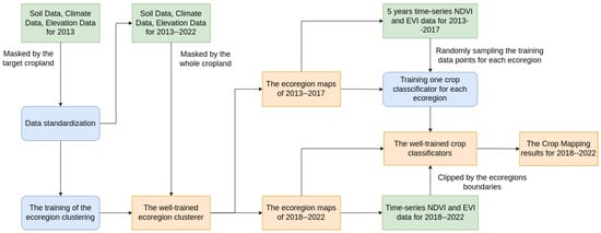
Figure 1.
The system architecture comprises a dynamic ecoregion clustering method and a specific crop classifier for each ecoregion. Inputs to the system are represented by green blocks, system outputs are represented by orange blocks, and system processes are depicted in blue blocks.
3.3. Development of Dynamic Ecoregions
Our study focuses on accurately mapping the growing area of soybean and corn crops before their harvest periods throughout the entire cropland area of the CONUS. To achieve this goal, we utilize a dynamic ecoregion clustering method that relies on soil, climate, elevation, and slope data from various sources. Due to the absence of multi-year soil and topography data, our assumption is that soil quality, elevation, and slope conditions remain relatively stable over time, while climate conditions exhibit variability. Various methods exist for ecoregion clustering, with hierarchical clustering [31] being one such approach known for accommodating datasets with nested or hierarchical structures. However, for our specific scenario, we prefer to adopt a simpler clustering method. This decision is driven by the intention to maintain simplicity in our current approach while preserving compatibility for future integration of multi-year soil and topography data. Consequently, we have chosen a direct clustering method for ecoregion clustering, with the expectation that it will facilitate a smoother transition when more comprehensive data become available in the future.
Each year, we initiate the process by reprojecting the data into a 10,000 m resolution. In the case of soil data, we compute the average metric value by consolidating values from various depths. When dealing with climate data, we determine both the mean and variance for each metric within the specified crop growth period. Notably, when it comes to wind speed, we combine the eastward and northward components to create a total wind speed, discarding the directional information. Then we randomly sample 10,000 points from the target crop region as the training data. Subsequently, we employ the Principal Component Analysis (PCA) method to reduce the data dimensions from 20 (8 for soil conditions, 10 for climate conditions, and 2 for topography conditions) down to 5. We trained our dynamic ecoregion clustering model using the K-means++ method and the pre-processed training data from 2013 and applied it to the entire cropland area, as determined by the cultivated layer of CDL, for the years 2013–2022.
This allows us to identify regions with similar environmental characteristics, which is essential for accurate early crop mapping. In order to determine the optimal number of clusters, we utilize the elbow method to calculate the within-cluster sum of squares (WCSS) value using Equation (1):
where n denotes the total number of ecoregion clusters, denotes the number of pixels contained within cluster i, denotes the vector representing each pixel within cluster i, and represents the centroid vector of cluster i. This allows us to strike a balance between cluster granularity and computational efficiency. If the number of clusters is too small, the environmental similarities may not be unique enough for each cluster, compromising the accuracy of our results. Conversely, if the number of clusters is too large, it may result in excessive computational cost, hindering the practical application of our approach. By finding the optimal number of clusters, we are able to maximize the accuracy of our approach while ensuring its computational feasibility.
The resultant ecoregion maps with different ecoregion numbers, were then used in our crop classification training and testing processes. For instance, Figure 2a displays the entire cropland area of CONUS for the year 2013, as obtained from the CDL layer. We restrict our analysis to the green region that corresponds to the soybean cropland region. We determine the optimal number of ecoregions as 10, identified through the WCSS value. Subsequently, we employ our well-trained ecoregion clustering model to the entire cropland area to generate the ecoregion map for 2013, which is shown in Figure 2c. The ecoregion maps from 2014 to 2022 for soybean mapping are also shown in Figure 3.

Figure 2.
The ecoregion map with 10 clusters of 2013 for soybean mapping. (a) shows the soybean cropland region filtered out by the CDL cultivated layer of 2013, where the green color represents the soybean cropland, and the black color represents the non-soybean cropland. (b) displays the ecoregion map of the soybean cropland region, where each color represents a specific ecoregion. (c) shows the ecoregion map of the entire cropland region, where each color represents a specific ecoregion.
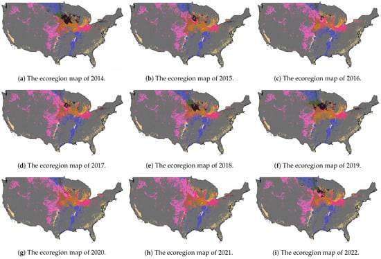
Figure 3.
The dynamic ecoregions maps with 10 clusters for 2014–2022.
To illustrate the variation in time-series vegetation indices of our target crop, we present the time-series average NDVI and EVI curves of soybean for each ecoregion based on ten clusters in 2013 in Figure 4. It is evident that the patterns of these features exhibit significant differences across different ecoregions. To demonstrate distinctions among the distributions of VIs data across various ecoregions, we employ the Maximum Mean Discrepancy (MMD) as a measure. MMD allows us to measure the discrepancy between the distributions of VIs from different ecoregions, providing a quantitative measure of the similarity. Specifically, we compute MMD values between ecoregion 1 and all other ecoregions in our analysis. To ensure statistical robustness, we perform the following steps:
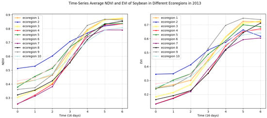
Figure 4.
Time-series average NDVI and EVI of soybean in different ecoregions in 2013. Left for NDVI. Right for EVI.
- We randomly sample 20,000 data points from ecoregion 1.
- For ecoregions 2–10, we also draw random samples of 10,000 data points each.
- For ecoregion 1, we calculate the MMD by comparing two subsets of 10,000 data points each, where the first subset consists of the initial 10,000 data points, and the second subset comprises the last 10,000 data points.
- For the other ecoregions (ecoregions 2–10), we compute the MMD by comparing the initial 10,000 data points from ecoregion 1 with the 10,000 data points from each of the other ecoregions.
The resulting MMD values are summarized in the Table 3. The MMD within ecoregion 1 is notably lower than the MMD between ecoregion 1 and the other ecoregions, providing clear evidence of significant variations in VIs data distribution among different ecoregions.

Table 3.
The MMD values between the ecoregion 1 and each ecoregion.
Moreover, to highlight the varying patterns of VIs within a specific region across disparate ecoregions over different years, we have designated two distinct areas, which changed the ecoregion types between 2014 and 2021, as illustrated in Figure 5. The distribution of soybean VIs data is then presented using t-distributed stochastic neighbor embedding (t-SNE) [32] in Figure 6. Evident disparities in these distributions between the years 2014 and 2021 are discernible, underscoring the fluctuating nature of soybean growth-related VIs data within these designated regions.
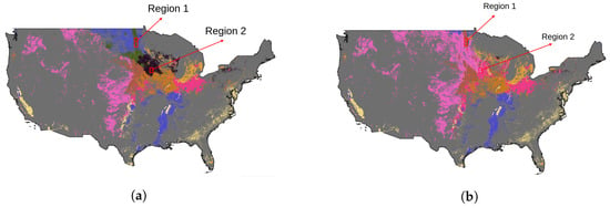
Figure 5.
The sample regions. (a) shows the sample regions with the 2014 ecoregion map. (b) shows the sample regions with the 2021 ecoregion map.
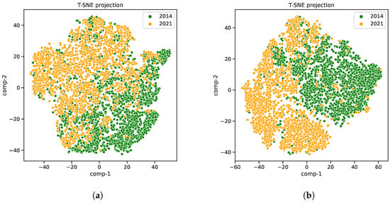
Figure 6.
The soybean VIs data distribution. The x- and y-axes represent the features following dimension reduction using PCA. (a) shows the soybean VIs data distribution in region 1. (b) shows the soybean VIs data distribution in region 2.
3.4. Crop Classification Model
Once the ecoregions are established, a specific early crop mapping classifier can be trained for each different ecoregion based on the cropland region, which is filtered out by the cultivated layer of the CDL. Random Forest classification models have become a popular tool for mapping land cover due to their flexibility in handling nonlinear relationships between input features and class membership, and their intuitive decision rules. During training, the tree grows by recursively partitioning the data into less heterogeneous groups until the desired level of accuracy or purity is achieved. The final model is constructed when all leaf nodes are generated, with each leaf node representing either a pure class or a mixture of two classes, determined by the proportion of training pixels in the node. However, these models are prone to overfitting, which can lead to poor generalization performance. To address this issue, we applied a bagging procedure and trained a random forest consisting of 50 classification tree models. Using a binary target-crop and non-target-crop training dataset, we locate our target crop across the corresponding ecoregion with the well-trained classifier. This approach significantly improved the stability and prediction accuracy of the model.
Since the CDL with the cultivated layer has been available only since 2013, the model was trained and validated in the years 2013–2017 and tested independently in the years 2018–2022.
3.4.1. Model Training within the Training Period
As per the USDA crop calendar, the seeding for corn and soybean typically begins after 1 April. Hence, we extracted time-series MODIS 250 m NDVI and EVI images with a 16-day temporal frequency from April 1st until the middle of July for 2013–2017. For each year, we compose these VIs images into one image as the composed image. Each composed image comprised seven NDVI bands and seven EVI bands. For each training year, we randomly selected 10,000 training sample points from the composed image for each different ecoregion, with half for target-crop points and half for non-target-crop points. Then we merge all the training sample points for the same ecoregion to train the ecoregion-specific crop classification model.
3.4.2. Model Evaluation within the Test Period
In order to evaluate our crop classification model, we first extracted the VIs images and provided the composed images for the years 2018–2022. To assess the effectiveness of our approach, we designed an experiment to compare the results of using a dynamic ecoregions map versus a static one. For the static map, we sample the training points from the 2013–2017 period and classify the target crops for 2018–2022 only using the ecoregion map from 2013, as shown in Figure 2c, with fixed boundaries for each ecoregion. In contrast, for the dynamic map, we sample the training points from the 2013–2017 period based on the ecoregion maps for 2013–2017, as shown in Figure 2c and Figure 3a–d, and classify the target crops for 2018–2022 based on each year’s specific ecoregion map, as shown in Figure 3e–i. The following results show that in most cases the dynamic model outperformed the static model. These findings demonstrate the benefits of using dynamic ecoregion maps in crop classification and highlight the importance of accounting for climate fluctuations when developing land cover maps.
3.4.3. Evaluation Metrics
To evaluate the accuracy of our classification, we used three metrics: Producer’s Accuracy, User’s Accuracy and Overall Accuracy, which are defined in Equations (2)–(4):
where TP, TN, FP, and FN refer to the numerical values in a confusion matrix that correspond to true positive (correctly predicted positive cases), true negative (correctly predicted negative cases), false positive (incorrectly predicted positive cases), and false negative (incorrectly predicted negative cases) outcomes, respectively.
The Producer’s Accuracy represents the map’s accuracy from the map producer’s perspective, indicating the probability that a ground feature is correctly classified by the map. On the other hand, the User’s Accuracy represents the map’s reliability from the user’s perspective, i.e., the probability that a feature on the map is actually present on the ground. The Overall Accuracy typically quantifies the fraction of all CDL pixels, encompassing both target crop and non-target crop pixels, that our crop classification method correctly identifies and maps.
4. Results
4.1. Dynamic Ecoregion Maps
4.1.1. Determine the Elbow Point (Cluster Number)
Rather than directly dividing the CONUS into 500 clusters as in [10], we employed both the elbow method and silhouette method to determine the optimal number of clusters for our approach. This allowed us to balance cluster granularity with computational efficiency, ensuring both accuracy and practicality. Specifically, we calculated the environmental dissimilarities for different cluster numbers in the training year 2013, as shown in Figure 7 and Figure 8. As depicted in Figure 7, we found that ten clusters were optimal, while the dissimilarity significantly decreased with a noticeable reduction starting at ten clusters for both soybean and corn cropland regions. Further insights gleaned from Figure 8 indicate that, for corn, a configuration of two clusters attains the highest silhouette score, while for soybean, this optimal number becomes to five.
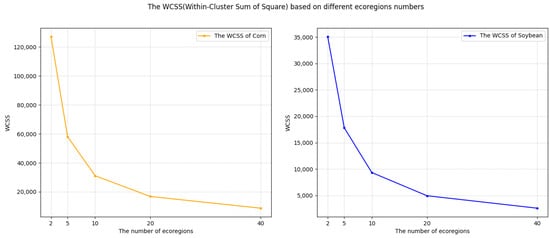
Figure 7.
Within-cluster sum of squares (WCSS) of the environmental dissimilarity based on the pro-processed environmental data for different numbers of ecoregions in the corn cropland region (left) and soybean cropland region (right), during ecoregion clustering training in 2013.
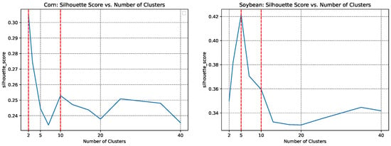
Figure 8.
The silhouette score based on the pro-processed environmental data for different numbers of ecoregions in the corn cropland region (left) and soybean cropland region (right), during ecoregion clustering training in 2013.
As a result, to further evaluate the effectiveness of our approach, we conducted experiments with different cluster numbers, including two, five, and ten, and compare our resulting metrics with those of a static clustering method. By comparing these results, we can confirm the superiority of our dynamic clustering method and demonstrate its capability to identify the target crops accurately. Additionally, we prove that the mapping result with ten ecoregion clusters has the highest accuracy in most cases in the following experiments.
4.1.2. The Visualization of Dynamic Ecoregion Maps
As depicted in Figure 2a, the green area corresponds to the soybean cropland region, whereas the black region represents non-soybean cropland from the year 2013. Notably, we only train the ecoregion clusterer using data from the target cropland region. The resulting ecoregion cluster map for the soybean cropland region is displayed in Figure 2b, while the ecoregion cluster map for the entire cropland region, encompassing both soybean and non-soybean croplands, is illustrated in Figure 2c.
Moreover, in Figure 3, we present the dynamic ecoregion maps for the years 2014–2022 for the soybean mapping task. Notably, the ecoregions in the north and middle of the CONUS exhibit significant changes over the years and especially in 2021, while the ecoregions in the southern region experience relatively less variation over time.
4.2. Comparison of Mapping Result Metrics across the Continental United States
Our experiment serves as a compelling validation of the effectiveness of our approach, as it demonstrates significantly improved accuracy for soybean and corn mapping across the CONUS in most cases when we compare our method with a static one.
4.2.1. Metrics for Soybean Mapping
In Table 4, we present a detailed comparison of the Producer’s Accuracy and the User’s Accuracy between our dynamic ecoregion method and the static ecoregion method. Notably, we observe consistent trends in the User’s Accuracy across different years. With the utilization of ten different ecoregions, our dynamic ecoregion method achieves the highest Producer’s Accuracy for soybean mapping in all years except for 2018. In that specific year, our method employing five different ecoregions yields the highest Producer’s Accuracy. Furthermore, our analysis reveals that the most significant improvements in Producer’s Accuracy using our dynamic ecoregion method occurred in 2018 and 2021. Specifically, in 2018, we observed an increase in Producer’s Accuracy from 59.04 to 62.74%, representing a substantial improvement of 3.7%. Similarly, in 2021, our dynamic ecoregion method yielded an impressive improvement of 3.46%, increasing User’s Accuracy from 69.87 to 73.33%. These findings emphasize the efficacy of our approach in accurately identifying and early mapping soybean crops across diverse environmental conditions.

Table 4.
The experiment metrics for soybean early crop mapping based on different numbers of ecoregions. Bold numbers indicate the best results for each experimental group.
Regarding the User’s Accuracy, our dynamic ecoregion method with two, five and ten different ecoregions outperforms the static ecoregion method in most years. However, in 2020, the static ecoregion map exhibited better performance in terms of User’s Accuracy. This exceptional result suggests that the static ecoregion map might offer advantages under specific circumstances, but overall, our dynamic ecoregion method consistently demonstrates superior accuracy. The mapping result with ten ecoregion clusters has the highest accuracy in most cases in the following experiments.
Additionally, we conducted an experiment to compare early crop mapping results using both NDVI and EVI against using only NDVI. Table 5 displays the Producer’s Accuracy and User’s Accuracy for the method exclusively utilizing NDVI. Notably, except for the year 2020, the Producer’s Accuracy when employing NDVI and EVI is consistently higher than when using only NDVI. In most instances, the NDVI and EVI combination yields an approximately 2% improvement. Furthermore, when considering User’s Accuracy across all years, the NDVI and EVI approach consistently outperforms the exclusive use of NDVI. Particularly, in 2021, the NDVI and EVI method achieves a remarkable 5.81% increase in accuracy compared to the NDVI-only approach. Consequently, in this study, we adopt the combined use of NDVI and EVI for our early crop-mapping models.

Table 5.
The experiment metrics for corn early crop mapping only using NDVI. Dynamic and static method with 10 ecoregions. Normal presents the early crop mapping method without ecoregions. Bold numbers indicate the best results for each experimental group.
Figure 9 presents our soybean early mapping result for the CONUS in 2021. To demonstrate the accuracy of our approach, we selected a sample test region and compared our soybean mapping result with 250 m resolution to the soybean ground truth with 30 m resolution from the CDL layer. Our result exhibits a broad-level spatial agreement with the CDL, indicating the effectiveness of our approach. However, due to the coarser resolution of MODIS products, our mapping result lacks sharpness and accuracy along the field boundaries. Furthermore, Figure 10a illustrates the pixel-wise overall accuracy using the dynamic method, where the color scale indicates the accuracy, with greener colors representing higher overall accuracy. Figure 10b highlights the regions where the pixel-wise overall accuracy from the dynamic method outperforms the static method. It is evident that the dynamic method exhibits notably higher overall accuracy than the static method, particularly within regions where there has been a shift in ecoregion types between 2013 and 2021. This contrast is particularly pronounced in the northern part of the CONUS.
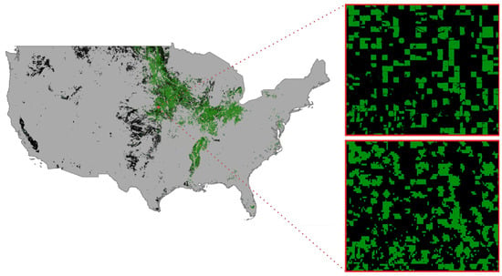
Figure 9.
The soybean cropping result for the entire conterminous U.S. land area in 2021 (left). The ground truth of soybean cropland in a sample test region at 30 m resolution from the CDL layer (Right Top), and our soybean mapping result in the sample test region at 250 m resolution (Right Bottom).
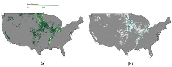
Figure 10.
Soybean mapping pixel-wise overall accuracy for 2021. (a) illustrates the pixel-wise overall accuracy using the dynamic method, where the color scale indicates the accuracy, with greener colors representing higher overall accuracy. (b) highlights the regions where the pixel-wise overall accuracy from the dynamic method outperforms the static method.
4.2.2. Metrics for Corn Mapping
Given the successful performance of our soybean mapping approach using ten different ecoregions and computational efficiency considerations, we extend our experiment to map corn crops using the same approach. As shown in Table 6, our dynamic ecoregion-mapping method demonstrates similar levels of Producer’s Accuracy across different years, except for 2021, where we observe a notable improvement from 82.04 to 83.83%, representing a 1.79% increase over the static method. In terms of User’s Accuracy, our dynamic approach outperforms the static method, with the greatest improvement observed in 2019 from 76.62 to 77.72%. Overall, these results demonstrate the effectiveness of our dynamic ecoregion-mapping approach for mapping corn crops, with improvements in both Producer’s Accuracy and User’s Accuracy compared to the static method. Similar to the soybean mapping result, Figure 11 presents our corn-mapping results for the CONUS in 2021.

Table 6.
The experiment metrics for corn early crop mapping based on ten ecoregions. Bold numbers indicate the best results for each experimental group.
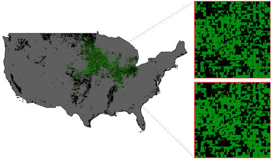
Figure 11.
The corn cropping result for the entire conterminous U.S. land area in 2021 (left). The ground truth of soybean cropland in a sample test region at 30 m resolution from the CDL layer (Right Top), and our corn mapping result in the sample test region at 250 m resolution (Right Bottom).
To confirm our dynamic approach’s superiority over the static method, we conducted another experiment focusing solely on the ecoregion-changing regions in the corn-growing area. As shown in Table 7, our dynamic method’s User’s Accuracy outperformed the static method in almost all cases, except for 2021. For Producer’s Accuracy, both methods showed improvement or decline in different years. Therefore, we calculated the overall accuracy, which showed that the dynamic method in most cases outperformed the static method, with the largest improvement observed in 2020 from 71.76 to 74.98%. These results confirm the effectiveness of our dynamic ecoregion mapping approach for corn crops, especially in regions undergoing rapid ecoregion changes.

Table 7.
The metrics of corn mapping based on ecoregion-changed fields. Bold numbers indicate the best results for each experimental group.
5. Discussion
Our study demonstrates that our approach, incorporating dynamic ecoregion clustering and random forest classification, yields markedly higher accuracy compared to the static clustering method in the context of early crop mapping for target crops such as soybean and corn across the entire cropland region.
We employed the elbow method and silhouette method to ascertain the optimal number of ecoregion clusters. This approach allowed us to strike a balance between accuracy and computational efficiency, enabling us to achieve satisfactory early crop mapping results while conserving computational resources. However, there exists a limitation: when there is significant climate variability affecting the vegetation index (VIs) patterns of the target crops, but not substantial enough to alter the ecoregion boundaries, our system may struggle to address this scenario effectively. As illustrated in Figure 10a, the overall accuracy is notably low in the Southern USA. This issue becomes apparent when examining Figure 2c and Figure 3, where, for the Southern USA region (depicted in blue), the ecoregion remains unchanged from 2013 to 2022. Consequently, our method fails to account for VIs pattern fluctuations in this region during this time period.
In our investigations, we observe that our dynamic ecoregion method, employing two, five, and ten distinct ecoregions, typically outperforms the static ecoregion method across most years in early soybean mapping. Particularly, the ecoregion configuration with ten divisions yields the most accurate outcomes. However, an interesting anomaly arises in the year 2020, where the static ecoregion map exhibits superior User’s Accuracy performance. This divergence implies that the static ecoregion map could possess advantages in specific scenarios, although overall, our dynamic ecoregion method generally exhibits enhanced accuracy. Notably, a comparison of pixel-wise overall accuracy between the dynamic and static methods for the soybean mapping underscores that the dynamic approach significantly outperforms the static approach in regions where shifts in ecoregion types between 2013 and 2021 have occurred. This contrast is particularly evident in the northern CONUS, confirming the enhanced robustness of our method against climate fluctuations between different years.
Interestingly, we find that the dynamic method outperforms the static method significantly in soybean mapping, while the improvement is less pronounced in corn mapping. Although the exact cause has not been explored in this paper, it is plausible that climate fluctuations exert a more substantial impact on soybean growing than on corn growing.
In conclusion, our proposed approach not only attests to its efficacy in terms of soybean and corn mapping, but also highlights the benefits of dynamic ecoregion clustering in coping with the intricate influences of climate fluctuations on crop mapping accuracy. Furthermore, our result map provides early insights into crop conditions, significantly preceding the CDL release. This timeliness is pivotal for making informed decisions early in the growing season. While the USDA unveils its CDL layer in January or February of the following year, our results are accessible by mid-July of the same year, offering information approximately 7 months ahead of the CDL. In addition, producing and updating a 250 m map proves to be more resource-efficient when compared to the maintenance of a nationwide 30 m map, particularly for research and monitoring purposes. However, the lower resolution of MODIS VIs data causes reduced accuracy in mapping target crops, when contrasted with Sentinel-2 and Landsat data. This decrease in resolution results in the loss of finer details and subtleties within the agricultural landscape, thereby presenting challenges in distinguishing between various crop types and detecting smaller-scale changes. It is important to note that this limitation constitutes a constraint within our work.
6. Conclusions
This paper introduces an innovative approach for early crop mapping across the entire land area of the CONUS by utilizing NDVI and EVI data combined with a dynamic ecoregion clustering technique. Unlike static ecoregion clustering, which generates a single unchanging ecoregion map, our dynamic approach results in a unique ecoregion map for each year. This dynamic strategy enables us to incorporate the year-to-year climate variations that significantly influence crop growth, thereby heightening the precision of our crop mapping process.
With the ecoregion maps for 2013–2022 established by the dynamic ecoregion clustering, a specific early crop mapping classifier can be trained for each different ecoregion. We used a bagging procedure and trained a random forest consisting of 50 classification tree models to locate our target crop for each ecoregion separately across the entire cropland region of the CONUS. The model was trained and validated in the years 2013–2017 and tested independently in the years 2018–2022. The results showed that the dynamic clustering method achieved significantly higher accuracy than the static clustering method. Our method has significant implications for forecasting crop yield and food production for countries.
In our future research endeavors, we intend to broaden the scope of our work by applying the dynamic ecoregion method to estimate target crop yields. This represents a crucial evolution of our current approach, as it will enable us to not only identify and map crops within distinct ecological regions, but also predict and quantify their potential yields. By harnessing the power of this method, we aim to provide valuable insights into agricultural productivity, aiding farmers, policymakers, and researchers in making informed decisions.
Author Contributions
Conceptualization, Y.W.; methodology, Y.W.; software, Y.W.; validation, Y.W.; formal analysis, Y.W.; investigation, Y.W.; resources, Y.W.; data curation, Y.W.; writing—original draft preparation, Y.W.; writing—review and editing, H.H.; visualization, Y.W.; supervision, R.S.; project administration, H.H.; funding acquisition, R.S. All authors have read and agreed to the published version of the manuscript.
Funding
This research received no external funding.
Data Availability Statement
Not applicable.
Conflicts of Interest
The authors declare no conflict of interest.
References
- Van Klompenburg, T.; Kassahun, A.; Catal, C. Crop yield prediction using machine learning: A systematic literature review. Comput. Electron. Agric. 2020, 177, 105709. [Google Scholar] [CrossRef]
- Clevers, J.; Büker, C.; Van Leeuwen, H.; Bouman, B. A framework for monitoring crop growth by combining directional and spectral remote sensing information. Remote Sens. Environ. 1994, 50, 161–170. [Google Scholar] [CrossRef]
- Karthikeyan, L.; Chawla, I.; Mishra, A.K. A review of remote sensing applications in agriculture for food security: Crop growth and yield, irrigation, and crop losses. J. Hydrol. 2020, 586, 124905. [Google Scholar] [CrossRef]
- Ramirez Cabral, N.Y.; Kumar, L.; Shabani, F. Global alterations in areas of suitability for maize production from climate change and using a mechanistic species distribution model (CLIMEX). Sci. Rep. 2017, 7, 1–13. [Google Scholar] [CrossRef] [PubMed]
- Sonobe, R.; Yamaya, Y.; Tani, H.; Wang, X.; Kobayashi, N.; Mochizuki, K.i. Mapping crop cover using multi-temporal Landsat 8 OLI imagery. Int. J. Remote Sens. 2017, 38, 4348–4361. [Google Scholar] [CrossRef]
- Gao, F.; Anderson, M.C.; Zhang, X.; Yang, Z.; Alfieri, J.G.; Kustas, W.P.; Mueller, R.; Johnson, D.M.; Prueger, J.H. Toward mapping crop progress at field scales through fusion of Landsat and MODIS imagery. Remote Sens. Environ. 2017, 188, 9–25. [Google Scholar] [CrossRef]
- Skakun, S.; Vermote, E.; Roger, J.C.; Franch, B. Combined use of Landsat-8 and Sentinel-2A images for winter crop mapping and winter wheat yield assessment at regional scale. AIMS Geosci. 2017, 3, 163. [Google Scholar] [CrossRef]
- Belgiu, M.; Csillik, O. Sentinel-2 cropland mapping using pixel-based and object-based time-weighted dynamic time warping analysis. Remote Sens. Environ. 2018, 204, 509–523. [Google Scholar] [CrossRef]
- Wardlow, B.D.; Egbert, S.L. Large-area crop mapping using time-series MODIS 250 m NDVI data: An assessment for the U.S. Central Great Plains. Remote Sens. Environ. 2008, 112, 1096–1116. [Google Scholar] [CrossRef]
- Konduri, V.S.; Kumar, J.; Hargrove, W.W.; Hoffman, F.M.; Ganguly, A.R. Mapping crops within the growing season across the United States. Remote Sens. Environ. 2020, 251, 112048. [Google Scholar] [CrossRef]
- HAO, P.; Tang, H.; CHEN, Z.; Le, Y.; Wu, M. High resolution crop intensity mapping using harmonized Landsat-8 and Sentinel-2 data. J. Integr. Agric. 2019, 18, 2883–2897. [Google Scholar] [CrossRef]
- Song, X.; Potapov, P.V.; Krylov, A.; King, L.; Di Bella, C.M.; Hudson, A.; Khan, A.; Adusei, B.; Stehman, S.V.; Hansen, M.C. National-scale soybean mapping and area estimation in the United States using medium resolution satellite imagery and field survey. Remote Sens. Environ. 2017, 190, 383–395. [Google Scholar] [CrossRef]
- Wardlow, B.D.; Egbert, S.L. A comparison of MODIS 250-m EVI and NDVI data for crop mapping: A case study for southwest Kansas. Int. J. Remote Sens. 2010, 31, 805–830. [Google Scholar] [CrossRef]
- Leng, G.; Huang, M. Crop yield response to climate change varies with crop spatial distribution pattern. Sci. Rep. 2017, 7, 1463. [Google Scholar] [CrossRef]
- Choudhary, K.; Shi, W.; Dong, Y.; Paringer, R. Random Forest for rice yield mapping and prediction using Sentinel-2 data with Google Earth Engine. Adv. Space Res. 2022, 70, 2443–2457. [Google Scholar] [CrossRef]
- Zhong, L.; Gong, P.; Biging, G.S. Efficient corn and soybean mapping with temporal extendability: A multi-year experiment using Landsat imagery. Remote Sens. Environ. 2014, 140, 1–13. [Google Scholar] [CrossRef]
- Skakun, S.; Franch, B.; Vermote, E.; Roger, J.C.; Becker-Reshef, I.; Justice, C.; Kussul, N. Early season large-area winter crop mapping using MODIS NDVI data, growing degree days information and a Gaussian mixture model. Remote Sens. Environ. 2017, 195, 244–258. [Google Scholar] [CrossRef]
- Massey, R.; Sankey, T.T.; Congalton, R.G.; Yadav, K.; Thenkabail, P.S.; Ozdogan, M.; Meador, A.J.S. MODIS phenology-derived, multi-year distribution of conterminous US crop types. Remote Sens. Environ. 2017, 198, 490–503. [Google Scholar] [CrossRef]
- Hargrove, W.W.; Hoffman, F.M. Potential of multivariate quantitative methods for delineation and visualization of ecoregions. Environ. Manag. 2004, 34, S39–S60. [Google Scholar] [CrossRef] [PubMed]
- Hoffman, F.M.; Hargrove, W.W.; Mills, R.T.; Mahajan, S.; Erickson, D.J.; Oglesby, R.J. Multivariate Spatio-Temporal Clustering (MSTC) as a data mining tool for environmental applications. In Proceedings of the 4th International Congress on Environmental Modelling and Software, Barcelona, Catalonia, Spain, 1 July 2008. [Google Scholar]
- Alami Machichi, M.; El Mansouri, L.; Imani, Y.; Bourja, O.; Hadria, R.; Lahlou, O.; Benmansour, S.; Zennayi, Y.; Bourzeix, F. CerealNet: A Hybrid Deep Learning Architecture for Cereal Crop Mapping Using Sentinel-2 Time-Series. Informatics 2022, 9, 96. [Google Scholar] [CrossRef]
- Zhong, L.; Yu, L.; Li, X.; Hu, L.; Gong, P. Rapid corn and soybean mapping in US Corn Belt and neighboring areas. Sci. Rep. 2016, 6, 1–14. [Google Scholar] [CrossRef] [PubMed]
- Cai, Y.; Guan, K.; Peng, J.; Wang, S.; Seifert, C.; Wardlow, B.; Li, Z. A high-performance and in-season classification system of field-level crop types using time-series Landsat data and a machine learning approach. Remote Sens. Environ. 2018, 210, 35–47. [Google Scholar] [CrossRef]
- USDA. District and County Boundary Maps by State. 2023. Available online: https://www.nass.usda.gov/Charts_and_Maps/Crops_County/boundary_maps/indexgif.php (accessed on 29 March 2023).
- Boryan, C.; Yang, Z.; Mueller, R.; Craig, M. Monitoring US agriculture: The US department of agriculture, national agricultural statistics service, cropland data layer program. Geocarto Int. 2011, 26, 341–358. [Google Scholar] [CrossRef]
- Poggio, L.; De Sousa, L.M.; Batjes, N.H.; Heuvelink, G.; Kempen, B.; Ribeiro, E.; Rossiter, D. SoilGrids 2.0: Producing soil information for the globe with quantified spatial uncertainty. Soil 2021, 7, 217–240. [Google Scholar] [CrossRef]
- Hersbach, H.; Bell, B.; Berrisford, P.; Hirahara, S.; Horányi, A.; Muñoz-Sabater, J.; Nicolas, J.; Peubey, C.; Radu, R.; Schepers, D.; et al. The ERA5 global reanalysis. Q. J. R. Meteorol. Soc. 2020, 146, 1999–2049. [Google Scholar] [CrossRef]
- Danielson, J.J.; Gesch, D.B. Global Multi-Resolution Terrain Elevation Data 2010 (GMTED2010). 2011. Available online: https://www.usgs.gov/centers/eros/science/usgs-eros-archive-digital-elevation-global-multi-resolution-terrain-elevation (accessed on 13 July 2018).
- Gorelick, N.; Hancher, M.; Dixon, M.; Ilyushchenko, S.; Thau, D.; Moore, R. Google Earth Engine: Planetary-scale geospatial analysis for everyone. Remote Sens. Environ. 2017, 202, 18–27. [Google Scholar] [CrossRef]
- Bahmani, B.; Moseley, B.; Vattani, A.; Kumar, R.; Vassilvitskii, S. Scalable k-means++. arXiv 2012, arXiv:1203.6402. [Google Scholar] [CrossRef]
- Murtagh, F.; Contreras, P. Algorithms for hierarchical clustering: An overview. Wiley Interdiscip. Rev. Data Min. Knowl. Discov. 2012, 2, 86–97. [Google Scholar] [CrossRef]
- Van der Maaten, L.; Hinton, G. Visualizing data using t-SNE. J. Mach. Learn. Res. 2008, 9, 2579–2605. [Google Scholar]
Disclaimer/Publisher’s Note: The statements, opinions and data contained in all publications are solely those of the individual author(s) and contributor(s) and not of MDPI and/or the editor(s). MDPI and/or the editor(s) disclaim responsibility for any injury to people or property resulting from any ideas, methods, instructions or products referred to in the content. |
© 2023 by the authors. Licensee MDPI, Basel, Switzerland. This article is an open access article distributed under the terms and conditions of the Creative Commons Attribution (CC BY) license (https://creativecommons.org/licenses/by/4.0/).