A New Remote Hyperspectral Imaging System Embedded on an Unmanned Aquatic Drone for the Detection and Identification of Floating Plastic Litter Using Machine Learning

Abstract

This paper presents a new Remote Hyperspectral Imaging System (RHIS) embedded on an Unmanned Aquatic Drone (UAD) for plastic detection and identification in coastal and freshwater environments. This original system, namely the Remotely Operated Vehicle of the University of Littoral Côte d’Opale (ROV-ULCO), works in a near-field of view, where the distance between the hyperspectral camera and the water surface is about 45 cm. In this paper, the new ROV-ULCO system with all its components is firstly presented. Then, a hyperspectral image database of plastic litter acquired with this system is described. This database contains hyperspectral data cubes of different plastic types and polymers corresponding to the most-common plastic litter items found in aquatic environments. An in situ spectral analysis was conducted from this benchmark database to characterize the hyperspectral reflectance of these items in order to identify the absorption feature wavelengths for each type of plastic. Finally, the ability of our original system RHIS to automatically recognize different types of plastic litter was assessed by applying different supervised machine learning methods on a set of representative image patches of marine litter. The obtained results highlighted the plastic litter classification capability with an overall accuracy close to 90%. This paper showed that the newly presented RHIS coupled with the UAD is a promising approach to identify plastic waste in aquatic environments.

1. Introduction

The high and rapidly increasing levels of plastic litter in aquatic environments represent a serious environmental problem at a global scale, negatively affecting aquatic life and biodiversity, ecosystems, livelihoods, fisheries, maritime transport, recreation, tourism, and economies. To address this problem, the research community is always looking for novel devices, tools, and methods to detect, identify, and quantify plastic litter more rapidly and efficiently [1,2,3,4]. Monitoring methods such as visual counting or sampling using nets are labor-intensive, whereas current remote observation (from spaceborne or airborne platforms) has some limitations in detecting and identifying plastic litter. Therefore, it is necessary to develop an innovative remote sensing system able to automatically detect and identify plastic litter in order to study pollution sources properly, to improve the survey assessments, and to support the implementation of mitigation measures [1,2,3,4,5].

Recently, remote sensing systems, which acquire hyperspectral images, were used to detect, identify, and characterize marine plastics [5,6]. In general, hyperspectral imaging systems can collect the information of hundreds of wavelengths ranging from Visible (VIS: 400–750 nanometers) to Near-Infra-Red (NIR: 750–1100 nanometers) and Short-Wave Infra-Red (SWIR: 1100–2500 nanometers) [7,8,9]. Despite being an expensive and complex technology, it is robust in detecting and identifying plastic litter. Tasseron et al. identified six types of plastic that are the most-abundant in freshwater systems and rivers [3]. These types are Low-Density PolyEthylene (LDPE), High-Density PolyEthylene (HDPE), PolyStyrene (PS), PolyVinyl Chloride (PVC), PolyPropylene (PP), and PolyEthylene Terephthalate (PET). The authors used two Specim hyperspectral cameras: FX10 (VIS-NIR) and FX17 (NIR-SWIR), to detect and identify these types of plastics in the laboratory, then they compared this identification using Sentinel-2 and Worldview-3 satellite images. Zhou et al. used public spectral libraries extracted from the airborne hyperspectral images of the HyMap whisk-broom sensor and two push-broom scanners, the HySpex Mjolnir S-620 (NEO) and HySpex-SWIR-320, to create a hyperspectral database with mixed pixels of different plastic and non-plastic materials [5]. The identified plastic types were PolyEthylene (PE), PP, PVC, PET, PS, and industrial plastic types such as: Acrylonitrile Butadiene Styrene (ABS), Ethylene Vinyl Acetate (EVA), PolyAmide (PA), PolyCarbonate (PC), and PolyMethyl MethAcrylate (PMMA). Then, they compared this identification using GF-5 and PRISMA satellite images. Moshtaghi et al. conducted an analysis of a controlled environment on different plastic types: PET, PP, PolyESTer (PEST), and LDPE, to better understand the effect of water absorption on their spectral reflectance [6]. They showed the importance of using spectral wavebands in both visible and the short-wave-infrared spectrum for litter detection, especially when plastics are wet, which is often the case in natural aquatic environments. Balsi et al. separated two plastic types of PE (LDPE and HDPE) and PET objects using a hyperspectral camera in the NIR–SWIR range (900–1700 nm) embedded on an Unmanned Aerial Vehicle (UAV) [10]. This brief state-of-the-art of plastic litter identification with hyperspectral cameras reveals the plastic types that are the most-abundant in seawater, freshwater, and rivers, even though the distribution, types, and amount of plastic waste are variable [3,11]. Moreover, most of these studies showed that the use of NIR and SWIR hyperspectral imaging systems between 900 nm and 1700 nm are promising to recognize plastics because the different types of plastics have distinct hyperspectral reflectance in this spectrum range [6,7]. Using a limited spectral range can also help reduce the cost of the hyperspectral imaging system and the huge amount of hyperspectral information to be processed. For this reason, our research work focused on the use of such a hyperspectral imaging system for remote plastic litter detection.

Currently, most of the Earth Observation (EO) detection methods for floating plastic waste are based on satellite images [3,9,12,13,14,15], airborne platforms [16,17,18,19,20], UAVs and drones [10,15,16,20,21]. Figure 1 gives the remote conceptual framework for marine litter detection proposed by Freitas et al. [22]. It illustrates the use of different devices that embed remote sensors for the observation of plastic litter at different distances and scales from the ground. Satellites are able to provide much information with a good revisiting time over extended areas, which could make them a suitable tool for plastic litter detection. However, current satellite on-board sensors such as multispectral imaging sensors are not designed for plastic litter detection. On the one hand, their spatial resolution is not accurate enough to detect and identify marine litter individually. On the other hand, their spectral information is far from ideal for solving the problem due to the reduced number of available wavelengths [3,5,23]. For example, the European Sentinel satellite “Sentinel-2” has three different spatial resolutions (10, 20, or 60 m/pixel) at different wavelengths varying from the VIS to the SWIR [3,9,16]. Airborne platforms, UAVs, and drones equipped with hyperspectral imaging systems can analyze some requirements at the spatial and spectral data level, but they also have some limitations in spatial and/or spectral resolution [8,10,16]. Moreover, satellites and aerial images need to apply atmospheric correction methods on the data to extract the hyperspectral reflectance.

One way to overcome such limitations is to develop a hyperspectral system that works in the near-field and acquires hyperspectral images with a high spatial resolution and a high number of spectral bands. In this context, our contribution, proposed in this paper, was the development of a new Remote Hyperspectral Imaging System (RHIS) embedded on an Unmanned Aquatic Drone (UAD), namely the Remotely Operated Vehicle of the University of Littoral Côte d’Opale (ROV-ULCO), as shown in Figure 1. To our knowledge, such a system is a real technological innovation that has never been presented in the literature and, therefore, constitutes the novelty of our work. Our main objectives were (1) to develop new technologies for the perception and detection of plastic waste, (2) to reduce time consumption during a study, and (3) to generalize an accurate tool to quantify, qualify, and identify polymers of floating plastic litter. This study, thus, contributes to the ongoing research efforts to develop new tools and methodologies for plastic litter detection.

Although the use of hyperspectral imaging provides a large amount of information, the problem of marine litter detection and identification is still complex due to the number of different types of marine waste, especially for plastic materials present in aquatic environments, and the difficulty to recognize their nature by image analysis because of their high shape, size, opacity, and polymer variabilities [10,11,24]. Indeed, floating plastic litter can be perceived differently depending on its position, its orientation, or its speed in front of the camera and the lighting device, which can generate shadows and specular reflection, depending on the opacity of its material or depending on whether its surface is either wet or dry and mixed with other materials. In order to reproduce these different scenarios, it is important to first carry out experiments under laboratory-controlled conditions. Furthermore, dealing with hyperspectral data is computationally expensive, and it is quite challenging to collect and manually label data for all types of existing plastic marine litter [3,5,10,11].

In this study, our general focus aimed to assess the capability of the proposed ROV-ULCO system to automatically recognize different types of plastic waste in aquatic environments with classical machine learning methods. For this purpose, waste samples representative of the most-common marine litter items found in the coastal environment were collected. This collection contained different plastic types (HDPE, LDPE, PET, PP, PVC, PS, etc.) and other materials such as wood, paper, rubber, and vegetation. Hyperspectral images of these waste items were then acquired by the RHIS system in laboratory-controlled conditions to build a benchmark database. RHIS provides high-spatial-resolution images and hyperspectral data cubes that cover the NIR (900 nm) to SWIR (1700 nm) range of the electromagnetic spectrum. From this database, an in situ spectral analysis was carried out to check the compliance of the spectra with the literature. Standard machine learning methods were then applied to evaluate the plastic waste recognition performance of our system.

The second section of the paper first presents the ROV-ULCO system with all its components, as well as the collected waste samples used in the experiments. This section describes how the waste samples are scanned by the ROV-ULCO to provide hyperspectral images of the proposed benchmark database. Two kinds of datasets were then derived from this database. The first dataset was constituted by the mean spectral reflectance computed over various parts of each marine litter sample observed under different conditions. This dataset was used to conduct an in situ spectral analysis in order to characterize each type of marine litter by a reference hyperspectral reflectance, as described in Section 3. This analysis aimed to compare the absorption features of each reference hyperspectral reflectance with the literature and thus confirmed which wavelengths were the most-efficient to discriminate the different plastic types. The second dataset was a set of same-sized image patches manually selected from the whole hyperspectral images and labeled with the ground-truth of each available marine litter category. Section 4 presents the experiments conducted with this dataset in order to assess the ability of our original RHIS to recognize different categories of marine litter. In this section, several supervised machine learning models, such as K-Nearest Neighbors (KNNs), Support Vector Machines (SVMs), and Artificial Neural Networks (ANNs), were trained on a set of training image patches. Then, the best-trained models were used to evaluate their performance on the testing image patches of the marine litter so that the testing patches were independent of the training ones to reproduce realistic conditions. Finally, the conclusion highlights that the ROV-ULCO is a promising approach to detect and identify plastic litter in aquatic environments.

2. Materials

This section describes the materials used in this study. The new remote hyperspectral imaging ROV-ULCO system is first presented with all its components in Section 2.1. The experimental setup to conduct the acquisitions with this system is then described in Section 2.2. This setup aimed to create a benchmark hyperspectral image database of plastic litter in a controlled laboratory environment, which reproduces different real situations. This database is presented in Section 2.3.

2.1. The ROV-ULCO System

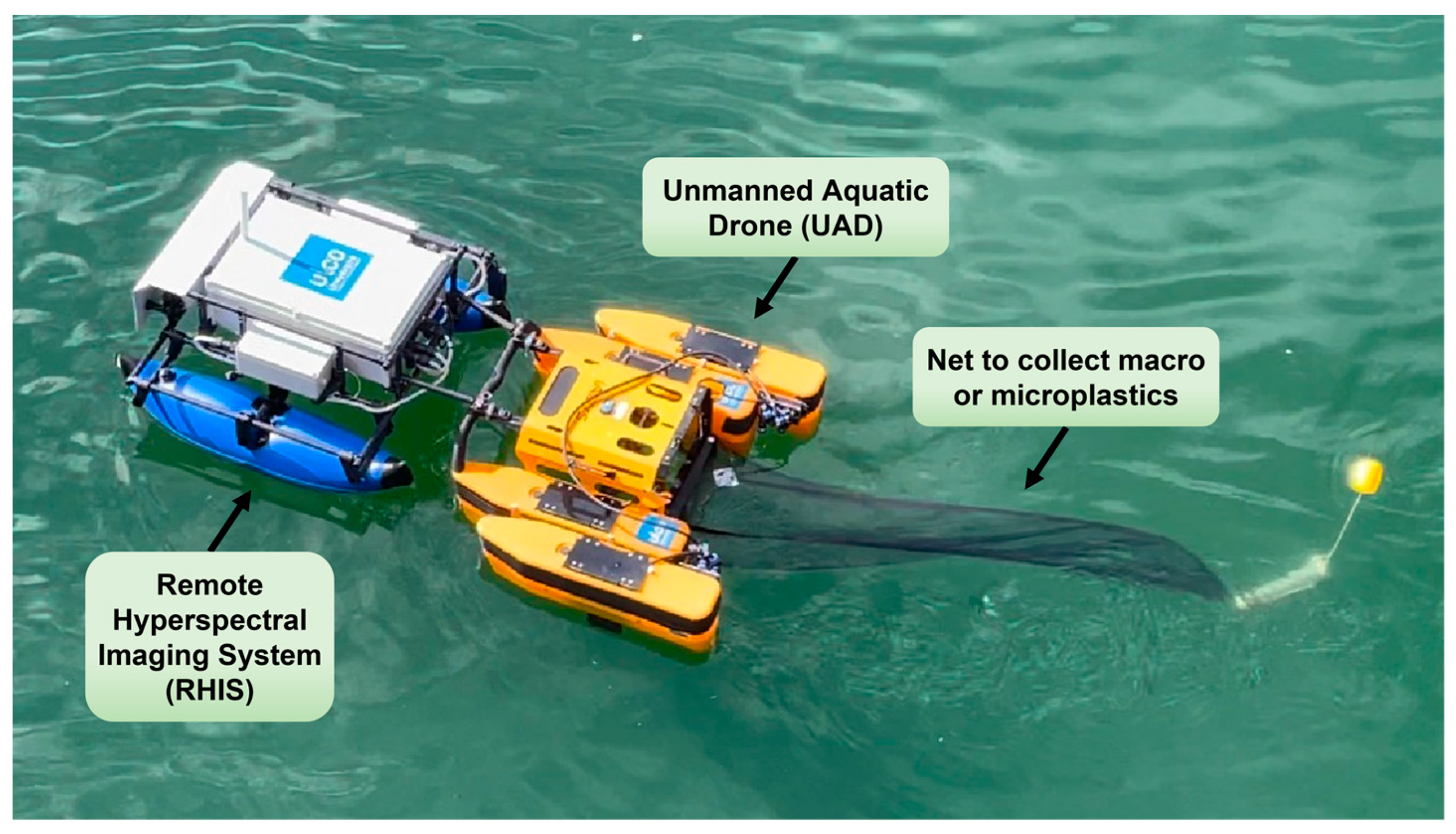
The ROV-ULCO system, illustrated in Figure 2, is constituted of two subsystems: a new Remote Hyperspectral Imaging System (RHIS) and an Unmanned Aquatic Drone (UAD).

The UAD is an aquatic surface drone, named Jellyfishbot, specifically designed for removing floating debris [25]. It is equipped with two propulsions, which are located under the two floating parts, and a remote control and communication system. The aquatic drone can reach a top speed of 2 knots and can have autonomy in terms of power that is greater than 2 h. The UAD was tailored at the University of Littoral (ULCO) to enable plastic material sampling in different water bodies, even in confined and hard-to-reach areas such as small waterways, estuaries, or rivers [25].

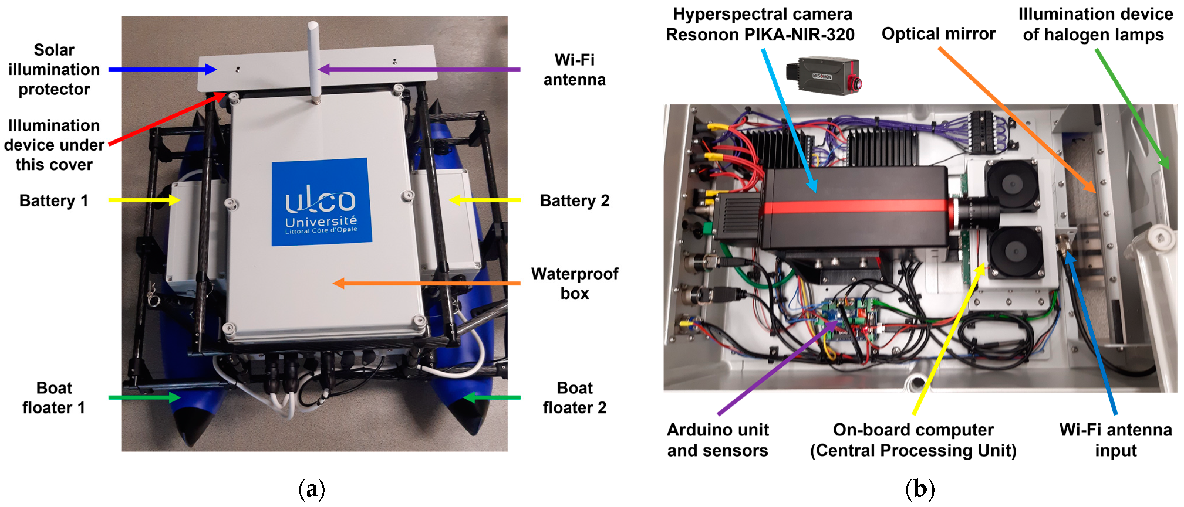
The RHIS is connected at the front of the UAD in order to push it at the water surface. This original imaging system was structured around the following main outside elements (Figure 3):

• Two inflatable boat floaters;
• Two batteries (each inside a removable waterproof case);
• An illumination device of halogen lamps;
• Protections against solar illumination;
• A long-range WiFi antenna to communicate remotely;
• A waterproof box that contains the following inside components (Figure 3b):

  ○

  A line-scan hyperspectral camera (Resonon PIKA-NIR-320) with a 12 mm focal length objective lens;

  ○

  An optical mirror system;

  ○

  An Arduino unit that controls two temperature sensors and a water velocity sensor via an integrated board.

  ○

  An industrial Central Processing Unit (CPU) as the on-board computer;

The system enclosures are certified waterproof up to a 1.5 m depth at atmospheric pressure and for 30 min with an Ingress Protection (IP) rating of IP67.

The usage of the ROV-ULCO is limited to the observation of marine litter floating on the surface of the water. The current prototype is not designed to detect occluded objects that are not visible at the first observation layer or that are completely submerged under the water, which absorbs SWIR light depending on the depth.

The ROV-ULCO can travel more than 2 km with 1 h of autonomy at a maximum speed of 2 knots, before returning to replace the interchangeable batteries and continue the observation.

Hyperspectral images are stored only when marine litter is present under the RHIS. The recorded images are then processed offline to recognize the type of waste observed by the camera.

The Resonon PIKA-NIR-320 is a line-scan (also called push-broom) hyperspectral camera that covers the NIR to SWIR spectral range (900–1700 nm) with 164 spectral bands. The total number of spectral channels delivered by this camera is actually 168, with bands extending beyond both edges of the spectral range. Its resolution is 320 spatial pixels per line with a pixel size of 30 µm, and its line rate reaches up to 520 Hz. The main characteristics of the PIKA-NIR-320 hyperspectral camera are described in the Supplementary Materials (Datasheet S1) (now referred to as Pika IR hyperspectral camera: https://resonon.com/Pika-IR, accessed on 28 March 2023). This line-scan imager collects data one line at a time, and a two-dimensional image is completed by assembling line-by-line the multiple line-images acquired successively as the object is translated. To obtain hyperspectral data, signals from each pixel of a line-image enter at the same time into a spectrometer, which provides the spectrum of incoming light intensity as a function of wavelength for every pixel of the image. The two-dimensional image thus-acquired can be interpreted as a stack of single-band grayscale images, called a data cube, where each image of the stack corresponds to a different wavelength. This hyperspectral camera is provided with the SpectrononPro software, version 3.4.4 (Spectronon software, Hyperspectral Software: https://resonon.com/software, accessed on 28 March 2023) to acquire data.

In order to ensure the stability of the system, the RHIS was designed in such a way that the center of gravity of the camera is as close as possible to the surface of the water. This is the reason why the camera is positioned horizontally with its optical axis parallel to the water surface. The ROV-ULCO is remotely controlled so that marine litter floating on the water is scanned by the RHIS. The latter operates in a very near-field to detect floating marine litter, where the distance between the hyperspectral camera and the water surface is about 45 cm (see the 3D views in Figure S1 of the Supplementary Materials for more details). The waste scrolling under the RHIS is illuminated by a waterproof lighting device protected from ambient light by a plate system. This device consists of a ramp of three halogen lamps, whose light spectrum covers the sensitivity range of the camera (900–1700 nm), in front of a diffuser. The light reflected by the illuminated surface hits an optical mirror oriented at 45°, to move towards the objective lens and then on to the camera sensor parallel to the surface water. In order to cover a field of view corresponding to the distance between the two floats of the ROV-ULCO, the focal length of the objective lens is equal to 12 mm. The f-number of the objective lens was set to f/2 to let in a sufficient quantity of light for image acquisition without causing too much optical distortion. The length of the field of view is about 30 cm with this setting.

Although the scanning area covered by the proposed system is less than the area observed by other platforms equipped with hyperspectral imaging systems such as satellites, airborne vehicles, and drones, it overcomes their limitations in the spatial and spectral resolutions and enables observations of areas not visible by these other platforms. Moreover, no atmospheric correction of the hyperspectral data is needed. Another advantage of our system is that it can work night and day because it is completely independent of solar illumination and isolated from light noise. Finally, it can be easily used as a portable laboratory imaging system.

2.2. Experimental Setup

The two main objectives of the experimental setup were, first, to calibrate in situ the RHIS before being used in aquatic environments and, secondly, to characterize the main types of marine litter so that they can be recognized automatically. For this purpose, different real situations encountered on the water surface were reproduced in a laboratory environment.

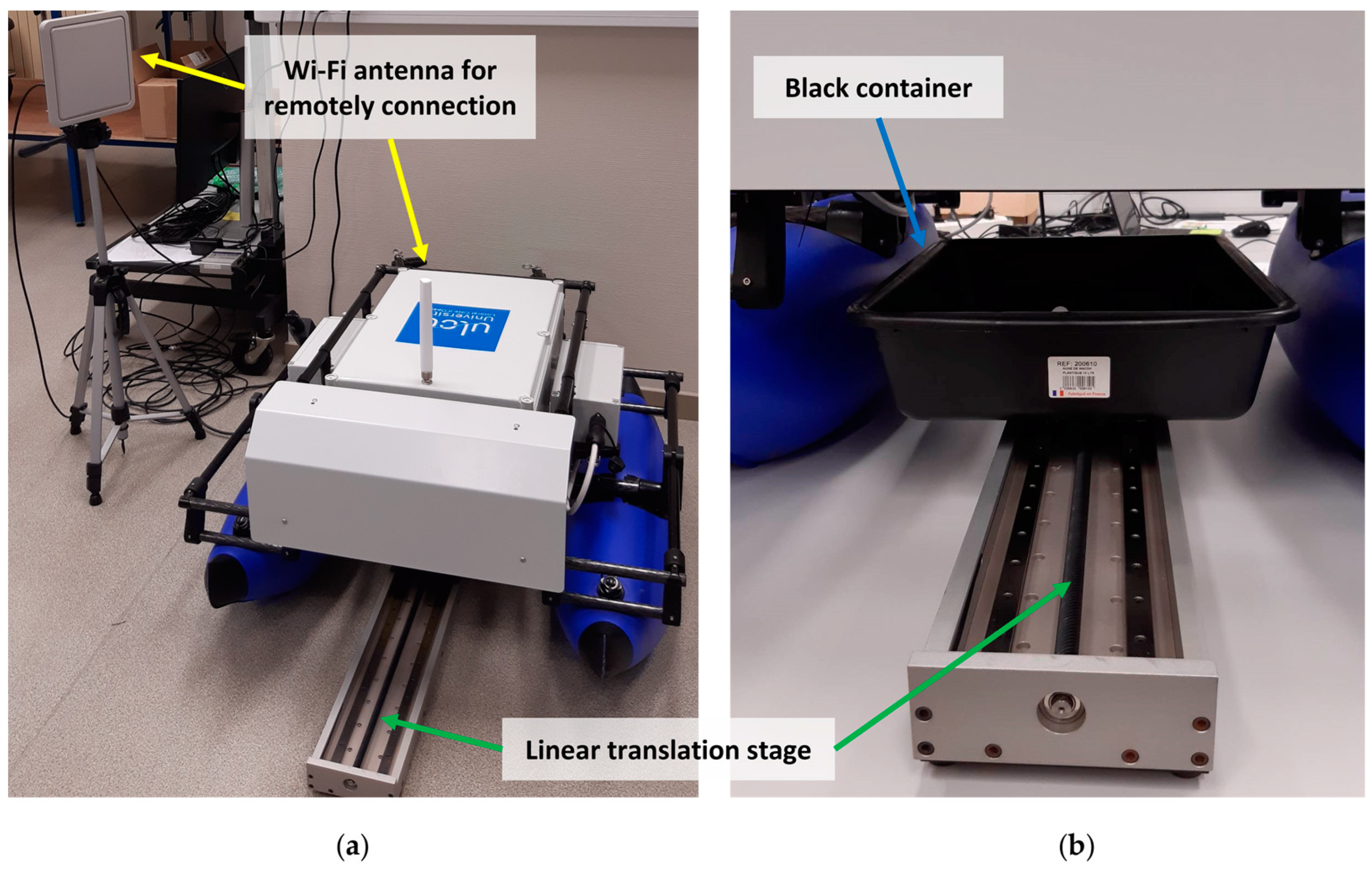
To simulate an aquatic environment, a black PVC plastic container (dimensions of 45 × 32 × 10 cm³) was filled with clear seawater. Such a black container was used to hold the seawater and the objects because it has negligible reflectance values compared to the reflectance values of the observed objects over the NIR-SWIR spectrum, while water absorbs infrared light. The hyperspectral camera was positioned at 45 cm of the water surface level to reproduce similar conditions to the real situation where the RHIS works on the water surface to detect the plastic type of the floating objects. For the linear motion simulation, a linear translation stage (linear scanner) was used to move the black container (Figure 4).

An embedded computer with the Spectronon Pro software was used to calibrate the camera, focus the objective lens, capture the hyperspectral data cubes, control the integration time and the frame rate of the camera, and drive the motor for the linear scanner. Although hyperspectral cameras are spectrally calibrated, they usually provide raw data, which need to be calibrated to obtain the absolute reflectance of the scanned objects. For this purpose, both the instrument sensor response and illumination functions were considered to correct the acquired images. This calibration, also named flat field correction, was, thus, performed by a dark correction followed by a response correction. For the dark correction, the dark reference was captured by completely closing the aperture of the camera, leading to no light striking the sensor, resulting in a true dark reflectance. For the response correction, a Spectralon^® white diffuse reflectance standard was used as a white reference with a reflectivity of 1 in all the wavelengths. The integration time was adjusted to maximize the apparent reflectance of the Spectralon calibration panel. For all acquisitions, the camera parameters were fixed so that the frame rate supported the integration time required for the illumination and sample brightness, as follows:

• Integration time: t_i = 2.049 ms;
• Frame rate: F = 22 fps (frames per second).

The speed of the linear translation stage was then adjusted to maintain a unity aspect ratio so that the observed objects were not distorted in the acquired images. We obtained hyperspectral images with the spatial resolution given by the ratio between the line of view length and the camera resolution.

Although the hyperspectral camera Resonon PIKA-NIR320 covers the spectral range from 900 to 1700 nm with 168 spectral bands, the 13 first spectral bands and the 12 last spectral bands provide too noisy and distorted information to be exploited. For this reason, these 25 spectral bands were neglected by reducing the number of bands from 168 to 143, with an interval of the wavelength from 949.2 nm to 1650.8 nm instead of the real interval of the wavelength from 886.3 nm to 1711.4 nm.

This setup was used to acquire hyperspectral images of different waste samples in order to spectrally characterize them, compare their spectrum with the state-of-the-art to validate the proposed RHIS, on the one hand, and prove the RHIS’s ability to recognize the different plastic litter, on the other hand. The database built for this purpose is presented in the next subsection.

2.3. Benchmark Image Database

In our study, plastic waste samples were collected from estuarine and coastal beaches along the Eastern English Channel French coast. In addition, some virgin plastics were used to expand the plastic library, which led to a set of plastic objects that contained and represented all plastic types. A categorized overview of these plastics objects and their types is shown in

Table 1. Examples of waste samples for each plastic type.

Number of Objects	Plastic Type
19	HDPE	Yellow rope	White plastic bag	Green net rope	Yogurt cover
5	LDPE	Blue toothpaste tube	White toothpaste tube	Orange rope	Red water bottle neck
3	PET	Green bottle bottom	Transparent tomato packaging
23	PP	Red rope	Dark blue rope	Blue deodorant cover	Red cap
2	PVC	Black container	Semi-transparent packaging
2	PS	Pink cap parfum	White part of yogurt (yogurt box)
2	PUR	Gray fragment of pristine plastic	Gray fragment
1	POM	White fragment of pristine plastic
1	ABS	White fragment of pristine plastic

. They were divided into the following categories: (1) HDPE, (2) LDPE, (3) PET, (4) PP, (5) PVC, (6) PS, (7) PolyURethane (PUR), (8) PolyOxyMethylene (POM), (9) and ABS. A tenth category of non-plastic materials found in the aquatic environment (wood, vegetation, cardboard, clear seawater, etc.) and named “Other” was also added. We can notice in Table 1 that the number of objects was different depending on the plastic type. This variation was representative of the diversity of products made with each type of plastic.

The polymer that constituted each type of plastic object presented in Table 1 was then identified by a Macro-Raman Spectrometer (MacroRAM, Horiba Scientific, France, Palaiseau) using a laser of a 785 nm wavelength with a power of 7–450 mW and a fixed grating of 685 gr.mm⁻¹ with a spectral range from 100–3400 cm⁻¹ [26,27]. This spectrometer was equipped with a CCD detector for a spectral resolution of 8 cm⁻¹ at 914 nm. The signal acquisition and processing were realized with Labspec software and its identification using the KnowItAll software (KnowItAll, BioRad^®) and the free-access spectra libraries of Horiba (Raman-Forensic-Horiba) and SLoPP/SLoPP-E. These identifications served as a ground-truth to label the data of our benchmark waste hyperspectral image database.

To create a hyperspectral image database of real marine litter, we performed 39 acquisitions with all the plastic objects presented in Table 1 under several positions using the RHIS in a controlled environment. Similar to [28], two cases were studied: dry and wet objects. The same object was scanned three times under several positions (face up or face down, side up or side down, etc.) and different views of its presence as an object floating (dry and wet) on seawater. We, thus, obtained a database of hyperspectral images which contained hyperspectral data cubes of the nine plastic types (HDPE, LDPE, PET, PP, PVC, PS, PUR, POM, ABS) and the “Other” category.

Two different datasets were then derived from this benchmark image database in order to carry out the two experiments presented in Section 3 and Section 4, respectively. The first dataset consisted of reference mean hyperspectral reflectance spectra, and it was used to perform a spectral data analysis (Section 3). The second dataset was a labeled waste image patch dataset, which was used to assess the classification performance of the proposed system (Section 4).

3. Spectral Data Analysis

This section presents an in situ spectral analysis conducted with the proposed RHIS in order to characterize the hyperspectral reflectance of plastic litter samples (Section 3.1). This analysis aimed to demonstrate that the obtained spectral reflectance of each plastic type was similar to those existing in the literature and, thus, confirm which wavelengths were most-efficient in discriminating between plastic types (Section 3.2).

3.1. Spectral Reflectance Dataset

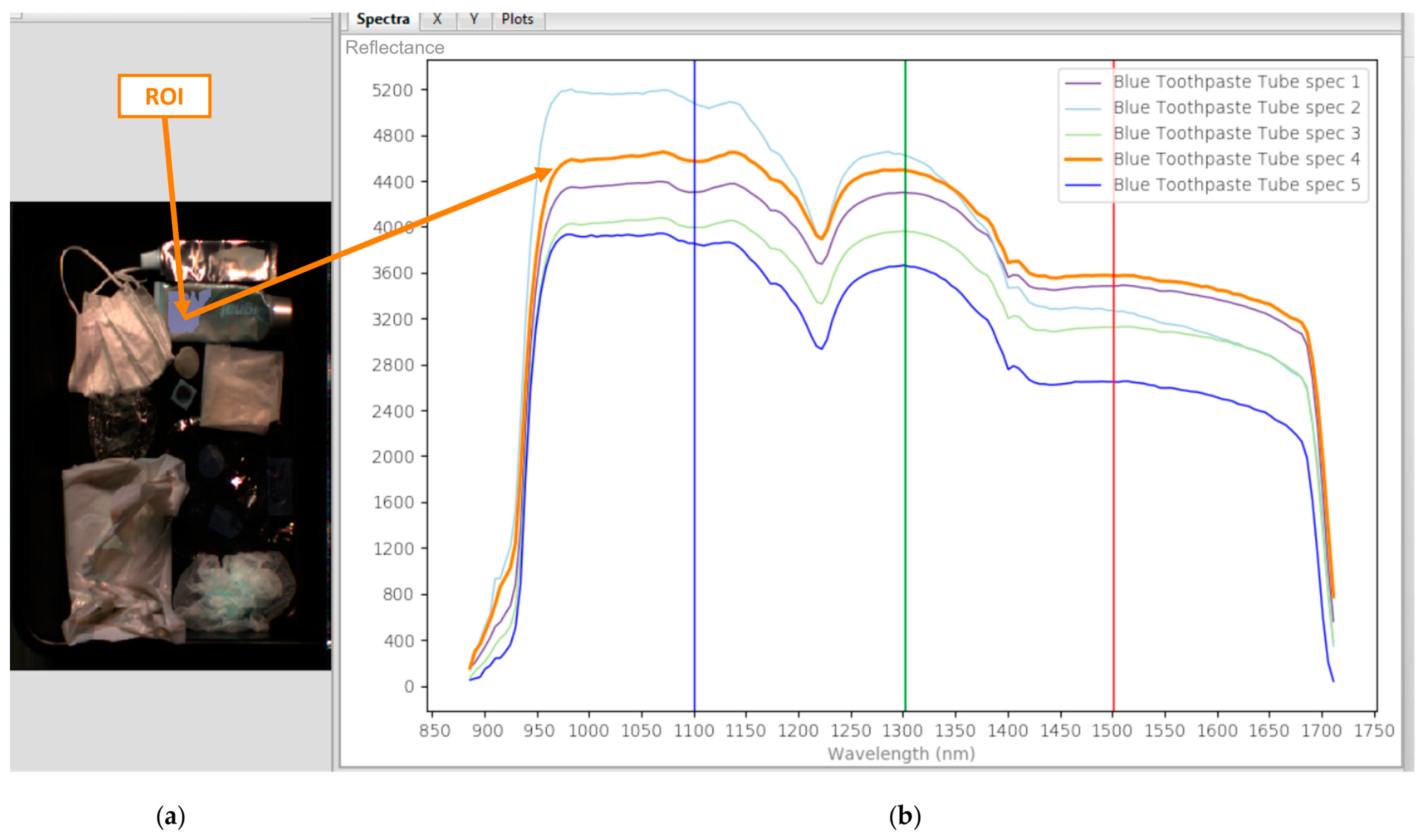
Using the new RHIS and Spectronon Pro software, the reflectance spectra were defined as references to characterize and verify the spectral reflectance of each object category. For this purpose, each hyperspectral data cube image was visualized (Figure 5) and different Regions Of Interest (ROIs) were then selected with various sizes and numbers depending on the size of each object. Large-area objects allowed selecting a large size and/or a large number of ROIs, while small-area objects limited the size and/or the number of ROIs. Each ROI was labeled by its type of plastic or Other.

For each waste sample presented in Table 1, the following steps were applied:

• Manual selection of a Region Of Interest (ROI) with a random size;
• Computation and plotting of the hyperspectral reflectance spectrum of the selected ROI as the mean value over all pixels in the ROI;
• Choice of another ROI of the same object present in another acquisition;
• Return to Step 2, and repeat this process until a significative number of spectra are computed depending on the size of the object.

All selected ROIs represented two possible cases (dry and wet) of the plastic object in seawater.

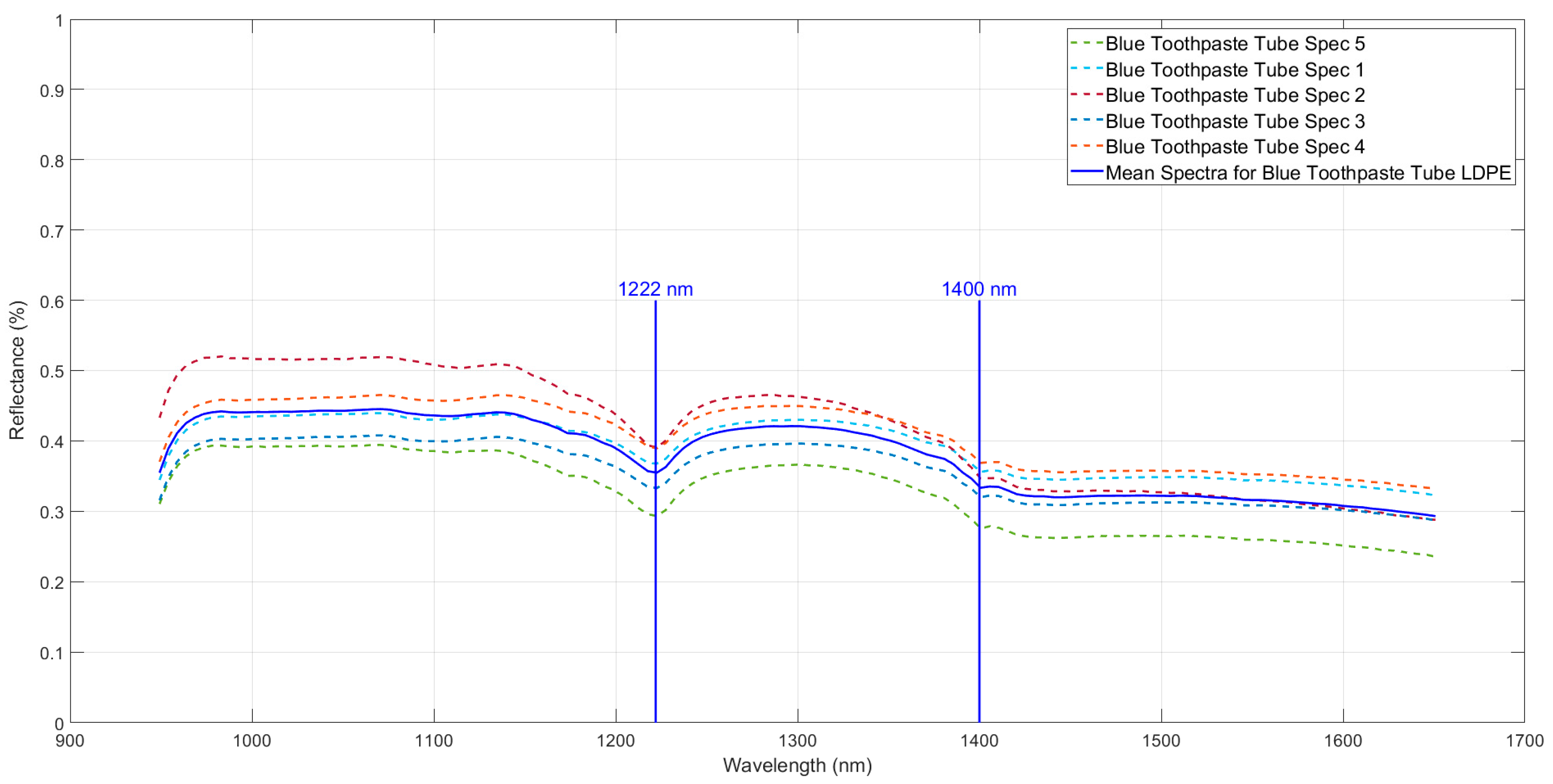
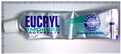
For example, Figure 5 shows each of the hyperspectral reflectance spectra computed from five ROI extracted from the LDPE plastic object “Blue toothpaste tube”.

The so-computed spectral data were quantized by an integer whose maximum value depended on the bit depth. Each hyperspectral reflectance spectrum was then normalized by using the reflectance factor given for each acquisition so that all the reflectance values belonged to the interval [0, 1]. Finally, a reference mean hyperspectral reflectance spectrum of each plastic object was calculated as the average of the normalized mean hyperspectral reflectance spectra of the selected ROIs from this object.

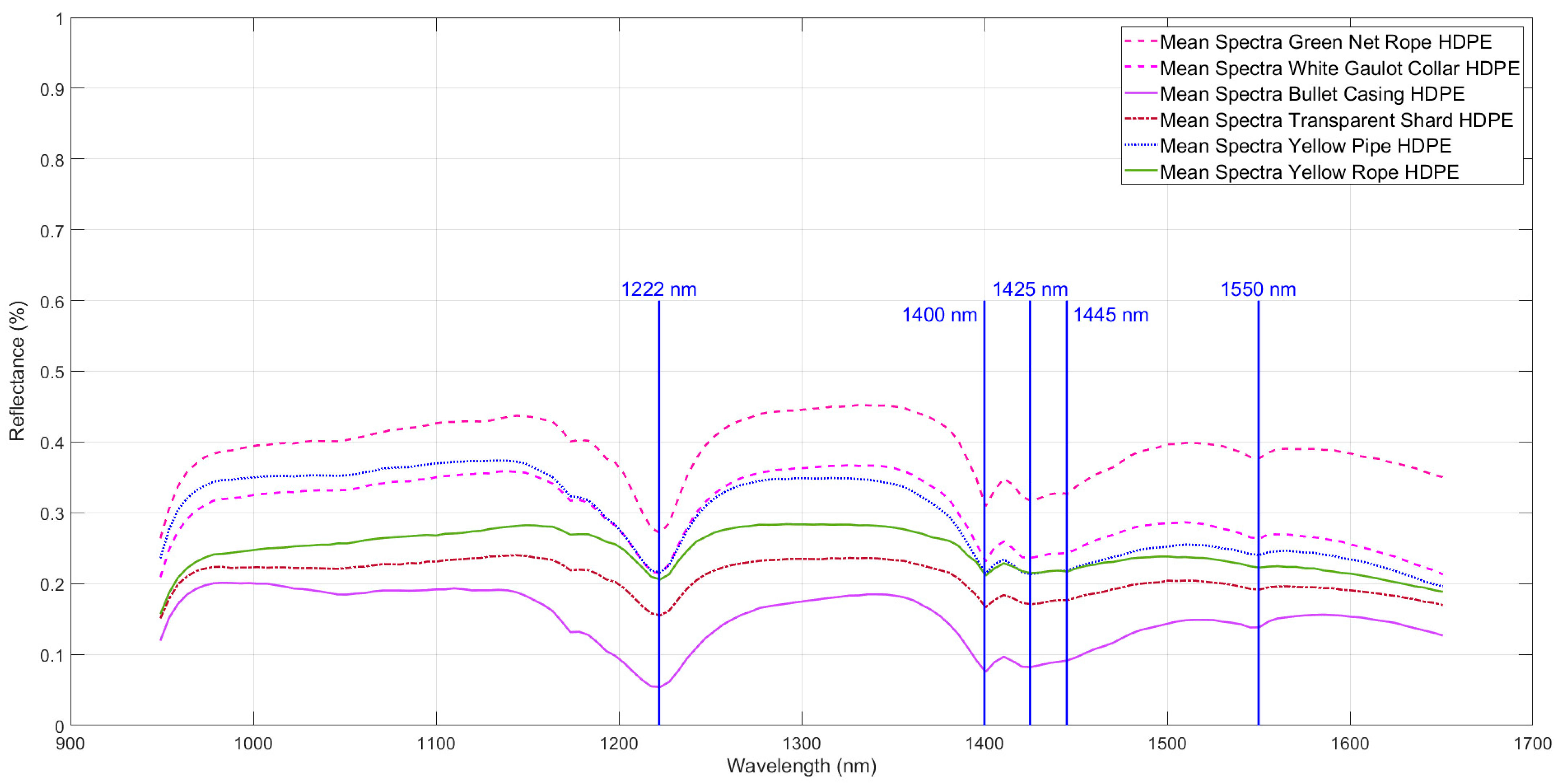
For example, Figure 6 displays the reference mean hyperspectral reflectance spectrum (called mean spectra) of the LDPE plastic object “Blue Toothpaste Tube” in the case where it was dry. This figure shows that the different spectra of the same object were close to each other and its reference mean hyperspectral reflectance spectrum can be used as a spectral signature of the type of plastic. Figure 7 displays the reference mean hyperspectral reflectance spectra of different dry objects (green net rope, yellow rope, etc.) of the same plastic type HDPE. This figure shows that the shape of the different spectra was similar with the absorption features located at the same wavelengths. The level of each spectrum along the reflectance axis can vary depending on the color and opacity of the plastic under consideration.

Finally, a dataset of 382 reference mean hyperspectral reflectance spectra was computed (104 for HDPE; 26 for LDPE, 34 for PET, 129 for PP, 18 for PVC, 22 for PS, 13 for PUR, 4 for POM, 9 for ABS, 23 for Other). An overview of this dataset can be found in the Supplementary Materials (Spreadsheet S1).

3.2. Comparison with the State-of-the-Art

In this section, the reference mean hyperspectral reflectance spectra presented in Section 3.1 are analyzed to identify the absorption feature wavelengths for each type of plastic and are compared to those of the literature.

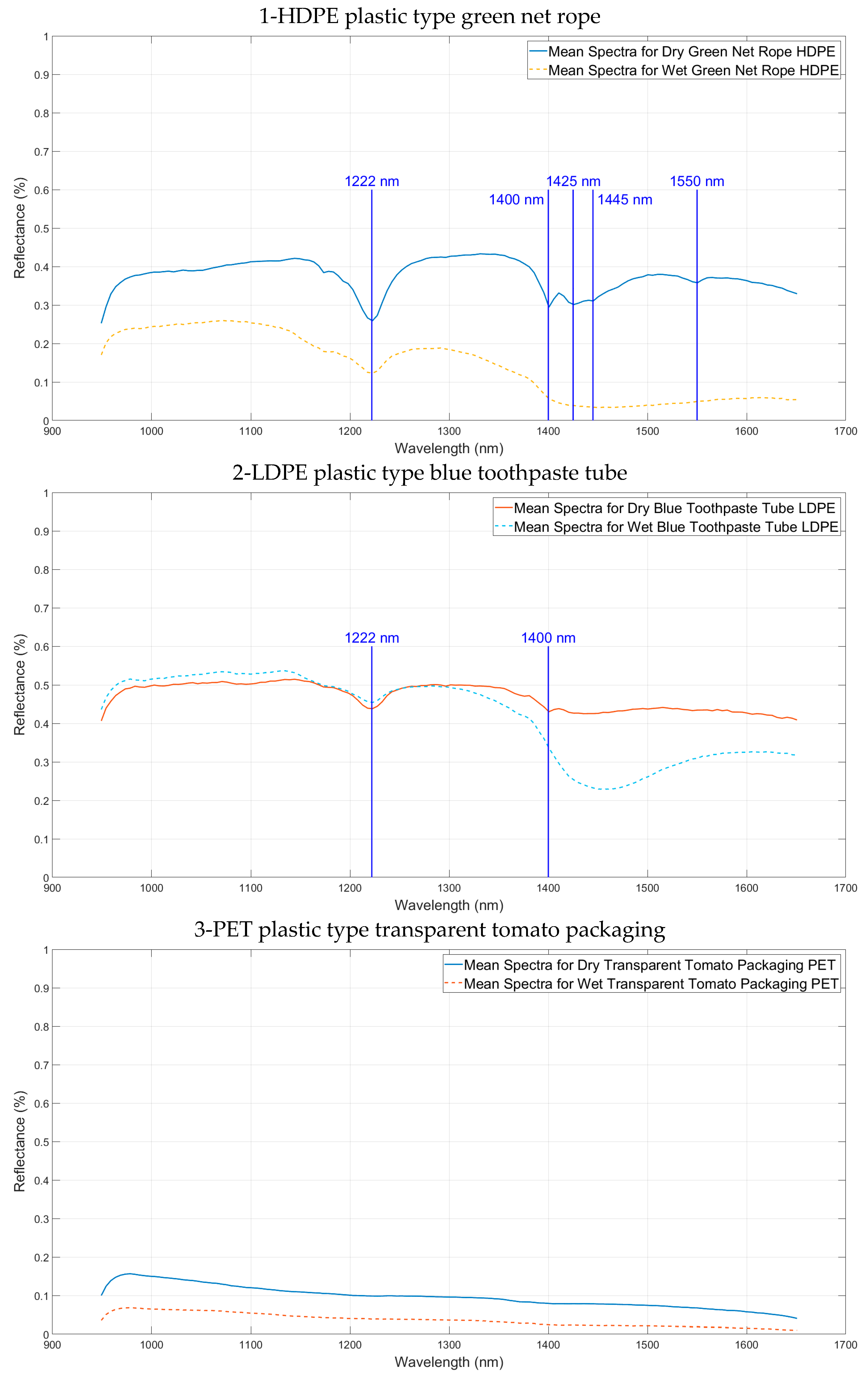
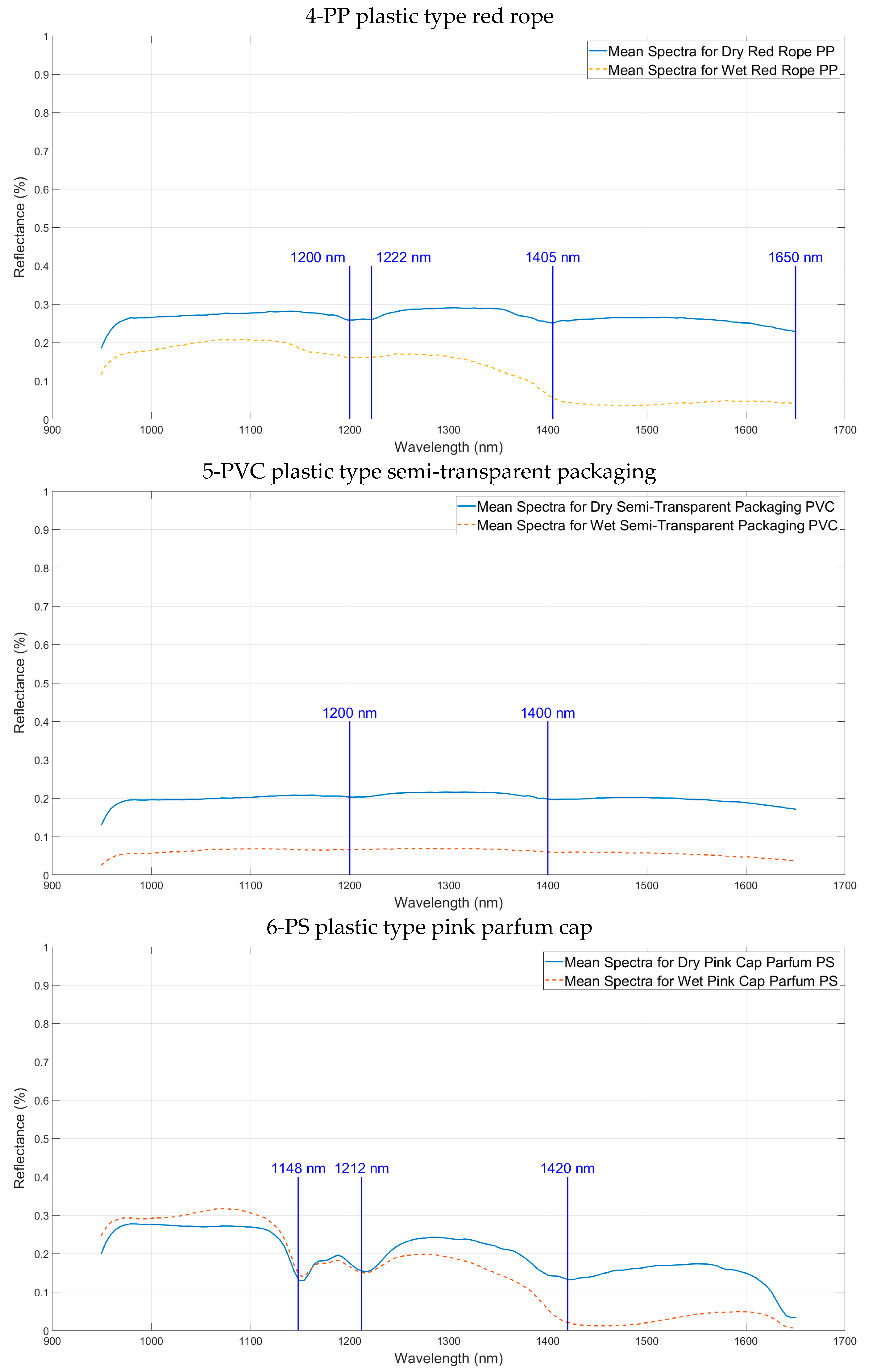
Figure 8 and Figure 9 present the reflectance spectra of six objects whose plastic type was HDPE, LDPE, PET, PP, PVC, and PS, respectively. Two spectra are presented for each object depending on whether it was dry or wet. In each case, the absorption feature wavelengths identified in the literature are highlighted in blue to be compared to our reflectance spectra. The objects analyzed in this study are listed below:

• HDPE plastic type—green net rope: The dry HDPE had five visible absorption features at wavelengths of 1222 nm, 1400 nm, 1425 nm, 1445 nm, and 1550 nm [3,8]. The most-important absorption feature is at a wavelength of 1222 nm, which is in close correspondence with the work of Tasseron et al. [3]. Similar results also appear in Figure 7 for dry objects. The wet green net rope of the HDPE plastic type had an attenuated spectral reflectance. However, the main absorption feature (1222 nm) remained visible.
• LDPE plastic type—blue toothpaste tube: The dry LDPE plastic had two absorption features at wavelengths of 1222 nm and 1400 nm, which is in close correspondence with Tasseron et al. [3]. Similar results also appear in Figure 6 for dry objects. The reflectance spectrum of the wet blue toothpaste tube of LDPE plastic was also attenuated. The two main absorption features of polyethene plastics (HDPE and LDPE) found in this study were centered on wavelengths of 1222 nm and 1400 nm, which is very similar to the absorption features described by Tasseron et al. [3].
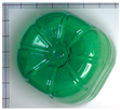
• PET plastic type—transparent tomato packaging: The dry PET spectral reflectance decreased with increasing wavelengths. The wet semi-transparent packaging of PET plastic type had an attenuated reflectance spectrum. The spectral shape of the transparent PET type found by Tasseron et al. [3] was similar to the spectral shape found in this study. No absorption feature can be highlighted for this type of plastic, whose reflectance was further reduced due to the transparency of the object, which reflected a small amount of light.
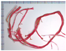
• PP plastic type—red rope: The dry PP had four visible absorption features at wavelengths of 1200 nm, 1222 nm, 1405 nm, and 1650 nm. The most-important absorption features were usually at wavelengths of 1222 nm, 1405 nm, and 1650 nm. The absorption features of PPplastics found in this study were centered on wavelengths of 1222 nm and 1405 nm, which is in close correspondence with Tasseron et al. [3] and Moshtaghi et al. [6]. The wet red rope plastic of the PP plastic type had an attenuated reflectance spectrum.
• PVC plastic type—semi-transparent packaging: The dry PVC had two small absorption features at wavelengths of 1200–1202 nm and 1400–1405 nm. The wet semi-transparent packaging of the PVC plastic type had an attenuated reflectance spectra, but it was similar to the dry spectra. The transparency of this object generated low-level spectra along the reflectance axis since the light rays were transmitted through the material to be partly absorbed by the water. Although this specific type of plastic packaging tends to float on water, other PVC objects are rarely found floating due to the high density of this polymer relative to water and was, therefore, not considered by Tasseron et al. [3].
• PS plastic type—pink parfum cap: The dry PS had three important absorption features at wavelengths of 1148 nm, 1212 nm, and 1420 nm. The wet pink parfum cap of the PS plastic type had an attenuated reflectance spectrum. Polystyrene was characterized by two distinct absorption features at 1150 and 1450 nm by Tasseron et al. [3].

This study using the new RHIS revealed the presence of absorption features in the reference mean hyperspectral reflectance spectra of different plastic types in the NIR–SWIR range centered on wavelengths of: 1148 nm, 1200 nm, 1212 nm, 1222 nm, 1400 nm, 1405 nm, 1420 nm, 1425 nm, 1445 nm, 1550 nm, and 1650 nm. These results, which were in correspondence with the results obtained by Tasseron et al. [3] and Moshtaghi et al. [6], confirmed that the RHIS was able to characterize each plastic type by a spectral signature.

4. Plastic Litter Recognition Using Machine Learning

This section aims to show that the new RHIS is able to automatically recognize the plastic type of the observed objects by hyperspectral image analysis. To evaluate the recognition performances, it was necessary to dispose of a ground-truth where the category of each analyzed data is known. From the benchmark database presented in Section 2.3, a dataset of image patches was, thus, built, where each patch was labeled by a class of plastic or other (Section 4.1). This dataset was then used to apply classical supervised machine learning methods in order to classify the images of waste samples (Section 4.2).

All calculations were performed with Matlab^® R2021b and a Windows 10TM computer with an Intel(R) Core(TM) i9-9880H CPU with 2.30 GHz, 32 GB RAM, and an Nvidia^® Quadro RTX 3000 graphics card with 16 GB GDDR5X memory.

4.1. Waste Image Patch Dataset

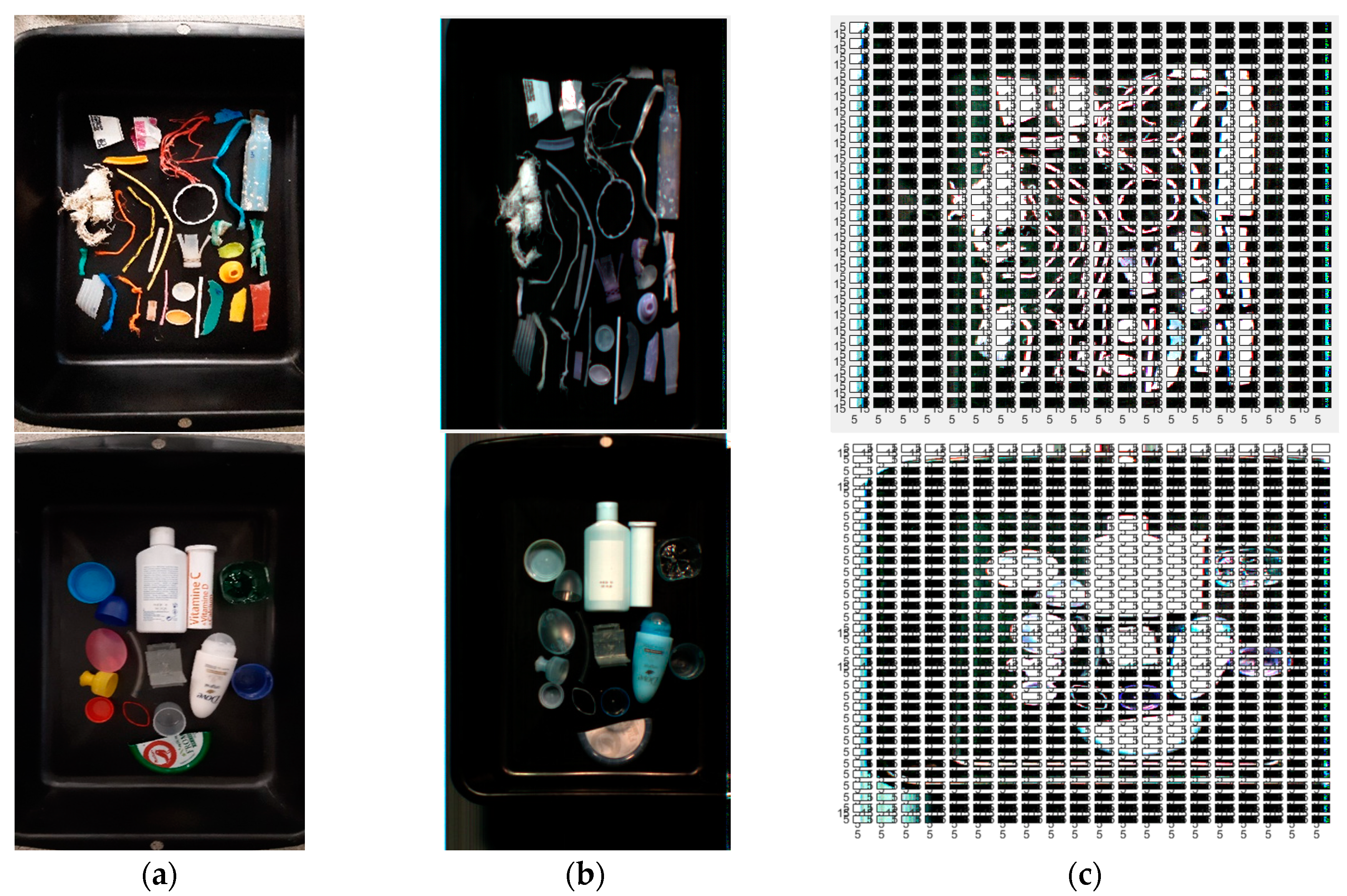
To build the waste image patch dataset, hyperspectral data cubes were extracted from the benchmark image database presented in Section 2.3. Manually labelling all the pixels of these images was a laborious task, which was not easily feasible. Each hyperspectral data cube was, therefore, divided into patches of size 16 × 16 × 143. The small size of certain plastic objects (Figure 10) led us to choose this patch size. Representative patches of each type of waste were then manually selected from different objects present in the images. Each selected patch was finally manually labeled according to its class, namely its type of plastic or other.

In order to assess the machine learning model performances, two subsets of image patches representative of the ten classes were created: a training subset for the model learning and a testing subset for the model evaluation. The training and testing image patches were extracted from different original images so that they were as independent as possible and represented a realistic situation in seawater with all its challenges.

For the training and the testing subsets, a total of 788 and 312 image patches of size 16 × 16 × 143 were, respectively, selected from the images of the benchmark database.

Table 2. Plastic type and “other” classes with the number of used patches for the training and testing image patch subsets.

Nine Plastic Types and “Other” (10 Classes)	Training Subsets Number of Patches	Testing Subsets Number of Patches
(1) HDPE	135	50
(2) LDPE	67	37
(3) PET	85	61
(4) PP	96	36
(5) PVC	236	55
(6) PS	4	2
(7) PUR	14	11
(8) POM	2	3
(9) ABS	6	3
(10) Other	143	54
Total Number of Patches	788	312

shows, in the first column, the different considered classes (nine plastic types and one class “other”). The number of patches that were used for training and testing are shown in the second and third column, respectively. This number depended on the number and size of the available objects for each type of plastic.

An overview of the representative patches counted per plastic object can be found in the Supplementary Materials (File S1).

4.2. Waste Image Patch Classification

In this section, three well-known supervised machine learning methods are applied to classify the image patches of the dataset presented in the previous section.

As can be observed in Table 2, the number of examples for each class varied. Some classes were represented with a small number of samples for classification, and the difference between the number of patches for the plastic types PUR, POM, PS, and ABS, and the Other types was significant. A class imbalance usually makes it harder to identify (and, hence, classify) a minority class. In our case, the plastic types of PUR, POM, PS, and ABS were minority classes. Imbalanced classification is a challenge for predictive modeling because most machine learning algorithms used for classification are designed around the assumption of an equal number of examples for each class. To take these limitations into account, three classical supervised machine learning methods were chosen:

• K-Nearest Neighbor classification (KNN) [29];
• Support Vector Machine (SVM) [30];
• Artificial Neural Network (ANN) [22,31,32,33].

For each method, there are parameters to be optimized to determine the best tuning of the classification model (classifier) by using the training image patches (learning stage) and then to evaluate its performance with the testing image patches (prediction stage). To fine-tune the classifier parameters with the challenge of class imbalance, Hyper-Parameter (HP) optimization methods (Bayesian [34,35] and random research [36]) offer the possibility to automatically select a classification model with an optimized tuning.

For these experiments, the mean hyperspectral reflectance associated with each patch of size (16 × 16 × 143) was calculated as the mean value over all its 256 (16 × 16) pixels, leading to a vector of size 1 × 143 (number of spectral bands).

In this study, high-definition hyperspectral images were used to classify patches according to different plastic types. However, the high dimension of hyperspectral images often causes computational complexity and the curse of dimensionality. In many cases, it is not necessary to process the hyperspectral information of all spectral bands since many spectral bands are highly correlated. Thus, it is required to remove redundant spectral bands in order to decrease the computational complexity and improve classification performance. Among the many dimensionality reduction methods used for this purpose, Principal Component Analysis (PCA) is a well-known preprocessing step in hyperspectral image analysis [37,38]. PCA linearly transforms the initial feature space, whose axes correspond to the input spectral bands, and generates a new feature subspace, where the axes are called principal components, in order to remove redundant dimensions.

The main following stages are, therefore, proposed for the plastic classification:

• Dimensionality reduction by feature extraction [38]: PCA was applied on the training subset, and different dimensions of the resulting feature subspace were considered for the next stage.
• Learning stage: The KNN, SVM, and ANN classification models were applied with optimization methods (Bayesian and random research) of hyper-parameter tuning to determine the best validation accuracy. In order to protect against overfitting, a five-fold cross-validation was considered. This scheme partitions the training subset into five disjoint folds. Each fold was used once as a validation fold, and the others formed a set of training folds. For each validation fold, the classification model was trained using the training folds, and the classification accuracy was assessed using the validation fold. The average accuracy was then calculated over all the folds and was used to optimize the tunning of the classification model parameters. These hyper-parameters, which are presented in

  Table 3. Hyper-parameter search range of the supervised machine learning methods (KNN, SVM, and ANN) available with Matlab (Hyperparameter Optimization in Classification Learner App: MATLAB and Simulink (mathworks.com): https://www.mathworks.com/help/stats/hyperparameter-optimization-in-classification-learner-app.html, accessed on 28 March 2023).

  Supervised Machine Learning Model	Hyper-Parameter Search Range
  K-Nearest Neighbor classification (KNN)	Number of neighbors: 1–394	Distance metric: city block, Chebyshev, correlation, cosine, Euclidean, Hamming, Jaccard, Mahalanobis, Minkowski (cubic), Spearman	Distance weight: equal, inverse, squared inverse	Standardized data: yes, no
  Support Vector Machine (SVM)	Multiclass method: one-vs.-all, one-vs.-one	Box constraint level: 0.001–1000	Kernel scale: 0.001–1000 Kernel function: Gaussian, linear, quadratic, cubic	Standardized data: yes, no
  Artificial Neural Network (ANN)	Number of fully connected layers: 1–3	Activation: ReLU, tanh, sigmoid, none	Regularization strength (Lambda): 1.269 × 10−8–126.9036	Standardized data: Yes, No
  	First layer size: 1–300	Second layer size: 1–300	Third layer size: 1–300	Iteration limit: 1–1000

  , were determined by an automatic hyper-parameter optimization using two methods: Bayesian [34,35] and random research [36] optimization. The final validation accuracy gave a good estimate of the predictive accuracy of the classifier, which was used in the next stage with the full training subset, excluding any data reserved for the testing subset.
• Prediction stage: The trained models obtained during the previous stage were then applied to the testing image patches, and the overall test accuracy of the classifier was determined. The testing subset here was independent of the training subset.

Based on these stages,

Table 4. The top ten classifiers and their determined optimized hyper-parameters.

Classification Models		PCA Values	Optimizer Options	Fine-Tuning/Optimized Hyper-Parameters				Validation Accuracy	Test Accuracy
KNN				Number of neighbors	Distance metric	Distance weight	Standardized data
	Model1- KNN	PCA disabled	Random search	1	Correlation	Inverse	true	89.2%	73.1%
	Model2-PCA48-KNN	48	Random search	5	Spearman	Inverse	false	89.7%	89.1%
	Model3-PCA48-KNN	48	Bayesian optimization	2	Spearman	Squared inverse	false	91.0%	85.3%
	Model4-PCA64-KNN	64	Random search	10	Spearman	Squared inverse	false	90.2%	87.8%
	Model5-PCA64-KNN	64	Bayesian optimization	2	Spearman	Equal	false	92.1%	87.2%
	Model6- PCA96-KNN	96	Random search	1	Spearman	Squared inverse	false	90.7%	86.9%
SVM (kernel scale: 1)				Multiclass method	Box constraint level	Kernel function	Standardized data
	Model7- PCA64-SVM	64	Bayesian optimization	One-vs.-all	627.1421	Quadratic	false	88.6%	85.3%
	Model8- PCA64-SVM	64	Random search	One-vs.-all	268.3711	Cubic	false	88.5%	72.8%
Neural Network ANN	Model9- PCA64-ANN	64	Bayesian optimization	Number of fully connected layers: 1	Activation: none	Regularization strength (Lambda): 5.0497 × 10−8	Standardized data: No	87.6%	71.8%
				First layer size: 19	Second layer size: 0	Third layer size: 0	Iteration limit: 1000
	Model10-PCA64-ANN	48	Random search	Number of fully connected layers: 2	Activation: tanh	Regularization strength (Lambda): 7.8208 × 10−7	Standardized data: No	87.9%	84.6%
				First layer size: 17	Second layer size: 288	Third layer size: 0	Iteration limit: 1000

presents the top ten classifiers that were tested with different dimensions of the feature subspace obtained by PCA (96, 64, and 48) and with the two HP optimization methods. The first column of this table gives the name of the tested classifier; the second one indicates the dimension of the feature subspace; the third column gives the name of the used HP optimization method. The goal of the optimization algorithm is to find a combination of HP values that minimizes an objective function, here the classification error rate. To find this combination, the iteration number of the used algorithm was fixed to 120. Table 4 also describes the determined optimized hyper-parameters in the fourth column. This column is divided into several cells, whose number depends on the classification method. For each tested classifier, the validation accuracy computed with the training subset and the test accuracy computed with the testing subset appear in the fifth and sixth columns, respectively. Accuracy is given as the percentage of patches (training or testing) that were correctly classified.

Table 4 first shows that the KNN classification model outperformed the SVM and ANN ones in terms of validation accuracy and test accuracy. This table also shows that, for the KNN model, PCA drastically increased the test accuracy. The KNN model with the highest test accuracy (89.1 %) was Model2-PCA48-KNN, which uses the 48 principal components of PCA. The optimized HP were determined with a random search method. Although the validation accuracy was not the highest for this classifier (89.7 %), it was very close to the test accuracy despite the imbalanced classification problem. This result showed that the validation accuracy provided a good estimate for the model performance on new data compared to the training data. The top validation accuracy was obtained with Model5-PCA64-KNN, which uses the 64 principal components of PCA, but this classifier achieved a test accuracy of 87.2% and, therefore, gave a lower performance.

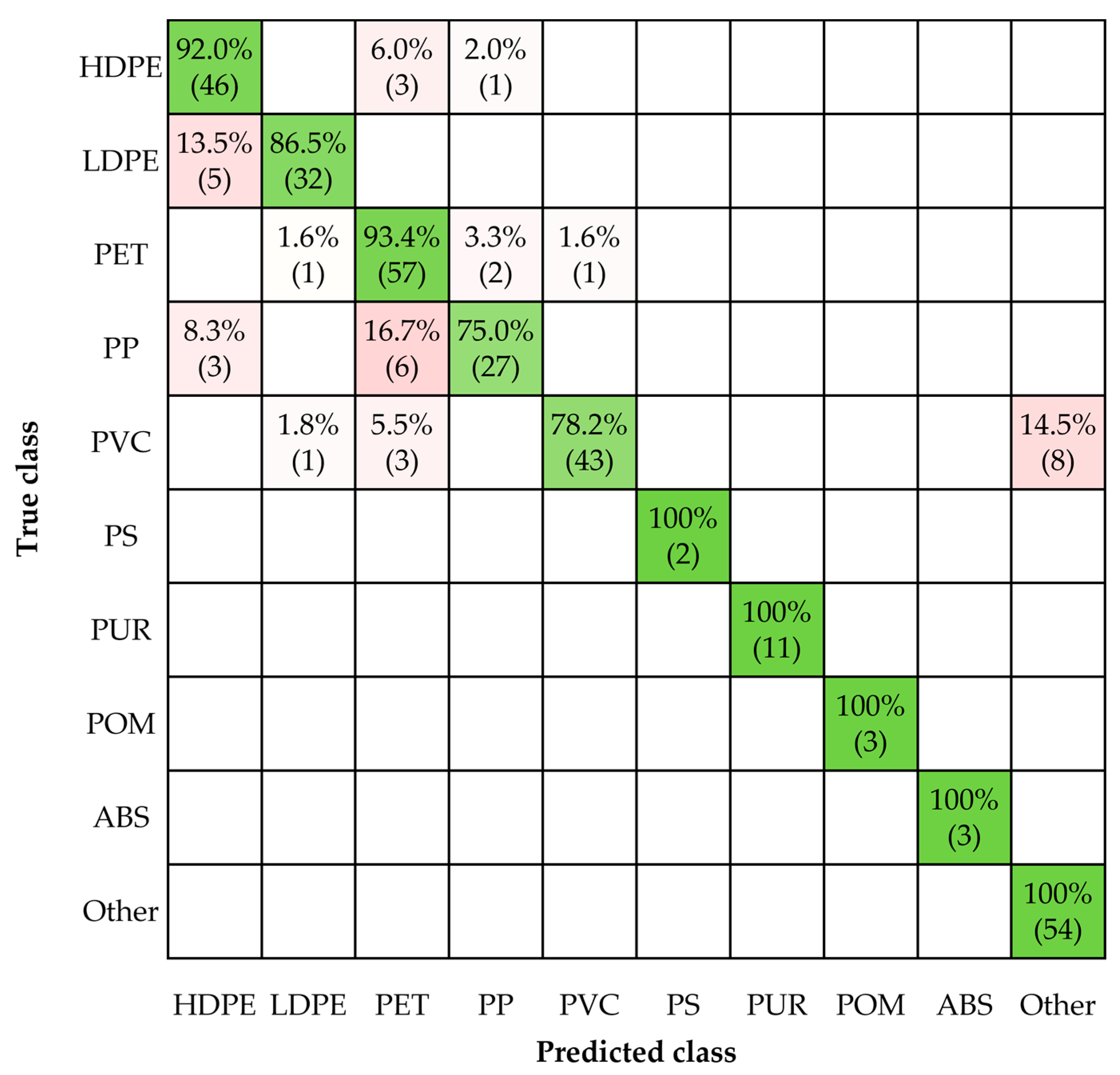
Figure 11 gives the test confusion matrix, which details the performances per class obtained for Model2-PCA48-KNN on the testing subset. Its rows correspond to the predicted class and its columns to the true class. The diagonal cells correspond to patches that were correctly classified, and the off-diagonal cells correspond to incorrectly classified patches. Both the percentage of patches and the number of patches (in brackets) are shown in each cell. This matrix shows that the testing patches corresponding to the four minority classes (PUR, POM, PS, and ABS) were well classified (100% of test accuracy) despite the imbalanced classification issue. The class of other materials that represents non-plastic objects corresponded also to 100% accuracy. This result proved that the classifier was able to predict whether an object was a plastic or not. The testing patches with the lowest accuracy belonged to the PP and PVC classes. There were 16.7% of PP samples assigned to the PET class and 8.3% to the HDPE class. There were 14.5% of PVC samples assigned to the class other. These misclassification rates could be explained by the presence of wet samples with distorted spectra, by the presence of transparent and black plastics with poor reflectance, and by the diversity of samples in the class Other. The HDPE and LDPE classes can be confused since 13.5% of the LDPE samples were assigned to the HDPE class. These two types of plastic are based on the same polymer. Finally, the accuracy obtained for each of the other class was greater than 90%, which is a very good performance with a classical classifier.

These experimental results highlighted that the RHIS provided a very satisfactory wet and dry plastic recognition performance by using classical supervised machine learning methods such as the Model2-PCA48-KNN classifier. With more training data and more sophisticated classification approaches such as deep learning approaches, this performance can obviously be further improved for the detection and identification of plastic litter [22,30].

The RHIS is the first embedded hyperspectral imaging system that observes the aquatic environment in the near-field and automatically quantifies and qualifies polymers of floating plastic litter with accuracy.

5. Conclusions

This paper addressed the problem of plastic litter pollution in the aquatic environment resulting from human activity. The observation and quantification of this waste by remote sensing at different scales is crucial to determine its exact nature and fight against this pollution. Hyperspectral imaging is emerging as an appropriate technology to characterize, detect, and identify floated plastic waste in terms of shape and type of polymers. In this paper, a new remote hyperspectral imaging system, embedded on an unmanned aquatic drone for plastic detection and identification in coastal environment, was presented.

This new hyperspectral imaging system, named the ROV-ULCO, was designed around a hyperspectral camera that captures reflectance spectra in the NIR to SWIR range to discriminate different types of plastic. It works in the near-field for the observation of floating litter (plastic and non-plastic type). The first obtained results were very encouraging and proved the marine litter automatic recognition capability using a simple supervised machine learning method. Indeed, these results reached an overall accuracy close to 90% with a K-nearest neighbors classifier associated with a principal component analysis for the classification of nine plastic types and their distinction with a tenth class of non-plastic objects.

This study showed that the new hyperspectral imaging system, the ROV-ULCO, is a promising approach to detect and identify plastic waste in aquatic environments. It can be improved by focusing on challenges such as transparent and black plastic waste or wet and submerged plastic waste, which are more difficult to recognize [39]. From our perspective, the databases will be enlarged to add these plastic types with more representative samples, and classification approaches based on artificial intelligence will be applied in order to improve the performance of this original system. In addition, our prototype can be equipped with other optical or radar sensors to meet these challenges, but also to make it autonomous so that it can automatically navigate to areas where plastic waste is present.

References

1. Wolf, M.; Berg, K.V.D.; Garaba, S.P.; Gnann, N.; Sattler, K.; Stahl, F.; Zielinski, O. Machine learning for aquatic plastic litter detection, classification and quantification (APLASTIC-Q). Environ. Res. Lett. 2020, 15, 114042. [Google Scholar] [CrossRef]
2. Tasseron, P.F.; Schreyers, L.; Peller, J.; Biermann, L.; van Emmerik, T. Toward robust river plastic detection: Combining lab and field-based hyperspectral imagery. Earth Space Sci. 2022, 9, e2022EA002518. [Google Scholar] [CrossRef]
3. Tasseron, P.; van Emmerik, T.; Peller, J.; Schreyers, L.; Biermann, L. Advancing floating macroplastic detection from space using experimental hyperspectral imagery. Remote Sens. 2021, 13, 2335. [Google Scholar] [CrossRef]
4. Freitas, S.; Silva, H.; Silva, E. Remote hyperspectral imaging acquisition and characterization for marine litter detection. Remote Sens. 2021, 13, 2536. [Google Scholar] [CrossRef]
5. Zhou, S.; Kaufmann, H.; Bohn, N.; Bochow, M.; Kuester, T.; Segl, K. Identifying distinct plastics in hyperspectral experimental lab, aircraft-, and satellite data using machine/deep learning methods trained with synthetically mixed spectral data. Remote Sens. Environ. 2022, 281, 113263. [Google Scholar] [CrossRef]
6. Moshtaghi, M.; Knaeps, E.; Sterckx, S.; Garaba, S.; Meire, D. Spectral reflectance of marine macroplastics in the VNIR and SWIR measured in a controlled environment. Sci. Rep. 2021, 11, 5436. [Google Scholar] [CrossRef] [PubMed]
7. Mehrubeoglu, M.; Sickle, A.V.; Turner, J. Detection and identification of plastics using SWIR hyperspectral imaging. In Imaging Spectrometry XXIV: Applications, Sensors, and Processing; SPIE: Online Only, CA, USA, 2020; Volume 11504, p. 115040G. [Google Scholar] [CrossRef]
8. Cocking, J.; Narayanaswamy, B.E.; Waluda, C.M.; Williamson, B.J. Aerial detection of beached marine plastic using a novel, hyperspectral short-wave infrared (SWIR) camera. ICES J. Mar. Sci. 2022, 79, 648–660. [Google Scholar] [CrossRef]
9. Hu, C. Remote detection of marine debris using satellite observations in the visible and near infrared spectral range: Challenges and potentials. Remote Sens. Environ. 2021, 259, 112414. [Google Scholar] [CrossRef]
10. Balsi, M.; Moroni, M.; Chiarabini, V.; Tanda, G. High-resolution aerial detection of marine plastic litter by hyperspectral sensing. Remote Sens. 2021, 13, 1557. [Google Scholar] [CrossRef]
11. Leone, G.; Catarino, A.I.; Keukelaere, L.D.; Bossaer, M.; Knaeps, E.; Everaert, G. Hyperspectral reflectance dataset of pristine, weathered and biofouled plastics. Earth Syst. Sci. Data Discuss. 2022, 15, 745–752. [Google Scholar] [CrossRef]
12. Zhou, S.; Kuester, T.; Bochow, M.; Bohn, N.; Brell, M.; Kaufmann, H. A knowledge-based, validated classifier for the identification of aliphatic and aromatic plastics by WorldView-3 satellite data. Remote Sens. Environ. 2021, 264, 112598. [Google Scholar] [CrossRef]
13. Biermann, L.; Clewley, D.; Martinez-Vicente, V.; Topouzelis, K. Finding plastic patches in coastal waters using optical satellite data. Sci. Rep. 2020, 10, 2825–2830. [Google Scholar] [CrossRef] [PubMed] [Green Version]
14. Bentley, J. Detecting Ocean Microplastics with Remote Sensing in the Near-Infrared: A Feasibility Study. 2019. Available online: https://vc.bridgew.edu/cgi/viewcontent.cgi?article=1309&context=honors_proj (accessed on 28 March 2023).
15. Topouzelis, K.; Papageorgiou, D.; Karagaitanakis, A.; Papakonstantinou, A.; Ballesteros, M.A. Remote sensing of sea surface artificial floating plastic targets with Sentinel-2 and unmanned aerial systems (plastic litter project 2019). Remote Sens. 2020, 12, 2013. [Google Scholar] [CrossRef]
16. Bao, Z.; Sha, J.; Li, X.; Hanchiso, T.; Shifaw, E. Monitoring of beach litter by automatic interpretation of unmanned aerial vehicle images using the segmentation threshold method. Mar. Pollut. Bull. 2018, 137, 388–398. [Google Scholar] [CrossRef]
17. Topouzelis, K.; Papageorgiou, D.; Suaria, G.; Aliani, S. Floating marine litter detection algorithms and techniques using optical remote sensing data: A review. Mar. Pollut. Bull. 2021, 170, 112675. [Google Scholar] [CrossRef]
18. Ramavaram, H.R.; Kotichintala, S.; Naik, S.; Critchley-Marrows, J.; Isaiah, O.T.; Pittala, M.; Wan, S.; Irorere, D. Tracking Ocean Plastics Using Aerial and Space Borne Platforms: Overview of Techniques and Challenges. In Proceedings of the 69th International Astronautical Congress (IAC), IAC 2018 Congress Proceedings. Bremen, Germany, 1–5 October 2018. [Google Scholar]
19. Iordache, M.-D.; Keukelaere, L.D.; Moelans, R.; Landuyt, L.; Moshtaghi, M.; Corradi, P.; Knaeps, E. Targeting plastics: Machine learning applied to litter detection in aerial multispectral images. Remote Sens. 2022, 14, 5820. [Google Scholar] [CrossRef]
20. Andriolo, U.; Gonçalves, G.; Bessa, F.; Sobral, P. Mapping marine litter on coastal dunes with unmanned aerial systems: A showcase on the Atlantic Coast. Sci. Total Environ. 2020, 736, 139632. [Google Scholar] [CrossRef]
21. Geraeds, M.; van Emmerik, T.; de Vries, R.; bin Ab Razak, M.S. Riverine plastic litter monitoring using Unmanned Aerial Vehicles (UAVs). Remote Sens. 2019, 11, 2045. [Google Scholar] [CrossRef] [Green Version]
22. Freitas, S.; Silva, H.; Silva, E. Hyperspectral imaging zero-shot learning for remote marine litter detection and classification. Remote Sens. 2022, 14, 5516. [Google Scholar] [CrossRef]
23. Kikaki, K.; Kakogeorgiou, I.; Mikeli, P.; Raitsos, D.E.; Karantzalos, K. MARIDA: A benchmark for Marine Debris detection from Sentinel-2 remote sensing data. PLoS ONE 2022, 17, e0262247. [Google Scholar] [CrossRef]
24. Freitas, S.; Silva, H.; Almeida, C.; Viegas, D.; Amaral, A.; Santos, T.; Dias, A.; Jorge, P.A.S.; Pham, C.K.; Moutinho, J.; et al. Hyperspectral imaging system for marine litter detection. In Proceedings of the OCEANS 2021: San Diego—Porto, San Diego, CA, USA, 20–23 September 2021; IEEE: New York, NY, USA, 2021; pp. 1–6. [Google Scholar] [CrossRef]
25. Pasquier, G.; Doyen, P.; Carlesi, N.; Amara, R. An innovative approach for microplastic sampling in all surface water bodies using an aquatic drone. Heliyon 2022, 8, e11662. [Google Scholar] [CrossRef]
26. Driedger, A.; Dürr, H.; Mitchell, K.; Flannery, J.; Brancazi, E.; Cappellen, P.V. Plastic debris: Remote sensing and characterization data streams and micro-satellites reflected infrared spectroscopy raman spectroscopy great lakes marine debris network. Int. J. Remote Sens. Mar. Pollut. Bull. 2007, 22, 1. [Google Scholar]
27. Neo, E.R.K.; Yeo, Z.; Low, J.S.C.; Goodship, V.; Debattista, K. A review on chemometric techniques with infrared, Raman and laser-induced breakdown spectroscopy for sorting plastic waste in the recycling industry. Resour. Conserv. Recycl. 2022, 180, 106217. [Google Scholar] [CrossRef]
28. Garaba, S.P.; Harmel, T. Top-of-atmosphere hyper and multispectral signatures of submerged plastic litter with changing water clarity and depth. Opt. Express 2022, 30, 16553. [Google Scholar] [CrossRef]
29. Ma, L.; Crawford, M.M.; Tian, J. Local manifold learning-based k-nearest-neighbor for hyperspectral image classification. IEEE Trans. Geosci. Remote Sens. 2010, 48, 4099–4109. [Google Scholar] [CrossRef]
30. Melgani, F.; Bruzzone, L. Classification of hyperspectral remote sensing images with support vector machines. IEEE Trans. Geosci. Remote Sens. 2004, 42, 1778–1790. [Google Scholar] [CrossRef] [Green Version]
31. Gnann, N.; Björn, B.; Ternes, T.A. Close-range remote sensing-based detection and identification of macroplastics on water assisted by artificial intelligence: A review. Water Res. 2022, 222, 118902. [Google Scholar] [CrossRef]
32. Glorot, X.; Bengio, Y. Understanding the difficulty of training deep feedforward neural networks. In Proceedings of the Thirteenth International Conference on Artificial Intelligence and Statistics, Sardinia, Italy, 13–15 May 2010; pp. 249–256. Available online: http://proceedings.mlr.press/v9/glorot10a/glorot10a.pdf (accessed on 28 March 2023).
33. He, K.; Zhang, X.; Ren, S.; Sun, J. Delving deep into rectifiers: Surpassing human-level performance on imagenet classification. In Proceedings of the IEEE International Conference on Computer Vision, Santiago, Chile, 11–18 December 2015; pp. 1026–1034. [Google Scholar] [CrossRef] [Green Version]
34. Snoek, J.; Larochelle, H.; Adams, R.P. Practical bayesian optimization of machine learning algorithms. Adv. Neural Inf. Process. Syst. 2012, 25. Available online: https://arxiv.org/pdf/1206.2944 (accessed on 28 March 2023).
35. Gelbart, M.A.; Snoek, J.; Adams, R.P. Bayesian optimization with unknown constraints. arXiv 2014, arXiv:1403.5607. [Google Scholar]
36. Bergstra, J.; Bengio, Y. Random search for hyper-parameter optimization. J. Mach. Learn. Res. 2012, 13, 281–305. Available online: https://dl.acm.org/doi/pdf/10.5555/2188385.2188395 (accessed on 28 March 2023).
37. Jolliffe, I.T. Principal Component Analysis, 2nd ed.; Springer: New York, NY, USA, 2002. [Google Scholar]
38. Lapajne, J.; Knapič, M.; Žibrat, U. Comparison of selected dimensionality reduction methods for detection of root-knot nematode infestations in potato tubers using hyperspectral imaging. Sensors 2022, 22, 367. [Google Scholar] [CrossRef] [PubMed]
39. Fiore, L.; Serranti, S.; Mazziotti, C.; Riccardi, E.; Benzi, M.; Bonifazi, G. Classification and distribution of freshwater microplastics along the Italian Po river by hyperspectral imaging. Environ. Sci. Pollut. Res. 2022, 29, 48588–48606. [Google Scholar] [CrossRef] [PubMed]
Figure 1. Conceptual framework for remote marine litter detection from [22] with different remote devices (satellite, airborne, drone, etc.) and with the new system (ROV-ULCO) proposed in this paper.
Remotesensing 15 03455 g001
Figure 2. ROV-ULCO system: RHIS embedded on a UAD, namely the Jellyfishbot, which can be connected with a net to collect macroplastics or microplastics in different water surfaces.
Remotesensing 15 03455 g002
Figure 3. Parts of the new RHIS. (a) outside components; (b) inside components.
Remotesensing 15 03455 g003
Figure 4. Experimental setup of the new remote hyperspectral imaging system. (a) Hyperspectral camera setup in controlled laboratory environment with WiFi antenna; (b) black container under the RHIS on the linear translation stage.
Remotesensing 15 03455 g004
Figure 5. Examples of hyperspectral reflectance computed from five ROIs (Spec. 1 to 5) of the LDPE plastic object “Blue Toothpaste Tube”. (a) Extraction of a region of interest from a hyperspectral image represented in false color; (b) non-normalized mean hyperspectral reflectance of different ROIs (in orange, the mean spectral reflectance over all pixels of the selected ROI).
Remotesensing 15 03455 g005
Figure 6. Examples of the reference mean hyperspectral reflectance of the tube and the cap of the LDPE plastic object “Blue Toothpaste Tube”.
Remotesensing 15 03455 g006
Figure 7. Examples of the reference mean hyperspectral reflectance of different HDPE plastic objects.
Remotesensing 15 03455 g007
Figure 8. Mean hyperspectral reflectance of plastic objects (HDPE, LDPE, and PET) depending on whether they were dry or wet and their corresponding absorption features.
Remotesensing 15 03455 g008
Figure 9. Mean hyperspectral reflectance of plastic objects (PP, PVC, and PS) depending on whether they are dry or wet and their corresponding absorption features.
Remotesensing 15 03455 g009
Figure 10. Examples of RGB and hyperspectral images of plastic objects. (a) RGB image of plastic objects; (b) false color image using three spectral bands of wavelength values of 1575.4 nm, 1257.1 nm, and 1100.0 nm; (c) selection of the image patches.
Remotesensing 15 03455 g010
Figure 11. Test confusion matrix with the Model2-PCA48-KNN classifier (89.1% overall accuracy).
Remotesensing 15 03455 g011