Article

Rethinking Representation Learning-Based Hyperspectral Target Detection: A Hierarchical Representation Residual Feature-Based Method

1
School of Communication and Information Engineering, Chongqing University of Posts and Telecommunications, Chongqing 400065, China
2
College of Computer Science, Chongqing University, Chongqing 400044, China
3
College of Information Science and Engineering, Henan University of Technology, Zhengzhou 453000, China
4
School of Cyber Science and Engineering, Nanjing University of Science and Technology, Nanjing 210094, China
5
College of Computer Science and Technology, Chongqing University of Posts and Telecommunications, Chongqing 400065, China
*
Author to whom correspondence should be addressed.
Remote Sens. 2023, 15(14), 3608; https://doi.org/10.3390/rs15143608
Submission received: 5 June 2023 / Revised: 12 July 2023 / Accepted: 17 July 2023 / Published: 19 July 2023

Abstract

:
Representation learning-based hyperspectral target detection (HTD) methods generally follow a learning paradigm of single-layer or one-step representation residual learning and the target detection on original full spectral bands, which, in some cases, cannot accurately distinguish the target pixels from variable background pixels via one-round of the detection process. To alleviate the problem and make full use of the latent discriminate characteristics in different spectral bands and the representation residual, this paper proposes a level-wise band-partition-based hierarchical representation residual feature (LBHRF) learning method for HTD with a parallel and cascaded hybrid structure. Specifically, the LBHRR method proposes to partition and fuse different levels of sub-band spectra combinations, and take full advantages of the discriminate information in representation residuals from different levels of band-partition. The highlights of this work include three aspects. First, the original full spectral bands are partitioned in a parallel level-wise manner to obtain the augmented representation residual feature through level-wise band-partition-based representation residual learning, such that the global spectral integrity and contextual information of local adjacent sub-bands are flexibly fused. Second, the SoftMax transformation, pooling operation, and augmented representation residual feature reuse among different layers are equipped in cascade to enhance the learning ability of the nonlinear and discriminant hierarchical representation residual features of the method. Third, a hierarchical representation residual feature-based HTD method is developed in an efficient stepwise learning manner instead of back-propagation optimization. Experimental results on several HSI datasets demonstrate that the proposed model can yield promising detection performance in comparison to some state-of-the-art counterparts.

Graphical Abstract

1. Introduction

Hyperspectral remote sensing systems combine imaging and spectral perception technologies to simultaneously obtain abundant spatial and spectral information of the ground objects [1,2,3,4,5]. In practice, the hyperspectral image (HSI) is imaged with 10 s to 100 s of continuous and narrow spectral bands, such as the ultraviolet, visible, and near-infrared bands, which can provide abundant discriminate information for distinguishing ground objects of different materials [6,7,8,9,10,11]. Hyperspectral target detection (HTD) refers to the process of identifying the target pixels from the complex and variable non-target background pixels based on subtle spectral or spatial–spectral combined information [12]. Due to its characteristics, numerous HTD approaches have been developed and have achieved significant performance in many civil and military applications, such as mineral exploration and camouflaged military target detection [13].
The HTD approaches can be generally divided into structured and unstructured background-based approaches. The representative methods for the former category usually characterize HSI with a linear mixture model (LMM) [14], which assumes that each pixel can be approximately represented as a linear combination of several spectral end-members with different fractional abundances. The typical methods include the probability density-based, subspace-based, and linear spectral mixing-based methods, the most classical method of which is the linear mixing-based model [14], such as the constrained energy minimization (CEM) [15,16] and orthogonal subspace projection (OSP) [15]. Different from the structured background-based detection methods, the unstructured background-based detectors characterize the background with a statistical model, such as the multivariate Gaussian distribution, and then build a target detector using binary hypothesis testing. Some representative methods include generalized likelihood ratio test (GLRT) [17], the adaptive coherence/cosine estimator (ACE) [18], and adaptive matched filter (AMF) [19].
To characterize the complex variations of target and background spectra, some representation-based target detection methods have been widely studied. For example, the sparse representation-based target detector (SRD) proposes to represent a testing pixel as a sparse linear combination of limited samples from the target and background spectra combined dictionary [20]. Whether the testing pixel is a target pixel or not is examined through comparing the representation residuals yielded by the target and background sub-dictionaries. Some variations of SRD have also been developed, such as the binary-class collaborative representation-based target detector (BCRD) [21], and the sparse and dense hybrid representation-based target detector (SDRD) [22]. By comparison, the collaborative representation-based methods, which finds a minimum l2-norm regularized representation coefficient solution, have lower computational efficiency due to the existence of closed-form analytical solution, while the spare representation learning is solved as a l0-norm regularized minimization problem with complex computation.
Existing representation learning-based HTD methods, such as collaborative or sparse representation-based methods, are rooted in the linear subspace theory, which is flexible to characterize and model the variability of HSI spectra [23,24,25]. Therefore, the representation residual contains some key discriminate information to indicate the label of a query pixel. However, these methods all perform in a learning paradigm of single-layer or one-step detection on the original full spectral bands, and the subtle discriminant information in the representation residual might not be fully discovered through such a one-round shallow learning strategy, which will restrict the detection performance. Recently, hierarchical learning has achieved great success in HSI applications. A key reason is that hierarchical models can allow the layered nonlinear transformation of data to reveal the potential subtle and discriminate features therein. Useful discriminate information that is beneficial for the final learning purposes will be successively discovered and accumulated through such a hierarchical learning strategy [26,27,28]. Inspired by the core ideas of multi-layer hierarchical learning and representation residual learning-based HTD methods, this paper proposes to discover and augment the discriminate target detection information from multiple levels and layers of representation residuals for hierarchical representation residual feature learning. Accordingly, a level-wise band-partition-based hierarchical representation residual feature (LBHRF) learning method is developed in this paper for HTD, and two key modules are carefully devised, including the augmented representation residual feature based on level-wise band-partition (ARRFLB) and the augmented representation residual feature reuse and relearning (ARRFRR). Figure 1 illustrates the diagram of the proposed LBHRF learning method with L levels of band-partition and K layers of hierarchical representation residual feature for HTD. The augmented representation residual feature of a test pixel is first obtained using the ARRFLB module from Level 0 to Level L. Then, several ARRFRR modules are incorporated in cascade to obtain the re-augmented representation residual features from Layer 1 to Layer K, and the residual discrimination information will be successively enhanced via representation residual feature reuse and relearning. In this way, the re-augmented representation of the residual feature in the last layer is fed into the terminal representation-based target detector (RTD) to calculate the hierarchical representation residual and detection value to determine whether the test pixel is a target or not. The implementation details for ARRFLB, ARRFRR, and RTD will be introduced in the following sections. Different from the existing representation-based HTD approaches, the main contributions of this paper are summarized as follows.
(1)
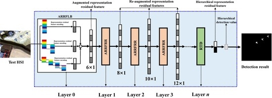
A Level-wise band-partition-based hierarchical representation residual feature (LBHRF) learning method for HTD is devised in a stepwise training manner without the need for back-propagation optimization. The SoftMax transformation, pooling operation, and augmented representation residual feature reuse and relearning among different layers are incorporated with cycle accumulation to enhance the nonlinear and discriminate feature learning capability of the method;
(2)
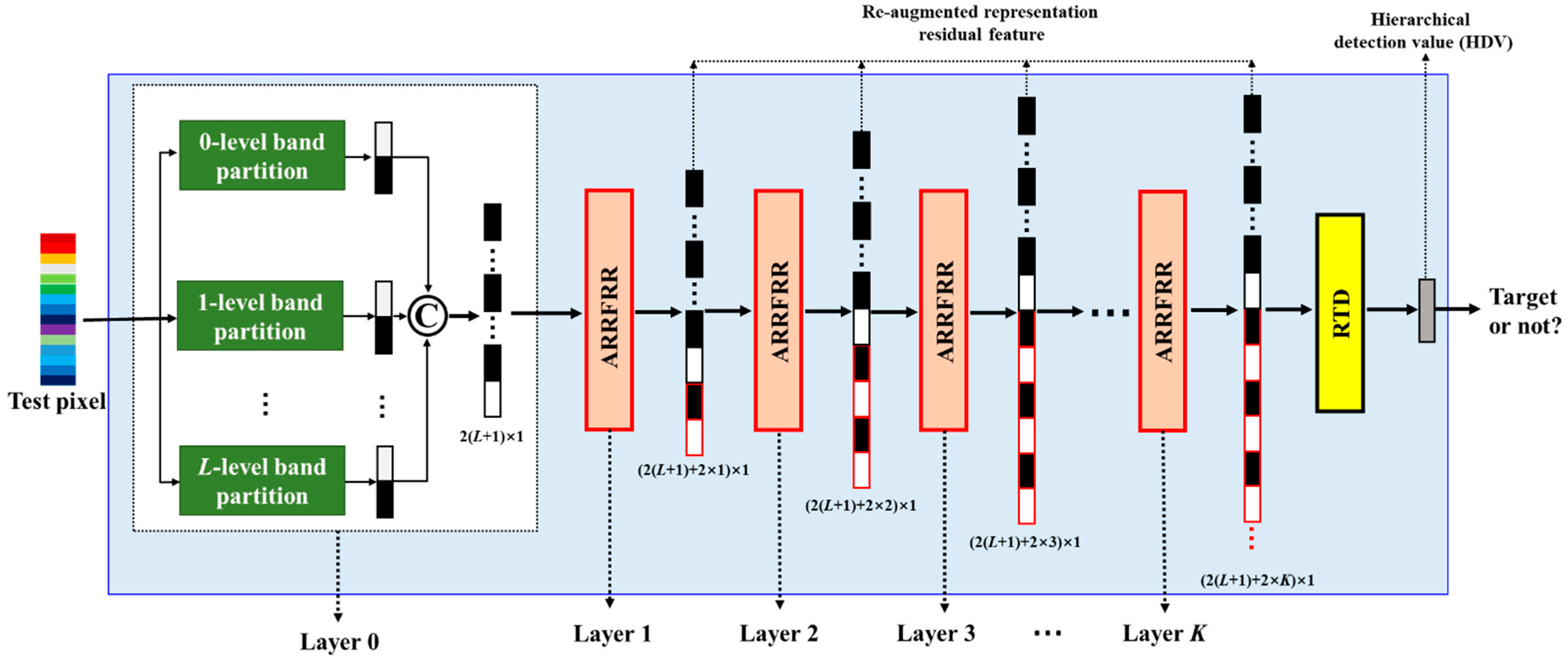
To flexibly integrate the global spectral integrity as well as the local contextual information of adjacent sub-bands, the original full spectral bands are partitioned into different levels with bands overlapping, and the augmented representation residual feature is then obtained by concatenating different levels of representation residual features;
(3)
Due to computational efficiency, the collaborative representation with the minimization of the l2-norm regularized representation coefficient is used in the experiments, and the results on several HSI target detection tasks show that the proposed method can yield overall superior detection performance.
The rest of this paper is structured as follows. Section 2 describes related work on HTD. Our LBHRF model for HTD is presented in Section 3, including the key modules ARRFLB, ARRFRR, and RTD. The effectiveness of the proposed method is demonstrated by experimental results presented in Section 4. Conclusions are made in Section 5.

2. Related Work

Consider a hyperspectral image having N pixels with B spectral bands, and all the spectra of an HSI are arranged in a B × N matrix as X = [ x i ,   x 2 , ,   x N ] R B × N containing the targets of interest for detection. The combined dictionary with known target and background pixels is denoted as A = [ A t , A b ] , where A t indicates the prior target spectra, and A b is the estimated background spectra. The purpose of HTD is to distinguish a label-unknown test pixel y R B as a target pixel or not, with the help of target and background dictionary A . With the idea of linear spectral mixing, it is assumed that the test pixel y can be represented as a linear combination of the pixels in the target and background dictionary A with representation coefficient vector α = [ α t , α b ] as follows.
y = A t α t + A b α b
The prestigious sparse representation-based target detector (SRD) seeks a spare representation coefficient vector α , which means the test pixel y is approximately represented by very few pixels from the combined dictionary A , and the recovered representation residuals can be used for detection. The mathematical formulation for SRD is expressed as follows,
α * = a r g m i n   α 0 s . t . y = A α
where · 0 means the l0-norm defined as the number of nonzero entries of a vector. The nonzero entries of α can help reveal the category of a test pixel y . The l0-norm minimizing problem (2) is NP-hard, and can be approximately solved by some greedy pursuit algorithms such as orthogonal matching pursuit (OMP) or subspace pursuit (SP) [22]. If the solution is sufficiently sparse, the NP-hard problem can be relaxed into a linear programming one by replacing the l0-norm with l1-norm, which can be solved by convex programming techniques. Considering the existence of noise in data, the equality constraint in (2) is relaxed to the following inequality one.
argmin α   α 0 s . t . A α y 2 θ
where θ is the upper bound for representation error. The above problem can also be formulated as the minimization of the representation error under a certain sparsity level.
argmin α   A α y 2 s . t . α 0 K 0
where K 0 is a given upper bound on the sparsity level. After solving (3) or (4), the optimal representation α = [ α t , α b ] will be obtained. Then, the background pixels A b and target pixels A t in dictionary A are used to reconstruct the test pixel by combining their corresponding sub-coefficients α t and α b , by which the representation residuals can be obtained as follows:
r b x = y A b α b 2
r t x = y A t α t 2
The smaller the representation residuals under each category of sub-dictionary, the more likely that the test pixel belongs to this category. Therefore, the difference between these two residuals under the two sub-dictionaries is used to calculate the detection value.
D S R D y = r b y r t y
Whether the pixel belongs to the background class or target class is determined according to the relationship between the detection value with specific threshold value. If the detection value D S R D y is greater than specific threshold value, the test pixel will be claimed as target, otherwise it is more likely to be background. The core idea behind the optimization problem (4) is that the test pixel will be represented by limited pixels similar to it under the constraint of representation error tolerance and sparsity. However, it is argued that it is the collaborative representation mechanism, but not the sparsity, that plays the essential role, as formulated below.
argmin α   α 2 s . t . A α y 2 δ
In addition, the l2-norm regularized collaborative representation mechanism has significantly lower computational complexity. Many variants of SRD based on collaborative representation mechanism have been studied, such as SDRD [22] and sparse representation-with binary hypothesis detector (SRBBH) [23].
It is not difficult to draw the conclusion that the above HTD methods can be summarized as class-specific representation residuals learning and comparison, by using different representation learning strategies. The derived representation residuals contain valuable discriminate information for HTD. However, these methods all perform one-round of representation learning and representation residuals calculation on the original full spectral bands. As a result, it is unable to make full use of the identification ability of different spectral bands for different materials, and the discriminant information implied in the representation residual cannot be sufficiently explored.

3. Level-Wise Band-Partition-Based Hierarchical Representation Residual Feature Learning for HTD

3.1. Parallel Level-Wise Band-Partition

In practice, HSI is obtained by a spectrometer in response to the electromagnetic wave reflected or emitted from the ground object material surface. Different materials have their unique responses to the electromagnetic wave. As a result, using the same full spectral bands to detect targets of different materials cannot make full use of discriminate information of different spectral bands and inevitably suffer from spectral redundancy. To alleviate the problem, this paper proposes to jointly use sub-band combinations based on level-wise band-partition together with the original full bands. For the l-th (l = 0, 1, 2, …, L) level, a total of 2 l sub-band combinations will be obtained. For example, the 2-th level of band-partition will have 2 2 = 4 sub-band combinations. Level 0 band-partition is the original full spectral bands themselves. For a test pixel y , the 1-th level band-partitions are denoted as y 1 = y 1 1 , y 2 1 , and similarly the l-th band partitions are illustrated as y l = y 1 l , y 2 l , , y 2 l l . y j i means the j-the sub-band combination of y in i-th level. As for the target and background dictionary, A j i collects the j-the sub-band combinations of A in the i-th level. Accordingly, the level l band-partition for the k-th sample of A is denoted as a k l = [ a 1 k l , a 2 k l , , a 2 l k l ] . Figure 2 shows an example process of Level 1 double-partition of a HSI pixel. For this level of band partition, all the pixels are partitioned into two parts with several bands overlapping, and all the pixels are partitioned in the same way to construct the band-partitioned target and background dictionaries.

3.2. Augmented Representation Residual Feature Based on Level-Wise Band-Partition (ARRFLB)

All the pixels in the target and background dictionary A and the test pixel y are first band-partitioned in the same way. Afterwards, for the j-th band-partition combinations of the i-th level, the corresponding band-partitioned test pixel y j i is represented using A j i by solving the following problem.
β * = argmin β A j i β y j i 2 2 + λ 1 β p
where · p is the p-norm used to regularize the representation coefficient β , and p = 0, 1, or 2 is usually adopted for l0, l1, or l2-norm minimization. λ 1 > 0 is used to balance two terms in the objective function. After solving (9), the target and background sub-dictionaries A b · j i and A t · j i are used to calculate the representation residuals of y j i as below.
r b · j i = y j i A b · j i β b 2
r t · j i = y j i A t · j i β t 2
Afterwards, the above two representation residual values are concatenated as a 2-dimensional representation residual feature, and used to encode the test pixel y j i in the j-th band-partition of the i-th level as in (12).
y j i = [ r b · j i ; r t · j i ]
To strengthen the discrimination of representation residual feature, the SoftMax operation is used to recompute a 2-dimensional representation residual feature as follows:
y j i = [ e r b · j i e r b · j i + e r t · j i ; e r t · j i e r b · j i + e r t · j i ]
For the l-th level band-partition, 2l representation residual feature with SoftMax, i.e., y j l   j = 1 , 2 , , 2 l , will be obtained, which is then transformed into one representation residual feature using the max pooling operation.
y l = m a x y 1 l ; y 2 l ; ; y 2 l l
Alternatively, the average pooling operation can be adopted to fuse the information from the 2 l band-partitions in l-th level.
y l = a v e r a g e y 1 l ; y 2 l ; ; y 2 l l
Afterwards, all the representation residual features processed by the SoftMax, and pooling operations from all the L levels of band-partitions are augmented and concatenated together to obtain a 2(L + 1)-dimensional augmented representation residual feature as follows.
y = y 0 ; y 1 ; ; y L R 2 L + 1 × 1
In addition to encoding the test pixel y and get its augmented representation residual feature y based on band-partitioned target and background dictionary as above, all the pixels of target and background dictionary are also encoded on the target and background dictionary itself to get their corresponding augmented representation residual features. Figure 3 shows an example for encoding augmented representation residual feature based on three levels of band-partition, all the pixels are encoded as a 6-dimensional representation residual feature using three levels (L = 2) of target and background dictionary. Therefore, the subtle discriminate information from different sub-band combinations and representation residuals is fused by the 6-dimensionl augmented representation residual feature.

3.3. Augmented Representation Residual Feature Reuse and Relearning (ARRFRR)

After parallel L levels of band-partition, all the pixels in the target and background dictionary A and the test pixel y are represented as a 2(L + 1)-dimensional augmented representation residual feature, which are formulated as A R 2 L + 1 × N and y R 2 L + 1 × 1 , respectively. It is known that the test pixel can be categorized as the class with minimum representation residual in a sparse representation-based target detector. In other words, the representation residuals contain significant discrimination information to distinguish targets from the background. However, the subtle discriminant information in representation residual might not be sufficiently exploited via such a one-round shallow learning strategy. In the following section, an augmented representation residual feature reuse and relearning (ARRFRR) method will be developed to serve as a key module for learning re-augmented representation residual feature.
In Layer 1, the input augmented representation residual feature is acquired as A 0 = A and y 0 = y . The representation coefficient learning of y 0 on A 0 is formulated as follows:
m i n   A 0 ϕ 0 y 0 2 2 + λ 2 ϕ 0 p
where   · p is the p-norm used to regularize the corresponding representation, and p can be 0, 1, or 2 for l0, l1, or l2-norm minimization. Different value of p will lead to different optimization problem. For example, when p = 2, a closed-form solution can be achieved, as follows.
ϕ 0 = A 0 1 A 0 + λ 2 I 1 y 0 1 y 0
After solving (16), the target and background sub-dictionaries A t 0 and A b 0 are used to calculate the representation residuals of y 0 as below.
R t 0 = A t 0 ϕ t 0 y 0 2
R b 0 = A b 0 ϕ b 0 y 0 2
The corresponding representation residual feature with SoftMax is calculated as follows:
s y 0 1 = [ e R b 0 e R b 0 + e R t 0 ; e R t 0 e R b 0 + e R t 0 ]
Then the original augmented representation feature and the above SoftMax vector are concatenated to obtain the re-augmented representation residual feature in Layer 1 as follows:
y 1 = [ y 0 ; s y 0 1 ]
According to the procedures presented in Equations (17)–(21), all the augmented representation residual features in A are re-augmented and updated. As shown in Figure 4, with level-wise band-partition, all the pixels are processed to obtain the corresponding re-augmented representation residual features, and construct the re-augmented representation residual feature dictionary. Afterwards, as shown in ①, each augmented representation residual feature is further represented using the representation residual feature dictionary to relearn the representation residual feature. The relearned representation residual feature is recomputed with SoftMax and concatenated with the original augmented representation residual feature by identity map, as shown in ②. Finally, the re-augmented representation residual feature is used to update the re-augmented representation residual feature dictionary as in ③.
The procedures shown in Figure 4 execute in cycle for K layers to derive the final K-th layer re-augmented representation residual feature dictionary A K = A 0 ; s A 1 ; ; s A K R 2 L + 1 + 2 K × N and y K = y 0 ;   s y 0 , ,   s y K R 2 L + 1 + 2 K × N , with L = 0 , 1 , 2 as the levels of band-partition and K = 0 , 1 , 2 as the layers for augmented representation residual feature reuse and relearning, which are further fed into the representation-based target detector (RTD) as follows.
min ϕ K A K ϕ K y K 2 2 + λ 2 ϕ K p
With the optimal representation coefficient ϕ K in K-th layer, the final hierarchical detection value (HDV) in the output of the K-th layer is calculated as shown below.
H D V K = A b K ϕ b K y K 2 A t K ϕ t K y K 2
If the detection value is bigger than a predefined threshold, the original test pixel y will be labeled as a target pixel; otherwise, the test pixel is a background pixel. The details for hyperspectral target detection using LBHRF are summarized in Algorithm 1.
Algorithm 1: The proposed LBHRF learning method for hyperspectral target detection.
Input: Test pixel y . Target prior spectra and background dictionaries A . The band-partition level L. The layer K.
1: Learn the L levels augmented representation residual feature for all the target and background pixels A and test pixel y via ARRFLB presented in Equations (8)–(14);
2: Initialize k = 1;
3: Repeat;
4: Learn the k-th layer re-augmented representation residual features A k and y k  for the target and background dictionary pixels and the test pixel based on the augmented representation residual feature A and y by ARRFRR presented in Equations (17)–(22);
5: k = k + 1;
6: Until k > K;
7: Calculate the hierarchical detection value by RTD as presented in Equations (23) and (24).
Output: The hierarchical detection value H D V K for target detection.

4. Experimental Results and Analysis

4.1. Hyperspectral Data Set

The first data set was collected by the HYDICE sensor [21] with a spatial resolution of 2 m and 210 spectral bands. After removing the low SNR, water absorption and bad bands (1–4, 76, 87, 101–111, 136–153, and 198–210), 162 bands remained. The HYDICE data set and its ground-truth information are shown in Figure 5, which has 150 × 150 pixels, and the vehicles were selected as the targets to detect, which have 21 pixels.
The second and third data sets are collected by the AVIRIS from San Diego with a spatial resolution of 3.5 m. After removing the low SNR, water absorption, and bad bands (1–6, 33–35, 97, 107–113, 153–166, and 221–224), 189 bands were remained. The AVIRIS I data set and AVIRIS II data set and their ground-truth information are shown in Figure 6 and Figure 7, which are 60 × 60 pixels and 100 × 100 pixels in size, respectively.
The proposed LBHRF HTD method is evaluated in comparison to the several advanced HSI target detectors, including constrained energy minimization (CEM) [15], sparse representation-based target detector (SRD) [20], sparse representation-with binary hypothesis detector (SRBBH) [23], binary-class collaborative representation-based detector (BCRD) [21], sparse and dense hybrid representation-based detector (SDRD) [22], and single-spectrum-driven binary-class sparse representation target detector (SSBRTD) [29]. In summary, the comparing methods include classic target methods, i.e., CEM and the state-of-the-art representation learning based methods, i.e., SRD, SRBBH, BCRD, SDRD, and SSBRTD. For a fair comparison between different detectors, the widely used dual concentric window strategy is adopted to estimate the background characteristic around each test pixel. For our LBHRF HTD method, the l2-norm is used to regularize the representation coefficient in the two basic residual feature learning modules, i.e., p = 2 in Equations (9) and (10).
To evaluate the performance of different detection methods, the probability of false alarm (PF), and probability of detection (PD) under different threshold variables τ are calculated [30]. In addition, the ROC curves w.r.t. (PF, PD) and (τ, PF) are used to reveal the target detectability and background suppression of each detection method. The area under curve (AUC) corresponding to the two ROC curves are used to quantitatively evaluate the performance of different detection methods. A detection method with a higher A U C ( P F , P D ) approaching 1 (→1) and a lower A U C ( τ , P F ) close to 0 (→0) is judged to have better performance for target detection as well as background suppression [30]. Without good background suppression ability, a HSI detector cannot guarantee a sufficiently low false alarm rate. Additionally, the ratio between the two AUC values, i.e., A U C ( r a t i o ) = A U C ( P F , P D ) / A U C ( τ , P F ) , can be calculated to comprehensively consider the balance ability of a detector in both target detectability and background suppression [30].

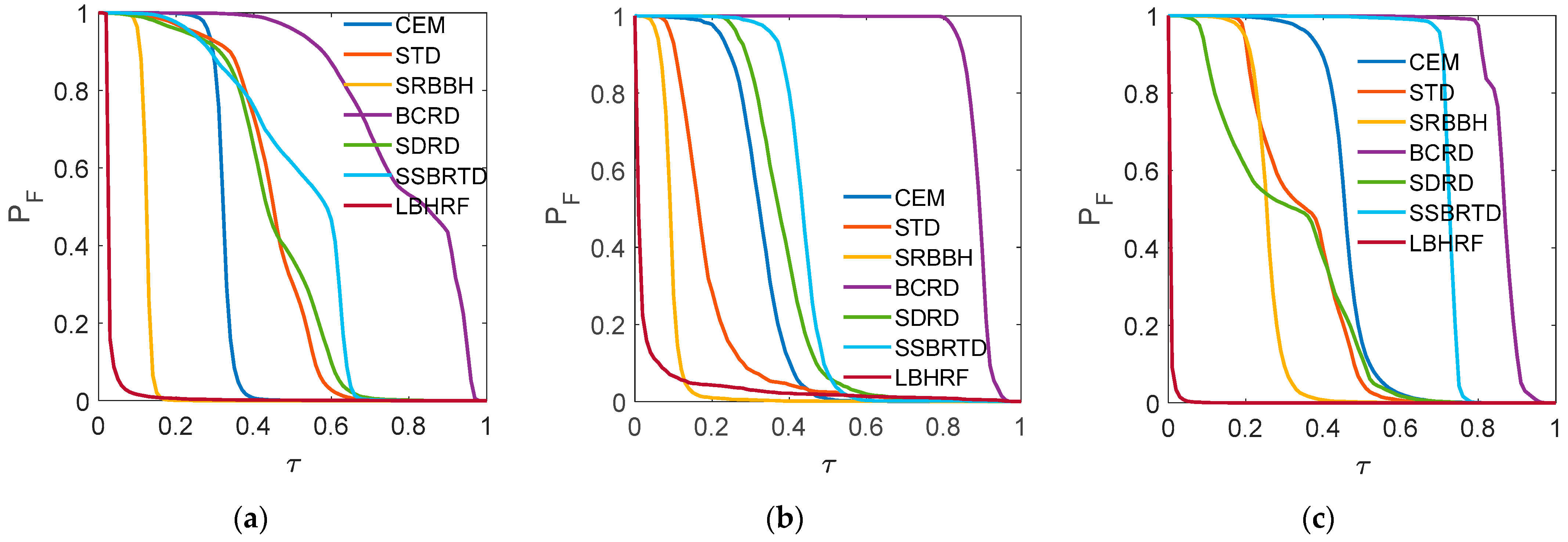
4.2. Experimental Results

First, the qualitative detection results of different detection methods are demonstrated. The 2D visualization detection results of different HSI target detectors on the three data sets are shown in Table 1. From the qualitative visualization results, one can observe that LBHRF method can generate a more conspicuous target distribution when comparing with the ground-truth and detection results of the comparing counterparts. In detail, the targets detected by the proposed LBHRF method have a clearer shape with a purer background, which means a better ability for both target detection and non-target background suppression. By contrast, the detection results of the comparing methods cannot clearly distinguish the targets, and the background component has strong interference in the detection results.
It is generally known that for a HTD task, a high-performance detector should have significantly strong responses for the target pixels and simultaneously possesses strong inhibition ability for non-target background pixels, which can lead to a higher probability of detection rate by preserving lower false alarm rate. For a quantitative evaluation, the ROC curves w.r.t. (PF, PD) and (τ, PF) are drawn and shown in Figure 8 and Figure 9 to further demonstrate the target detectability and background inhibition characteristics of different detectors. In addition, the AUC values, i.e., AUC(PF, PD) and AUC(τ, PF) that correspond to the two kinds of ROC curves are reported in Table 2 and Table 3, where the best results are indicated in bold and the second-best results are underlined.
As Figure 8 shows, the ROC curve of the proposed LBHRF method w.r.t. (PF, PD) is closer to the upper left part of each figure when comparing with the other methods. The corresponding quantitative AUC(PF, PD) value given in Table 2 also validates this point, and the proposed method can generally achieve a higher AUC(PF, PD) value, which means a better overall detection performance. Moreover, the ROC curves of the proposed LBHRF method w.r.t. (τ, PF) shown in Figure 9 approach nearer to the lower left part of each figure than that of the other methods. Similarly, the AUC(τ, PF) values listed in Figure 9 correspond to Figure 9 also indicate that the proposed LBHRF can yield lower AUC(τ, PF) values. When comprehensively considering the balance between AUC(PF, PD) and AUC(τ, PF), i.e., the AUC(ratio) reported in Table 4, our LBHRF method presents an incomparable obvious advantage over the other methods. In general, the benefits of the LBHRF method can be attributed to the multi-level and multi-layer residual feature learning and augmentation, and the discriminate information is accumulated in the obtained augmented representation residual feature for improved overall detection performance.

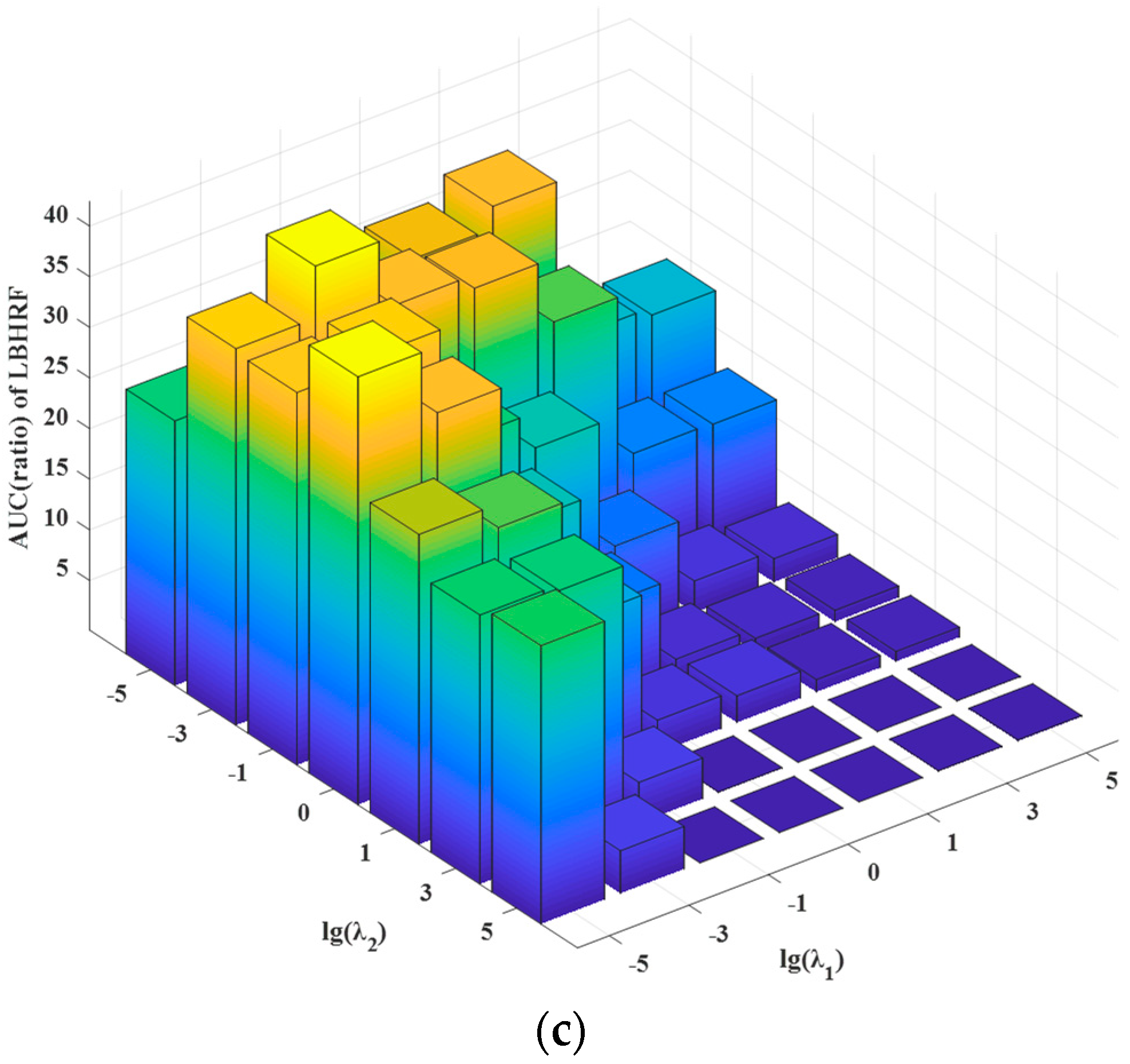
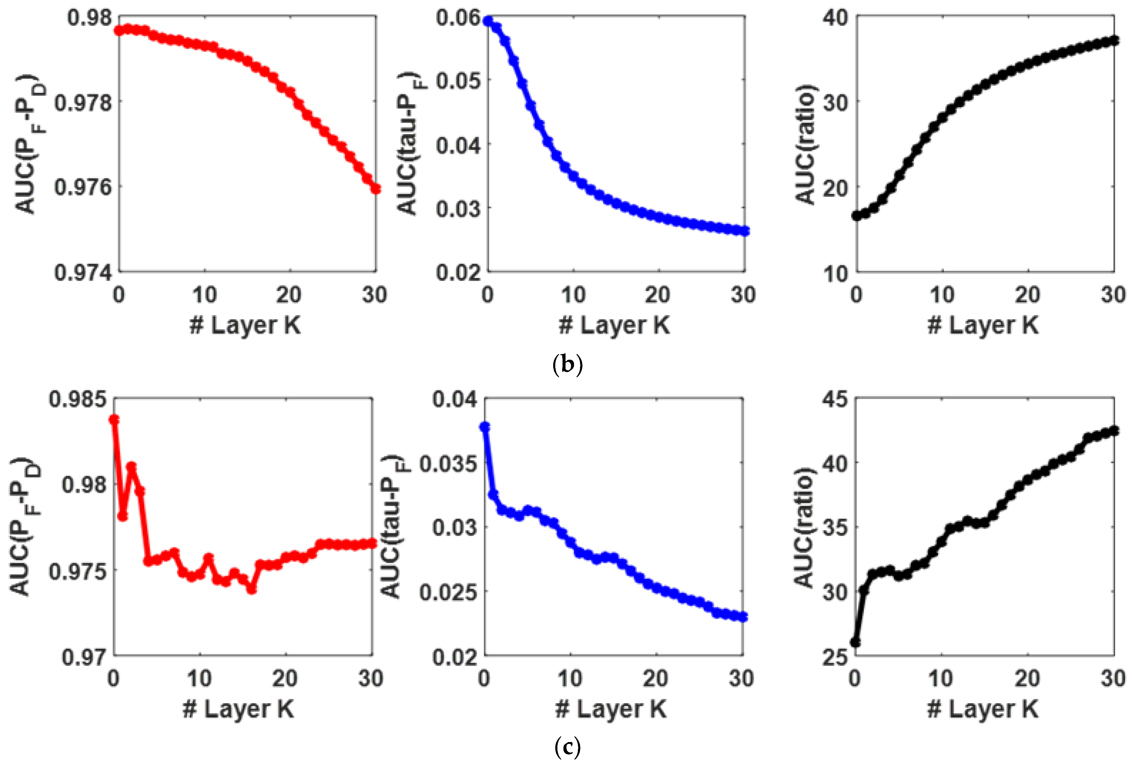
4.3. Parameters Sensitivity Analysis

In Section 3.2, the augmented representation residual feature learning based on level-wise band-partition is presented, and there is an adjustable trade-off parameter λ 1 in Equation (9). In the experiments, λ 1 is set and remain unchanged for all the different band-partition combinations under different levels. In addition to λ 1 , trade-off parameter λ 2 in Equations (17) and (22) also needs to be set for augmented representation residual feature reuse and relearning. For simplicity, λ 2 is also assigned and remains unchanged for different layers of residual feature learning. As a result, this section will study the influences of λ 1 and λ 2 on the final detection performance. Specifically, the AVIRIS I HSI data set is used as an example, and λ 1 and λ 2 are both selected from the parameter candidate set 10 5 , 10 3 , 10 1 , 1 , 10 , 10 3 , 10 5 when L = 0, 1, 2 with varying K.
In Section 3.3, the final re-augmented representation residual feature for target and background dictionary and test pixel, i.e., the resulting A K R 2 L + 1 + 2 K × N and y K R 2 L + 1 + 2 K × N are fed into the RTD for HDV calculation and target detection as in Equations (22) and (23). Therein, L means the levels of band-partition and K indicates the layers for augmented representation residual feature reuse and relearning. The target detectability and background suppressible in terms of the ROC curves w.r.t. (PF, PD) and (τ, PF) of our LBHRF detector are studied under different settings of L and K. To be specific, L = 0, 1, 2 is considered when K varies from 0 to the deepest layer of 30. It is worth noting that L = 0 means that only the original full spectral bands are utilized without band-partition for LBHRF detector construction. Also, K = 0 means that the augmented representation residual feature with 2 L + 1 dimensions obtained from the L levels of band-partition is directly fed into the ultimate RTD for category judgement of a test pixel.
Figure 10 shows the AUC(ratio) performance variation of the proposed LBHRF method in terms of varying λ 1 and λ 2 when band-partition level L = 0, 1, 2. For each individual figure, when λ 1 and λ 2 fall in the scopes of [ 10 5 , 1 ] and [ 10 5 , 10 3 ] , respectively, the proposed LBHRF method tends to achieve a better and more stable AUC(ratio) performance. In addition, when L increases from 0 to 2, our LBHRF method can gradually yield better AUC(ratio) performance, which shows the band-partition strategy used for the residual feature learning and augmentation helps to improve the target detection and background suppression performance.
In addition, the changes for the A U C ( P F , P D ) , A U C ( τ , P F ) , and AUC(ratio) performance of the proposed LBHRF method when L = 0 and K varies from 0 to 30 are displayed in Figure 11. From the figures, it is not difficult to conclude that A U C ( P F , P D ) , A U C ( τ , P F ) , and AUC(ratio) values of the proposed LBHRF method show a similar change trend with varying band-partition level L. Specifically, the overall performance indicator A U C ( P F , P D ) is inclined to decrease when K increases from 0 to 30, and at the same time the A U C ( τ , P F ) values also tend to decrease. In addition, it is noteworthy that the decreasing ratios of A U C ( τ , P F ) values are larger than that of A U C ( P F , P D ) values. For example, when L = 0, the A U C ( P F , P D ) value decreases from about 0.975 to around 0.96 with a decreasing ratio of 1.53%. Meanwhile, the A U C ( τ , P F ) value decreases from about 0.06 to around 0.03, and the decreasing ratio reaches about 50%. The results demonstrate that when the residual feature learning and augmentation layer goes deeper, the overall target detectability decrease slightly and the background inhibition ability improves significantly, which can lead to a better overall AUC(ratio) performance, as demonstrated in Figure 11. In practice, a smaller layer K can be set when a higher overall target detectability is preferred. When a stronger background suppression ability is desired, a larger layer K will be preferred for parameter setting.

4.4. Discussion

When designing a target detector for HSI, there are two key characteristics that should be generally considered, i.e., the target detection ability as well as the background suppression capacity. A fine target detector should ensure a high true positive rate as well as a strong background suppression ability, which can reduce the false positive rate. The experimental results show that the existing representation learning-based HTD methods with original full spectral bands underperform comparatively on the three HSI target detection tasks. The reason of which is that the one-round residual feature learning strategy cannot make full use of the rich spectral information to detect target from background.
By comparison, the proposed LBHRF method aims to sufficiently utilize the global full spectra as well as the contextual information of adjacent local sub-band combinations. In addition, the SoftMax transformation, pooling operation, and representation residual feature reuse and re-augmentation are equipped in cascade to enhance the nonlinear learning ability of the LBHRF method. With the learning methodology, our LBHRF method can progressively discover and converge the underlying discriminant information in both global full bands and the local sub-bands combinations, and the finally obtained augmented representation residual feature with RTD can well distinguish the highly-mixed target and background pixels by highlighting target and inhibiting background, which are verified by the above qualitative and quantitative analysis.

5. Conclusions

This paper revisits the prestigious representation learning-based HTD methods, and finds that the detection performance of which will be restricted by the one-round shallow residual feature learning on the original full spectral bands. To alleviate the problem, this paper proposes to divide and congregate different levels of sub-band spectral bands combinations for multi-level and multi-layer residual feature learning and augmentation, and thus the discriminate information that are beneficial for distinguishing targets from background can be accumulated in the obtained augmented residual feature. Experimental results on different HSI target detection tasks show that the proposed LBHRF method can not only achieve an leading overall target detection performance, i.e., a higher AUC(PF, PD) value, but also obtain a significant improvement in background suppression ability, i.e., a lower AUC(τ, PF) value, in comparison to some representative state-of-the-art representation learning-based HTD methods. Future work will consider introducing spatial information into our method for further improvement. In addition, the construction of a more efficient universal background dictionary will be studied in future.

Author Contributions

All the authors made significant contributions to the study. T.G. and F.L. conceived and designed the global structure and methodology of the manuscript. T.G. and F.L. wrote and proofread the manuscript. Y.D., X.H. and G.S. provided some valuable advice and proofread the manuscript. All authors have read and agreed to the published version of the manuscript.

Funding

This work was supported in part by the National Natural Science Foundation of China under Grant 62201109, 62071340 and 42201371, in part by the Natural Science Foundation of Chongqing under Grant CSTB2022NSCQMSX0452, in part by the Key Scientific and Technological Innovation Project for “Chengdu-Chongqing Double City Economic Circle” under grant KJCXZD2020025, in part by the Macao Young Scholars Program under Grant AM2020008, and in part by the Fundamental Research Funds for the Central Universities under Grant 2023CDJXY-039.

Data Availability Statement

Data will be available on request.

Conflicts of Interest

The authors declare no conflict of interest.

References

  1. Gao, L.; Han, Z.; Hong, B.; Zhang, B.; Chanussot, J. CyCU-Net: Cycle-consistency unmixing network by learning cascaded autoencoders. IEEE Trans. Geosci. Remote Sens. 2022, 60, 5503914. [Google Scholar] [CrossRef]
  2. Guo, T.; Wang, R.; Luo, F.; Gong, X.; Zhang, L.; Gao, X. Dual-View Spectral and Global Spatial Feature Fusion Network for Hyperspectral Image Classification. IEEE Trans. Geosci. Remote Sens. 2023, 61, 5512913. [Google Scholar] [CrossRef]
  3. Luo, F.; Zou, Z.; Liu, J.; Lin, Z. Dimensionality reduction and classification of hyperspectral image via multi-structure unified discriminative embedding. IEEE Trans. Geosci. Remote Sens. 2022, 60, 5517916. [Google Scholar] [CrossRef]
  4. Luo, F.; Zhou, T.; Liu, J.; Guo, T.; Gong, X.; Ren, J. Multi-Scale Diff-changed Feature Fusion Network for Hyperspectral Image Change Detection. IEEE Trans. Geosci. Remote Sens. 2023, 61, 5502713. [Google Scholar] [CrossRef]
  5. Duan, Y.; Luo, F.; Fu, M.; Niu, Y.; Gong, X. Classification via Structure Preserved Hypergraph Convolution Network for Hyperspectral Image. IEEE Trans. Geosci. Remote Sens. 2023, 61, 5507113. [Google Scholar] [CrossRef]
  6. Guo, T.; Luo, F.; Zhang, L.; Zhang, B.; Tan, X.; Zhou, X. Learning Structurally Incoherent Background and Target Dictionaries for Hyperspectral Target Detection. IEEE J. Sel. Top. Appl. Earth Obs. Remote Sens. 2020, 13, 3521–3533. [Google Scholar] [CrossRef]
  7. Zeng, J.; Wang, Q. Sparse Tensor Model-Based Spectral Angle Detector for Hyperspectral Target Detection. IEEE Trans. Geosci. Remote Sens. 2022, 60, 5539315. [Google Scholar] [CrossRef]
  8. Guo, T.; He, L.; Luo, F.; Gong, X.; Li, Y.; Zhang, L. Anomaly Detection of Hyperspectral Image with Hierarchical Anti-Noise Mutual-Incoherence-Induced Low-Rank Representation. IEEE Trans. Geosci. Remote Sens. 2023, 61, 5510213. [Google Scholar] [CrossRef]
  9. Zhou, H.; Luo, F.; Zhuang, H.; Weng, Z.; Gong, X.; Lin, Z. Attention Multi-Hop Graph and Multi-Scale Convolutional Fusion Network for Hyperspectral Image Classification. IEEE Trans. Geosci. Remote Sens. 2023, 61, 5508614. [Google Scholar] [CrossRef]
  10. Luo, F.; Huang, H.; Ma, Z.; Liu, J. Semi-supervised sparse manifold discriminative analysis for feature extraction of hyperspectral images. IEEE Trans. Geosci. Remote Sens. 2016, 54, 6197–6221. [Google Scholar] [CrossRef]
  11. Guo, T.; Luo, F.; Fang, L.; Zhang, B. Meta-Pixel-Driven Embeddable Discriminative Target and Background Dictionary Pair Learning for Hyperspectral Target Detection. Remote Sens. 2022, 14, 481. [Google Scholar] [CrossRef]
  12. Gao, L.; Wang, D.; Zhuang, L.; Sun, X.; Huang, M.; Plaza, A. BS3LNet: A new blind-spot self-supervised learning network for hyperspectral anomaly detection. IEEE Trans. Geosci. Remote Sens. 2023, 61, 5504218. [Google Scholar] [CrossRef]
  13. Theiler, J.; Ziemann, A.; Matteoli, S.; Diani, M. Spectral Variability of Remotely Sensed Target Materials: Causes, Models, and Strategies for Mitigation and Robust Exploitation. IEEE Geosci. Remote Sens. Mag. 2019, 7, 8–30. [Google Scholar] [CrossRef]
  14. Liu, L.; Zou, Z.; Shi, Z. Hyperspectral Remote Sensing Image Synthesis Based on Implicit Neural Spectral Mixing Models. IEEE Trans. Geosci. Remote Sens. 2023, 61, 5500514. [Google Scholar] [CrossRef]
  15. Du, Q.; Ren, H.; Chang, C.-I. A comparative study for orthogonal subspace projection and constrained energy minimization. IEEE Trans. Geosci. Remote Sens. 2003, 41, 1525–1529. [Google Scholar]
  16. Guo, T.; Lu, X.-P.; Yu, K.; Zhang, Y.-X.; Wei, W. Integration of Light Curve Brightness Information and Layered Discriminative Constrained Energy Minimization for Automatic Binary Asteroid Detection. IEEE Trans. Aerosp. Electron. Syst. 2022, 58, 4984–4999. [Google Scholar] [CrossRef]
  17. Vincent, F.; Besson, O. One-Step Generalized Likelihood Ratio Test for Subpixel Target Detection in Hyperspectral Imaging. IEEE Trans. Geosci. Remote Sens. 2020, 8, 4479–4489. [Google Scholar] [CrossRef] [Green Version]
  18. Yang, S.; Shi, Z. SparseCEM and SparseACE for Hyperspectral Image Target Detection. IEEE Geosci. Remote Sens. Lett. 2014, 11, 2135–2139. [Google Scholar] [CrossRef]
  19. Liu, J.; Li, H.; Himed, B. Threshold Setting for Adaptive Matched Filter and Adaptive Coherence Estimator. IEEE Signal Process. Lett. 2015, 22, 11–15. [Google Scholar] [CrossRef]
  20. Chen, Y.; Nasrabadi, N.M.; Tran, T.D. Sparse Representation for Target Detection in Hyperspectral Imagery. IEEE J. Sel. Top. Signal Process. 2011, 5, 629–640. [Google Scholar] [CrossRef]
  21. Zhu, D.; Du, B.; Zhang, L. Binary-Class Collaborative Representation for Target Detection in Hyperspectral Images. IEEE Geosci. Remote Sens. Lett. 2019, 16, 1100–1104. [Google Scholar] [CrossRef]
  22. Guo, T.; Luo, F.; Zhang, L.; Tan, X.; Liu, J.; Zhou, X. Target Detection in Hyperspectral Imagery via Sparse and Dense Hybrid Representation. IEEE Geosci. Remote Sens. Lett. 2020, 17, 716–720. [Google Scholar] [CrossRef]
  23. Zhang, Y.; Du, B.; Zhang, L. A Sparse Representation-Based Binary Hypothesis Model for Target Detection in Hyperspectral Images. IEEE Trans. Geosci. Remote Sens. 2014, 53, 1346–1354. [Google Scholar] [CrossRef]
  24. Zhu, D.; Du, B.; Zhang, L. Target Dictionary Construction-Based Sparse Representation Hyperspectral Target Detection Methods. IEEE J. Sel. Top. Appl. Earth Obs. Remote Sens. 2019, 12, 1254–1264. [Google Scholar] [CrossRef]
  25. Wright, J.; Yang, A.Y.; Ganesh, A.; Sastry, S.S.; Ma, Y. Robust Face Recognition via Sparse Representation. IEEE Trans. Pattern Anal. Mach. Intell. 2009, 31, 210–227. [Google Scholar] [CrossRef] [Green Version]
  26. Zhang, L.; Liu, J.; Zhang, B.; Zhang, D.; Zhu, C. Deep Cascade Model Based Face Recognition: When Deep-Layered Learning Meets Small Data. IEEE Trans. Image Process. 2020, 29, 1016–1029. [Google Scholar] [CrossRef]
  27. Tong, F.; Zhang, Y. Exploiting Spectral-Spatial Information Using Deep Random Forest for Hyperspectral Imagery Classification. IEEE Geosci. Remote Sens. Lett. 2022, 19, 5509505. [Google Scholar] [CrossRef]
  28. Tang, J.; Deng, C.; Huang, G.-B. Extreme Learning Machine for Multilayer Perceptron. IEEE Trans. Neural Netw. Learn. Syst. 2016, 27, 809–821. [Google Scholar] [CrossRef]
  29. Zhu, D.; Du, B.; Zhang, L. Single-spectrum-driven binary-class sparse representation target detector for hyperspectral imagery. IEEE Trans. Geosci. Remote Sens. 2021, 59, 1487–1500. [Google Scholar] [CrossRef]
  30. Chang, C.-I. Comprehensive analysis of receiver operating characteristic (ROC) curves for hyperspectral anomaly detection. IEEE Trans. Geosci. Remote Sens. 2022, 60, 5541124. [Google Scholar] [CrossRef]
Figure 1. Illustration for the structure of the proposed level-wise band-partition-based hierarchical representation residual feature (LBHRF) learning method with L levels of band-partition and K layers for HTD. Different color means different spectral band.
Remotesensing 15 03608 g001
Figure 2. The process of Level 1 double-partition of the original full spectral band. For this level of band partition, all the pixels are partitioned into two parts with several bands overlapping, and the Level 1 target and background dictionary are accordingly obtained in the same way. Different color means different spectral band.
Remotesensing 15 03608 g002
Figure 3. Illustration for the augmented representation residual feature based on level-wise band-partition (ARRFLB) with 0, 1, and 2 levels. Through the processing, each pixel is encoded as a 6-dimensionl augmented representation residual feature. If L (≥0) levels of band-partition are adopted, an augmented representation residual feature with 2(L + 1) dimensions will be obtained.
Remotesensing 15 03608 g003
Figure 4. Augmented representation residual feature reuse and relearning module to calculate the corresponding re-augmented representation residual feature.
Remotesensing 15 03608 g004
Figure 5. HYDICE image scene and the ground-truth.
Remotesensing 15 03608 g005
Figure 6. AVIRIS I image scene and the ground-truth.
Remotesensing 15 03608 g006
Figure 7. AVIRIS II image scene and the ground-truth.
Remotesensing 15 03608 g007
Figure 8. ROC performance of different HTD methods w.r.t. (PF, PD) on different data sets. (a) HYDICE; (b) AVIRIS I; (c) AVIRIS II.
Remotesensing 15 03608 g008
Figure 9. ROC performance of different HTD methods w.r.t. (τ, PF) on different data sets. (a) HYDICE; (b) AVIRIS I; (c) AVIRIS II.
Remotesensing 15 03608 g009
Figure 10. The AUC(ratio) performance of the proposed LBHRF in terms of varying λ 1 and λ 2 when L = 0, 1, 2, respectively. (a) L = 0; (b) L = 1; (c) L = 2.
Remotesensing 15 03608 g010aRemotesensing 15 03608 g010b
Figure 11. The A U C ( P F , P D ) , A U C ( τ , P F ) , and AUC(ratio) performance of the proposed LBHRF method when L = 0,1,2, when K varies from 0 to 30. (a) L = 0; (b) L = 1; (c) L = 2.
Remotesensing 15 03608 g011aRemotesensing 15 03608 g011b
Table 1. Visualization of detection results of different HTD methods on the three datasets.
Data SetsThe Comparing HSI Detectors
CEM [15]SRD [20]SRBBH [23]BCRD [21]SDRD [22]SSBRTD [29]LBHRFGround-Truth
HYDICERemotesensing 15 03608 i001Remotesensing 15 03608 i002Remotesensing 15 03608 i003Remotesensing 15 03608 i004Remotesensing 15 03608 i005Remotesensing 15 03608 i006Remotesensing 15 03608 i007Remotesensing 15 03608 i008
AVIRIS IRemotesensing 15 03608 i009Remotesensing 15 03608 i010Remotesensing 15 03608 i011Remotesensing 15 03608 i012Remotesensing 15 03608 i013Remotesensing 15 03608 i014Remotesensing 15 03608 i015Remotesensing 15 03608 i016
AVIRIS IIRemotesensing 15 03608 i017Remotesensing 15 03608 i018Remotesensing 15 03608 i019Remotesensing 15 03608 i020Remotesensing 15 03608 i021Remotesensing 15 03608 i022Remotesensing 15 03608 i023Remotesensing 15 03608 i024
Table 2. AUC(PF, PD)value comparison of different HTD methods on the three HSI datasets. The best result is in bold with the second-best result underlined.
MethodsData Sets
HYDICEAVIRIS IAVIRIS II
CEM [15]0.91390.65490.6983
SRD [20]0.98400.95610.9331
SRBBH [23]0.89090.89130.7224
BCRD [21]0.91750.98050.9899
SDRD [22]0.99730.95830.9921
SSBRTD [29]0.95970.90510.9689
LBHRF0.99780.98440.9987
Table 3. AUC(τ, PF) comparison of different HTD methods on the three HSI datasets. The best result is in bold with the second-best result underlined.
MethodsData Sets
HYDICEAVIRIS IAVIRIS II
CEM [15]0.32180.32360.4573
SRD [20]0.44590.18760.3421
SRBBH [23]0.12340.09360.2558
BCRD [21]0.79260.88880.8635
SDRD [22]0.44880.38120.3028
SSBRTD [29]0.51060.42870.7326
LBHRF0.03100.03880.0037
Table 4. AUC (ratio) comparison of different HTD methods on the three HSI datasets. The best result is in bold and the second-best result is in underline.
MethodsData Sets
HYDICEAVIRIS IAVIRIS II
CEM [15]2.84002.02381.5270
SRD [20]2.20685.09652.7276
SRBBH [23]7.21969.52242.8241
BCRD [21]1.15761.10321.1464
SDRD [22]2.22212.51393.2764
SSBRTD [29]1.87962.11131.3225
LBHRF32.187125.3711269.9189
Disclaimer/Publisher’s Note: The statements, opinions and data contained in all publications are solely those of the individual author(s) and contributor(s) and not of MDPI and/or the editor(s). MDPI and/or the editor(s) disclaim responsibility for any injury to people or property resulting from any ideas, methods, instructions or products referred to in the content.

