Article

Dual-Branch Fusion of Convolutional Neural Network and Graph Convolutional Network for PolSAR Image Classification

1
Department of Electrical and Computer Engineering, Memorial University of Newfoundland, St. John’s, NL A1B3X5, Canada
2
C-CORE, St. John’s, NL A1B 3X5, Canada
3
The Canada Centre for Mapping and Earth Observation, Ottawa, ON K1S 5K2, Canada
4
Department of Environmental Resources Engineering, State University of New York College of Environmental Science and Forestry (SUNY ESF), Syracuse, NY 13210, USA
*
Author to whom correspondence should be addressed.
Remote Sens. 2023, 15(1), 75; https://doi.org/10.3390/rs15010075
Submission received: 15 November 2022 / Revised: 16 December 2022 / Accepted: 20 December 2022 / Published: 23 December 2022

Abstract

:
Polarimetric synthetic aperture radar (PolSAR) images contain useful information, which can lead to extensive land cover interpretation and a variety of output products. In contrast to optical imagery, there are several challenges in extracting beneficial features from PolSAR data. Deep learning (DL) methods can provide solutions to address PolSAR feature extraction challenges. The convolutional neural networks (CNNs) and graph convolutional networks (GCNs) can drive PolSAR image characteristics by deploying kernel abilities in considering neighborhood (local) information and graphs in considering long-range similarities. A novel dual-branch fusion of CNN and mini-GCN is proposed in this study for PolSAR image classification. To fully utilize the PolSAR image capacity, different spatial-based and polarimetric-based features are incorporated into CNN and mini-GCN branches of the proposed model. The performance of the proposed method is verified by comparing the classification results to multiple state-of-the-art approaches on the airborne synthetic aperture radar (AIRSAR) dataset of Flevoland and San Francisco. The proposed approach showed 1.3% and 2.7% improvements in overall accuracy compared to conventional methods with these AIRSAR datasets. Meanwhile, it enhanced its one-branch version by 0.73% and 1.82%. Analyses over Flevoland data further indicated the effectiveness of the dual-branch model using varied training sampling ratios, leading to a promising overall accuracy of 99.9% with a 10% sampling ratio.

1. Introduction

Polarimetric synthetic aperture radar (PolSAR) has become of the utmost importance in land cover discrimination methods, providing extensive information about land features using fully polarized data, which are collected in almost all weather conditions, as well as day and night. This polarimetric information mainly considers features based on scattering mechanisms and overlooks spatial information, unlike other remote sensing images (e.g., optical and hyperspectral images). Therefore, accessing both polarimetric and spatial information from PolSAR images requires the extraction of additional features.
Several PolSAR feature extraction techniques have been developed and investigated for classification methods [1,2,3]. Due to the complexity of full polarimetric SAR images, features containing the most distinctive information are needed for different applications, including classification and change detection. Statistical features [4,5], scattering information [6], and target decomposition features [7,8,9] are the three main types of extracted features from PolSAR image analysis. Traditional PolSAR image analysis solves the classification problem in a two-step process, including feature extraction and classification. Accordingly, conventional PolSAR image classification methods, such as Wishart [10,11,12], decision tree [13,14], and support vector machine (SVM) [15,16], have been applied after the feature extraction step. The main disadvantage of these methods is that the feature engineering step is a time-consuming task and decreases the classification accuracy when high-correlated features or features with low information content are extracted in this step. In contrast to conventional PolSAR image classification algorithms, deep learning (DL) methods remove the feature engineering task from the processing steps. As such, the capability of different DL algorithms, such as a convolutional neural network (CNN) [17], autoencoder (AE) [18,19], and deep belief network (DBN) [20], were recently investigated for PolSAR image classification. Among these advanced models, deep CNNs have achieved remarkable success in PolSAR image classification [21,22]. As reported in the literature, utilizing a single convolutional kernel of CNN and single-channel CNN does not extract sufficient information for PolSAR image classification [23]. Therefore, several networks have been developed based on this algorithm with versatile structures and PolSAR features [24,25]. For example, Chen and Tao [25] derived several polarimetric features, including entropy (H), mean alpha angle, anisotropy from a decomposition technique, total backscattering power (SPAN), and two null angles for supervised image classification using the deep convolutional neural network (DCNN). Zhang, et al. [26] also proposed complex-valued CNN (CV-CNN) for PolSAR data processing by extending each element of real-valued CNN (RV-CNN), including feed-forward and backpropagation process, to the complex domain, wherein coherency matrix values were considered as complex inputs for the network. In order to benefit from rich spatial and polarimetric features of PolSAR data, multibranch CNNs have been proposed [27,28,29]. These networks contain independent CNNs for distinguishing different classes. In another study, Gao, et al. [27] developed a dual-branch CNN, which utilizes six-channel polarimetric and three-channel spatial features (Pauli RGB (red, green, blue)) as two independent inputs of the proposed model. Accordingly, a multichannel fusion of CNNs based on different scattering mechanisms was designated [28], in which each CNN obtains one of the Freeman decomposition elements (odd bounce, double-bounce, and volume scattering), and, together with a fusion feature, they passed through fully connected (FC) layers.
Graph-based DL methods have attracted great attention among remote sensing researchers for image classification. Graph convolutional networks (GCNs) [30] consider the relation between samples over the whole image rather than the local kernels of CNNs. In the case of PolSAR classification, there is a limited number of studies which have used GCNs. In contrast, GCNs have been widely utilized in hyperspectral image (HSI) classification [31,32,33,34]. For instance, He, et al. [35] presented supervised dual GCN (DGCN) for HSI classification; one of the GCN extracts features in and among samples, while the other utilizes label distribution learning. One of the main drawbacks of GCNs is that they have a high computation cost by considering the relation between all samples, and only full-batch learning is permitted (unlike CNNs). To alleviate this limitation, Hong, et al. [36] introduced miniGCNs that train networks by applying minibatch fashion. Furthermore, there are several pioneering studies employing GCNs in the field of remote sensing. Cai and Wei [37] proposed a cross-attention mechanism and GCN integration approach to help the model select the most important characteristics for accurate remote sensing image classification. Du, et al. [38] used a multimodal graph network to provide a feature extraction–fusion network for multisource remote sensing data classification in an unsupervised manner and obtained satisfactory classification performance.
In order to exploit PolSAR images’ spatial and polarimetric features, a dual-branch fusion of miniGCN and CNN is proposed in this study. Accordingly, seven channels of spatial features of the PolSAR image are obtained from Pauli RGB and four-component Yamaguchi [39], which are fed into CNN, owing to its promising ability to extract spatial features. Meanwhile, six polarimetric features of PolSAR images, utilized in [16], would be the inputs of miniGCN to depict relationships among polarimetric features. In the end, both spatial and polarimetric features would be concatenated and passed through FC layers. As such, the main contributions of the current study can be highlighted as follows:
(1)
Considering different PolSAR image characteristics, we attempt to derive network-specific features by dividing them into spatial and polarimetric categories. Hence, Pauli RGB and Yamaguchi decomposition of the PolSAR image present spatial feature channels, and six roll-invariant and hidden polarimetric features are polarimetric features channels.
(2)
The novel method of supervised batchwise version of GCN, known as miniGCN, is investigated as a classifier for PolSAR image classification.
(3)
Dual-branch fusion of miniGCN and CNN is proposed as a PolSAR classifier. Thus, each miniGCN and CNN is fed by the features with specific characteristics corresponding to its structure. Particularly, miniGCN and CNN extract spatial and polarimetric features, respectively. Subsequently, their integrated features are followed by two FC layers to determine PolSAR image classes.
The remainder of this paper is organized as follows: Section 2 presents the background of CNN and miniGCN, including an overview of the basics of CNNs, GCN, and miniGCN. In Section 3, the proposed method is introduced by presenting extracted PolSAR features and the architecture of the dual-branch fusion network. A comprehensive analysis of the proposed network is conducted on different PolSAR benchmark datasets in Section 4. Finally, Section 5 concludes the paper’s main remarks.

2. Theory and Basics of CNN and miniGCN

This study proposes a novel dual-branch deep learning method based on the CNN and miniGCN architectures for PolSAR image classification. This section provides an overview of the fundamentals and theorems of the networks mentioned above.

2.1. CNNs Basics and Overview

A CNN is typically comprised of an input layer, convolutional layers, pooling layers, FC layers, and an output layer. The input layer firstly receives input features of the image. Then, convolutional layers extract input features using convolutional kernels (Figure 1). These kernels work based on considering neighboring pixels. Thus, spatially correlated pixels that are located in close range (2 × 2 in Figure 1) would be considered in the convolutional kernel. This capability improves the ability of the network to model spatially related features.
Deep CNNs utilize multiple convolutional layers, with the early layers extracting low-level data and the deeper ones detecting high-level features. The convolutional layer is usually followed by a pooling layer, which intends to reduce the output dimension of the preceding layer. Average- and maxpooling are the most common pooling algorithms that extract average and minimum pooling region values, respectively. A fully connected (FC) layer is usually employed after the last convolutional layer. The FC layer reshapes its input into a one-dimensional feature vector that can then be sent to the output layer. Finally, the retrieved features are mapped to their corresponding classes in the output layer.

2.2. Graph and miniGCN

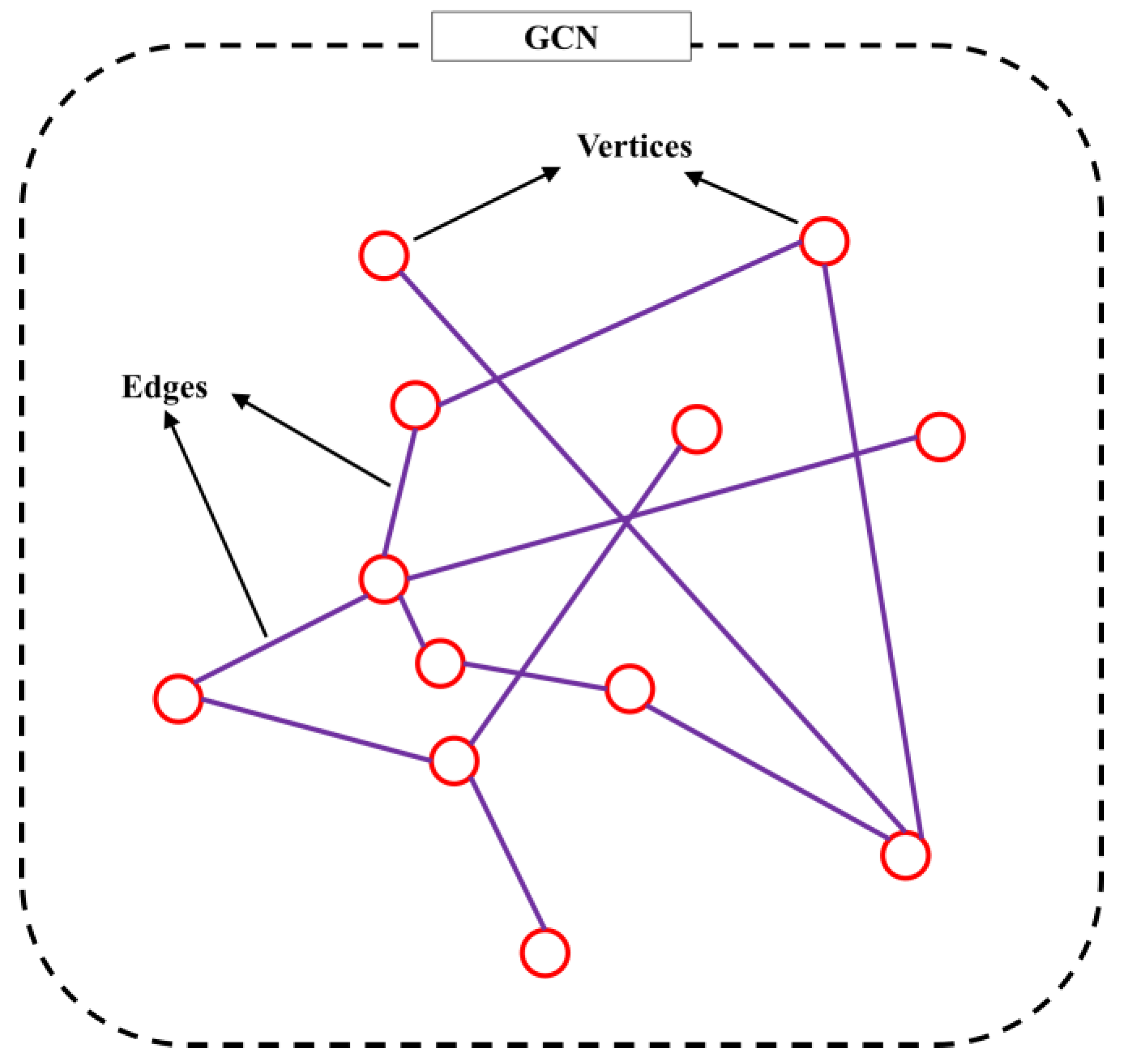
(1) Graph convolutional network (GCN): The GCN [30] works based on defining graphs and relationships among samples in a non-Euclidean space (Figure 2). This provides a helpful tool for considering medium- and long-range relations between pixels rather than only considering short-range relations like convolutional networks. In other words, instead of considering spatial correlation, feature-based relations are considered through an adjacency matrix.
A graph can be defined as G(V, E), where V and E donate a set of vertices and edges, respectively. Vertices indicate input data samples, while edges represent similarities between any two vertices. The edges are defined based on the adjacency matrix (A). It is a symmetric N × N matrix, where N is the number of pixels (nodes) and represents the relationship between each pair of pixels by weights between 0 and 1. Radial basis function (RBF) can be used to calculate the adjacency matrix.
A i , j = exp   ( x i x j 2 σ 2 )
where xi and xj are the feature vector corresponding to vertices vi and vj and σ is the control parameter of the RBF. Accordingly, the normalized graph Laplacian matrix L is represented using diagonal matrix D as follows [40]:
D i , j = j A i , j
L = I D 1 / 2   A   D 1 / 2
where I is an identity matrix. Spectral decomposition on L can be performed on L as follows:
L = U   Λ   U T
where U and Λ are orthogonal eigenvector matrix and diagonal eigenvalues of L, which is the basis function of Fourier transform of feature vector f of each node. The convolution on a graph G can be defined as
G [ f     g θ ]   =   U   g θ   U T   f
where gθ(Λ) is a filter in the Fourier domain that represents the function of eigenvalues (Λ) of L considering the variable θ. The Kth order truncated expansion of Chebyshev polynomials is used to alleviate the computational cost of convolutional on a graph [41].
G [ f     g θ ]     k = 0 K θ k   T k   ( L ˜ ) f
where θ k is the vector of Chebyshev coefficients and Tk donates Chebyshev polynomials. Normalized L ˜ is scaled as L ˜ = 2   L   / λ m a x I . Eventually, Equation (6) can be simplified by considering K = 1 and λmax = 2:
G [ f     g θ ]     θ ( I + D 1 / 2   A   D 1 / 2 ) f .
Regarding Equation (7), the propagation rule for GCNs is defined as follows:
H l + 1 =   h   ( D ˜ 1 / 2   A ˜   D ˜ 1 / 2   H l   w l   + b l )
where adjacency matrix A and D are renormalized as A ˜ = A + I and D ˜ i , j = j A ˜ i , j . Meanwhile, wl, bl, and h() are weight matrix, bias matrix, and activation function. The output of lth and (l + 1)th layers are also indicated by Hl and Hl+1.
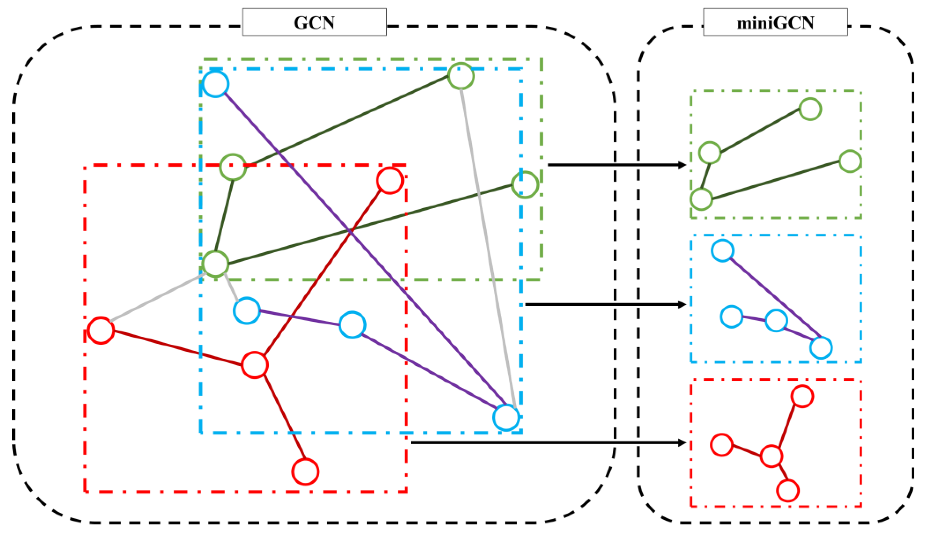
(2) miniGCN overview: Because of the size of the adjacency matrix, GCNs have a substantial computational cost for large graphs. miniGCN [36], which takes advantage of minibatch processing in a batchwise fashion (similar to CNNs), is a feasible solution to the high computational cost issue. For the construction of minibatches, a random node sampler of size M is generated from a full graph G with N nodes on the labeled set (M << N) (Figure 3). In each epoch, the sampler is first applied to the graph until all nodes are sampled, resulting in the generation of subgraphs (Gs):
G   =   { G s   =   ( V s , E s ) | s   =   1 ,   ,   N / M }
where ⌈⌉ is ceiling operator. Consequently, the miniGCN update rule for one batch can be represented as follows:
H ˜ s l + 1 = h   ( D ˜ s 1 / 2   A ˜ s   D ˜ s 1 / 2 H s l   w l + b s l )
where s denotes the sth subgraph as well as the sth batch. The final output in the (l + 1)th layer is calculated.
H l + 1   = [ H ˜ 1 l + 1 ,   ,   H ˜ s l + 1 ,   ,   H ˜ N / M l + 1 ]
The primary difference between this batch procedure and that used in CNNs is that the adjacency matrix of each batch must be reformed after each sampling. The miniGCN model can consider the relationship between pixels using an adjacency matrix, regardless of their distance. While selecting random batchwise samples in each epoch decreases computational cost, it also makes the model compatible with batchwise CNN models and can be integrated with them.

3. The Proposed Method

3.1. PolSAR Feature Extraction

The acquired feature extraction techniques for feeding the proposed network’s spatial and polarimetric channels are defined in the following subsections. As spatial characteristics, Pauli RGB and four-component Yamaguchi decomposition algorithms are defined first. Then, roll-invariant and hidden polarimetric features are explained.
(1) Pauli and decomposition features: The Pauli RGB image is a decomposition approach produced based on scattering matrix S for visualizing PolSAR imagery. The scattering matrix for a full polarized SAR image is defined as follows:
S = [ S H H S H V S V H S V V ]
The scattering matrix is symmetrical (SHV = SVH) in case of satisfying the reciprocity theorem. It can be represented in a way to highlight specific scattering mechanisms:
k = ( 1 / 2 )   [ S H H   +   S V V     S H H     S V V     2 S H V ] T   =   [ a 1     a 2     a 3 ] T
Accordingly, red, green, and blue bands of a false-color Pauli RGB image would be deemed |a2|2 (SHHSVV), |a3|2 (2SHV), and |a1|2 (SHH + SVV). This pseudo-colored image is more human-desirable and in close harmony with natural colors [42], making it easier to consider spatial characteristics such as other colored images. The Coherency matrix T3 can be obtained as follows:
T 3 = ( 1 / L )   i = 1 L k i k i H   =   [ T 11   T 22   T 33 ]
where H donates the complex conjugate transpose, ki is the ith sample of Pauli scattering vector (k), and L indicates the number of looks.
Four-component Yamaguchi decomposition technique decomposes T3 into the four scattering powers of surface (Ps), double-bounce (Pd), volume (Pv), and helix scattering (Ph) [39]. This decomposition is valuable for characterizing urban man-made targets, owing to the helix scattering component that emerges in heterogenous areas [9].
(2) Polarimetric descriptors: To consider the polarimetric characteristics of PolSAR images, roll-invariant and hidden features [25] are deployed. As a result, total backscattering power SPAN is defined as follows:
SPAN = |SHH|2 + 2|SHV|2 + |SVV|2
The coherency matrix can be decomposed based on eigenvalues and eigenvectors, as follows:
T 3   =   U 3   [ λ 1 0 0 0 λ 2 0 0 0 λ 3 ] U 3 H ,         λ 1     λ 2     λ 3
where λ1, λ2, and λ3 are eigenvalues and U3 comprises eigenvectors of the coherency matrix. Accordingly, Cloude–Pottier decomposition components [43], including entropy (H), mean alpha angle ( α ¯ ), and anisotropy (A) are derived.
P i = λ i n = 1 3 λ n ,           i   =   1 ,   2 ,   3
H = n = 1 3 p i log 3 p i
α ¯ = i = 1 3 p i α i
A = λ 2 λ 3 λ 2 + λ 3
In order to leverage the rotation characteristics of PolSAR image, Chen, et al. [44] proposed a method for extending polarimetric features to the rotation domain along the radar line of sight and, accordingly, derived the null angle θnull. The null angles of θnull_Re[T12] and θnull_Im[T12] are highly sensitive to various land covers, which offers a lot of potential for PolSAR classification. These two null angles are presented as follows:
θ null _ Re [ T 12 ] = 1 2 Angle { Re [ T 13 ]   +   j   Re [ T 12 ] } = 1 2 Angle { Re [ ( S HH + S VV )   S H V * ] + j   1 2   ( | S V V | 2 | S H H | 2 ) }
θ null _ Im [ T 12 ] = 1 2 Angle { Im [ T 13 ]   +   j   Im [ T 12 ] } = 1 2 Angle { Im [ ( S HH + S VV )   S H V * ] + j   Im [ S H H S V V * ] }
where Re[] and Im[] get real and imaginary parts, respectively. In contrast, The Angle [] operator acquires phase in complex axis and range of [−π, π].
The six features of SPAN, H, α ¯ , A, θnull_Re[T12], and θnull_Im[T12] are considered for representing and modeling polarimetric characteristics of PolSAR images.

3.2. Dual-Branch FuNet Architecture

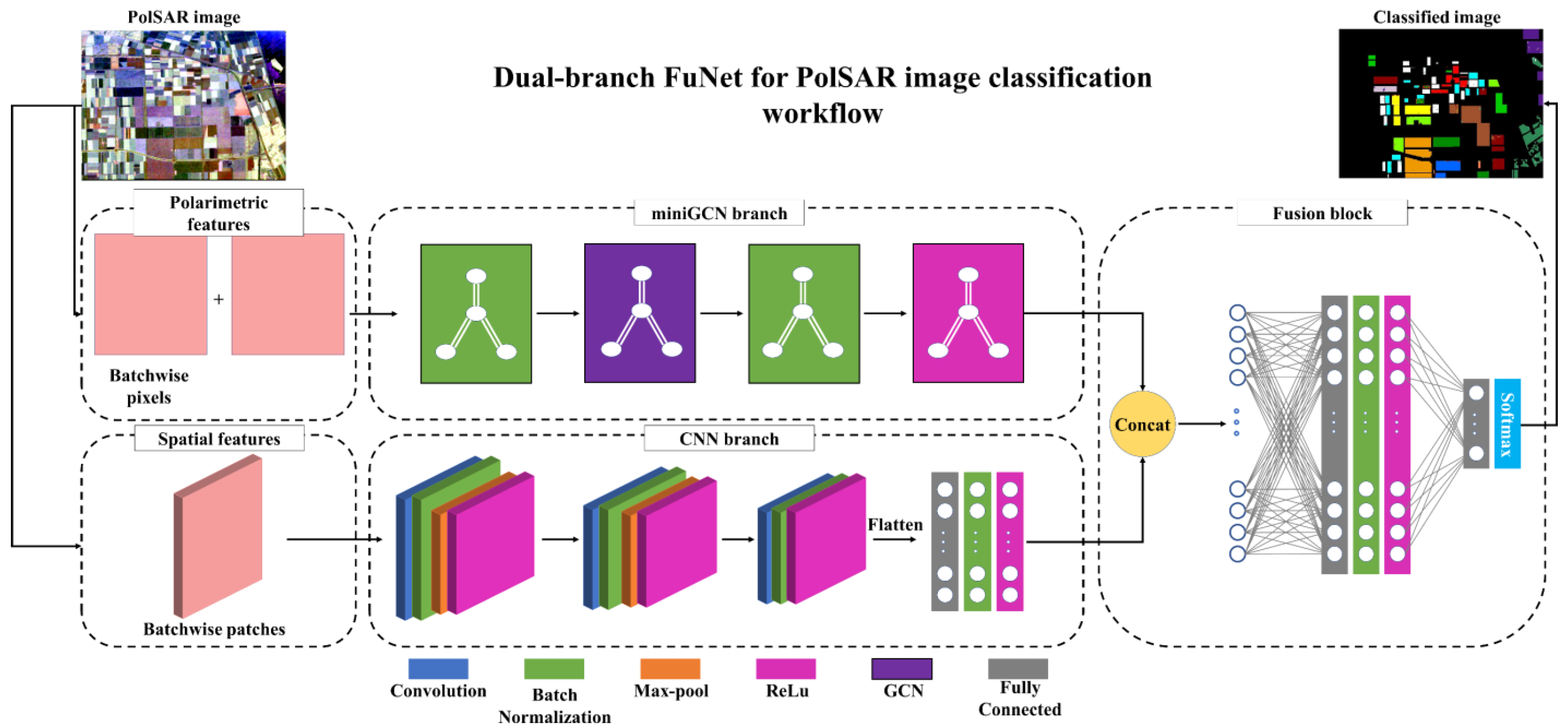
In this study, a dual-branch fusion of miniGCN and CNN networks (FuNet) is proposed for PolSAR image classification, and the framework is depicted in Figure 4. The spatial and polarimetric features of the PolSAR image are inputs for the proposed model. These two sets of PolSAR features are then fed to the CNN and miniGCN, which can extract additional information. The CNN branch leverages the contextual information extraction ability of convolutional kernels, and the miniGCN has the ability to find similarities (such as similarities in polarimetric features) with graphs.
The combination of these two models would help the network make the most of polarimetric data. Therefore, rather than utilizing only the spatial potential of convolutional networks in either one- or two-branch architectures, polarimetric features are deployed in a dual-branch architecture using miniGCN and CNN models. It should be noted that GCN models cannot be fused with CNNs due to their pixel-based structure. As a result, the so-called miniGCN is used to obtain GCN capability in a batchwise strategy.
The proposed network uses spatial and polarimetric features of the PolSAR image as inputs to the CNN and miniGCN branches, respectively. The miniGCN branch consists of a batchwise GCN block. This block is fed by batchwise pixels and an adjacency matrix, which represent nodes and edges of the graph, respectively. In other words, polarimetric features are considered nodes, and the adjacency matrix indicates the relationship between the nodes (edges).
Meanwhile, the CNN branch comprises three two-dimensional convolutional layers and an FC layer. The first two convolutions are followed by maxpooling (pooling size of 2 and stride 2). The FC layer aims to reshape the output of the last convolution to a one-dimensional vector to be concatenated with miniGCN output. The fused output will then be fed to two FC layers to further deepen the network and prepare concatenated features to pass through a Softmax classifier and perform classification. Moreover, a dropout with a 0.5 ratio is applied to the last FC layer to mitigate the overfitting effect.

4. Experiments

4.1. Data Description

The proposed method for PolSAR classification is evaluated in this section, adopting two airborne synthetic aperture radar (AIRSAR) benchmark datasets. Details of the utilized dataset are described as follows:
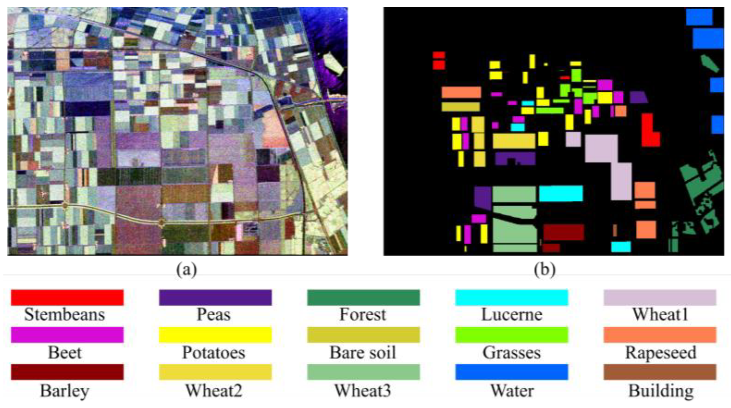
(1) AIRSAR Flevoland data: The Flevoland L-band full polarimetric dataset was acquired by the NASA/JPL AIRSAR platform in 1989 over Flevoland, Netherland. The image size is 750 × 1024 pixels, with 157,296 labeled pixels representing 15 different land cover categories in the ground truth (GT) retrieved from Zhang, et al. [26]. Table 1 lists these land cover categories’ names and sizes (for train and whole GT samples). Figure 5a,b show the Pauli RGB pseudo-color image and GT. The image has a resolution of 6.6 meters (m) in range and 12.1 m in the azimuth direction.
(2) AIRSAR San Francisco data: The San Francisco data also comprise an L-band full polarimetric image captured by the AIRSAR platform in 1989 over San Francisco, USA. The image has a resolution of 900 × 1024 pixels and 802,302 GT labeled pixels, with five land cover categories. The GT is accessible from [45]. Details of GT categories’ names and sizes (for train and whole sample) are compared in Table 2. Figure 6a,b represent the San Francisco image’s Pauli RGB and GT. The spatial resolution of the image is 10 in both directions.
As a preprocessing step, a refined Lee filter with a 7 × 7 window size is applied to both AIRSAR images to reduce the influence of speckle [46].

4.2. Experimental Design

In the current study, a patch-size of 15 × 15 is considered for CNN-based networks since this patch size has been established as the optimal quantity for 2D-CNN classification of AIRSAR datasets [27]. The training samples are randomly chosen from labeled data, with a ratio of 1%. The network’s hyperparameters are as follows: the training epochs are 300, and the batch sizes are 64. Batch normalization is used with a momentum parameter of 0.9. In addition, the base learning rate (LR) of 0.01 is considered. The LR is dynamically updated every 50 epochs by multiplying the base LR by √(1 − iteration/(maximum iteration)). In order to reduce overfitting, L2-norm regularization is obtained (e.g., 0.001). The hyperparameters are set over a grid search. The architecture of the proposed network is illustrated in Table 3. The input of the CNN branch is patchwise, represented by a four-dimensional matrix with the size of N × 15 × 15 × 7, where N is the size of the PolSAR image, 15 × 15 is the patch size, and 7 is the number of spatial features. The input size of miniGCN for the six polarimetric features is N × 6. In addition, a N × N adjacency matrix is considered in the graph model.
Several state-of-the-art classification approaches, including support vector machine (SVM), random forest (RF), 1D-CNN, 2D-CNN, miniGCN, and FuNet, are compared to the proposed method (dual-branch FuNet). SVM with RBF kernel function, RF with 200 decision and 1D-CNN, with two convolutional layers with filter sizes of 120 (with ReLU) and the number of classes (with Softmax), utilized classical classification methods. 2D-CNN with an almost similar structure to [25] is acquired, with the exception of additional L2-norm regularization (same as the proposed network), resulting in identical convolutional blocks with the proposed network’s CNN branch. The utilized miniGCN comprises two graph convolutional layers, the first of which has a size of 120 (similar to the miniGCN branch of the proposed network), and the second one has the same size as the number of classes, which is followed by a Softmax. The FuNet network design is similar to that of the proposed dual-branch method, with polarimetric features given to both miniGCN and CNN branches.
In order to evaluate and compare the performance of methods, overall accuracy (OA) and kappa coefficient (K) are adopted.

4.3. Parameter Setting, Adjacency Matrix

The adjacency matrix significantly impacts the quality of the proposed method’s miniGCN branch. As a result, optimum parameters for the construction of the adjacency matrix, including the number of neighbors (K) and RBF function width (σ), are required.
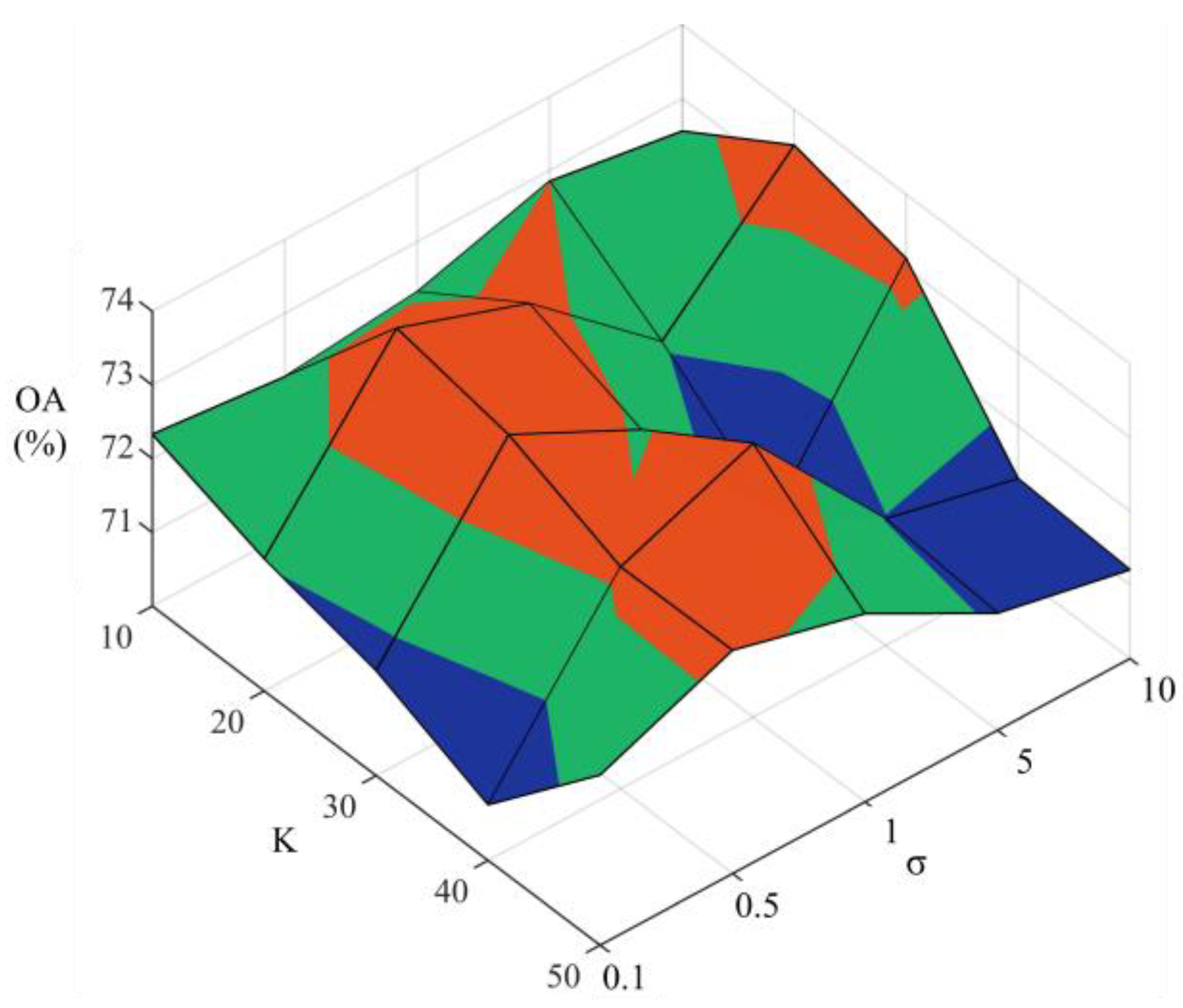
A grid search was conducted on Flevoland data to identify the suitable parameters using the miniGCN network (Figure 7). The overall accuracy of miniGCN varies substantially over the search range. While K = 20 and σ = 0.5 yield the highest OA, the OAs are not stable near those values. The most stable outcomes are obtained using K = 10 and σ = 1. In other words, the lowest standard deviations (SD) were 0.2% and 0.5%, at K = 10 and σ = 1, respectively. SDs for different sets of parameters, in contrast, are not less than 1% and 0.7% (for each K and σ). Eventually, (K = 10, σ = 1) is taken into consideration for the proposed network classification.

4.4. Effectiveness Evaluation

To indicate consistency of the proposed method, it was implemented five times, and the average of the results were considered for further evaluation. The processing stage was conducted using an 8 GB memory Intel Core i7-7500U processor. The training process for 300 epochs of the AIRSAR Flevoland dataset with 1% sampling ratio (1579 samples) was 1985 seconds.
The convergence of losses and accuracies of the dual-branch FuNet model for AIRSAR Flevoland are shown in Figure 8. After 150 epochs, the loss of both training and test sets become almost steady, indicating the effectiveness of the network’s training process. Eventually, the training accuracy reaches 100%, while the test set becomes approximately 98%.

4.5. Experiments on AIRSAR Datasets

The proposed dual-branch FuNet land cover classification results are compared to several state-of-the-art methods, including SVM, RF, 1D-CNN, 2D-CNN, miniGCN, and FuNet, over AIRSAR Flevoland and AIRSAR San Francisco. To establish a fair comparison, similar random samples (with 1% TR) are selected, and the average performance of each network’s five-time running is represented.
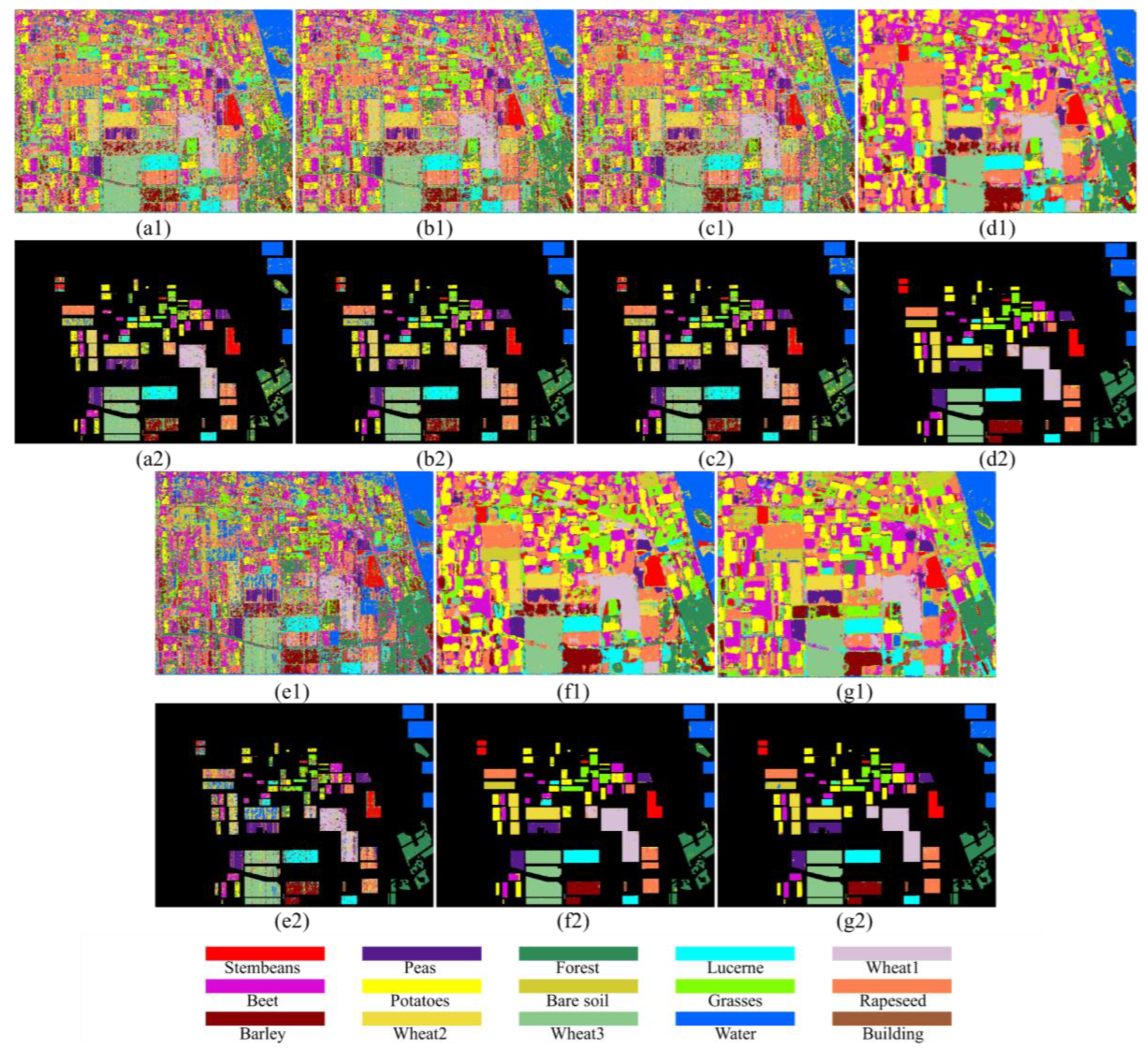
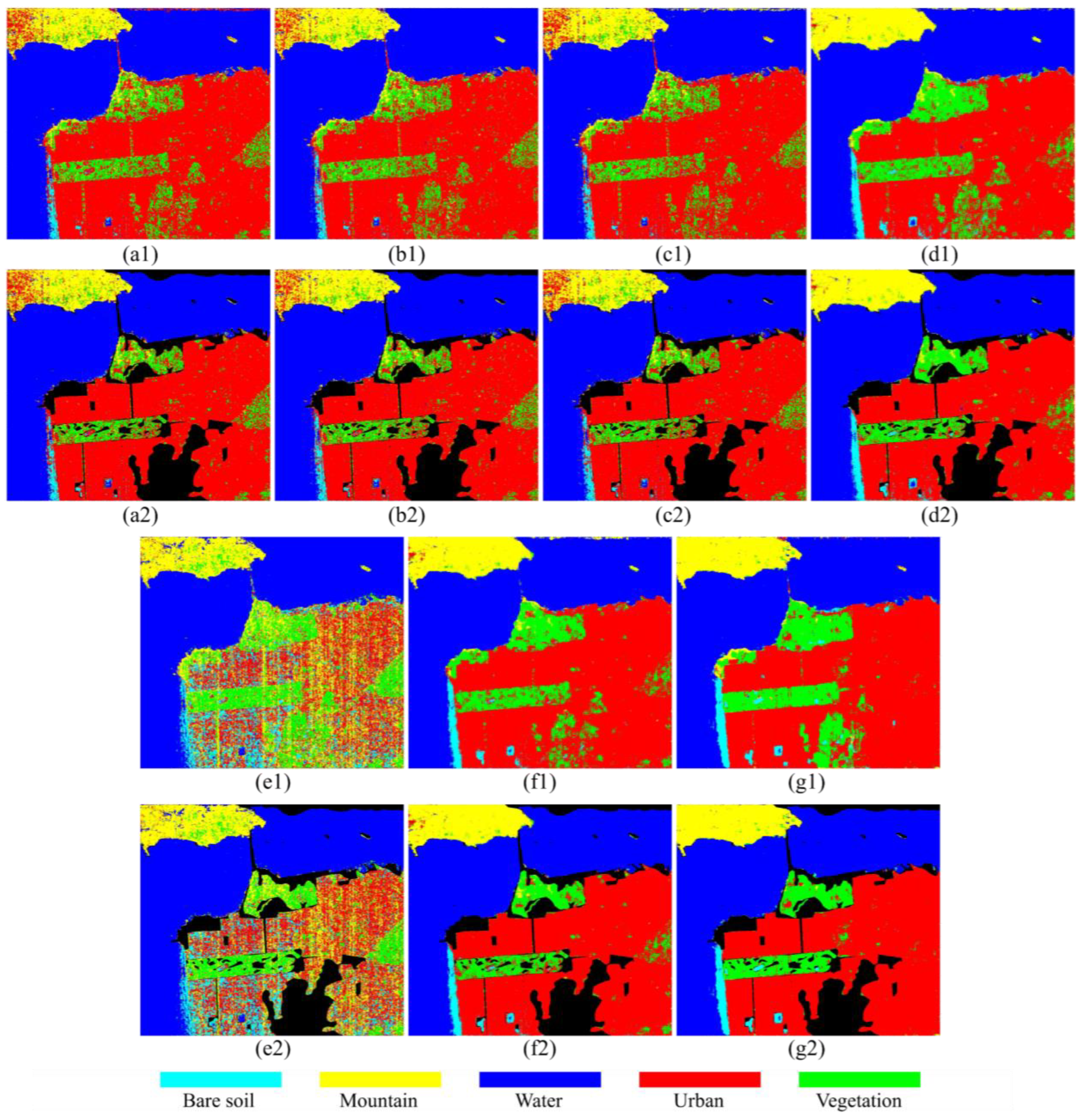
In Figure 9 and Figure 10, the proposed method’s classified maps are visually compared to the six state-of-the-art methods for the entire image and the labeled regions, demonstrating that the FuNet network and its dual-branch version produce significantly smoother and more satisfying results for both datasets. Furthermore, in the Flevoland case, classical methods and miniGCN classification maps are noisy and seem to be impacted by speckle, whereas networks using convolutional layers (including 2D-CNN, FuNet, and dual-branch FuNet) produce smoother results. Similarly, in the case of the San Francisco data, classical approaches and miniGCN yield noisy and misclassified results, particularly in the mountain and urban areas.
Per-class OA, overall OA, and kappa coefficient for the methods mentioned above are compared to the proposed one in Table 4 and Table 5. It can be observed that classical methods of SVM, RF, and 1D-CNN have performed almost similarly, attaining OAs of 78–80% and approximately 91% for Flevoland and San Francisco, respectively. Meanwhile, the 2D-CNN achieved high OA and K, benefiting from its potential to extract 2D features and the use of neighboring pixels’ information. Accordingly, it reached the highest OA for bare soil and grass classes in the Flevoland dataset.
The miniGCN, which is powered by the graph’s long-range similarity detection ability, showed overall poor performance compared to the classical networks. The reason for this performance is graph edges or adjacency matrix, which connects pixels based on their similarities in input features rather than target classes. Therefore, in classes such as urban areas in the AIRSAR San Francisco dataset that contain mixed pixels (such as vegetation coverage), the output is affected by the similarities considered in the adjacency matrix. In contrast, in classes with fewer mixed pixels (such as building in Flevoland), even with a small number of training samples (five for the building class), the miniGCN performed well. It also achieved the highest OA in the water class. Furthermore, in the case of the San Francisco image, the miniGCN surpasses classical approaches (except in urban class).
The FuNet model outperforms the abovementioned methods by combining the convolutional advantage of 2D-CNN with the ability of graphs to consider the long-range relationships. Using both polarimetric and spatial features of PolSAR images in the dual-branch FuNet model further improves its performance compared to the one-branch model. Eventually, dual-branch FuNet achieved OA and K of 97.84% and 97.64% for Flevoland and 98.09% and 97% for San Francisco. Flevoland data had the foremost OAs for forest, beet, rapeseed, building, and all three wheat classes. Moreover, it is the only model that achieved above 90% OAs for all classes, with 91.93% for building as the lowest per-class OA. Meanwhile, for the San Francisco case, four of the existing five classes, including bare soil, mountain, urban, and vegetation, obtained their maximum OAs using the proposed dual-branch network.

4.6. Performance Analyses with Different Training Sampling Rates

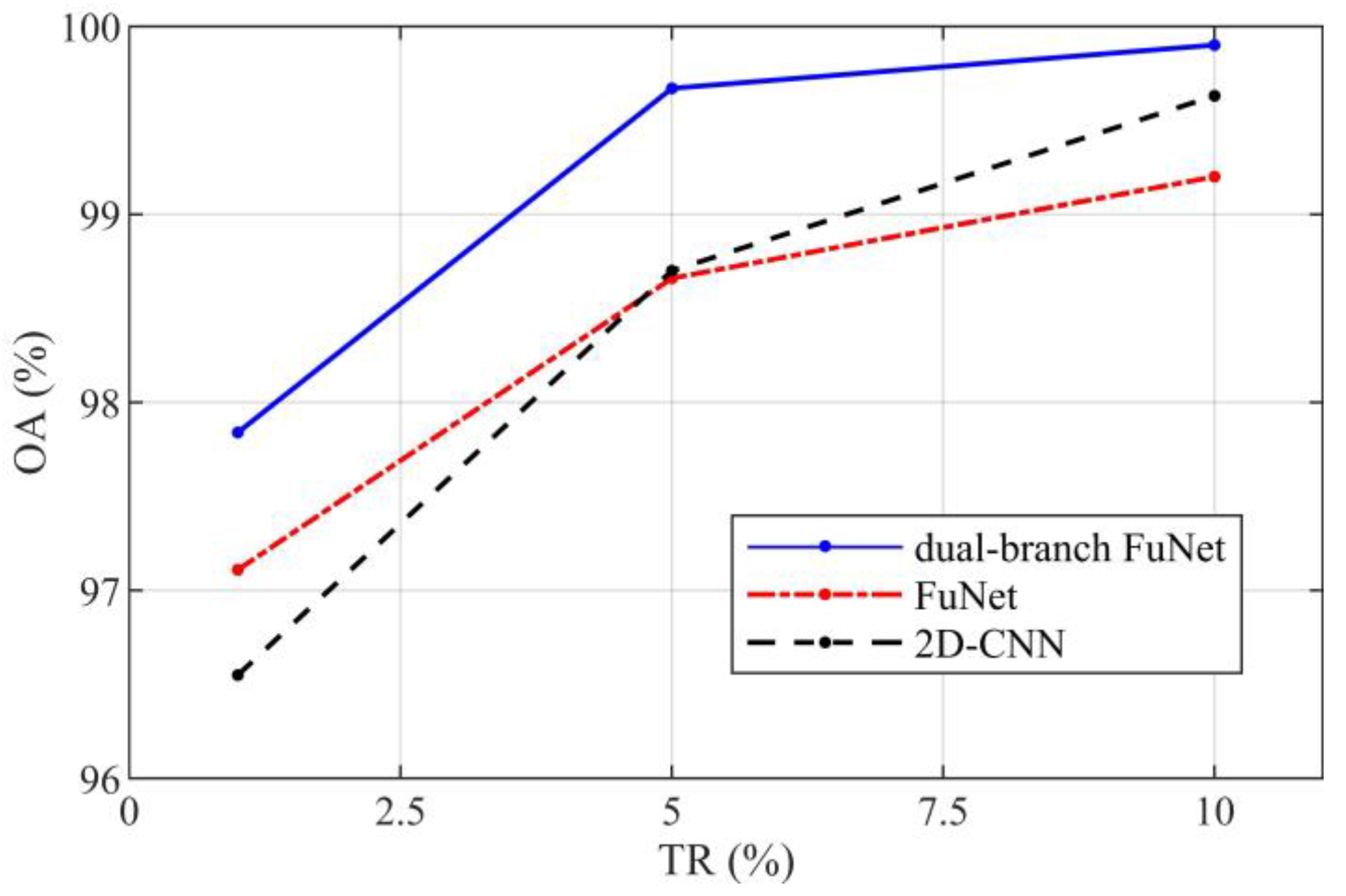
In general, supervised classification methods work with a limited number of training samples; thus, their ability to discriminate varied land covers with restricted sample data is crucial. Accordingly, the effect of various training sample ratios (TRs) on the performance of the proposed method is compared to that of the other methods over the Flevoland data. Table 6 depicts classification OAs of 1%, 5%, and 10% TRs. The result indicates that the proposed dual-branch FuNet achieved the highest OAs with different TRs, followed by 2D-CNN and FuNet.
To offer a clear visual comparison, Figure 11 illustrates the performance of the three superior networks. It can be observed that with an adequate sampling ratio of 10%, 2D-CNN outperforms FuNet and is slightly lower than the dual-branch network. When TR is reduced to 5%, the OAs of 2D-CNN and FuNet fall by 0.93% and 0.54%, whereas that of the dual-branch decreases marginally (0.23%). Considering 1% TR, 2D-CNN degrades significantly (2.58%), whereas the proposed dual-branch and its one-branch version of FuNet have more stable results. Overall, the dual-branch FuNet shows the least sensitivity to changes in training sample ratios and achieves the highest OAs.

4.7. Comparison with Other Studies

The proposed method is compared to some published PolSAR classification techniques to provide a more comprehensive verification. For a fair comparison, using similar benchmark data and ground-truth (GT) is recommended. Accordingly, AIRSAR Flevoland benchmark data, which has been widely deployed in previous studies, is regarded for comparison. It should be noted that some of the other papers have employed different GTs with different random training samples, which might impact the obtained result.
The PolSAR classification approaches of complex-valued CNN (CV-CNN) [26], dual-branch deep CNN (dual-branch DCNN) [27], 2D-CNN [25], multichannel fusion CNN (MCFCNN) [28], and semi-supervised multiscale evolving weighted GCN (MEWGCN) [47] are the ones compared with the proposed FuNet and dual-branch FuNet (Table 7).
It should be noted that several GTs with varied numbers of labeled points are utilized, with only CV-CNN sharing the same GT as the current study. With an identical GT, CV-CNN showed poor performance, with 1% TR, and inferior OA, with 5% and 10%. When using a limited amount of training data (1%), this method has even lower performance compared to the SVM and RF with proposed input features. This indicates the importance of model input parameters and how extracted spatial and polarimetric features can boost the classifier performance, particularly with limited training data. The dual-branch method in Gao, et al. [27] produces promising results (98.53% OA) with a sufficient sampling rate of 75%. However, it is still low compared to the proposed method’s 5% and 10%. The architecture of the proposed dual-branch model (using a miniGCN branch) aside from the modified input features are the main factors for improving dual-branch method classification ability with low TR. Although the polarimetric feature-driven 2D-CNN, MCFCNN, and MEWGCN produced satisfactory accuracies, they still have lower OAs compared to the proposed dual-branch FuNet.

5. Conclusions

Since PolSAR images’ characteristics vary from those of optical images, a specialized approach for extracting spatial information is required. Combining both spatial and polarimetric features allows us to fully consider the rich information of PolSAR images. Accordingly, a dual-branch network utilizing DCNN and miniGCN was developed in the current study to make the most of PolSAR features.
Deep convolutional models can consider spatial characteristics utilizing neighborhood information, for which, in the current study, Pauli RGB and four-component Yamaguchi decomposition were driven to provide spatial features of the PolSAR image. In contrast, roll-invariant and hidden polarimetric features were obtained to feed the miniGCN. miniGCN is a batchwise version of GCN that can cooperate with batchwise CNN and considers long-range similarities through an adjacency matrix, while it requires significantly lower computational cost. Eventually, the DCNN and miniGCN were fused in the proposed dual-branch network, called dual-branch FuNet, to discriminate PolSAR classes.
The proposed classifier outperforms several state-of-the-art models over AIRSAR Flevoland and San Francisco datasets, reaching above 97% OA for both cases. When compared to traditional approaches (SVM, RF, and 1D- and 2D-CNN), improvements ranged from 1.3% to 19.27% (OA). Furthermore, the dual-branch strategy outperforms the simple one-branch network by 0.73% to 1.82% in terms of OA. The investigated dual-branch network offers a robust technique to deal with different sampling rates (1 to 10%) and produces a stable result, even with the small-labeled sample, i.e., between 97.8% and 99.9% OA.

Author Contributions

Conceptualization, M.M.; Supervision, M.M.; Formal Analysis, A.R. and M.M.; Data Collection, A.R.; Visualization, A.R.; Writing—Original Draft Preparation, A.R.; Writing—Review and Editing, A.R., M.M., B.B., B.S. and F.M. All authors have read and agreed to the published version of the manuscript.

Funding

This study was funded by the Natural Sciences and Engineering Research Council (NSERC) Discovery under Grant to M. Mahdianpari (Grant No. RGPIN-2022-04766).

Data Availability Statement

The original PolSAR data are openly available and can be found here: https://ietr-lab.univ-rennes1.fr/polsarpro-bio/sample_datasets/. The data presented in this study are available on reasonable request from the corresponding author.

Conflicts of Interest

The authors declare no conflict of interest.

References

  1. Ren, B.; Hou, B.; Zhao, J.; Jiao, L. Sparse subspace clustering-based feature extraction for PolSAR imagery classification. Remote Sens. 2018, 10, 391. [Google Scholar] [CrossRef] [Green Version]
  2. Zhang, Q.; Wei, X.; Xiang, D.; Sun, M. Supervised PolSAR Image Classification with Multiple Features and Locally Linear Embedding. Sensors 2018, 18, 3054. [Google Scholar] [CrossRef] [Green Version]
  3. Zhong, N.; Yang, W.; Cherian, A.; Yang, X.; Xia, G.-S.; Liao, M. Unsupervised classification of polarimetric SAR images via Riemannian sparse coding. IEEE Trans. Geosci. Remote Sens. 2017, 55, 5381–5390. [Google Scholar] [CrossRef]
  4. Doulgeris, A.P.; Anfinsen, S.N.; Eltoft, T. Automated non-Gaussian clustering of polarimetric synthetic aperture radar images. IEEE Trans. Geosci. Remote Sens. 2011, 49, 3665–3676. [Google Scholar] [CrossRef]
  5. Yin, J.; Liu, X.; Yang, J.; Chu, C.-Y.; Chang, Y.-L. PolSAR image classification based on statistical distribution and MRF. Remote Sens. 2020, 12, 1027. [Google Scholar] [CrossRef] [Green Version]
  6. Jafari, M.; Maghsoudi, Y.; Zoej, M.J.V. A new method for land cover characterization and classification of polarimetric SAR data using polarimetric signatures. IEEE J. Sel. Top. Appl. Earth Obs. Remote Sens. 2015, 8, 3595–3607. [Google Scholar] [CrossRef]
  7. Freeman, A.; Durden, S.L. A three-component scattering model for polarimetric SAR data. IEEE Trans. Geosci. Remote Sens. 1998, 36, 963–973. [Google Scholar] [CrossRef] [Green Version]
  8. Krogager, E. New decomposition of the radar target scattering matrix. Electron. Lett. 1990, 26, 1525–1527. [Google Scholar] [CrossRef]
  9. Yamaguchi, Y.; Moriyama, T.; Ishido, M.; Yamada, H. Four-component scattering model for polarimetric SAR image decomposition. IEEE Trans. Geosci. Remote Sens. 2005, 43, 1699–1706. [Google Scholar] [CrossRef]
  10. Fan, J.; Wang, X.; Wang, X.; Zhao, J.; Liu, X. Incremental wishart broad learning system for fast PolSAR image classification. IEEE Geosci. Remote Sens. Lett. 2019, 16, 1854–1858. [Google Scholar] [CrossRef]
  11. Lee, J.-S.; Grunes, M.R.; Kwok, R. Classification of multi-look polarimetric SAR imagery based on complex Wishart distribution. Int. J. Remote Sens. 1994, 15, 2299–2311. [Google Scholar] [CrossRef]
  12. Chaudhari, N.; Mitra, S.K.; Mandal, S.; Chirakkal, S.; Putrevu, D.; Misra, A. Edge-Preserving classification of polarimetric SAR images using Wishart distribution and conditional random field. Int. J. Remote Sens. 2022, 43, 2134–2155. [Google Scholar] [CrossRef]
  13. Khosravi, I.; Safari, A.; Homayouni, S.; McNairn, H. Enhanced decision tree ensembles for land-cover mapping from fully polarimetric SAR data. Int. J. Remote Sens. 2017, 38, 7138–7160. [Google Scholar] [CrossRef]
  14. Qi, Z.; Yeh, A.G.-O.; Li, X.; Lin, Z. A novel algorithm for land use and land cover classification using RADARSAT-2 polarimetric SAR data. Remote Sens. Environ. 2012, 118, 21–39. [Google Scholar] [CrossRef]
  15. Zhang, L.; Zou, B.; Zhang, J.; Zhang, Y. Classification of polarimetric SAR image based on support vector machine using multiple-component scattering model and texture features. EURASIP J. Adv. Signal Process. 2009, 2010, 1–9. [Google Scholar] [CrossRef] [Green Version]
  16. Tao, C.; Chen, S.; Li, Y.; Xiao, S. PolSAR land cover classification based on roll-invariant and selected hidden polarimetric features in the rotation domain. Remote Sens. 2017, 9, 660. [Google Scholar] [CrossRef] [Green Version]
  17. Zhou, Y.; Wang, H.; Xu, F.; Jin, Y.-Q. Polarimetric SAR image classification using deep convolutional neural networks. IEEE Geosci. Remote Sens. Lett. 2016, 13, 1935–1939. [Google Scholar] [CrossRef]
  18. Zhang, L.; Ma, W.; Zhang, D. Stacked sparse autoencoder in PolSAR data classification using local spatial information. IEEE Geosci. Remote Sens. Lett. 2016, 13, 1359–1363. [Google Scholar] [CrossRef]
  19. Chen, Y.; Jiao, L.; Li, Y.; Zhao, J. Multilayer projective dictionary pair learning and sparse autoencoder for PolSAR image classification. IEEE Trans. Geosci. Remote Sens. 2017, 55, 6683–6694. [Google Scholar] [CrossRef]
  20. Lv, Q.; Dou, Y.; Niu, X.; Xu, J.; Li, B. Classification of Land Cover Based on Deep Belief Networks Using Polarimetric RADARSAT-2 Data. In Proceedings of the 2014 IEEE Geoscience and Remote Sensing Symposium, Quebec City, QC, Canada, 13–18 July 2014; pp. 4679–4682. [Google Scholar]
  21. Jamali, A.; Mahdianpari, M.; Mohammadimanesh, F.; Bhattacharya, A.; Homayouni, S. PolSAR image classification based on deep convolutional neural networks using wavelet transformation. IEEE Geosci. Remote Sens. Lett. 2022, 19, 4510105. [Google Scholar] [CrossRef]
  22. Xie, W.; Jiao, L.; Hua, W. Complex-Valued Multi-Scale Fully Convolutional Network with Stacked-Dilated Convolution for PolSAR Image Classification. Remote Sens. 2022, 14, 3737. [Google Scholar] [CrossRef]
  23. Hua, W.; Xie, W.; Jin, X. Three-Channel Convolutional Neural Network for Polarimetric SAR Images Classification. IEEE J. Sel. Top. Appl. Earth Obs. Remote Sens. 2020, 13, 4895–4907. [Google Scholar] [CrossRef]
  24. Wang, H.; Xing, C.; Yin, J.; Yang, J. Land Cover Classification for Polarimetric SAR Images Based on Vision Transformer. Remote Sens. 2022, 14, 4656. [Google Scholar] [CrossRef]
  25. Chen, S.-W.; Tao, C.-S. PolSAR image classification using polarimetric-feature-driven deep convolutional neural network. IEEE Geosci. Remote Sens. Lett. 2018, 15, 627–631. [Google Scholar] [CrossRef]
  26. Zhang, Z.; Wang, H.; Xu, F.; Jin, Y.-Q. Complex-valued convolutional neural network and its application in polarimetric SAR image classification. IEEE Trans. Geosci. Remote Sens. 2017, 55, 7177–7188. [Google Scholar] [CrossRef]
  27. Gao, F.; Huang, T.; Wang, J.; Sun, J.; Hussain, A.; Yang, E. Dual-branch deep convolution neural network for polarimetric SAR image classification. Appl. Sci. 2017, 7, 447. [Google Scholar] [CrossRef] [Green Version]
  28. Wang, Y.; Cheng, J.; Zhou, Y.; Zhang, F.; Yin, Q. A Multichannel Fusion Convolutional Neural Network Based on Scattering Mechanism for PolSAR Image Classification. IEEE Geosci. Remote Sens. Lett. 2021, 19, 4007805. [Google Scholar] [CrossRef]
  29. Shang, R.; Wang, J.; Jiao, L.; Yang, X.; Li, Y. Spatial feature-based convolutional neural network for PolSAR image classification. Appl. Soft Comput. 2022, 123, 108922. [Google Scholar] [CrossRef]
  30. Kipf, T.N.; Welling, M. Semi-supervised classification with graph convolutional networks. arXiv 2016, arXiv:1609.02907. [Google Scholar]
  31. Qin, A.; Shang, Z.; Tian, J.; Wang, Y.; Zhang, T.; Tang, Y.Y. Spectral–spatial graph convolutional networks for semisupervised hyperspectral image classification. IEEE Geosci. Remote Sens. Lett. 2018, 16, 241–245. [Google Scholar] [CrossRef]
  32. Wan, S.; Gong, C.; Zhong, P.; Pan, S.; Li, G.; Yang, J. Hyperspectral image classification with context-aware dynamic graph convolutional network. IEEE Trans. Geosci. Remote Sens. 2020, 59, 597–612. [Google Scholar] [CrossRef]
  33. Ding, Y.; Zhang, Z.; Zhao, X.; Hong, D.; Li, W.; Cai, W.; Zhan, Y. AF2GNN: Graph convolution with adaptive filters and aggregator fusion for hyperspectral image classification. Inf. Sci. 2022, 602, 201–219. [Google Scholar] [CrossRef]
  34. Yao, D.; Zhi-li, Z.; Xiao-feng, Z.; Wei, C.; Fang, H.; Yao-ming, C.; Cai, W.-W. Deep hybrid: Multi-graph neural network collaboration for hyperspectral image classification. Def. Technol. 2022, in press. [CrossRef]
  35. He, X.; Chen, Y.; Ghamisi, P. Dual Graph Convolutional Network for Hyperspectral Image Classification with Limited Training Samples. IEEE Trans. Geosci. Remote Sens. 2021, 60, 5502418. [Google Scholar] [CrossRef]
  36. Hong, D.; Gao, L.; Yao, J.; Zhang, B.; Plaza, A.; Chanussot, J. Graph convolutional networks for hyperspectral image classification. IEEE Trans. Geosci. Remote Sens. 2020, 59, 5966–5978. [Google Scholar] [CrossRef]
  37. Cai, W.; Wei, Z. Remote sensing image classification based on a cross-attention mechanism and graph convolution. IEEE Geosci. Remote Sens. Lett. 2020, 19, 8002005. [Google Scholar] [CrossRef]
  38. Du, X.; Zheng, X.; Lu, X.; Doudkin, A.A. Multisource remote sensing data classification with graph fusion network. IEEE Trans. Geosci. Remote Sens. 2021, 59, 10062–10072. [Google Scholar] [CrossRef]
  39. Yamaguchi, Y.; Sato, A.; Boerner, W.-M.; Sato, R.; Yamada, H. Four-component scattering power decomposition with rotation of coherency matrix. IEEE Trans. Geosci. Remote Sens. 2011, 49, 2251–2258. [Google Scholar] [CrossRef]
  40. Hong, D.; Yokoya, N.; Ge, N.; Chanussot, J.; Zhu, X.X. Learnable manifold alignment (LeMA): A semi-supervised cross-modality learning framework for land cover and land use classification. ISPRS J. Photogramm. Remote Sens. 2019, 147, 193–205. [Google Scholar] [CrossRef]
  41. Hammond, D.K.; Vandergheynst, P.; Gribonval, R. Wavelets on graphs via spectral graph theory. Appl. Comput. Harmon. Anal. 2011, 30, 129–150. [Google Scholar] [CrossRef] [Green Version]
  42. Uhlmann, S.; Kiranyaz, S. Integrating color features in polarimetric SAR image classification. IEEE Trans. Geosci. Remote Sens. 2013, 52, 2197–2216. [Google Scholar] [CrossRef]
  43. Cloude, S.R.; Pottier, E. An entropy based classification scheme for land applications of polarimetric SAR. IEEE Trans. Geosci. Remote Sens. 1997, 35, 68–78. [Google Scholar] [CrossRef]
  44. Chen, S.-W.; Wang, X.-S.; Sato, M. Uniform polarimetric matrix rotation theory and its applications. IEEE Trans. Geosci. Remote Sens. 2013, 52, 4756–4770. [Google Scholar] [CrossRef]
  45. Liu, X.; Jiao, L.; Liu, F. PolSF: PolSAR Image Dataset on San Francisco. arXiv 2019, arXiv:1912.07259. [Google Scholar]
  46. Lee, J.-S.; Grunes, M.R.; De Grandi, G. Polarimetric SAR speckle filtering and its implication for classification. IEEE Trans. Geosci. Remote Sens. 1999, 37, 2363–2373. [Google Scholar]
  47. Ren, S.; Zhou, F. Semi-Supervised Classification for PolSAR Data with Multi-Scale Evolving Weighted Graph Convolutional Network. IEEE J. Sel. Top. Appl. Earth Obs. Remote Sens. 2021, 14, 2911–2927. [Google Scholar] [CrossRef]
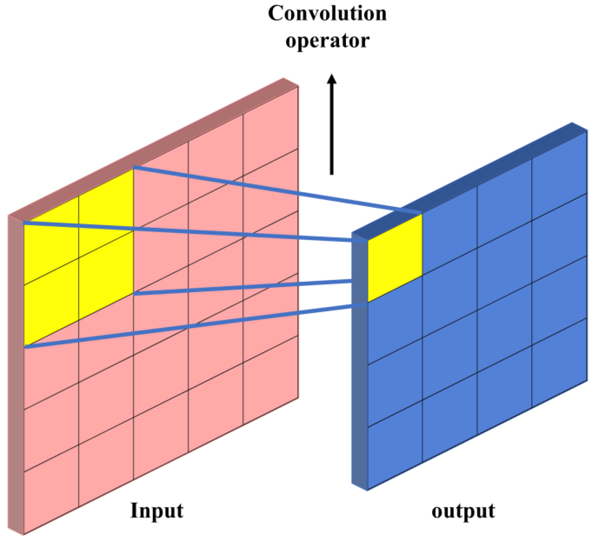
Figure 1. General structure of a convolution (2 × 2 convolutional operator).
Remotesensing 15 00075 g001
Figure 2. General structure of a graph.
Remotesensing 15 00075 g002
Figure 3. Batchwise structure of miniGCN. Three minibatches are considered with the random node sampler size of M = 4, compared to full graph with N = 12 nodes.
Remotesensing 15 00075 g003
Figure 4. The framework of the proposed dual-branch FuNet, including three main steps: polarimetric and spatial feature extraction, miniGCN and CNN layers, and fusion layers leading to a classified PolSAR image.
Remotesensing 15 00075 g004
Figure 5. (a) Pauli RGB and (b) ground truth map of AIRSAR Flevoland data.
Remotesensing 15 00075 g005
Figure 6. (a) Pauli RGB and (b) ground truth map of AIRSAR San Francisco data.
Remotesensing 15 00075 g006
Figure 7. Adjacency matrix parameters (K, σ) impact on classification OA of miniGCN.
Remotesensing 15 00075 g007
Figure 8. (a) Accuracy and (b) loss curves of the dual-branch FuNet model.
Remotesensing 15 00075 g008
Figure 9. AIRSAR Flevoland classification maps of (a1) SVM, (b1) RF, (c1) 1D-CNN, (d1) 2D-CNN, (e1) miniGCN, (f1) FuNet, and (g1) dual-branch FuNet. (a2)–(g2) Masked results according to the ground-truth of (a1)–(g1).
Remotesensing 15 00075 g009
Figure 10. AIRSAR San Francisco classification maps of (a1) SVM, (b1) RF, (c1) 1D-CNN, (d1) 2D-CNN, (e1) miniGCN, (f1) FuNet, and (g1) dual-branch FuNet. (a2)–(g2) Masked results according to the ground-truth of (a1)–(g1).
Remotesensing 15 00075 g010
Figure 11. Classification OAs of superior networks with different training ratios on AIRSAR Flevoland data.
Remotesensing 15 00075 g011
Table 1. Details of classes and training samples for AIRSAR Flevoland data (TR represents training ratio).
Class NumberClass NameTrain NumberSample NumberTR (%)
1Stem beans6261031.015894
2Peas9291111.009768
3Forest15014,9441.003747
4Lucerne9594771.002427
5Wheat17317,2831.000984
6Beet10110,0501.004975
7Potatoes15315,2921.000523
8Bare soil3130781.007147
9Grass6362691.004945
10Rapeseed12712,6901.000788
11Barley7271561.006149
12Wheat210610,5911.00085
13Wheat321421,3001.004695
14Water13513,4761.001781
15Buildings54761.05042
All1579157,2961.00384
Table 2. Details of classes and training samples for AIRSAR San Francisco data (TR represents training ratio).
Class NumberClass NameTrain NumberSample NumberTR (%)
1Bare soil13813,7011.007226
2Mountain62862,7311.0011
3Water3296329,5661.000103
4Urban3428342,7951.000015
5Vegetation53653,5091.001701
All8026802,3021.000371
Table 3. The architecture of the dual-branch FuNet.
LayerCNNminiGCN
Input15 × 15 × 7 (Spatial feature)6 Polarimetric feature
Block 12 × 2 ConvBN
BNGraph Conv
2 × 2 MaxpoolBN
ReLUReLU
Output size8 × 8 × 30120
Block 22 × 2 Conv-
BN-
2 × 2 Maxpool-
ReLU-
Output size4 × 4 × 60-
Block 32 × 2 Conv-
BN-
ReLU-
Output size4 × 4 × 120-
Fully connectedFC Encoder-
BN-
ReLU-
Output size120-
FusionFC Encoder
BN
ReLU
Output size240
OutputFC Encoder
Softmax
Output sizeNumber of classes
Table 4. Detailed classification OAs and K of different algorithms compared to the proposed method on AIRSAR Flevoland. Bold numbers indicate the highest accuracy in each row.
ClassesModels
NameSVMRF1D-CNN2D-CNNminiGCNFuNetDual-Branch FuNet
Stem beans80.9580.9079.5999.4766.3399.4799.35
Peas77.2676.2277.7897.5483.1496.7497.62
Forest77.1385.3676.6596.6996.6296.4398.33
Lucerne83.2384.5681.2897.1181.1297.3594.54
Wheat71.0772.3673.7093.1263.7695.2098.85
Beet77.8079.8583.0894.3471.3994.1898.05
Potatoes72.4272.0676.1993.3449.3897.0397.02
Bare soil66.2668.0081.29100.0056.58100.0094.58
Grass69.3470.3871.8796.4665.1995.9794.25
Rapeseed74.8271.6974.3194.9858.1395.5297.48
Barley70.9976.9678.6798.0983.5498.9097.52
Wheat271.1169.3871.7196.7342.8497.1597.47
Wheat390.1889.6489.8699.6778.3299.2199.75
Water96.4596.7892.9399.0099.9199.0398.94
Buildings65.8268.7977.2880.6883.8686.2091.93
OA (%)78.5779.5579.8196.5472.3297.1197.84
K (%)76.5777.6477.9496.2269.8696.8497.64
Table 5. Detailed classification OAs and K of different algorithms compared to the proposed method on AIRSAR San Francisco. Bold numbers indicate the highest accuracy in each row.
ClassesModels
NameSVMRF1D-CNN2D-CNNminiGCNFuNetDual-Branch FuNet
Bare soil40.8745.6044.2174.0950.6676.2188.76
Mountain73.1076.3273.9296.2582.9895.9297.38
Water98.9898.9098.9599.3999.0699.4999.40
Urban94.8894.4694.9294.9348.3696.8098.68
Vegetation55.8457.5357.4578.0763.7478.5389.36
OA (%)91.3391.5791.5795.3972.9596.2798.09
K (%)86.2286.6586.6292.7962.0594.1497.00
Table 6. Classification OAs with different training ratios on AIRSAR Flevoland data. Bold numbers indicate the highest accuracy in each row.
Training
Ratio (%)
SVMRF1D-CNN2D-CNNminiGCNFuNetDual-Branch FuNet
OA (%)178.5779.5579.8196.5472.3297.1197.84
581.9583.4382.5998.775.5298.6699.67
1083.1684.4583.199.6376.9499.299.9
Table 7. Comparison of classification OAs with other studies on AIRSAR Flevoland data. Bold numbers indicate the highest accuracy in each row.
Training Ratio %CV-CNNDual-Branch2D-CNNMCFCNNMEWGCNProposed
OA (%)16298.53 (75% TR)97.5795.83-97.84
59498.83-99.3999.67
1096.299.3--99.9
Disclaimer/Publisher’s Note: The statements, opinions and data contained in all publications are solely those of the individual author(s) and contributor(s) and not of MDPI and/or the editor(s). MDPI and/or the editor(s) disclaim responsibility for any injury to people or property resulting from any ideas, methods, instructions or products referred to in the content.