Abstract
In today’s accelerating urbanization process, timely and effective monitoring of land-cover dynamics, landscape pattern analysis, and evaluation of built-up urban areas (BUAs) have important research significance and practical value for the sustainable development, planning and management, and ecological protection of cities. High-spatial-resolution remote sensing (HRRS) images have the advantages of high-accuracy Earth observations, covering a large area, and having a short playback period, and they can objectively and accurately provide fine dynamic spatial information about the land cover in urban built-up areas. However, the complexity and comprehensiveness of the urban structure have led to a single-scale analysis method, which makes it difficult to accurately and comprehensively reflect the characteristics of the BUA landscape pattern. Therefore, in this study, a joint evaluation method for an urban land-cover spatiotemporal-mapping chain and multi-scale landscape pattern using high-resolution remote sensing imagery was developed. First, a pixel–object–knowledge model with temporal and spatial classifications was proposed for the spatiotemporal mapping of urban land cover. Based on this, a multi-scale district–BUA–city block–land cover type map of the city was established and a joint multi-scale evaluation index was constructed for the multi-scale dynamic analysis of the urban landscape pattern. The accuracies of the land cover in 2016 and 2021 were 91.9% and 90.4%, respectively, and the kappa coefficients were 0.90 and 0.88, respectively, indicating that the method can provide effective and reliable information for spatial mapping and landscape pattern analysis. In addition, the multi-scale analysis of the urban landscape pattern revealed that, during the period of 2016–2021, Beijing maintained the same high urbanization rate in the inner part of the city, while the outer part of the city kept expanding, which also reflects the validity and comprehensiveness of the analysis method developed in this study.
1. Introduction
Currently, more than half of the world’s population lives in urban areas, and almost all countries in the world are becoming increasingly urbanized [1]. It is predicted that, in the coming decades, urbanization will be more rapid than the development of other regions (rural settlements, townships, etc.) [2]. This trend is changing the configuration of human settlements, which will have significant impacts on the living conditions, environment, and development in different parts of the world [3,4]. Urban development has brought many benefits, including promoting regional economic development and industrial agglomeration, providing more jobs, improving the quality of life, and enabling more people to enjoy better living, transportation, health care, and education conditions [5,6]. However, urbanization has also changed the pristine natural landscape of regions and brought about a series of ecological and environmental problems, such as global warming, ecological damage, environmental pollution, traffic congestion, and widening economic disparities [7,8]. These problems exist in different stages of development in different cities and are especially prominent in large cities [9]. The problems brought about by urbanization cause disturbance to people’s lives and also pose threats of different degrees to people’s health [10]. Therefore, the dynamic monitoring and evaluation analysis of the urbanization process has become an important issue and has received a great deal of attention in recent years.
The spatial heterogeneity of urban ecosystems is greater than that of any other type of ecosystem, and the analysis of the spatial pattern of urban landscapes is important for understanding the urbanization process and its ecological consequences [11]. The current research on urban landscape spatial pattern analysis has mainly focused on two aspects: (1) reflecting the urbanization process through urban land use/cover changes and its driving forces [12,13] and (2) constructing urban landscape pattern evaluation indicators to reflect the degree of urbanization through the spatial characteristics and changes in urban landscape patterns [14,15]. Owing to the characteristics of the current rapid urbanization process, it is difficult for the traditional urban landscape collection methods to meet the needs for application [16]. Therefore, it is urgent that a method for rapidly acquiring information and characterizing urban landscape patterns in a large area is developed to reflect the current state of the urban ecology and urbanization process promptly, which is crucial for land-use planning and management, as well as urban ecological environmental protection.
With the rapid development of satellite technology, satellite remote sensing data have become an effective means of rapidly obtaining urban spatial information [17]. Various remote-sensing sensors have been used to extract urban landscape component information and for landscape pattern analysis, such as nighttime light [18], Landsat [19], Sentinel-2 [20], Hyperion [21], and high-spatial-resolution remote sensing (HRRS) images [22]. Compared with medium–low-resolution remote sensing images, HRRS images can describe the urban land-cover information in more detail and more accurately [23]. In addition, the development of HRRS satellites in recent years has resulted in the availability of HRRS images with a large width, high revisit period, and great image quality, which can be used for the dynamic monitoring of large urban areas [24]. In this regard, the GaoFen-1 (GF-1) satellite is the first satellite of China’s high-resolution Earth-observation system (launched in April 2013) [25]. Based on the successful application of GF-1, a series of GF series satellites, such as GF-1 B/C/D, GF-2, GF-6, etc., have been launched one after another, thus further enhancing its overall monitoring capability [26]. Therefore, GF series satellites’ remote sensing images have become an important data source for urban landscape pattern analysis.
In terms of urban land-cover classification methods, although great progress has been made in recent years, fine-scale land-cover mapping of BUAs and their interiors using HRRS imagery remains a challenge [27]. Researchers have designed a series of spatial and structural features (e.g., shape [28], texture [29], and morphological features [30,31]) based on spectral features oriented to urban scenes [32], or they have used deep learning methods to automatically extract high-dimensional features [33], thus improving the separability of spectrally similar objects (e.g., buildings, roads, and impervious surfaces areas (ISA)). On this basis, previous studies have demonstrated the ability to improve the accuracy of urban land-cover classification by improving the classifiers (e.g., multi-classifier combinations and pixel–object union classification strategies) [34,35]. However, previous classification studies have mainly focused on feature extraction and classification methods for single-period remote sensing images, and the correlation between multi-period land-cover information has received less attention, leading to a lack of stability and continuity of multi-period land-cover-oriented classification results [36]. Therefore, in current classification research, how to combine multi-period high-resolution remote sensing information to further develop spatiotemporal land-cover classification methods has become an urgent problem to be solved.
Regarding the methods of urban landscape pattern analysis based on remote sensing images, most of the current methods focus on the analysis and evaluation of urban landscape pattern characteristics through the landscape pattern index [37,38] or the construction of spatial evaluation indices (clustering, shape, density, and structure) at a single scale (e.g., pixel, grid, feature type, city block, BUA, and other scales) [39,40] or on a regular multi-scale grid [41,42]. Although all of these provide a good expression of urban landscape pattern characteristics in one aspect, they all have limitations. Currently, a few studies have constructed a pixel–grid–city block unit based on HRRS images to conduct multi-scale analysis and evaluation of urban landscape patterns, which allows for the comprehensive analysis and evaluation of urban landscape pattern characteristics [43,44]. However, the BUA is the basic element of research on the urbanization process and is an important research scale for urban ecological landscape analysis. Therefore, it is very important to further expand the multi-scale urban landscape pattern analysis methods to include BUAs to better understand the urbanization process and the ecological characteristics of urban landscapes.
Based on this, in this study, urban landscape pattern evaluation units at four spatial scales, i.e., urban administrative boundary–BUA–urban block–urban object type, were constructed based on the development of urban land-cover spatiotemporal mapping. Additionally, a joint evaluation model of the urban landscape pattern at multiple scales was investigated to expand the analysis of urban landscape pattern characteristics. The results of this study provide effective information support for the comprehensive analysis of the current situation and change trend of urban landscape patterns from different perspectives. Therefore, the objectives of this study were to propose a joint feature–pixel–object–temporal knowledge classification method chain to obtain multi-period high-precision land-cover mapping results within BUAs and to construct a joint multi-scale evaluation method for the urban landscape pattern to effectively monitor and analyze the spatial changes in the urban landscape pattern. The spatial changes in the urban landscape pattern were effectively monitored and analyzed.
2. Study Area and Data
The study area was Beijing, the capital of China (Figure 1). China is undergoing rapid urbanization, especially in first-tier cities, where more rapid economic development has led to dramatic changes in urban landscape patterns [45]. In addition, the land-cover types in the study area are characterized by diverse morphologies and types, making it challenging to study the land-cover classification within the city [46]. Therefore, we focused on land-cover classification and dynamic comparative analysis of Beijing.
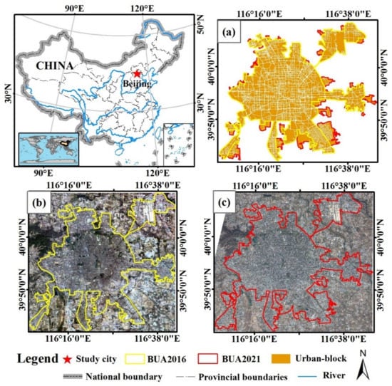
Figure 1.
The study area comprises (a) the BUA of Beijing in 2016 and 2021; (b) the BUA of Beijing in 2016; and (c) the BUA of Beijing in 2021. GaoFen-1 shows the true color composite of the blue, green, and red bands of the original image data.
In this study, we selected images of the Beijing area acquired by GF-1, including four images obtained in 2016 and two images obtained in 2021, and acquired data from https://data.cresda.cn/#/mapSearch (accessed on 26 January 2022). To avoid the influence on the land-cover classification results and dynamic analysis due to the seasonal differences between the two phases of data and image quality factors, such as cloudiness and exposure, the data were selected by data screening for both April and May in this study. The specific details are shown in Table 1. The GF-1 satellite is equipped with two 60 km-wide high-spatial-resolution sensor cameras (GF-1/PMS1 and GF-1/PMS2). The data collected by the panchromatic and multispectral sensors (PMSs) on GF-1 include panchromatic bands with a spatial resolution of 2 m and multispectral bands (blue, green, red, and near-infrared bands) with a spatial resolution of 8 m [25].

Table 1.
GF-1 data applied in this study.
The reference data used in this study were the boundary data of the BUA and the OpenStreetMap (OSM) data used to construct the city blocks.
- (1)
- The boundaries of the BUA were updated to 2016 and 2021 by applying GF-1 HRRS imagery and visual interpretation results based on the National Land Cover Dataset of China, which was produced by the Institute of the Chinese Academy of Sciences (http://www.resdc.cn/Datalist1.aspx?FieldTyepID=1,3 (accessed on 10 February 2022)). The average accuracy was greater than 95%, based on the 2016 and 2021 BUA statistical results provided by the National Bureau of Statistics of China (http://www.stats.gov.cn/tjsj/tjgb/ndtjgb/ (accessed on 10 February 2022)).
- (2)
- The OSM data were downloaded from the OpenStreetMap Foundation (http://www.openstreetmap.org/ (accessed on 28 January 2022)). The primary and secondary roads were mainly selected to construct the urban neighborhood units.
3. Methodology
Based on HRRS imagery supplemented with multi-source spatial information, in this study, a multi-level urban landscape pattern framework (urban administrative boundary, urban built-up area, urban block, and inner city land-cover objects) was developed. In addition, a multi-scale joint landscape pattern approach for multi-scale landscape pattern dynamic analysis of cities was constructed based on the high-precision urban land-cover mapping results for the two periods. The key steps in this study were (1) GF-1 data pre-processing, (2) high-precision spatiotemporal mapping of inner-city land cover, and (3) multi-scale joint landscape pattern dynamic analysis of the city (Figure 2).
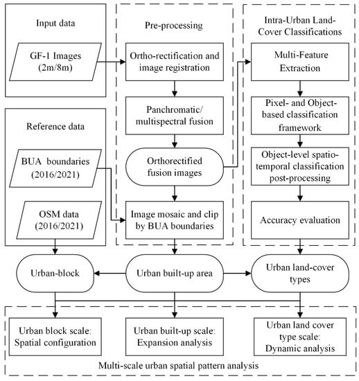
Figure 2.
Workflow of the procedure of the proposed urban multi-scale landscape pattern monitoring method.
3.1. Pre-processing of GF-1 Data
To ensure the spatial positioning accuracy and to further improve the spatial resolution, the GF-1 image data were preprocessed, including ortho-rectification, panchromatic/multispectral data fusion, and image mosaicking and clipping, using ENVI 5.0 commercial software. In this study, the GF-1 images were ortho-rectified based on the rational polynomial coefficient (RPC) model (using the RPC file in the system) [47] and were fused using the Gram–Schmidt pan-sharpening (GS) method [48]. Compared with fusion algorithms, such as Intensity Hus Saturation (IHS) transformation, Brovey transform, and Principal Component Analysis (PCA) transformation, the GS method improves the problem of the over-concentration of information in PCA and can preserve spatial texture information better without the band limitation; therefore, it has been more widely used in HRRS images [49]. Based on the above processing process, GF-1 ortho-rectification remote sensing images with a spatial resolution of 2 m were obtained. Based on the polynomial model [50], the GF-1 data for 2016 were geometrically corrected using ground control points collected from the 2021 GF-1 images, with an average root mean square error of <0.4 pixels, thus ensuring the relative positioning accuracy between the two phases of data. In addition, to facilitate the application of Beijing BUA images in the analysis, the pre-processed GF-1 images of 2016 and 2021 were mosaicked and clipped based on the corresponding BUA boundary data, respectively, thus obtaining the Beijing BUA images for the two periods (Figure 1b,c).
3.2. In-urban Land-cover Spatiotemporal Mapping
The land-cover changes were studied by obtaining multi-period land-cover results after performing land-cover classification. The post-classification comparison method is widely used because it can effectively reduce the error problem caused by atmospheric and environmental differences between multi-period images. The advantage of this method is that it can show land cover type changes and provide from–to type change information. However, the post-classification comparison method has the disadvantage of error accumulation, which makes it difficult to guarantee accuracy. Therefore, in this study, to ensure the accuracy of the multi-temporal land cover map of BUA, a complex land-cover classification chain was adopted, including multi-type feature extraction, a joint pixel–object classification framework, and object-level spatiotemporal classification post-processing based on expert knowledge.
3.2.1. Multi-Type Feature Extraction
In this section, we consider three types of feature sets (Table 2) to describe the inner-city land cover. Spectral indices and spatial features (e.g., morphology and texture) were used to reflect the physical attributes and spatial structural attributes of urban land-cover types, respectively. In addition, composite features were used to enhance the separability of the integrated feature types (e.g., urban buildings and urban surface water) in complex urban contexts.
Table 2.
Multiple features considered in this study.
- (1)
- Spectral index: The remote sensing spectral features can reflect the physical attributes of land-cover types and can visually portray land-cover type information. Spectral indices, such as the normalized difference vegetation index (NDVI) and the normalized difference water body index (NDWI), are indices constructed from spectral information in remote sensing images that better reflect the information about natural land surface attributes, such as water bodies, vegetation, and bare land in the spectral dimension [51,52]. Therefore, the NDWI/NDVI was used in this study to enhance the information about the water bodies, vegetation, and bare land in the inner city.
- (2)
- Spatial features: In HRRS images, the spatial features provide rich spatial information about the feature types, such as the geometry, texture, and morphological information, which can solve the confounding problem caused by relying only on spectral information [53]. Among them, the texture and morphological information are of greater concern and have been applied by scholars. They play an important role in the classification of features in HRRS images [54]. Therefore, in this study, the texture and morphological features were selected as the spatial features.
- (3)
- Composite features: Urban surface information has a certain degree of comprehensiveness and complexity due to features such as urban buildings and urban surface water [55,56]. To be able to enhance the extraction accuracy of urban surface information, many scholars have incorporated spatial features, such as the multi-scale angle, scale, and morphology of different urban feature types based on spectral features, thus forming composite features to enhance the separability of the urban surface information [57,58]. Therefore, in this study, the morphological building index (MBI) was used to enhance the urban buildings, the morphological shadow index (MSI) was used to enhance the shadow types, and the morphological large/small area water index (MLWI/MSWI) was used to enhance the information on urban surface water types.
3.2.2. A Pixel- and Object-Based Classification Framework
In this study, we adopted a joint pixel–object-based classification framework for land-cover mapping to resolve the uncertainty of the results brought about by using only a single classification method, thus improving the accuracy of land-cover mapping and the reliability of the multi-period land-cover classification results [65]. The pixel-based classification method can give full play to the significance of the spectral index features described in Section 3.2.1 for the spectral attributes of water bodies, vegetation, bare land, impervious surfaces, and other types, and can enhance the differentiability of the urban land surface types in the spectral dimension. The object-based classification method can fully utilize the spatial features described in Section 3.2.1 to increase the separability of the different types of features, such as buildings and roads. In addition, object-level mapping can avoid the problem of pretzel noise caused by pixel-based classification, and it can also unify them to the same scale for subsequent decision-level fusion processing. In the classification model used in this study, the random forest (RF) algorithm was used as the classification model because it is characterized by overfitting prevention, high stability, and strong generalization ability, and it can automatically perform feature selection among high-dimensional features [66]. Finally, the two strategies were fused at the decision level at the object-level scale, and land-cover mapping results with a higher accuracy were obtained through an iterative method of continuous optimization.
The steps of the joint pixel–object-based land-cover classification method are as follows: (1) Stack the multi-source features extracted in Section 3.2.1 to obtain a stacked feature F. (2) Use a multi-scale segmentation method to obtain an image segmentation object O. (3) Use an RF model to classify F and obtain the pixel-based classification results, pixel-based class map (pixel). (4) Use the pixel-based classification result R (pixel) and maximum voting for each segmentation object O to obtain the classification result, class map (PO). (5) Use the RF model to classify segmentation object O using feature F to obtain the object-based classification result, class-map (O). (6) Perform consistency judgment of class-map (PO) and class-map (O). When the classification result is consistent, obtain the initial class-map result. When the judgment result is inconsistent, repeat steps (3–6) for iterative computation until the process is terminated when the consistency judgment result is unchanged. (7) Obtain the final inconsistent segmentation object O using the maximum voting method for all of the results of the iterative computation in step (6) to obtain the maximum probability of the class, thus confirming the final type and finally obtaining the initial class-map results. In this study, the parameters of the random forest model were obtained by the trial-and-error method, i.e., the overall number of trees was 100 and the depth of each tree was 10. The details are shown in Figure 3.
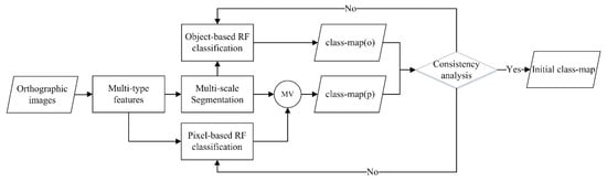
Figure 3.
Flowchart of a pixel- and object-based framework for intra-city land-cover classification.
3.2.3. Expert Knowledge-Based Post-Processing for Object-Level Spatiotemporal Classification
To ensure the accuracy of the spatiotemporal mapping of the internal urban land cover, in this study, expert knowledge-based object-level spatiotemporal classification post-processing rules were used to further check and refine the initial classification results. In this study, Table 3 was used to check the results of the unreasonable land cover objects between two phases of features based on the spatial correlation or interrelationship between the feature types. Based on this, a multi-temporal joint expert knowledge correction method was constructed to further automatically correct the unreasonable object results and obtain the final land-cover classification results. The advantage of this method is that it takes into account the spatial correlations between the features in the two periods and combines the spatial knowledge of the multi-temporal phases to correct the unreasonable object types, thus reducing the problem of the uncertainty of the feature types introduced in the post-processing phase based only on a single time.
Table 3.
Post-processing of classification based on spatiotemporal expert knowledge.
The steps were as follows: (1) To ensure that the images of different moments were analyzed at the same scale, the initial land-cover classification result for moment TA was segmented according to the initial land-cover classification result for moment T, and the initial land-cover classification result for moment TA with the same object boundary as moment T was obtained. (2) The unreasonable objects for moments T and TA were detected according to the rule set. (3) The unreasonable objects were automatically corrected according to the formula in Table 3 to obtain the results.
3.3. Accuracy Evaluation
In this study, internal urban land-cover mapping was generated in each computational step. The accuracy of the results was verified qualitatively through visual interpretation and quantitatively by a statistical confusion matrix containing the overall accuracy (OA), kappa coefficient (Kappa), producer’s accuracy (PA), and user’s accuracy (UA) [67]:
where TP, FN, FP, and TN are the areas of correct extraction, undetected water bodies, incorrect extraction, and non-water bodies that were correctly rejected, respectively; and T is the total area of the study area.
3.4. Analysis of Quantitative Changes in Multi-Scale Urban Landscape Patterns
To overcome the limitations caused by single-scale urban dynamic analysis, four levels of association were considered in our multi-level dynamic analysis study (Figure 4): intra-urban land-cover types, urban blocks, BUA, and urban administrative scales. First, using the information about the BUA boundary and inner urban land-cover types obtained from the HRRS images, we analyzed the urban expansion through the multi-scale union of the urban administrative boundary, BUA, and inner urban land-cover object layers (buildings, roads, and ISA types). Second, we obtained the fine-grained changes within the BUA by calculating the trajectories of land-cover types within the BUA. Finally, a joint landscape pattern analysis of the urban block and land-cover-type scales was conducted, focusing on the changes in the building and vegetation coverage and the configuration (landscape configuration indicators) that constitutes the urban-block scale.
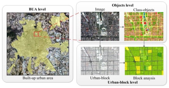
Figure 4.
Framework for the quantitative analysis of multi-scale urban landscape patterns.
3.4.1. Multi-scale Driven Analysis of BUA Levels
In this section, we use a method that combines the urban administrative area (UA), built-up urban area (BUA), and all-urban impervious surface area (AISA) to construct a multi-level combined BUA expansion evaluation index to analyze the urban expansion. Among them, the AISA is the artificial surface within the city, which specifically includes the sum of three types of feature information, i.e., buildings, roads, and ISA, in the urban land cover. The specific structural relationship is shown in Figure 5. The AISA is the internal component of the BUA, while the BUA is the internal component of the UA. In addition, the ratio of the AISA to the BUA and the ratio of the BUA to the UA were calculated to obtain the multi-level joint BUA expansion evaluation index. The equations are as follows:
where BUA, AISA, and UA are the area of the built-up urban area, the area of the all-urban impervious surfaces, and the area of the urban area, respectively. BUR and ABR are the ratio of the BUA to the UA and the ratio of the AISA to the BUA, respectively. The value of the BUR reflects the level of external expansion of the urbanization process. A higher value indicates a higher level of external expansion of the urbanization process, and a lower value indicates a lower level of external expansion of the urbanization process. The value of ABR reflects the density of the internal urban development. A higher ABR value indicates a higher density of internal urban development, and a lower value indicates a lower density of internal urban development.
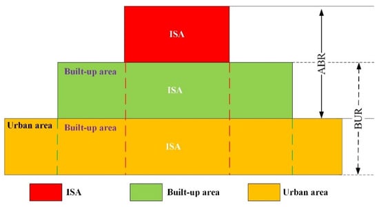
Figure 5.
Structural framework of the UA–BUA–AISA.
3.4.2. Analysis of in-Urban BUA Land-Cover Dynamics
Within the BUA of the city, the analysis was conducted from two perspectives: the proportion of the landscape components and the landscape pattern. In the landscape component analysis, the area of each landscape component and its percentage were quantified based on the spatial distribution of the landscape components to analyze the urban landscape characteristics [68]. Based on this, landscape pattern analysis was conducted at the patch scale. Among the many landscape pattern analysis methods, the landscape index is the most widely used index type. Landscape indices synthesize and generalize landscape information as quantitative composite indicators, which can be used to quantitatively evaluate the spatial combination, structure, and configuration of the landscape pattern and other characteristics.
In this study, the patch density (PD), maximum patch index (LPI), landscape shape index (LSI), aggregation index (AI), sprawl index (CONTAG), and Shannon diversity index (SHDI) were used to quantify the landscape pattern of the city and to analyze the changes in the landscape pattern of the study area based on the relevance of previous research. The concepts, calculation methods, thresholds, and ecological significance of these indices were described in previous studies. The FRAGSTATS 4.2.1 software was used to extract the landscape indices (Table 4).
Table 4.
Detailed information about the landscape indices implemented in FRAGSTATS 4.2.1 [69].
3.4.3. Dynamic Analysis of Urban Block-Level Landscape Patterns
In this study, inner-city land-cover analysis was conducted based on primary and secondary roads from OpenStreetMap (OSM) to construct the BUA block results. Among them, the building coverage ratio (BCR) and vegetation fraction (VF) are the two main landscape composition parameter values that have been studied and received attention. Namely, the BCR (VF) of each block is the ratio of the area covered by buildings (vegetation) to the total area. Thus far, fewer studies have focused on the variations in the building density and vegetation ratio at the urban block scale. Therefore, in this study, the BCR and VF at the urban block scale were constructed to dynamically evaluate and analyze the degree of human activity aggregation and vegetation greenness in the block patches. The BCR and VF were calculated as follows:
where is the ith block base; A is the area; is the area of the ith block base; and are the jth buildings and vegetation types of the ith block base, respectively; d is the density; and and are the building coverage and vegetation proportion of the ith block base, respectively. Based on this, the BCR and VF were counted in 0.2 steps in the interval of 0–1 and are divided into the following intervals for quantitative analysis: [0, 0.2], [0.2, 0.4], [0.4, 0.6], [0.6, 0.8], and [0.8, 1.0].
4. Results and Analysis
4.1. Urban Land-Cover Accuracy Validation
Accuracy assessment of the newly developed 2 m urban land-cover product was performed using a randomly selected sample (pixels). A total of 4000 samples were randomly collected in both 2016 and 2021, resulting in a total of 8000 randomly and equally distributed samples. As the area of urban land-cover types differed from year to year, stratified random sampling was used in this study to randomly select samples of land-cover types within cities during the different periods. We ensured the accuracy of the sample points through manual interpretation and field validation. The OA, Kappa, PA, and UA were used to conduct the accuracy evaluation [70].
As shown in Table 5, the overall accuracies of the land-cover classifications in 2016 and 2021 for the BUA of Beijing were 91.9% and 90.4%, respectively, and the kappa coefficients were 0.90 and 0.88, respectively. The overall accuracy of the land-cover results for the BUA in Beijing in both periods exceeded 90%, and the kappa coefficients were greater than 0.88, indicating the validity and stability of the classification method developed in this study. The validity and stability of the classification method developed in this study were demonstrated. Except for the impervious surface type, the mapping accuracy and user accuracy of the land-cover results of the remaining categories in 2016 and 2021 were greater than 86%, indicating that the misclassification and omission rates of the classification results were low. In summary, the land-cover classification framework for the BUA developed in this study can ensure the accuracy of the urban land-cover classification. Its overall accuracy was maintained at >90%, which meets the overall requirements of mapping and analysis.
Table 5.
Confusion matrix for Beijing land-cover mapping in 2016 and 2021 (UA—user’s accuracy; PA—producer’s accuracy).
4.2. Multi-scale Spatial Analysis of Urban Expansion
The results obtained in this study are presented in Table 6. The area of the BUA increased from 1312.2 km2 to 1460.3 km2, an increase of 148.1 km2. The BUR increased from 8.0% to 8.9%, an increase of 0.9%. In addition, the AISA increased from 718.3 km2 in 2016 to 868.1 km2 in 2021, an increase of 149.8 km2. The ABR increased from 54.7% to 59.4%, an increase of 4.7%. These results indicate that Beijing’s urbanization process was in rapid development within the city and the outward urban expansion was dramatic.
Table 6.
Area values from UA–BUA–AISA.
4.3. Analysis of Land-Cover Dynamics within Object-Level Cities
Figure 6 and Figure 7 show the statuses of the land cover within the BUA of Beijing in 2016 and 2021, respectively. Although the outward expansion of the BUA was significant, the roads and water bodies did not significantly change in terms of the overall patterns of their spatial distributions, indicating that the urban corridor landscape (road and water body elements) was relatively stable. During the period of 2016–2021, there was a significant increase in the areas of buildings and bare land patches, indicating that the BUA still had a high level of urbanization. In contrast, the areas of vegetation and the ISA significantly decreased during this period, indicating that the accelerated urbanization process compressed the vegetation and ISA.
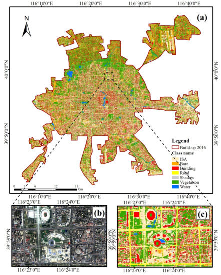
Figure 6.
(a) Land-cover mapping of the BUA in Beijing in 2016; (b) detailed comparison of GaoFen-1 imagery; and (c) classification results.
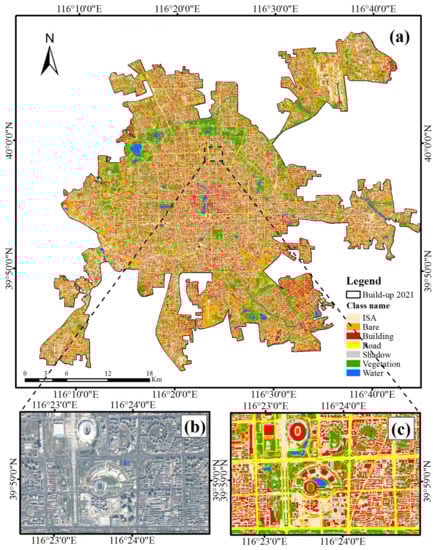
Figure 7.
(a) Land-cover mapping of the BUA in Beijing in 2021; (b) detailed comparison of GaoFen-1 imagery; and (c) classification results.
As can be seen from Table 7, the areas of the water bodies, roads, and ISA increased from 17.8 km2, 45.8 km2, and 372.2 km2 in 2016 to 24 km2, 53.2 km2, and 374.3 km2 in 2021, with increases of 6.3 km2, 7.4 km2, and 2.1 km2, respectively. Their proportions increased from 1.4%, 3.5%, and 28.4% in 2016 to 1.6%, 3.6%, and 25.6% in 2021, with increases of 0.2%, 0.1%, and −2.8%, respectively, indicating the stability of the urban corridor pattern. The areas of the buildings and bare land increased from 231.6 km2 and 171.4 km2 to 271.6 km2 and 327.7 km2, with increases of 39.9 km2 and 156.3 km2, respectively; and their proportions increased from 17.7% and 13.1% to 18.6% and 22.4%, with increases of 0.9% and 9.3%, respectively, indicating that the urbanization process remained at a significant level. In contrast, the area of vegetation decreased from 404.8 km2 to 240.4 km2, a decrease of 164.4 km2, and its proportion decreased from 30.8% to 16.5%, a decrease of 14.3%, indicating that the urbanization process occupied the previously vegetated areas, to some extent.
Table 7.
Dynamic changes in the urban land cover types between 2016 and 2021.
Figure 8 shows the landscape pattern indices of the BUA in Beijing between 2016 and 2021. In particular, Figure 8a assesses all land-cover types as a whole at the landscape level, and Figure 8b–f evaluate the landscape pattern index for each land-cover type at the patch level. The landscape pattern indices used in the analysis were defined in Section 3.4.2.
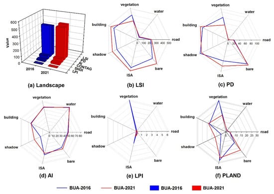
Figure 8.
Landscape indices of the BUA in Beijing between 2016 and 2021. (a) Values of LPI, SHDI, CONTAG, AI, PD, and LSI for the landscape scale indicator; (b–f) represent the values of LSI, PD, AI, LPI, and PLAND, respectively, for the class scale indicator.
The LPI decreased from 6.2 to 1.0, with the largest patch decreasing by 5.2, reflecting an overall increase in the utilization of development within the BUA in Beijing. The LSI and SHDI increased from 455.4 and 1.6 in 2016 to 508.9 and 1.7 in 2021, with increases of 53.5 and 0.1, respectively, indicating that the diversity of the landscape types in Beijing increased during these 5 years. The CONTAG and AI increased from 25.9 and 57.4 to 30.7 and 55.5, with increases of 4.8 and 3.3, respectively, indicating that the connectivity and aggregation of the patches increased further; thus, the land use in the BUA in Beijing increased the connectivity of the land types during these 5 years. The development and utilization of the BUA in Beijing increased the connectivity and aggregation of the land types. The AI of the bare land increased from 50.2 to 54.7, an increase of 4.5, which was the most significant increase among all of the types, indicating that there were fewer major changes within the original BUA, and the significant changes were brought about by the expansion of the BUA.
4.4. Multi-Scale Joint Analysis at the City Block Level
As can be seen from Figure 9, in the outward expansion area of the BUA from 2016 to 2021, the block building density was higher in the northwest and southeast areas of the BUA, and it had a certain scale initially. However, the overall block building density in the outward expansion area of the BUA remained in the early stage of construction during these 5 years. Within the part of the BUA that remained unchanged during the 5 years, the urban center did not change much, and the increase in the block building density was more significant in the periphery of the adjacent urban center. The overall building density increased steadily with fewer peaks, indicating that Beijing, which had a high level of urbanization, was still in the process of rapid and stable urbanization during the period of 2016–2021. As shown in Figure 10, the overall vegetation density decreased at the block scale, while the vegetation density remained high in the northern part of the BUA. This indicates that the accelerated urbanization process had a certain impact on the urban greening in the city center and adjacent areas, while it had less of an impact on the northern part of the BUA, maintaining a high greening rate at the block scale.
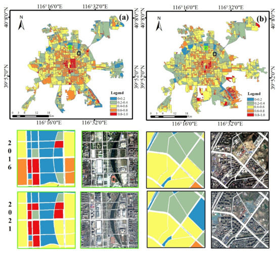
Figure 9.
(a,b) show the results of the building coverage ratio in Beijing in 2016 and 2021, respectively. Note: the green and black boxes represent the detailed comparison results of the building coverage ratio and GaoFen-1 images for the two regions during 2016–2021.
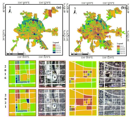
Figure 10.
(a,b) show the results of the vegetation fraction in Beijing in 2016 and 2021, respectively. Note: the red and yellow boxes represent the detailed comparison results of the vegetation fraction and GaoFen-1 images for the two regions during 2016–2021.
As can be seen fromFigure 11a,b, the significant increases in the BCR were mainly concentrated within the intervals [0.2, 0.4] and [0.4, 0.6], the significant decreases were in the interval [0, 0.2], and there were no significant changes in the other intervals. The number of blocks within intervals [0.2, 0.4] and [0.4, 0.6] increased from 364 and 594 in 2016 to 454 and 801 in 2021, with increases of 90 and 347, respectively, and their percentages increased from 11.7% and 19.1% to 13.6% and 23.9%, with increases of 1.9% and 4.8%, respectively, exhibiting a general trend of increasing building coverage, thus reflecting the continued gradual increase in the urbanization process. Within interval [0,0.2], the number of blocks decreased from 1458 in 2016 to 1377 in 2021, a decrease of 81, and the percentage decreased from 47% to 41.1%, a decrease of 5.9%, with some undeveloped and underutilized plots or low-developed plots undergoing gradual development and utilization. In summary, it can be concluded that the urban area of Beijing City experienced steady urbanization and a stage of increasing utilization from 2016 to 2021.
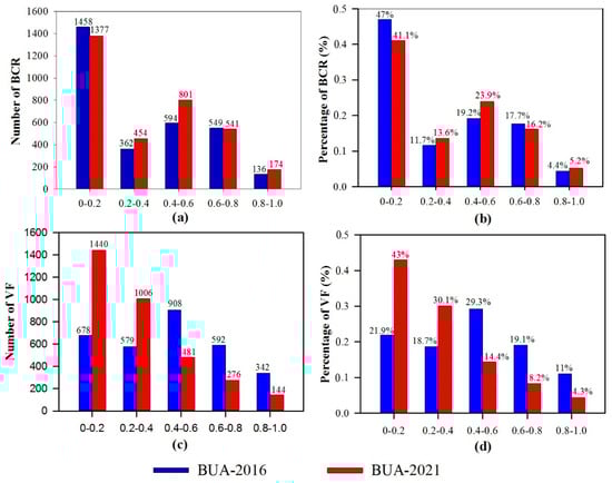
Figure 11.
Statistical analysis of the building coverage ratio (BCR) and vegetation fraction (VF) within the city-block scale of urban built-up areas: (a,b) indicate the number and proportion of the BCR within the statistical interval, respectively; (c,d) indicate the number and proportion of the VF within the statistical interval, respectively.
As can be seen from Figure 11c,d, the number of blocks with VF in intervals [0, 0.2] and [0.2, 0.4] increased from 678 and 579 in 2016 to 1440 and 1006 in 2021, with increases of 762 and 427, respectively, and their percentages increased from 21.9% and 18.7% to 43% and 30.1%, with increases of 21.1% and 11.4%, respectively. Meanwhile, the number of VFs in intervals [0.4,0.6], [0.6,0.8], and [0.8,1.0] decreased from 908, 592, and 342 to 481, 276, and 144, with decreases of 566, 316, and 198, and their percentages decreased from 29.3%, 19.1%, and 11% to 14.4%, 8.2%, and 4.3%, with decreases of 14.9%, 10.9%, and 6.7%, respectively. The significant increase in interval [0, 0.4] and the significant decrease in interval [0.4, 1] reflect the increase in VF as contiguous vegetation blocks were exploited. This also reflects the direct change in and occupation of the urban greenspace landscape pattern due to the increase in urbanization processes from 2016 to 2021.
5. Discussion
5.1. Comparison and Analysis of the Accuracy of Urban Land-Cover Mapping
In this section, the classification accuracy, applied methods, and important sources of errors are discussed. First, the land-cover classification results are consistent with the area of the visual interpretation and validation data results. Therefore, the remote sensing classification method proposed is credible in this study area. In the classification and dynamic analysis of urban land-cover at the scale of a BUA, medium-resolution remote sensing images are still more widely used. Compared with medium-resolution remote sensing images used for the land-cover classification mapping of BUA [71,72], the overall accuracy of the method developed in this study is higher (1.0–2.0% higher), the land-cover types are richer, and the spatial patterns of the different types of land-cover are portrayed better. For example, HRRS images can reflect the different spatial patterns of buildings, such as single buildings, continuous buildings, and large factory buildings. It can be concluded that the land-cover mapping results based on HRRS images are more reasonable for constructing a multi-scale analysis framework that includes rich object types, urban blocks, and BUAs. At present, most of the studies on HRRS image land-cover mapping focus on method testing or dynamic analysis of local typical urban areas [73], but the classification method constructed in this study for BUA land-cover and dynamic analyses was applied to the complete BUA in two time periods, indicating that this study has a certain degree of application demonstration value and reference significance. In addition, in terms of accuracy, although the classification accuracy was similar to that of other typical urban areas (within 2.0%) [74,75], the larger the selected study area is, the more complex the land-cover type characteristics reflected in the HRRS images are, according to the comprehensive and complex characteristics of cities. Therefore, the classification accuracy can be maintained under more complex application scenarios, further indicating the effectiveness of this research method.
There are two reasons for the decrease in accuracy. The first reason is the insufficient spectral information. Although spatial features, such as the morphology and texture, and comprehensive indices were used to supplement the spectral features in this study to improve the overall classification accuracy, the complexity of the scenes and the diversity of the surface types in Beijing, a mega-city in China, made the same object with different spectra or different objects with the same spectrum phenomena more notable. Thus, supplementary spatial information cannot completely replace spectral information, which affects the classification accuracy. The second reason is that, to ensure the classification accuracy and avoid the influence of noise in the incoming bands, such as clouds and fog, some of the selected image time phases were not in the vegetation growing season, which led to lower extraction results for some vegetation. However, because spatial information was used to enhance the vegetation, the confusion between vegetation and bare land was greatly reduced. In addition, the high accuracy of the extraction results of the buildings and shadows also indirectly reflected the correct trend of the reduction in the vegetation types. Therefore, for HRRS images, the non-growing-season images will cause a certain degree of error in the extraction of the vegetation type information, but this will not cause a notable effect.
5.2. Comparison and Analysis of the Effects of Urban Landscape Patterns
The results of this study were consistent with the general trend of the results of the analysis of urban landscape patterns at a single scale (e.g., BUA, urban type scale, and city block scale) in the current study [76,77,78], indicating the validity of this study’s analysis. Among them, in terms of urban expansion, compared with other similar studies [79,80], the joint multi-scale evaluation method constructed by this study’s methodology can quantitatively describe the external expansion of cities while also depicting the internal expansion of cities, thus reflecting the degree of urbanization more accurately. In particular, for cities whose external expansion is gradually stabilizing while their internal expansion is still on the rise, this research method can more accurately reflect the urbanization process of such cities than that when relying on a single external expansion evaluation index. In addition, the BUA is widely studied and applied as a complete urban ecosystem unit. Compared with most studies that use medium-resolution remote sensing images to obtain complete information regarding the extent of BUAs and their internal land cover [81,82], the urban landscape pattern evaluation indexes constructed based on HRRS images in this study can provide high-dimensional and more comprehensive characteristics of urban sprawl and internal spatial patterns, further reflecting their rationality and necessity. In analyzing the spatial pattern characteristics within the city, the multi-scale composite index constructed in this study, based on refined land-cover mapping and using city blocks as the landscape analysis unit, is less likely to segment the spatial characteristics of the landscape pattern and is able to present the ecological functional characteristics of the city more comprehensively than the regular grid [38] or city block scales [83] used in previous studies.
The impact of this study on the landscape pattern analysis method is mainly focused on two aspects: On one hand, it is focused on the construction of landscape pattern evaluation units. Although this study adopted the city blocks constructed by the modified urban road network data to express the urbanization process and the evaluation units were more reasonable, the lack of unified standards for the construction of city block units for remote sensing applications caused the results of landscape pattern analysis under different evaluation units to fluctuate, to a certain extent. On the other hand, it is focused on the limitations of landscape pattern evaluation indexes. Although the refined statistics of land-cover types, the construction of typical landscape pattern analysis indicators, and the expansion of multi-scale joint analysis methods in this study can effectively express the landscape pattern characteristics of cities, the comprehensive and complex nature of cities makes it difficult for the current indicators to fully and comprehensively portray the urban landscape pattern, thus leading to a certain degree of variation in the studies of different scholars, but, in general, the trends were generally consistent and did not have a significant impact on the final analysis.
5.3. Limitations and Prospects of the Study
The advantage of the classification method developed in this study is that the automatic mapping of land cover was satisfactorily achieved by combining multi-source features according to the characteristics of different urban land-cover types and using the object–pixel–spatiotemporal expert knowledge method. The shortcoming of this method is that the insufficient spectral information from HRRS images leads to inevitable mixing and omission problems, which make the classification results less accurate. Therefore, in subsequent research, we will try to introduce data sources with the advantages of spectral or temporal dimensions and will construct a multi-source data fusion extraction method to further improve the accuracy of urban land-cover classification. In addition, in this study, the update of BUA boundaries was performed by the manual interpretation of HRRS data, which can guarantee accuracy but is also more time-consuming. In contrast, the current study on the application of night-light data was able to identify the BUA boundaries better at a large scale. Therefore, we will further study the fusion method of night-light data and HRRS image data for developing an automatic extraction method of BUAs at a detailed scale.
In terms of urban landscape pattern analysis methods, the multi-scale joint landscape pattern analysis method constructed in this study can provide a comprehensive analysis of the external expansion, internal expansion, and internal spatial pattern characteristics of a city, but due to the limitation of the data sources of high-definition remote sensing images, the current studies have all been focused on horizontal dimensional expansion and have not yet involved the study of the vertical dimension of cities. At present, with the development of satellite technology, there have been research advances in urban building height [84,85] or vegetation height monitoring [86,87]. Therefore, in the subsequent research, we will further try to combine satellite data with altimetry capability loads to obtain refined land-cover height information and be able to further construct 3D urban landscape pattern evaluation indexes, such as the volume, density, and volume ratio, to deeply characterize the urban landscape pattern from higher dimensions.
6. Conclusions
The focus of this study was to make full use of multi-period HRRS images to extract land-cover information for BUAs and their internal areas. Based on this, we constructed a framework for multi-scale joint analysis and evaluation methods, such as urban administrative district–BUA–urban block–land type elements to achieve the joint macro–micro dynamic change analysis and evaluation of cities. In this study, we took Beijing, the capital of China and also a mega-city in China, as an example to test and verify the effectiveness of the newly developed method. The main conclusions of this study are as follows.
- (1)
- From the perspective of multi-temporal urban land-cover mapping, the spatiotemporal extraction method for intra-city land cover developed in this study can ensure the accuracy of the multi-period land-cover extraction results. Therefore, it provides a guarantee for the analysis of multi-temporal urban spatial pattern changes.
- (2)
- The joint multi-scale urban spatial pattern dynamic analysis method developed in this study can better overcome the analytical limitations caused by the use of single-scale evaluation methods. In terms of analyzing the expansion of BUAs, the joint analysis method of the object–BUA–urban administrative area layer developed in this study can jointly analyze the expansion of BUAs from the two levels of their external expansion and internal expansion in a refined way, overcoming the problem of a single data source only expressing the expansion of BUA. In addition, a multi-level joint analysis method of BUA–block–object was constructed within the BUA to analyze the spatial patterns of and changes in land-cover types within the city, which makes up for the problem that a single scale can only reflect the change trajectory of land-cover types.
- (3)
- We found that 2 m-resolution remote sensing images, whether used in the high-precision and high-resolution land-cover results provided or in the evaluation method developed in this study, were applicable. However, when 30 m Landsat data were applied for this purpose, it was difficult to guarantee the evaluation effect, such as the spatial information provided, due to the resolution.
Author Contributions
Conceptualization, Z.L. and X.Y.; methodology, Z.L.; software, Z.L.; validation, Z.L. and Y.L.; formal analysis, Z.L.; investigation, Z.L.; resources, Z.L. and X.Y.; data curation, Z.L.; writing—original draft preparation, Z.L.; writing—review and editing, Z.L. and X.Y.; visualization, Z.L.; supervision, X.Y.; funding acquisition, Z.L. and X.Y. All authors have read and agreed to the published version of the manuscript.
Funding
This research was funded by the National Natural Science Foundation of China (Grant No. 42101383).
Data Availability Statement
GF-1 data used in this study are available for download from the China Center for Resources Satellite Data and Application at https://data.cresda.cn/#/mapSearch (accessed on 26 January 2022). the National Land Cover Dataset of China can be accessed at http://www.resdc.cn/Datalist1.aspx?FieldTyepID=1,3 (accessed on 10 February 2022)). the 2016 and 2021 BUA statistical results are available at http://www.stats.gov.cn/tjsj/tjgb/ndtjgb/ (accessed on 10 February 2022). The OSM data are downloaded from the OpenStreetMap Foundation (http://www.openstreetmap.org/ (accessed on 28 January 2022)). All the data presented in this study are available on request from the corresponding author.
Conflicts of Interest
The authors declare no conflict of interest.
References
- Chen, Y.; Liu, Z.; Zhou, B.B. Population-environment dynamics across world’s top 100 urban agglomerations: With implications for transitioning toward global urban sustainability. J. Environ. Manag. 2022, 319, 115630. [Google Scholar] [CrossRef] [PubMed]
- Jiang, H.; Guo, H.; Sun, Z.; Xing, Q.; Zhang, H.; Ma, Y.; Li, S. Projections of urban built-up area expansion and urbanization sustainability in China’s cities through 2030. J. Clean. Prod. 2022, 367, 133086. [Google Scholar] [CrossRef]
- Zhang, X.; Han, L.; Wei, H.; Tan, X.; Zhou, W.; Li, W.; Qian, Y. Linking urbanization and air quality together: A review and a perspective on the future sustainable urban development. J. Clean. Prod. 2022, 346, 130988. [Google Scholar] [CrossRef]
- Qian, Y.; Chakraborty, T.C.; Li, J.; Li, D.; He, C.; Sarangi, C.; Leung, L.R. Urbanization impact on regional climate and extreme weather: Current understanding, uncertainties, and future research directions. Adv. Atmos. Sci. 2022, 39, 819–860. [Google Scholar] [CrossRef]
- Ahmed, Z.; Zafar, M.W.; Ali, S. Linking urbanization, human capita, and the ecological footprint in G7 countries: An empirical analysis. Sustain. Cities Soc. 2020, 55, 102064. [Google Scholar] [CrossRef]
- Zhou, D.; Tian, Y.; Jiang, G. Spatio-temporal investigation of the interactive relationship between urbanization and ecosystem services: Case study of the Jingjinji urban agglomeration, China. Ecol. Indic. 2018, 95, 152–164. [Google Scholar] [CrossRef]
- Uttara, S.; Bhuvandas, N.; Aggarwal, V. Impacts of urbanization on environment. Int. J. Res. Eng. Appl. Sci. 2012, 2, 1637–1645. [Google Scholar]
- Hou, B.; Nazroo, J.; Banks, J.; Marshall, A. Are cities good for health? A study of the impacts of planned urbanization in China. Int. J. Epidemiol. 2019, 48, 1083–1090. [Google Scholar] [CrossRef]
- Liang, L.; Wang, Z.; Li, J. The effect of urbanization on environmental pollution in rapidly developing urban agglomerations. J. Clean. Prod. 2019, 237, 117649. [Google Scholar] [CrossRef]
- Kuddus, M.A.; Tynan, E.; McBryde, E. Urbanization: A problem for the rich and the poor? Public Health Rev. 2020, 41, 1–4. [Google Scholar] [CrossRef]
- Dadashpoor, H.; Azizi, P.; Moghadasi, M. Land use change, urbanization, and change in landscape pattern in a metropolitan area. Sci. Total Environ. 2019, 655, 707–719. [Google Scholar] [CrossRef] [PubMed]
- Zhao, Q.; Wen, Z.; Chen, S.; Ding, S.; Zhang, M. Quantifying land use/land cover and landscape pattern changes and impacts on ecosystem services. Int. J. Environ. Res. Public Health 2020, 17, 126. [Google Scholar] [CrossRef] [PubMed]
- Drummond, M.A.; Stier, M.P.; Diffendorfer, J.J.E. Historical land use and land cover for assessing the northern Colorado Front Range urban landscape. J. Maps 2019, 15, 89–93. [Google Scholar] [CrossRef]
- Chi, Y.; Zhang, Z.; Gao, J.; Xie, Z.; Zhao, M.; Wang, E. Evaluating landscape ecological sensitivity of an estuarine island based on landscape pattern across temporal and spatial scales. Ecol. Indic. 2019, 101, 221–237. [Google Scholar] [CrossRef]
- Huang, L.; Wu, J.; Yan, L. Defining and measuring urban sustainability: A review of indicators. Landsc. Ecol. 2015, 30, 1175–1193. [Google Scholar] [CrossRef]
- Kadhim, N.; Mourshed, M.; Bray, M. Advances in remote sensing applications for urban sustainability. Euro-Mediterr. J. Environ. Integr. 2016, 1, 1–22. [Google Scholar] [CrossRef]
- Collins, J.; Dronova, I. Urban landscape change analysis using local climate zones and object-based classification in the Salt Lake Metro Region. Utah. USA. Remote Sens. 2019, 11, 1615. [Google Scholar] [CrossRef]
- Yu, B.; Shu, S.; Liu, H.; Song, W.; Wu, J.; Wang, L.; Chen, Z. Object-based spatial cluster analysis of urban landscape pattern using nighttime light satellite images: A case study of China. Int. J. Geogr. Inf. Sci. 2014, 28, 2328–2355. [Google Scholar] [CrossRef]
- Lin, Q.; Guo, J.; Yan, J.; Heng, W. Land use and landscape pattern changes of Weihai, China based on object-oriented SVM classification from Landsat MSS/TM/OLI images. European Journal of Remote Sensing. 2018, 51, 1036–1048. [Google Scholar] [CrossRef]
- Phiri, D.; Simwanda, M.; Salekin, S.; Nyirenda, V.R.; Murayama, Y.; Ranagalage, M. Sentinel-2 data for land cover/use mapping: A review. Remote Sens. 2020, 12, 2291. [Google Scholar] [CrossRef]
- Lamine, S.; Petropoulos, G.P.; Singh, S.K.; Szabó, S.; Bachari, N.E.I.; Srivastava, P.K.; Suman, S. Quantifying land use/land cover spatio-temporal landscape pattern dynamics from Hyperion using SVMs classifier and FRAGSTATS®. Geocarto Int. 2018, 33, 862–878. [Google Scholar] [CrossRef]
- Huang, X.; Wang, Y.; Li, J.; Chang, X.; Cao, Y.; Xie, J.; Gong, J. High-resolution urban land-cover mapping and landscape analysis of the 42 major cities in China using ZY-3 satellite images. Sci. Bull. 2020, 65, 1039–1048. [Google Scholar] [CrossRef]
- Tong, X.Y.; Xia, G.S.; Lu, Q.; Shen, H.; Li, S.; You, S.; Zhang, L. Land-cover classification with high-resolution remote sensing images using transferable deep models. Remote Sens. Environ. 2020, 237, 111322. [Google Scholar] [CrossRef]
- Toth, C.; Jóźków, G. Remote sensing platforms and sensors: A survey. ISPRS J. Photogramm. Remote. Sens. 2016, 115, 22–36. [Google Scholar] [CrossRef]
- Chen, L.; Letu, H.; Fan, M.; Shang, H.; Tao, J.; Wu, L.; Zhang, T. An Introduction to the Chinese High-Resolution Earth Observation System: Gaofen-1~ 7 Civilian Satellites. J. Remote. Sens. 2022, 2022, 9769536. [Google Scholar] [CrossRef]
- Zhong, B.; Yang, A.; Liu, Q.; Wu, S.; Shan, X.; Mu, X.; Hu, L.; Wu, J. Analysis Ready Data of the Chinese GaoFen Satellite Data. Remote Sens. 2021, 13, 1709. [Google Scholar] [CrossRef]
- Wang, J.; Bretz, M.; Dewan, M.A.A.; Delavar, M.A. Machine learning in modelling land-use and land cover-change (LULCC): Current status, challenges and prospects. Sci. Total Environ. 2022, 2022, 153559. [Google Scholar] [CrossRef]
- Zhang, H.; Shi, W.; Wang, Y.; Hao, M.; Miao, Z. Classification of very high spatial resolution imagery based on a new pixel shape feature set. IEEE Geosci. Remote. Sens. Lett. 2013, 11, 940–944. [Google Scholar] [CrossRef]
- Pesaresi, M.; Gerhardinger, A.; Kayitakire, F. A robust built-up area presence index by anisotropic rotation-invariant textural measure. IEEE J. Sel. Top. Appl. Earth Obs. Remote Sens. 2008, 1, 180–192. [Google Scholar] [CrossRef]
- Song, B.; Li, J.; Dalla Mura, M.; Li, P.; Plaza, A.; Bioucas-Dias, J.M.; Chanussot, J. Remotely sensed image classification using sparse representations of morphological attribute profiles. IEEE Trans. Geosci. Remote Sens. 2013, 52, 5122–5136. [Google Scholar] [CrossRef]
- Cavallaro, G.; Falco, N.; Dalla Mura, M.; Benediktsson, J.A. Automatic attribute profiles. IEEE Trans. Image Process. 2017, 26, 1859–1872. [Google Scholar] [CrossRef] [PubMed]
- Salehi, B.; Ming Zhong, Y.; Dey, V. A review of the effectiveness of spatial information used in urban land cover classification of VHR imagery. Int. J. Geoinf. 2012, 8, 35. [Google Scholar]
- Zhang, P.; Ke, Y.; Zhang, Z.; Wang, M.; Li, P.; Zhang, S. Urban land use and land cover classification using novel deep learning models based on high spatial resolution satellite imagery. Sensors 2018, 18, 3717. [Google Scholar] [CrossRef] [PubMed]
- Jozdani, S.E.; Johnson, B.A.; Chen, D. Comparing deep neural networks, ensemble classifiers, and support vector machine algorithms for object-based urban land use/land cover classification. Remote Sens. 2019, 11, 1713. [Google Scholar] [CrossRef]
- Chen, J.; Chen, J.; Liao, A.; Cao, X.; Chen, L.; Chen, X.; Mills, J. Global land cover mapping at 30 m resolution: A POK-based operational approach. ISPRS J. Photogramm. Remote Sens. 2015, 103, 7–27. [Google Scholar] [CrossRef]
- Lei, D.; Ran, G.; Zhang, L.; Li, W. A Spatiotemporal Fusion Method Based on Multiscale Feature Extraction and Spatial Channel Attention Mechanism. Remote Sens. 2022, 14, 461. [Google Scholar] [CrossRef]
- Jia, Y.; Tang, L.; Xu, M.; Yang, X. Landscape pattern indices for evaluating urban spatial morphology–A case study of Chinese cities. Ecol. Indic. 2019, 99, 27–37. [Google Scholar] [CrossRef]
- Li, Z.; Zhou, C.; Yang, X.; Chen, X.; Meng, F.; Lu, C.; Qi, W. Urban landscape extraction and analysis in the mega-city of China’s coastal regions using high-resolution satellite imagery: A case of Shanghai, China. Int. J. Appl. Earth Obs. Geoinf. 2018, 72, 140–150. [Google Scholar] [CrossRef]
- Yu, W.; Zhou, W.; Jing, C.; Zhang, Y.; Qian, Y. Quantifying highly dynamic urban landscapes: Integrating object-based image analysis with Landsat time series data. Landsc. Ecol. 2021, 36, 1845–1861. [Google Scholar] [CrossRef]
- Chen, D.; Zhang, F.; Jim, C.Y.; Bahtebay, J. Spatio-temporal evolution of landscape patterns in an oasis city. Environ. Sci. Pollut. Res. 2022, 1–15. [Google Scholar] [CrossRef]
- Li, H.; Peng, J.; Yanxu, L.; Yi’na, H. Urbanization impact on landscape patterns in Beijing City, China: A spatial heterogeneity perspective. Ecol. Indic. 2017, 82, 50–60. [Google Scholar] [CrossRef]
- Rendenieks, Z.; Tērauds, A.; Nikodemus, O.; Brūmelis, G. Comparison of input data with different spatial resolution in landscape pattern analysis–a case study from northern latvia. Appl. Geogr. 2017, 83, 100–106. [Google Scholar] [CrossRef]
- Huang, X.; Wen, D.; Li, J.; Qin, R. Multi-level monitoring of subtle urban changes for the megacities of China using high-resolution multi-view satellite imagery. Remote Sens. Environ. 2017, 196, 56–75. [Google Scholar] [CrossRef]
- Du, S.; Du, S.; Liu, B.; Zhang, X. Mapping large-scale and fine-grained urban functional zones from VHR images using a multi-scale semantic segmentation network and object based approach. Remote Sens. Environ. 2021, 261, 112480. [Google Scholar] [CrossRef]
- Tan, Y.; Xu, H.; Zhang, X. Sustainable urbanization in China: A comprehensive literature review. Cities 2016, 55, 82–93. [Google Scholar] [CrossRef]
- Myint, S.W.; Gober, P.; Brazel, A.; Grossman-Clarke, S.; Weng, Q. Per-pixel vs. object-based classification of urban land-cover extraction using high spatial resolution imagery. Remote Sens. Environ. 2011, 115, 1145–1161. [Google Scholar] [CrossRef]
- Liu, Q.; Yu, T.; Zhang, W. Validation of GaoFen-1 Satellite Geometric Products Based on Reference Data. J. Indian Soc. Remote Sens. 2019, 47, 1331–1346. [Google Scholar] [CrossRef]
- Wei, J.; Yang, H.; Tang, W.; Li, Q. Spatiotemporal-Spectral Fusion for Gaofen-1 Satellite Images. IEEE Geosci. Remote Sens. Lett. 2021, 19, 1–5. [Google Scholar] [CrossRef]
- Alimuddin, I.; Sumantyo, J.T.S.; Kuze, H. Assessment of pan-sharpening methods applied to image fusion of remotely sensed multi-band data. Int. J. Appl. Earth Obs. Geoinf. 2012, 18, 165–175. [Google Scholar]
- Wang, J.; Ge, Y.; Heuvelink, G.B.; Zhou, C.; Brus, D. Effect of the sampling design of ground control points on the geometric correction of remotely sensed imagery. Int. J. Appl. Earth Obs. Geoinf. 2012, 18, 91–100. [Google Scholar] [CrossRef]
- Feyisa, G.L.; Meilby, H.; Fensholt, R.; Proud, S.R. Automated Water Extraction Index: A new technique for surface water mapping using Landsat imagery. Remote Sens. Environ. 2014, 140, 23–35. [Google Scholar] [CrossRef]
- Hashim, H.; Abd Latif, Z.; Adnan, N.A. Urban vegetation classification with NDVI threshold value method with very high resolution (VHR) Pleiades imagery. The International Archives of Photogrammetry. Remote Sens. Spat. Inf. Sci. 2019, 42, 237–240. [Google Scholar]
- Pu, R.; Landry, S.; Yu, Q. Object-based urban detailed land-cover classification with high spatial resolution IKONOS imagery. Int. J. Remote Sens. 2011, 32, 3285–3308. [Google Scholar] [CrossRef]
- Lv, Z.; Liu, T.; Benediktsson, J.A.; Falco, N. Land cover change detection techniques: Very-high-resolution optical images: A review. IEEE Geosci. Remote Sens. Mag. 2021, 10, 44–63. [Google Scholar] [CrossRef]
- Huang, C.; Chen, Y.; Zhang, S.; Wu, J. Detecting, extracting, and monitoring surface water from space using optical sensors: A review. Rev. Geophys. 2018, 56, 333–360. [Google Scholar] [CrossRef]
- Li, J.; Huang, X.; Tu, L.; Zhang, T.; Wang, L. A review of building detection from very high resolution optical remote sensing images. GIScience Remote. Sens. 2022, 59, 1199–1225. [Google Scholar] [CrossRef]
- Duro, D.C.; Franklin, S.E.; Dubé, M.G. Multi-scale object-based image analysis and feature selection of multi-sensor earth observation imagery using random forests. Int. J. Remote Sens. 2012, 33, 4502–4526. [Google Scholar] [CrossRef]
- Bi, Q.; Qin, K.; Zhang, H.; Zhang, Y.; Li, Z.; Xu, K. A multi-scale filtering building index for building extraction in very high-resolution satellite imagery. Remote Sens. 2019, 11, 482. [Google Scholar] [CrossRef]
- Rouse, J.W., Jr.; Haas, R.H.; Deering, D.W.; Schell, J.A.; Harlan, J.C. Monitoring the Vernal Advancement and Retrogradation (Green Wave Effect) of Natural Vegetation; NASA/GSFC Type III Final Report; NASA/GSFC: Greenbelt, MD, USA, 1974. [Google Scholar]
- McFeeters, S.K. The use of the Normalized Difference Water Index (NDWI) in the delineation of open water features. Int. J. Remote Sens. 1996, 17, 1425–1432. [Google Scholar] [CrossRef]
- Huang, X.; Han, X.; Zhang, L.; Gong, J.; Liao, W.; Benediktsson, J.A. Generalized differential morphological profiles for remote sensing image classification. IEEE J. Sel. Top. Appl. Earth Obs. Remote Sens. 2016, 9, 1736–1751. [Google Scholar] [CrossRef]
- Ruiz Hernandez, I.E.; Shi, W. A Random Forests classification method for urban land-use mapping integrating spatial metrics and texture analysis. Int. J. Remote Sens. 2018, 39, 1175–1198. [Google Scholar] [CrossRef]
- Huang, X.; Zhang, L. Morphological building/shadow index for building extraction from high-resolution imagery over urban areas. IEEE J. Sel. Top. Appl. Earth Obs. Remote Sens. 2011, 5, 161–172. [Google Scholar] [CrossRef]
- Li, Z.; Yang, X. Fusion of high-and medium-resolution optical remote sensing imagery and GlobeLand30 products for the automated detection of intra-urban surface water. Remote Sens. 2020, 12, 4037. [Google Scholar] [CrossRef]
- Zhang, C.; Chen, Y.; Yang, X.; Gao, S.; Li, F.; Kong, A.; Sun, L. Improved remote sensing image classification based on multi-scale feature fusion. Remote Sens. 2020, 12, 213. [Google Scholar] [CrossRef]
- Inglada, J.; Vincent, A.; Arias, M.; Tardy, B.; Morin, D.; Rodes, I. Operational high resolution land cover map production at the country scale using satellite image time series. Remote Sens. 2017, 9, 95. [Google Scholar] [CrossRef]
- Rwanga, S.S.; Ndambuki, J.M. Accuracy assessment of land use/land cover classification using remote sensing and GIS. Int. J. Geosci. 2017, 8, 611. [Google Scholar] [CrossRef]
- Uuemaa, E.; Antrop, M.; Roosaare, J.; Marja, R.; Mander, Ü. Landscape metrics and indices: An overview of their use in landscape research. Living Rev. Landsc. Res. 2009, 3, 1–28. [Google Scholar] [CrossRef]
- McGarigal, K.; Cushman, S.A.; Ene, E. Spatial Pattern Analysis Program for Categorical and Continuous Maps. Computer Software Program Produced by the Authors at the University of Massachusetts. Amherst. FRAGSTATS v4. 2012. Available online: http://wwwumassedu/landeco/research/fragstats/fragstatshtml (accessed on 6 August 2022).
- Talukdar, S.; Singha, P.; Mahato, S.; Pal, S.; Liou, Y.A.; Rahman, A. Land-use land-cover classification by machine learning classifiers for satellite observations—A review. Remote Sens. 2020, 12, 1135. [Google Scholar] [CrossRef]
- Ning, J.; Liu, J.; Kuang, W.; Xu, X.; Zhang, S.; Yan, C.; Ning, J. Spatiotemporal patterns and characteristics of land-use change in China during 2010–2015. J. Geogr. Sci. 2018, 28, 547–562. [Google Scholar] [CrossRef]
- Kuang, W. National urban land-use/cover change since the beginning of the 21st century and its policy implications in China. Land Use Policy 2020, 97, 104747. [Google Scholar] [CrossRef]
- Kuras, A.; Brell, M.; Rizzi, J.; Burud, I. Hyperspectral and lidar data applied to the urban land cover machine learning and neural-network-based classification: A review. Remote Sens. 2021, 13, 3393. [Google Scholar] [CrossRef]
- Luo, N.; Wan, T.; Hao, H.; Lu, Q. Fusing high-spatial-resolution remotely sensed imagery and OpenStreetMap data for land cover classification over urban areas. Remote Sens. 2019, 11, 88. [Google Scholar] [CrossRef]
- Cai, G.; Ren, H.; Yang, L.; Zhang, N.; Du, M.; Wu, C. Detailed urban land use land cover classification at the metropolitan scale using a three-layer classification scheme. Sensors 2019, 19, 3120. [Google Scholar] [CrossRef] [PubMed]
- Pan, T.; Kuang, W.; Hamdi, R.; Zhang, C.; Zhang, S.; Li, Z.; Chen, X. City-level comparison of urban land-cover configurations from 2000–2015 across 65 countries within the Global Belt and Road. Remote Sens. 2019, 11, 1515. [Google Scholar] [CrossRef]
- Hu, Y.; Dai, Z.; Guldmann, J.M. Greenspace configuration impact on the urban heat island in the Olympic Area of Beijing. Environ. Sci. Pollut. Res. 2021, 28, 33096–33107. [Google Scholar] [CrossRef] [PubMed]
- Zhao, M.; Zhou, Y.; Li, X.; Cheng, W.; Zhou, C.; Ma, T.; Li, M.; Huang, K. Mapping urban dynamics (1992–2018) in Southeast Asia using consistent nighttime light data from DMSP and VIIRS. Remote Sens. Environ. 2020, 248, 111980. [Google Scholar] [CrossRef]
- Zhang, Z.; Liu, F.; Zhao, X.; Wang, X.; Shi, L.; Xu, J.; Yu, S.; Wen, Q.; Zuo, L.; Yi, L.; et al. Urban expansion in China based on remote sensing technology: A review. Chin. Geogr. Sci. 2018, 28, 727–743. [Google Scholar] [CrossRef]
- Jiao, L.; Mao, L.; Liu, Y. Multi-order landscape expansion index: Characterizing urban expansion dynamics. Landsc. Urban Plan. 2015, 137, 30–39. [Google Scholar] [CrossRef]
- Yan, Y.; Zhang, C.; Hu, Y.; Kuang, W. Urban land-cover change and its impact on the ecosystem carbon storage in a dryland city. Remote Sens. 2015, 8, 6. [Google Scholar] [CrossRef]
- Pan, T.; Lu, D.; Zhang, C.; Chen, X.; Shao, H.; Kuang, W.; Chi, W.; Lui, Z.; Du, G.; Cao, L. Urban land-cover dynamics in arid China based on high-resolution urban land mapping products. Remote Sens. 2017, 9, 730. [Google Scholar] [CrossRef]
- Zhang, Y.; Qin, K.; Bi, Q.; Cui, W.; Li, G. Landscape patterns and building functions for urban land-use classification from remote sensing images at the block level: A case study of Wuchang District, Wuhan, China. Remote Sens. 2020, 12, 1831. [Google Scholar] [CrossRef]
- Luo, H.; He, B.; Guo, R.; Wang, W.; Kuai, X.; Xia, B.; Wan, Y.; Ma, D.; Xie, L. Urban Building Extraction and Modeling Using GF-7 DLC and MUX Images. Remote Sens. 2021, 13, 3414. [Google Scholar] [CrossRef]
- Wang, J.; Hu, X.; Meng, Q.; Zhang, L.; Wang, C.; Liu, X.; Zhao, M. Developing a Method to Extract Building 3D Information from GF-7 Data. Remote Sens. 2021, 13, 4532. [Google Scholar] [CrossRef]
- Zhang, Y.; Shao, Z. Assessing of urban vegetation biomass in combination with LiDAR and high-resolution remote sensing images. Int. J. Remote Sens. 2021, 42, 964–985. [Google Scholar] [CrossRef]
- Potapov, P.; Li, X.; Hernandez-Serna, A.; Tyukavina, A.; Hansen, M.C.; Kommareddy, A.; Pickens, A.; Turubanova, S.; Tang, H.; Silva, C.E.; et al. Mapping global forest canopy height through integration of GEDI and Landsat data. Remote Sens. Environ. 2021, 253, 112165. [Google Scholar] [CrossRef]
Disclaimer/Publisher’s Note: The statements, opinions and data contained in all publications are solely those of the individual author(s) and contributor(s) and not of MDPI and/or the editor(s). MDPI and/or the editor(s) disclaim responsibility for any injury to people or property resulting from any ideas, methods, instructions or products referred to in the content. |
© 2022 by the authors. Licensee MDPI, Basel, Switzerland. This article is an open access article distributed under the terms and conditions of the Creative Commons Attribution (CC BY) license (https://creativecommons.org/licenses/by/4.0/).