Infrared Maritime Small Target Detection Based on Multidirectional Uniformity and Sparse-Weight Similarity

Abstract

Infrared maritime target detection is a key technology in the field of maritime search and rescue, which usually requires high detection accuracy. Despite the promising progress of principal component analysis methods, it is still challenging to detect small targets of unknown polarity (bright or dark) with strong edge interference. Using the partial sum of tubal nuclear norm to estimate low-rank background components and weighted $l_1$ norm to estimate sparse components is an effective method for target extraction. In order to suppress the strong edge interference, considering that the uniformity of the target scattering field is significantly higher than that of the background scattering field in the eigenvalue of the structure tensor, a prior weight based on the multidirectional uniformity of structure tensor eigenvalue was proposed and applied to the optimization model. In order to detect targets with unknown polarity, the images with opposite polarity were substituted into the optimization model, respectively, and the sparse-weight similarity is used to judge the polarity of the target. In order to make the method more efficient, the polarity judgment is made in the second iteration, and then, the false iteration will stop. The proposed method is compared with nine advanced baseline methods on 14 datasets and shows significant strong robustness, which is beneficial to engineering applications.

1. Introduction

Infrared maritime target detection technology is widely used in maritime monitoring, military warning, rescue and other fields [1]. However, it is a challenging problem to achieve accurate detection due to the following two major problems: On the one hand, due to the influence of light or low temperature, the grayscale of infrared maritime target is not always higher than the background, which leads to the misdetection of methods using the prior condition that the grayscale of the target is higher than the background [2,3]. On the other hand, there is complex interference information in infrared maritime images, such as islands, clouds and strong waves. These interferences are easy to be detected incorrectly because they have similar characteristics to the target [4,5]. All these problems seriously affect the accuracy of target detection. Therefore, it is crucial to improve the accuracy of the target detection method.

1.1. Related Work

In the past few decades, researchers have proposed various methods according to different application scenes and made progress, which can be divided into two broad categories: multi-frame detection methods and single-frame detection methods. Multi-frame detection methods utilize spatial–temporal information and perform well for static background given some prior knowledge on targets. Classical methods include particle filter [6], Markov random field [7], pipeline filtering [8] and dynamic programming [9], etc. However, when the image scene changes rapidly, the performance of the multi-frame detection method is greatly degraded, which makes it limited in some practical application scenarios [10]. Single-frame detection methods are more suitable for real-time engineering demand. According to diverse theoretical methods, the existing single-frame detection methods can be roughly divided into the following several categories: methods based on background estimation filtering, local features, deep learning, principal component analysis, etc.

The method based on background estimation filtering aims to process infrared images by designing the filter in the spatial or transformed domain to suppress background and enhance the signal to noise ratio (SNR). Representative methods are: least mean square filtering [11], top-hat transformation [12] and Robinson guard filter [13], which belong to the spatial domain method. Wavelet transform [14] and phase spectrum of quaternion Fourier transform [15] belong to the transformed domain method. This kind of method has the advantages of low complexity and real time, but the detection results are easily affected by high-frequency interference [16].

The method based on local features can effectively detect weak targets. The representative methods are: local contrast method (LCM) [17], multiscale patch-based contrast measure (MPCM) [18] for adaptive contrast and relative LCM (RLCM) [19] for multiscale target detection. In addition, the methods based on the visual attention model [20,21] and local entropy method [22,23] achieve target detection according to their own theories. Since there may be other highlighted areas in the infrared image, some of these methods may cause false detection [24].

The method based on deep learning has been relatively novel in recent years, which has certain adaptive ability in different scenes. Different from traditional methods, deep learning methods do not need to artificially introduce image features, but they acquire features from the process of learning data [25]. Representative methods include convolutional neural networks (CNNs) [26], region CNNs (R-CNNs) [27], You Only Look Once (YOLO) [28], etc. In addition, the transformer networks, which were first used in natural language processing, have been applied to the field of computer vision in recent years and have made good progress [29], such as end-to-end object detection with transformers [30] and deformable transformers for end-to-end object detection [31]. This kind of method is affected by the rare data samples of the current infrared maritime image, so the detection accuracy cannot be guaranteed temporarily [5].

The method based on principal component analysis has attracted much attention recently, which assumes that the background belongs to the low-rank component and targets are considered as sparse components [32]. The infrared patch-image (IPI) [33] model is one of the most representative models, which generalizes the traditional infrared image model to an infrared patch-image model using partial patch construction. Since the small target occupies only a small part of the whole image, the sparse assumption for the target patch-image is applicable to a wide range of scenes. It is neither constrained by the shape of the target nor requires a predefined target dictionary [34]. However, the IPI model preserves the strong edges in the target component and is time-consuming [35]. Many improved methods have been proposed based on the IPI model, including the weighted infrared patch-image (WIPI) model [36], total variation regularization and principal component pursuit (TV-PCP) model [37], nonconvex rank approximation minimization (NRAM) [35], nonconvex optimization with $l_p$-norm (NOLC) [38], etc. In addition, many researchers assume that the background comes from multiple subspaces and proposed methods based on a target dictionary, such as the low-rank representation (LRR) model [39], multisub-space learning (SMSL) method [40], self-regularization weighted sparse (SRWS) model [41], etc. However, the projection onto a dictionary and reconstruction is applied to every overlapped patch, which costs the whole method time and restricts their appliances in real scenes [34].

The reweighted infrared patch tensor (RIPT) [42] model successfully converts the two-dimensional matrix model into a three-dimensional patch tensor model, which makes better use of non-local spatial information and improves the solving speed. Many improvement methods have been proposed successively including partial sum of the tensor nuclear norm (PSTNN) [43], nonconvex tensor rank surrogate combined with local contrast energy (NTRS) [44], nonconvex tensor fibered rank approximation (NTFRA) [24], etc.

1.2. Motivation

Many methods employ structure tensor and its improved methods to obtain prior weight and achieve ideal results [24,42,43,44]. However, some islands and waves in infrared maritime images have strong corner characteristics similar to small targets, which can easily cause false alarms. Therefore, how to suppress the strong interference in the prior weight is a critical problem.

In order to meet the high efficiency of rapid maritime search and real-time monitoring in engineering, the model with a faster solution speed should be selected, such as the PSTNN model, even though the tensor singular value decomposition (t-SVD) it defines is a tensor singular value decomposition model of a single mode, and the tensor rank cannot be accurately approximated [24], which can be improved by designing more reasonable local prior weights.

Most infrared target detection methods default that the grayscale of the target is larger than the local background, which leads to some targets whose grayscale is lower than the background unable to be detected when interfered by light and temperature. Therefore, the design of a method that can detect both bright and dark targets will have a wider application space.

The contributions of this article are mainly three-fold:

• A method of multidirectional uniformity of eigenvalue based on structure tensor is proposed to construct prior weight, which can suppress strong edge interference.
• The polarity of the target is judged by substituting images with opposite polarities and calculating sparse-weight similarity, respectively.
• The flow of the proposed method is designed, the polarity is judged and the false iteration is stopped after two iterations to improve the efficiency of the method.

The remainder of this paper is organized as follows: In Section 2, the method based on the multidirectional uniformity of eigenvalue of the structure tensor is proposed to suppress strong edge interference. In Section 3, the proposed method based on sparse-weight similarity joint prior weight in Section 2 is introduced. In Section 4, the selection of parameters in the proposed method is discussed, and the baseline methods are compared. In Section 5 and Section 6, all the works in this paper are discussed and summarized.

2. Local Prior Weight Based on Multidirectional Uniformity

Using the principal component analysis method to detect an infrared target often needs to introduce prior weight. On the one hand, it can make the optimization problem have fast convergence; on the other hand, it can ensure the detection accuracy. The structure tensor [45] is a common method to construct the weight. Let the original image matrix be D; then, the structure tensor can be obtained by:

$$\begin{array}{c}\hfill J_{\rho }=K_{\rho }\ast (\nabla D_{\sigma }\otimes \nabla D_{\sigma })=\left[\begin{array}{cc}{K}_{\rho }\ast I_x^2& K_{\rho }\ast I_x{I}_y\\ K_{\rho }\ast I_x{I}_y& K_{\rho }\ast I_y^2\end{array}\right]=\left[\begin{array}{cc}{J}_{11}& J_{12}\\ J_{21}& J_{22}\end{array}\right]\end{array}$$

(1)

where $K_{\rho }$ represents the Gaussian kernel function with a variance of $\rho$, _* is the convolution operator symbol, $D_{\sigma }$ represents the Gaussian kernel function with a variance of $\sigma >0$, ⊗ represents the Kronecker product symbol, ∇ represents the gradient operator, $I_x=\frac{\partial D_{\sigma }}{\partial x}$ and $I_y=\frac{\partial D_{\sigma }}{\partial y}$ represent the gradient of $D_{\sigma }$ along the x and y directions, respectively. Then, two eigenvalue matrices ${\Lambda }_1$ and ${\Lambda }_2$ of $J_{\rho }$ can be obtained:

$${\Lambda }_1,{\Lambda }_2=(J_{11}+J_{22})\pm \sqrt{{(J_{11}-J_{22})}^2+4J_{12}^2}$$

(2)

Let the two eigenvalues of a pixel in D be ${\lambda }_1={\Lambda }_1(x,y)$ and ${\lambda }_2={\Lambda }_2(x,y)$, respectively, where ${\lambda }_1\ge {\lambda }_2$. When ${\lambda }_1\approx {\lambda }_2\approx 0$, it indicates that the grayscale of D around the pixel changes very little, which belongs to the flat area; when ${\lambda }_1\ge {\lambda }_2\gg 0$, it indicates that the grayscale of the D around this pixel changes sharply, which can be regarded as the corner; when ${\lambda }_1\gg {\lambda }_2\approx 0$, it indicates that there is a grayscale change distance in the direction near this pixel, and the grayscale change in the direction perpendicular to it is very small, which can be regarded as the edge. Therefore, the possible corner points in the image can be extracted from the flat background area and the edge area by using the eigenvalue. Brown et al. [46] proposed a “corner strength” function to find the interest points:

$$W_{cs}(x,y)=\frac{{\lambda }_1{\lambda }_2}{{\lambda }_1+{\lambda }_2}$$

(3)

We selected four kinds of infrared maritime images with strong edge interference and calculated their corner strength maps by Equation (3). The results are shown in the second row of Figure 1. The target is circled in green, and the strong edge clutter is circled in red.

Obviously, the corner strength method can effectively extract the corner area. Although most of the edges are suppressed, the partial edge of the islands and the strong waves still cannot be effectively restrained. The prior weight with strong edge residue will seriously affect the detection result and cause many false alarms. Due to the obvious edge characteristic in eigenvalue ${\Lambda }_1$, to further suppress these unnecessary interferences, we analyze the relationship between ${\Lambda }_1$ and the corner strength map $W_{cs}$ in Figure 1, as shown in Figure 2.

We selected a target region “T” and an edge interference region “E” in $W_{cs}$ with higher intensity in each scene. It can be clearly seen that the prominent target area in $W_{cs}$ tends to present a relatively uniform annular in the position of ${\Lambda }_1$, while other edge interference areas prominent in $W_{cs}$ tend to present irregular shapes in the position of ${\Lambda }_1$, with large intensity only in a few directions. Therefore, we use the multidirectional uniformity of the target and the non-uniformity of the edge in ${\Lambda }_1$ to suppress the strong edge corner interference. Firstly, since the intensity of the target is very obvious in $W_{cs}$, a simple threshold segmentation can be used to obtain the region of interest:

$$th={\mu }_{W_{cs}}+k\times {\delta }_{W_{cs}}$$

(4)

$${\mathrm{W}}_{\mathrm{t}}=\max ({\mathrm{W}}_{\mathrm{cs}}-\mathit{th},0)$$

(5)

where ${\mu }_{W_{cs}}$ indicates the mean value of $W_{cs}$, ${\delta }_{W_{cs}}$ indicates the standard deviation of $W_{cs}$, $th$ indicates the segmentation threshold, and $W_t$ indicates the result of the segmentation. Performing a nonzero pixel operation on $W_t$ saves a lot of time compared to $W_{cs}$. By traversing the nonzero elements in $W_t$, a scattering field of the corresponding pixel in ${\Lambda }_1$ is constructed, and then, the multidirectional uniformity of that pixel is calculated to suppress the background and highlight the target. The schematic diagram is shown in Figure 3. After obtaining $W_t$, the location information is mapped into ${\Lambda }_1$ by traversing every nonzero element in $W_t$. Suppose that the current traversal is at the mapping point p marked in the red box in ${\Lambda }_1$, and let the intensity value of p be $i_p$. Taking p as the center pixel, the vectors $L_1-L_4$ with length $l_e$ are extended in the horizontal and vertical directions, and the vectors $L_5-L_8$ with length $l_e/\sqrt{2}$ are extended in the other four directions in the scattering field. Calculate and obtain the difference vector $D_i$ between the multidirectional vector $L_i(I=1,\cdots ,8)$ and the center pixel by:

$$D_i=i_p-L_i$$

(6)

Then, calculate the element of $D_i$ with the largest absolute value $m_i$ and its distance $d_i$ from the center pixel:

$$m_i=\max \left(\left|D_i\right|\right)$$

(7)

Let the vector formed by $m_i$ calculated in eight directions be called $V_m$ and the vector formed by $d_i$ be called $V_d$. c is a decimal that prevents the denominator from being zero, which is set to 0.001 in this paper; then, the multidirectional uniformity calculation result of any pixel $p(x,y)$ in ${\Lambda }_1$ can be obtained by:

$$W_p(x,y)=\frac{\min \left(V_{\mathrm{m}}\right)}{\mathrm{std}\left(V_{\mathrm{m}}\right)\times \mathrm{std}\left(V_{\mathrm{d}}\right)+c}$$

(8)

We set the map calculated by Equations (6)–(8) is the prior weight map $W_p$. The third columns in Figure 1 show the effect of the proposed improved method. It can be seen that although the target is shrunk to a certain extent, the interference of high corner strength is obviously suppressed; that is, under the premise of losing certain morphological characteristics of the target, the target is not missed, and the number of false alarms is greatly reduced.

3. Proposed Method

After determining the prior weight, how to solve the unknown polarity of target detection needs to be further considered. We use the efficient PSTNN to estimate the rank of the background and use the sparse-weight similarity to judge the polarity of the target in the process of solving the ADMM, and we realize the detection of the unknown polarity target. In order to clearly represent the difference of the local grayscale of the target, the concept of polarity of the target is defined according to [47]. In this paper, we set targets with grayscales higher than the local background to have positive polarity, and we set targets with grayscales higher than the local background to have negative polarity. Suppose the variable related to the positive polarity target is X; then, the variable with the opposite polarity of X is $\tilde{X}$.

3.1. Infrared Patch-Tensor Model

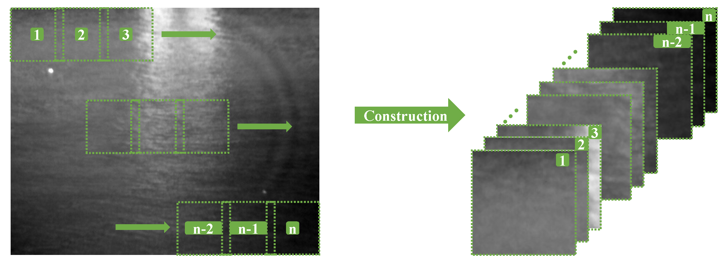
The infrared patch-tensor (IPT) model was proposed by Dai et al. [42]. The patch-tensor is constructed by sliding rectangular patches of the same size on the original image and finally stacking the patches into a three-dimensional tensor cube, as shown in Figure 4. The original expression of the IPT model is as

$$\mathcal{D}=\mathcal{B}+\mathcal{T}+\mathcal{N}$$

(9)

where $\mathcal{D}$ denotes the patch-tensor constructed from the original image; $\mathcal{B}$ denotes the low-rank background patch-tensor; $\mathcal{T}$ denotes the sparse target patch-tensor; and $\mathcal{N}$ denotes the random noise patch-tensor. Then, a tensor robust principle component analysis (TRPCA) [48] problem can be obtained as follows:

$$\underset{\mathcal{B},\mathcal{T}}{min}rank\left(\mathcal{B}\right)+\lambda {\parallel \mathcal{T}\parallel }_0\mathrm{s}.\mathrm{t}.\mathcal{D}=\mathcal{B}+\mathcal{T}$$

(10)

where $\mathrm{rank}(·)$ indicates the rank of a matrix or tensor, $\lambda$ is a compromising parameter, and ${\parallel ·\parallel }_0$ represents the $l_0$-norm. Since solving the $l_0$-norm of a patch-tensor is an NP-hard problem, the $l_1$-norm is used to approximate the $l_0$-norm convexly.

3.2. IPT Model Based on PSTNN

Unlike matrices, the rank of patch-tensor is not uniquely defined. It is important to select a suitable tensor rank with a tight convex relaxation to ensure the speed and accuracy of the solution. Partial sum of the tubal nuclear norm [49] is selected to estimate the rank of patch-tensor. The definition is as follows:

$${∥\mathcal{X}∥}_{\mathrm{PSTNN}}=\sum _{i=1}^n{∥{\overline{X}}^{\left(i\right)}∥}_{p=N}$$

(11)

where ${\parallel ·\parallel }_{\mathrm{PSTNN}}$ represents the estimate of the patch-tensor rank, and n represents the number of patches shown in Figure 4. ${\overline{X}}^{\left(i\right)}$ denotes the matrix obtained by Fourier transformation of the i-th frontal slice of the tensor $\mathcal{X}$, ${\parallel ·\parallel }_{p=N}$ denotes the partial sum of singular values (PSSV) [50]. In order to obtain the ideal N value, $\mathcal{X}$ is decomposed into a matrix along the frontal slice, and we calculate the singular values and set the number of singular values greater than 10% of the maximum singular value to N value [49].

Thus, the low-rank and sparse infrared small target detection model based on PSTNN joint $l_1$-norm is defined as:

$$\underset{\mathcal{B},\mathcal{T}}{\min }{\parallel \mathcal{B}\parallel }_{\mathrm{PSTNN}}+\lambda {\parallel \mathcal{T}\odot \mathcal{W}\parallel }_{1}s.t.\mathcal{D}=\mathcal{B}+\mathcal{T}$$

(12)

where ⊙ indicates the Hadamard product, $\mathcal{W}$ is the final weight tensor, which can be obtained by Equation (13), ${\mathcal{W}}_{rec}$ is the tensor obtained by inverting the elements in ${\mathcal{W}}_p$, sparse weight ${\mathcal{W}}_{sw}$ is a reweighted scheme [51], which is used to improve the accuracy and speed of solving the $l_1$-norm minimization problem and can be calculated by Equation (14), where c is generally set to 1, $\epsilon >0$ is a small number to to prevent the denominator from being zero, and k denotes the number of iterations.

$$\mathcal{W}={\mathcal{W}}_{s\omega }\odot {\mathcal{W}}_{rec}$$

(13)

$${\mathcal{W}}_{s\omega }^{k+1}=\frac{c}{|{\mathcal{T}}^k|+\epsilon }$$

(14)

3.3. Solution of the Proposed Model

As a convex optimization problem-solving method, the alternating direction method of multipliers (ADMM) [52] is currently one of the most efficient methods, so it is applied in this paper to solve the problem in Equation (12). The augmented Langrangian function of Equation (12) can be represented as:

$$L_{\mu }(\mathcal{B},\mathcal{T},\mathcal{W},\mathcal{Y})={∥\mathcal{X}∥}_{\mathrm{PSTNN}}+\lambda {∥\mathcal{T}\odot \mathcal{W}∥}_1+<\mathcal{Y},\mathcal{B}+\mathcal{T}-\mathcal{D}>+\frac{\mu }{2}{∥\mathcal{B}+\mathcal{T}-\mathcal{D}∥}_F^2$$

(15)

where $\mathcal{Y}$ is the Lagrange multiplier, $〈·〉$ denotes the inner product, ${∥·∥}_F$ is the Frobenius norm, and $\mu >0$ is a penalty factor.

Then, the problem ${argmin}_{\mathcal{B},\mathcal{T},\mathcal{W},\mathcal{Y}}{\mathrm{L}}_{\mu }(\mathcal{B},\mathcal{T},\mathcal{W},\mathcal{Y})$ in Equation (15) can be solved by the following several subproblems, $\mathcal{T}$ and $\mathcal{B}$ at $k+1$ step iteration is computed as follows:

$${\mathcal{T}}^{k+1}=\underset{\mathcal{T}}{\mathrm{argmin}}\lambda {∥\mathcal{T}\odot {\mathcal{W}}^k∥}_1+\frac{{\mu }^k}{2}{∥{\mathcal{B}}^k+\mathcal{T}-\mathcal{D}+\frac{{\mathcal{Y}}^k}{{\mu }^k}∥}_F^2$$

(16)

$${\mathcal{B}}^{k+1}=\underset{\mathcal{B}}{\mathrm{argmin}}{\parallel \mathcal{B}\parallel }_{\mathrm{PSTNN}}+\frac{{\mu }^k}{2}{∥\mathcal{B}+{\mathcal{T}}^{k+1}-\mathcal{D}+\frac{{\mathcal{Y}}^k}{{\mu }^k}∥}_F^2$$

(17)

The subproblem (16) is solved via soft thresholding operator [53]:

$${\mathcal{T}}^{k+1}={\mathcal{S}}_{\frac{\lambda {\mathcal{W}}^k}{{\mu }^k}}\left(\mathcal{D}-{\mathcal{B}}^k-\frac{{\mathcal{Y}}^k}{{\mu }^k}\right)$$

(18)

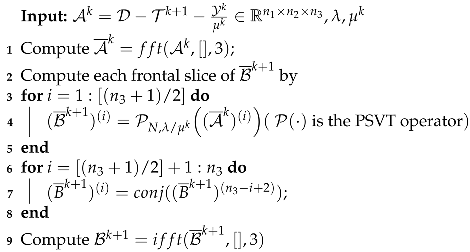
The subproblem (17) is solved via a partial singular value thresholding operator (PSVT) [50] through Fourier fast t-SVD computation, as shown in Algorithm 1 [54]. Then, Y and $\mu$ are updated by:

$${\mathcal{Y}}^{k+1}={\mathcal{Y}}^k+{\mu }^k\left(\mathcal{D}-{\mathcal{B}}^{k+1}-{\mathcal{T}}^{k+1}\right)$$

(19)

$${\mu }^{k+1}=\rho {\mu }^k$$

(20)

Algorithm 1: Solve Equation $\left(17\right)$ using PSVT

The k-th iteration flow of ADMM is shown in Algorithm 2. After the calculation of Algorithm 1, compared with $\mathcal{D}$, the smaller singular values of ${\mathcal{B}}^k$ are suppressed, which inhibits more sparse components and causes more details loss. So, compared with $\mathcal{D}$, the grayscale of sparse components whose grayscale values are higher than local background will descend, yet the grayscale of sparse components whose grayscale values are lower than local background will ascend in ${\mathcal{B}}^k$. Therefore, in Equation (18), there will be some pixels with values less than zero in $\mathcal{D}-{\mathcal{B}}^k-{\mathcal{Y}}^k/{\mu }^k$, which are discarded by the soft thresholding operator that only considers positive elements and default the grayscale of the target as higher than the local background. However, as we have discussed above, the grayscale of the target is not always higher than the local background. The dark targets will be missed by Equation (18). Unfortunately, we can not directly take the absolute value of the result of $\mathcal{D}-{\mathcal{B}}^k-{\mathcal{Y}}^k/{\mu }^k$, because in most cases, targets in the infrared maritime image have uniform polarity. If the absolute value is taken directly, it is bound to introduce some interference with the opposite polarity to the target and then affect the false alarm rate. Therefore, determining the polarity of the target in a certain scene is the key to ensure a low miss rate and false alarm rate.

Algorithm 2: The k-th iteration flow of ADMM

Input:  ${\mathcal{T}}^k,{\mathcal{B}}^k,{\mathcal{Y}}^k,{\mathcal{W}}^k,{\mathcal{W}}_{rec},\mathcal{D},\lambda ,{\mu }^k,\rho =1.1,c=1$ 1 Fix the others and update ${\mathcal{B}}^{k+1}$ by Algorithm 1; 2 Fix the others and update ${\mathcal{T}}^{k+1}$ by Equation $\left(18\right)$; 3 Fix the others and update ${\mathcal{Y}}^{k+1}$ by Equation $\left(19\right)$; 4 Fix the others and update ${\mathcal{W}}^{k+1}$ by 5 ${\mathcal{W}}_{s\omega }^{k+1}=\frac{c}{|{\mathcal{T}}^k|+\epsilon }$ 6 ${\mathcal{W}}^{k+1}={\mathcal{W}}_{rec}\odot {\mathcal{W}}_{s\omega }^{k+1}$ 7 Update $\mu$ by Equation $\left(20\right)$;     Output:  ${\mathcal{T}}^k$, ${\mathcal{T}}^{k+1}$, ${\mathcal{B}}^{k+1}$, ${\mathcal{Y}}^{k+1}$, ${\mathcal{W}}^{k+1}$, ${\mu }^{k+1}$

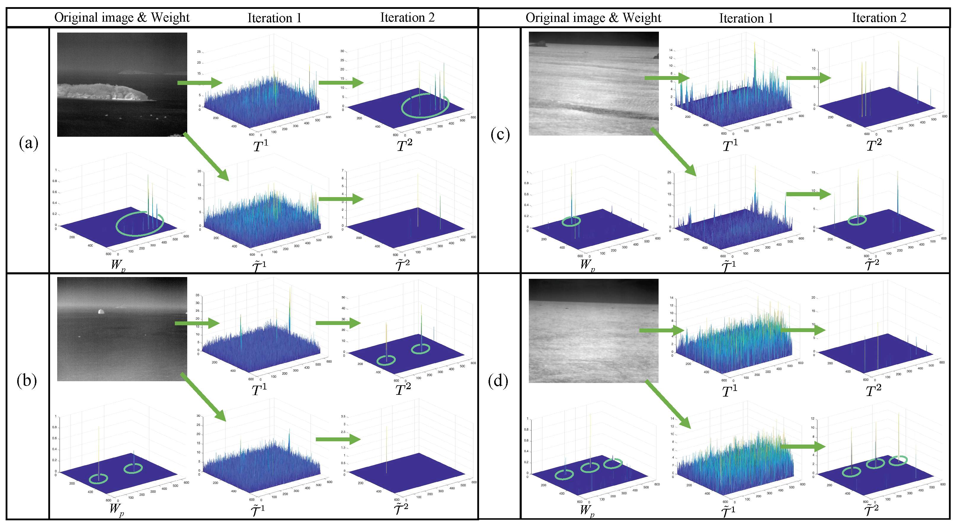
We set the maximum grayscale of D to be 255, and the image of D with its polarity reversed ($255-D$) is defined as $\tilde{D}$. If the polarity of the target in D is negative, substituting $\tilde{D}$ into Equation (12) can ensure that the dark target is not missed. We find that the prior weight $W_p$ is always significant at the target location, regardless of the polarity of the target positive or negative. Therefore, $\mathcal{D}$ and $\tilde{\mathcal{D}}$ can be substituted into Equation (12) to calculate the sparse components with different polarities, and the polarity of the target can be judged by comparing the similarity with ${\mathcal{W}}_p$. However, if $\mathcal{D}$ and $\tilde{\mathcal{D}}$ are iterated to convergence using ADMM and then judged for similarity to ${\mathcal{W}}_p$, this will double the computation time.

We notice that in the iterative process, when $k=2$, the sparse component ${\mathcal{T}}^2$ or ${\tilde{\mathcal{T}}}^2$ is sufficiently separated from $\mathcal{D}$ or $\tilde{\mathcal{D}}$. There is a significant difference between ${\mathcal{T}}^2$ and ${\tilde{\mathcal{T}}}^2$. Therefore, we only need to determine the polarity when $k=2$, which can effectively shorten the running time.

Figure 5 shows the comparison of the sparse components $T^1$, ${\tilde{T}}^1$, $T^2$, ${\tilde{T}}^2$ and $W_p$ for the scene with different polarity targets. It can be seen that after the first iteration, the similarity of $T^1$ and ${\tilde{T}}^1$ to $W_p$ is not well resolved. After the second iteration, in both Figure 5a,b, $T^2$ is clearly more similar to $W_p$, since the targets are of positive polarity; in both Figure 5c,d, ${\tilde{T}}^2$ is clearly more similar to $W_p$, since the targets are of negative polarity. Features whose prior weight $W_p$ is clearly similar to the sparse component $T^2$ or ${\tilde{T}}^2$ are highlighted in the figure.

Since the sparse component with the correct polarity $T^2$ or ${\tilde{T}}^2$ has a higher intensity value at the same position as the prior weight $W_p$, we propose the concept of sparse-weight similarity $s_{sw}$. The sparse components ${\mathcal{T}}^2$ and ${\tilde{\mathcal{T}}}^2$ are obtained by iterating the original image and its grayscale inversion image twice through ADMM. Then, the polarity of the target is determined by comparing their similarity with ${\mathcal{W}}_p$:

$$s_{sw}=\parallel {\mathcal{T}}^2\odot {\mathcal{W}}_p{\parallel }_1,{\tilde{s}}_{sw}={\parallel {\tilde{\mathcal{T}}}^2\odot {\mathcal{W}}_p\parallel }_1$$

(21)

Table 1. The values of $s_{sw}$ and ${\tilde{s}}_{sw}$.

	(a)	(b)	(c)	(d)
$s_{sw}$	21.91	34.01	2.70	3.97
${\tilde{s}}_{sw}$	0.00	0.06	8.04	10.06

shows the values of $s_{sw}$ and ${\tilde{s}}_{sw}$ for each scene of Figure 5. Apparently, when $s_{sw}>{\tilde{s}}_{sw}$, the polarity of the target is positive; when $s_{sw}<{\tilde{s}}_{sw}$, the polarity of the target is negative. After judging the target polarity, the branch with higher sparse-weight similarity continues to iterate, and the other branch stops iteration, which can save a lot of computing time.

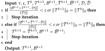
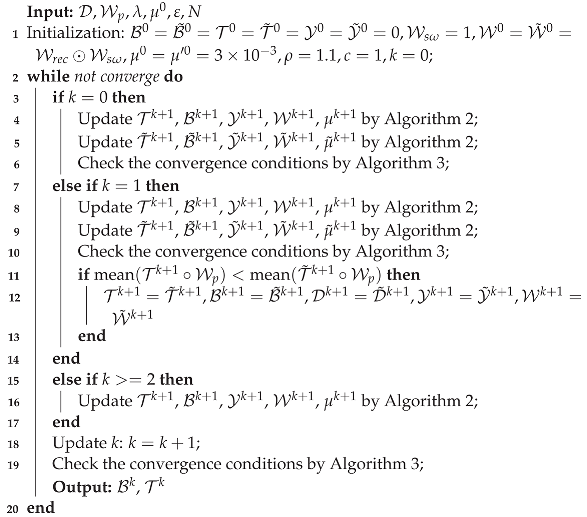
Since the $l_0$-norm of the target patch-tensor will stop changing after several iterations, in order to reduce the running time of the method, the iteration will be stopped when the $l_0$-norm of the target patch-tensor of the two adjacent iterations is equal or the relative error (${\parallel \mathcal{B}+\mathcal{T}-\mathcal{D}\parallel }_F^2{/\mathcal{D}\parallel }_F^2$) is less than a certain threshold, as shown in Algorithm 3. The overall flow of the proposed PSTNN-based and ADMM methods with target polarity judgement is shown in Algorithm 4.

3.4. The Overall Procedure of the Proposed Method

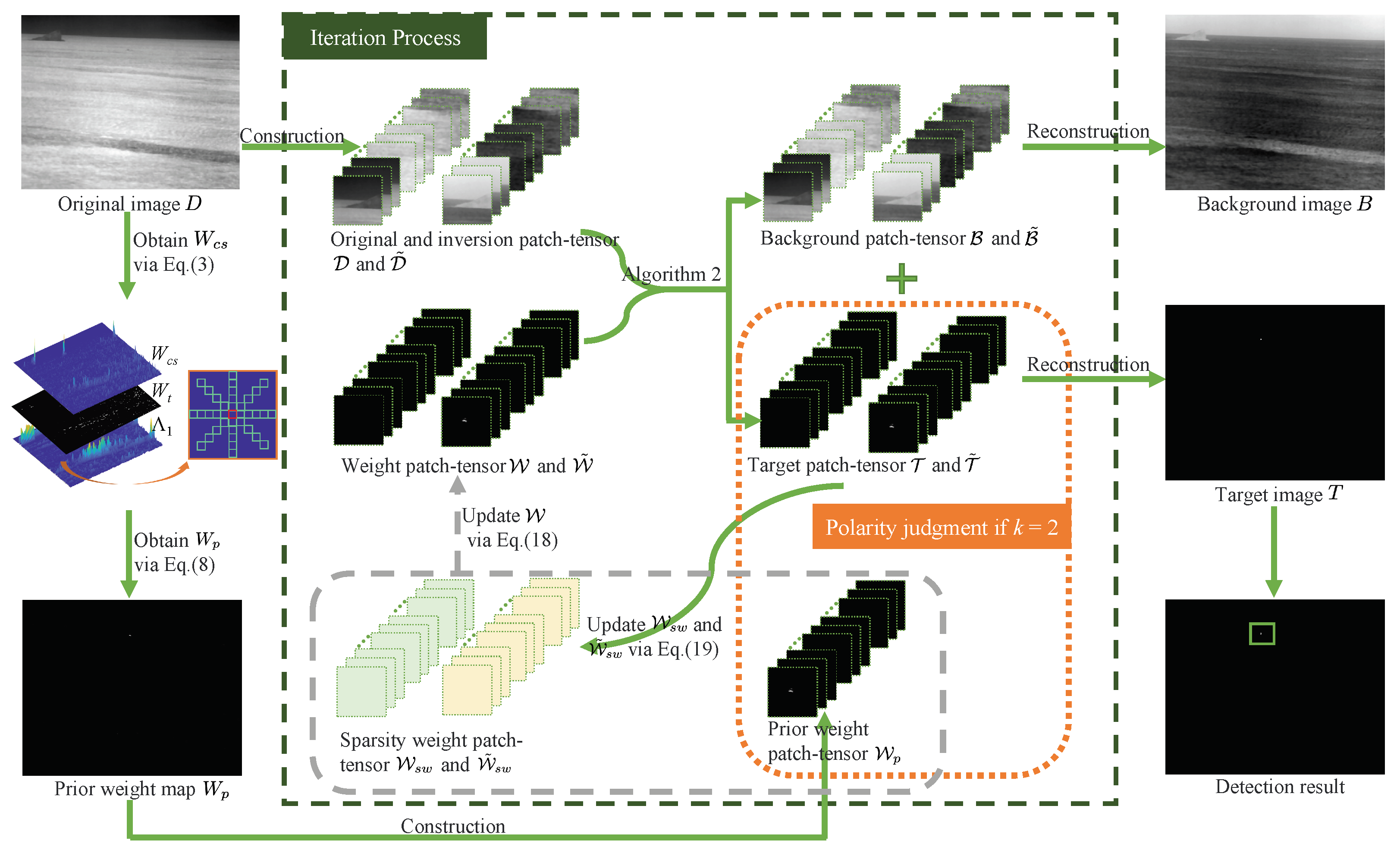
Figure 6 shows the overall procedure of the proposed method, which can be described in the following steps:

• Prior weight extraction. The prior weight map $W_p$ is extracted by Equations (3)–(8) using structure tensor and multidirectional uniformity.
• Patch-tensor construction. The patch-tensors of the original image D and its polarity reversed $\tilde{D}$ and prior weight $W_p$ are constructed by the illustration of Figure 4.
• Target-background separation and polarity judgment. The input patch-tensor $\mathcal{D}$ and $\tilde{\mathcal{D}}$ are decomposed into low-rank patch-tensors $\mathcal{B}$, $\tilde{\mathcal{B}}$ and sparse patch-tensors $\mathcal{T}$, $\tilde{\mathcal{T}}$ by Algorithm 2. The polarity of target is judged by comparing the similarity of the sparse components ${\mathcal{T}}^2$ and ${\tilde{\mathcal{T}}}^2$ with ${\mathcal{W}}_p$ after two iterations.
• Image reconstruction and target extraction. When the iterative process meets the convergence condition in Algorithm 3, the background component B and target component T are reconstructed from the low-rank patch-tensor $\mathcal{B}$ and sparse patch-tensor $\mathcal{T}$. The construction and reconstruction are opposite processes. Finally, the target we need to detect is obtained.

Algorithm 3: Iteration stop judgment

Algorithm 4: The proposed method

4. Experiments and Analysis

In this section, the experimental setup, including the dataset employed in this paper, quantitative evaluation indicators and baseline methods are introduced. Then, the parameters of the proposed method are determined by experiments. The proposed method is compared with baseline methods qualitatively and quantitatively. Finally, the running time of each method is compared.

4.1. Experimental Setup

4.1.1. The Data Set

In this paper, 14 groups of infrared maritime images of different scenes are selected to verify the effectiveness and robustness of the proposed methods. Each image sequence contains 100 frames. The size of each frame in sequence (a) is 284 × 236 and in sequence (b) to (l) is 640 × 512. Typical images in each sequence are shown in Figure 7. Among them, (a) to (e) are the scenes without island and with bright targets. (f) to (i) are the scenes with island, and (i) to (l) are the scenes with dark targets.

Table 2. Detail information contained in 14 different scenes.

	Target Size	Local Mean Contrast
(a)	$12\times 8$	1.1312
(b)	$35\times 14$	1.3652
(c)	$15\times 15,11\times 10$	1.5934, 1.8222
(d)	$11\times 11$	1.0445
(e)	$13\times 6,39\times 10$	1.0895, 1.0846
(f)	$14\times 11$, $15\times 9$, $13\times 8$, $13\times 9$, $15\times 12$, $14\times 11$	2.3491, 2.0108, 1.5586, 1.9523, 2.2617, 2.1364
(g)	$13\times 10$	1.5062
(h)	$12\times 9,10\times 8$	1.3891, 1.2579
(i)	$23\times 5$	0.9782
(j)	$15\times 13,19\times 15$	0.9939, 0.9947
(k)	$10\times 10,28\times 8$	0.9933, 0.9484
(l)	$19\times 7,19\times 8,20\times 7,23\times 7$	0.9859, 0.9674, 0.9722, 0.9477
(m)	$12\times 14,11\times 13$	0.9340, 0.9300
(n)	$15\times 14,15\times 13$	0.9825, 0.9847

shows the target sizes and local mean contrast (LMC) in each sequence. LMC can be calculated by Equation (22), where $\overline{I_t}$ represents the average grayscale of the target area, $\overline{I_b}$ represents the average grayscale of the local background area, and the local background area is obtained by extending the target boundary by 20 pixels.

$$\mathrm{LMC}=\frac{\overline{I_t}}{\overline{I_b}}$$

(22)

4.1.2. Evaluation Metrics

In target detection, MAR, FAR, BSF and SCRG are used as evaluation indexes to evaluate the effect of the method. MAR (Missing Alarm Rate) represents the ratio between the number of missed targets calculated by the method and the number of real targets. FAR (False Alarm Rate) represents the ratio between the number of false targets detected by the method and the number of all detected targets, BSF (Background Suppression Factor) is used to represent the residual degree of background clutter in the image and to characterize the effect of background noise suppression before and after detection. SCRG (Signal-to-Clutter Ratio Gain) is used to evaluate signal-enhanced performance. MAR and FAR can be expressed by the following equations:

$$\mathrm{MAR}=\frac{\mathrm{MT}}{\mathrm{MT}+\mathrm{DT}}\times 100\%$$

(23)

$$\mathrm{FAR}=\frac{\mathrm{FT}}{\mathrm{FT}+\mathrm{DT}}\times 100\%$$

(24)

where MT represents the missed target, DT represents the detected real target, and FT represents the detected false target. BSF and SCRG can be represented by:

$$\mathrm{BSF}=\frac{{\sigma }_{\mathrm{in}}}{{\sigma }_{\mathrm{out}}+c}$$

(25)

$$\mathrm{SCR}=\frac{\left|{\mu }_t-{\mu }_b\right|}{{\sigma }_b+c}$$

(26)

$$\mathrm{SCRG}=\frac{{\mathrm{SCR}}_{\mathrm{out}}}{{\mathrm{SCR}}_{\mathrm{in}}+c}$$

(27)

where $\sigma$ in BSF represents the standard deviation of the hole image except for the target area, in and out represent input and output images, respectively, SCR represents the signal-to-clutter ratio of input or output signals, $\mu$ represents the average intensity of the target or background area, t represents the target, b represents the background, and ${\sigma }_b$ in SCR represents the standard deviation of the local background of target. We set the size of the background in SCR as the area obtained by extending the target area boundary by 20 pixels. c is a small positive constant, which is set as 0.001 in this paper, to avoid the denominator becoming zero [55]. The larger the standard deviation of the image is, the more complex the image is, and the small and weak target is more likely to be submerged in the image with large standard deviation; otherwise, the target will be salient in the image. Therefore, the higher the BSF value of the image, the more obvious the background suppression, and the easier it is to detect the target. The larger the SCRG, the greater the saliency of the target relative to the background, indicating that the target is easier to be detected.

4.1.3. Baseline Method

We selected nine public typical baseline methods and compared them with the methods proposed in this paper to verify the effectiveness of our method, including: YOLOv5 (https://github.com/ultralytics/yolov5 (accessed on 20 July 2022 )), GST [56], FKRW [57], RLCM [19], NRAM [35], NOLC [38], PSTNN [43], SRWS [41], NTFRA [24]. Among them, YOLOv5 is a deep learning method, GST is based on structural tensor, FKRW is based on facet kernel and random walk, RLCM is based on local contrast, NRAM, NOLC, PSTNN, SRWS and NTFRA are based on principal component analysis.

In the comparison test, the parameter settings of each traditional baseline method are shown in

Table 3. Parameter settings for the eight baseline methods.

Methods	Parameter Settings
GST	${\sigma }_1=0.6$, ${\sigma }_2=1.1$, boundary width = 5, filter size = 5
FKRW	$k=4,p=6,\beta =200$, window size: $11\times 11$
RLCM	scale = 3, $K_1=[2,5,9],K_2=[4,9,16]$
NRAM	patch size = 50, slide step = 10, $\lambda =1/\sqrt{\min (m,n)}$, ${\mu }^0=3\sqrt{\min (m,n)}$, $\gamma =0.002$, $C=\sqrt{\min (m,n)}/2.5$
NOLC	patch size = 30, slide step = 10, $\lambda :=L/\sqrt{\max \left(\mathrm{size}\right(D\left)\right)},L=1,p=0.5$
PSTNN	patch size = 40, slide step = 40, $L=0.6$, $\lambda ={\lambda }_L/\sqrt{\min (n_1,n_2)\ast n_3}$
SRWS	patch size = 50, slide step = 50, $\beta =1/\sqrt{\min (m,n)}$, $\lambda ={\lambda }_L/\sqrt{\min (m,n)}$, $\gamma ={\gamma }_L/\sqrt{\min (m,n)}$8
NTFRA	patch size = 40, slide step = 40, $\lambda =1/\sqrt{\min (n_1,n_2)\ast n_3}$

. The parameters of baseline methods are the same as the default parameters in their open-source code except SRWS due to slower speed and non-ideal results.

4.2. Analysis of Parameters

Four different scenes in Figure 1 are selected to discuss the influence of the values of each parameter in the proposed methods on detection results so as to provide a basis for the selection of parameters and obtain the best parameters to achieve the best detection results. Figure 8 shows the impact of six key parameters on the MAR and FAR.

(a) Segmentation threshold k.

In the multidirectional uniformity method proposed in this paper, in order to reduce the running time, a simple adaptive threshold segmentation is first carried out. If the value of k is too large, the target with weak corner strength will be missed, and if it is too small, the running time of the method will be increased. By comparing the curves related to k in Figure 8, it can be seen that a larger value of k increases MAR and a smaller value of k increases FAR, so $k=4$ is taken in this paper to trade off FAR and MAR.

(b) Extended length of multidirectional uniformity $l_e$.

It is necessary to determine the extended length $l_e$ when constructing the element-wise local multidirectional vectors. If the value of $l_e$ is too small to cover the size of the target, the target will be missed; if the value of $l_e$ is too large, other edge interference may be introduced when constructing multidirection vectors centered on the target, which will lead to missed detection. By comparing the curves related to $l_e$ in Figure 8, when $l_e\ge 12$, both the FAR and the MAR are relatively low. Considering that the value of $l_e$ should not be too large, $l_e=12$ is chosen as the final value in this paper

(c) Patch size.

The size of the patch in Figure 4 affects the accuracy and complexity of the method. When the patch size is large, the target has better sparsity and is easier to be separated from the background. When the patch size is small, the complexity of singular value decomposition of each patch will be reduced. By comparing the curves related to patch size in Figure 8, the ideal effect is achieved when the patch size=40, so the patch size is set as 40 in this paper.

(d) Sliding step.

The sliding step in the construction of patch-tensor should not be too small. A too small sliding step will result in insufficient sparsity of the target and increase the running time. Meanwhile, the distance should not be larger than the patch size to ensure that all information in the image is not lost. By comparing the curves related to the sliding step in Figure 8, the ideal effect is achieved when the sliding step = 40, so the sliding step is set as 40 in this paper.

(e) Penalty Factor $\mu$.

$\mu$ controls the tradeoff between the low-rank and sparse tensors. If the value of $\mu$ is too small, more sparse components will remain in the low-rank background, resulting in an increase in MAR. If the value of $\mu$ is too large, the more background interference will be extracted into the sparse component, leading to an increase in FAR. By comparing the curves related to $\mu$ in Figure 8, the ideal effect is achieved when $\mu =3\times {10}^{-3}$, so $\mu$ is set as $3\times {10}^{-3}$ in this paper.

(f) Compromising Parameter $\lambda$.

$\lambda$ also controls the tradeoff between the low-rank and sparse tensors, which is set as $L/\sqrt{\max (n_1,n_2)\ast n_3}$ with reference to [48] ($n_1$, $n_2$ and $n_3$ denote the length, width and number of patches, respectively). By comparing the curves related to L in Figure 8, it can be seen that when L increases, MAR tends to increase, and when L decreases, FAR tends to increase. Therefore, $\lambda$ is set as $0.6/\sqrt{\max (n_1,n_2)\ast n_3}$ in this paper.

4.3. Accuracy of Polarity Judgment

The sparse-weight similarity to judge the polarity of the target proposed in this paper is not completely accurate, especially in some scenes with obvious sparse interference opposite to the polarity of the target. We counted the polarity judgment error rates $r_e$ for the 14 sequences in Figure 7, as shown in

Table 4. The polarity judgment error rates $r_e$ of 14 sequences.

	(a)	(b)	(c)	(d)	(e)	(f)	(g)	(h)	(i)	(j)	(k)	(l)	(m)	(n)
$r_e$	0%	0%	0%	2%	3%	0%	0%	0%	5%	10%	5%	7%	0%	0%

. Combined with Figure 7, it can be seen that there are a large number of negative polarity wave clutter in sequences (d) and (e), and a large number of positive polarity wave clutter in (i)–(l), leading to a certain amount of wrong judgments.

4.4. The Qualitative Comparison

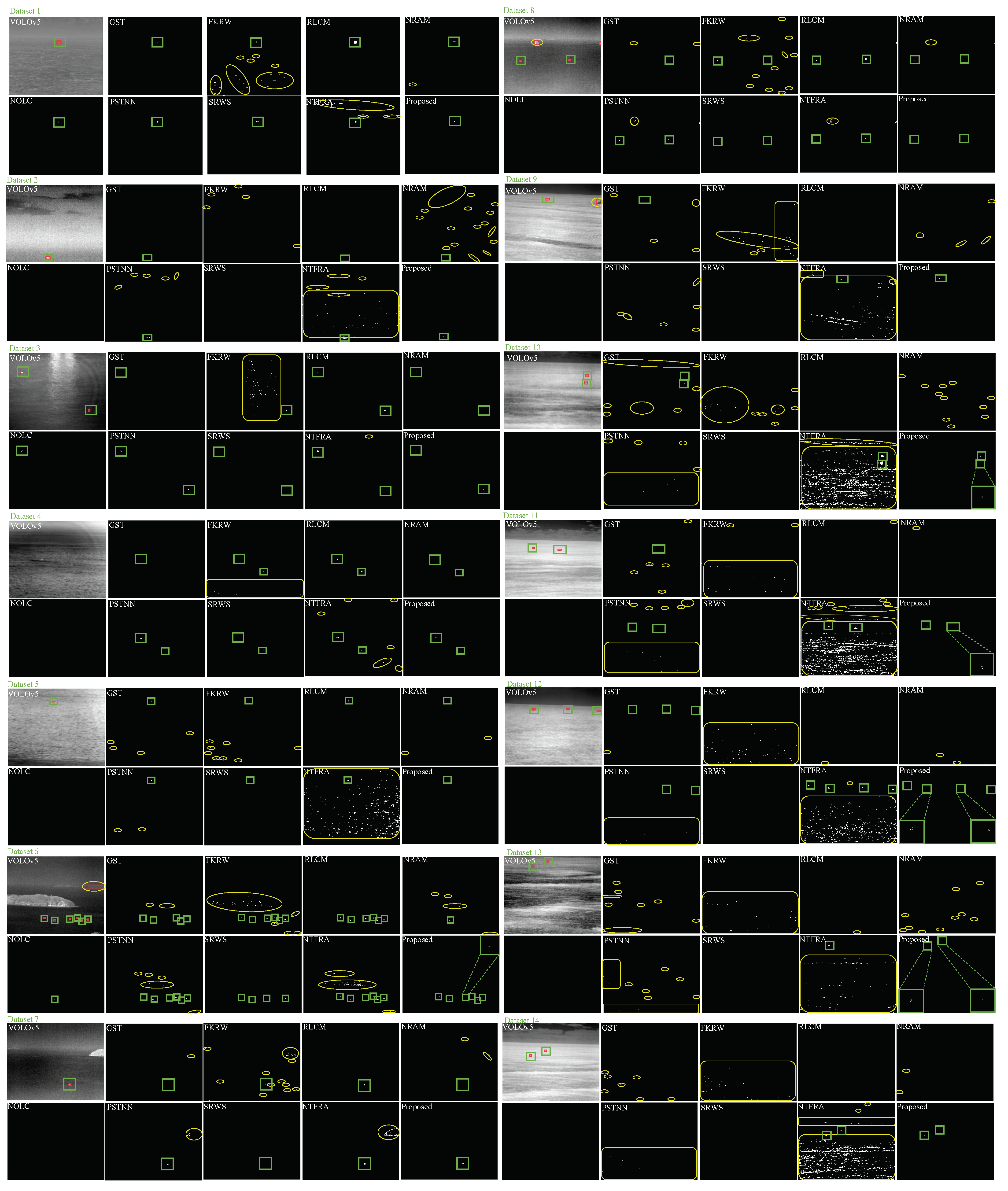
After determining the values of the parameters of the proposed method, we compared the detection results of nine baseline methods and the proposed method in 14 different sequences in Figure 7 and show representative single frame results in Figure 9. It can be seen in traditional methods that FKRW and NTFRA have higher FAR and are easily disturbed by wave clutter, while NOLC and SRWS have higher MAR. When detecting sequences with strong island edges, RLCM and the proposed method have a high suppression effect, while GST, FKRW, NRAM, PSTNN, NTFRA have a relatively poor suppression effect. Although RLCM has a good effect in detecting targets with positive polarity, the morphology of the targets is lost. When detecting sequences with negative polarity targets, GST, PSTNN, NTFRA can detect part of negative polarity targets, but they are accompanied by a large number of false alarms. VOLOv5 has a significant effect on background clutter suppression, and the main source of false alarm is misjudging islands as targets. At the same time, the phenomenon of missing detection appears in a few scenes. Due to the low multidirectional uniformity at the edge of the target, the proposed method will cause the target to shrink to a certain extent. In summary, the proposed method achieves strong robust detection for scenes with strong island edge and targets with different polarities at the cost of shrinking the detected target size.

4.5. The Quantitative Comparison

In this paper, MAR, FAR, BSF and SCRG are used to measure the detection effect of the baseline methods and the proposed method.

Table 5. Comparison of average MAR between the proposed method and 9 baseline methods in 14 sequence scenes.

	VOLOv5	GST	FKRW	RLCM	NRAM	NOLC	PSTNN	SRWS	NTFRA	Proposed
Dataset 1	0%	0%	0%	0%	0%	0%	0%	0%	0%	0%
Dataset 2	0%	5%	11%	0%	30%	100%	2%	86%	5%	0%
Dataset 3	0%	28.5%	30%	0%	15%	21.5%	1.5%	10%	6.5%	0%
Dataset 4	26.5%	81.5%	5%	0%	15%	45%	0%	33.5%	3.5%	1.5%
Dataset 5	0%	2%	2%	0%	0%	0%	60%	0%	10%	3%
Dataset 6	0%	8.33%	0%	0%	77.17%	93.17%	0%	14.33%	1.5%	0%
Dataset 7	0%	14%	0%	0%	8%	92%	13%	3%	14%	0%
Dataset 8	0%	56%	3%	0%	1.5%	86.5%	0%	10.5%	0%	0%
Dataset 9	0%	0%	66%	100%	34%	79%	34%	79%	0%	5%
Dataset 10	3.5%	4.5%	81%	100%	44.5%	82%	21%	83%	0%	11%
Dataset 11	4.5%	41.5%	85.5%	100%	73.5%	86.5%	23.5%	87.5%	0%	5.5%
Dataset 12	1.25%	24.5%	100%	100%	67.75%	100%	15.75%	88.75%	0%	7.75%
Dataset 13	0%	94.5%	100%	100%	100%	100%	100%	100%	44.5%	0%
Dataset 14	0%	94%	100%	100%	96%	100%	100%	100%	0%	0.5%

Bold indicates that the proposed method is better than the baseline methods. Underline indicates that the proposed method is better than the baseline methods by combining both MAR and FAR.

,

Table 6. Comparison of average FAR between the proposed method and 9 baseline methods in 14 sequence scenes.

	VOLOv5	GST	FKRW	RLCM	NRAM	NOLC	PSTNN	SRWS	NTFRA	Proposed
Dataset 1	0%	0%	96.22%	0%	22.48%	5.66%	4.76%	0%	89.79%	0%
Dataset 2	2.91%	5.66%	92.34%	0%	97.88%	100%	0.99%	0%	99.05%	0%
Dataset 3	0.99%	0%	98.59%	4.67%	15.25%	2.07%	0%	1.48%	75.76%	0%
Dataset 4	0.68%	0%	95.53%	0%	15.91%	2.44%	9.13%	2.10%	96.40%	1.48%
Dataset 5	6.49%	68.85%	93.80%	0%	24.10%	10.91%	7.41%	5.32%	99.81%	6.25%
Dataset 6	6.54%	47.69%	90.63%	0%	86.48%	26.81%	78.88%	0%	87.65%	0%
Dataset 7	37.5%	70.15%	94.29%	0%	82.79%	86.45%	93.14%	14.85%	94.35%	0%
Dataset 8	33.3%	77.14%	92.40%	37%	78.49%	0%	84.36%	0%	98.38%	0%
Dataset 9	21.88%	83.90%	99.24%	NaN	83.20%	0%	98.37%	0%	99.89%	11.50%
Dataset 10	0%	93.80%	99.49%	NaN	89.75%	0%	99.35%	0%	99.89%	9.91%
Dataset 11	0%	91.46%	99.71%	100%	96.55%	0%	99.34%	0%	99.88%	8.26%
Dataset 12	0%	79.66%	100%	100%	86.11%	NaN	98.33%	0%	99.80%	4.08%
Dataset 13	0%	99.28%	100%	100%	100%	NaN	100%	NaN	99.58%	1.48%
Dataset 14	0%	99.45%	100%	NaN	96.86%	100%	100%	NaN	99.78%	1.97%

Bold indicates that the proposed method is better than the baseline methods. NaN indicates that the absence of any detections results in a denominator of zero. Underline indicates that the proposed method is better than the baseline methods by combining both MAR and FAR.

,

Table 7. Comparison of average BSF between the proposed method and 8 traditional baseline methods in 14 sequence scenes.

	GST	FKRW	RLCM	NRAM	NOLC	PSTNN	SRWS	NTFRA	Proposed
Dataset 1	4.96	1.28	4.96	3.08	3.23	3.19	4.96	0.36	4.96
Dataset 2	13.53	3.34	15.18	3.27	14.25	13.35	15.18	1.88	15.18
Dataset 3	35.11	9.29	19.29	20.52	21.60	35.11	21.54	13.59	35.11
Dataset 4	7.67	2.50	7.67	6.68	7.63	7.12	7.60	2.40	7.58
Dataset 5	8.82	4.57	17.92	12.84	13.67	11.34	13.61	0.54	12.98
Dataset 6	9.16	10.82	31.43	8.78	29.10	3.76	31.43	1.37	31.43
Dataset 7	6.96	5.38	19.44	8.14	14.34	2.62	17.43	0.96	19.44
Dataset 8	1.63	2.51	1.69	1.90	5.75	1.14	5.75	0.32	5.75
Dataset 9	2.38	0.88	7.48	3.06	7.48	1.40	7.48	0.24	6.83
Dataset 10	1.95	0.90	7.12	2.84	7.12	1.31	7.12	0.23	6.79
Dataset 11	2.58	1.20	12.57	3.42	11.03	1.48	11.03	0.39	10.45
Dataset 12	2.64	1.13	10.12	4.89	12.47	1.02	12.47	0.44	12.01
Dataset 13	2.80	1.88	13.50	5.27	17.63	2.59	17.63	0.84	17.42
Dataset 14	2.05	1.33	14.86	6.81	14.79	1.50	14.86	0.49	14.68

Bold indicates that the proposed method is better than the baseline methods. Underline indicates that the proposed method is better than the baseline methods by combining both BSF and SCRG.

and

Table 8. Comparison of average SCRG between the proposed method and 8 traditional baseline methods in 14 sequence scenes.

	GST	FKRW	RLCM	NRAM	NOLC	PSTNN	SRWS	NTFRA	Proposed
Dataset 1	1.79	2.67	32.19	4.26	3.00	5.43	2.90	5.89	16.04
Dataset 2	0.64	1.00	2.45	0.06	0	3.55	0.04	13.74	1.69
Dataset 3	1.06	1.50	17.09	1.95	1.37	3.75	1.47	4.99	1.72
Dataset 4	5.94	13.04	88.49	6.48	2.73	27.77	3.77	48.33	49.34
Dataset 5	18.90	32.35	246.35	13.28	1.13	42.59	6.47	76.12	15.56
Dataset 6	0.71	1.67	4.34	0.08	0.02	2.07	0.51	1.65	1.21
Dataset 7	1.36	3.00	10.44	1.43	0.02	6.21	0.84	7.72	3.85
Dataset 8	1.89	2.49	13.06	2.18	0.45	3.99	0.91	7.42	3.77
Dataset 9	10.67	0.59	0	3.62	0.44	2.77	0.55	141.13	36.64
Dataset 10	9.52	0.42	0	3.23	0.44	2.73	0.55	135.05	1.26
Dataset 11	8.42	0.42	0	1.55	0.44	6.37	0.55	77.57	8.01
Dataset 12	42.53	0	0	1.74	0	16.56	0.55	73.29	27.63
Dataset 13	0.60	0	0	0	0	0	0	35.80	4.03
Dataset 14	0.17	0	0	0.08	0	0	0	102.93	12.36

Underline indicates that the proposed method is better than the baseline methods by combining both BSF and SCRG.

, respectively, show the comparison of average values of MAR, FAR, BSF and SCRG calculated by different baseline methods and proposed methods for 14 different sequence scenes. Each sequence contains 100 frames. For BSF and SCRG, the input image is the original image, and the output image is the image of the final result after normalization and before binarization.

From the calculation results of the four parameters of MAR, FAR, BSF and SCRG, it can be seen that FKRW and NTFRA have high FAR in most scenes, NOLC and SRWS have high MAR in most scenes, and RLCM shows better detection results in scenes with positive polarity targets. Most of the methods do not have the ability to detect negative polarity targets. Although GST, RLCM and PSTNN can detect some negative polarity targets, they are accompanied by a large number of false alarms. VOLOv5 shows excellent results on many datasets and is not affected by the polarity of the target but shows high MAR and FAR on some specific datasets. Compared with other methods, the detection effect of the proposed method for negative polarity target is significant. However, compared with RLCM and PSTNN which have a better detection effect on positive polarity target, the proposed method causes some false and misalarm when detecting the positive polarity target in some cases. There are strong interferences of opposite polarity to the target in the corresponding datasets, which causes the wrong judgment of the polarity of the target. From the calculation results of BSF, it can be seen that YOLOv5 shows significant background suppression ability, although some islands are wrongly targeted. The suppression ability of the proposed method to the background interference is stronger than most traditional baseline methods. In order to suppress the strong edge islands, the multidirection uniformity method causes the target result to shrink, which leads to the proposed method having no obvious advantage compared with other methods in SCRG results. Although the results of the proposed method are not the best on some sequences when measuring either BSF or SCRG separately, the proposed method is still a better choice compared to other baseline methods when considering both BSF and SCRG parameters, which are underlined in the table. Combining the four parameters of FAR, MAR, BSF and SCRG, it can be concluded that the proposed method is more robust, can adapt to more complex scenes and has a wider range of application compared with traditional baseline methods.

4.6. Runtime Comparison

All experiments in this paper are run on a MAC computer with 2 GHz quad-core Intel Core I5 CPU and 16 GB memory. The codes of the traditional methods are implemented in MATLAB 2022a. The codes of VOLOv5 are implemented in PyCharm 2022.2. The average runtimes of the proposed method and nine other baseline methods for sequences (a) to (n) are calculated and shown in

Table 9. Comparison of average runtime between the proposed method and 8 baseline methods in 14 sequence scenes.

	GST	FKRW	RLCM	NRAM	NOLC	PSTNN	SRWS	NTFRA	VOLOv5	Proposed
runtime	0.015	0.149	13.445	27.384	3.294	0.387	1.761	3.548	0.258	0.397

. It can be seen that the runtime of the proposed method is relatively short. Let the size of the input image be $M\times N$, the size of the patch-tensor be $n_1\times n_2\times n_3$, the size of the sliding window in multidirectional uniformity be l, and x be the number of nonzero elements in Equation (5), which is a small number compared with $MN$. In the calculation of multidirectional uniformity, a sliding window is used to traverse every nonzero element in the whole image, which needs an $O(x\times l^2)$ cost. The main consumption in PSTNN lies in SVD and FFT, which requires $O(n_1{n}_2{n}_3\log \left(n_1{n}_2\right)+n_1{n}_2^2[(n_3+1)/2])$ cost, so the total computation cost of the proposed model is $O(x\times l^2+n_1{n}_2{n}_3\log \left(n_1{n}_2\right)+n_1{n}_2^2[(n_3+1)/2])$. Methods based on component analysis can greatly reduce the running time by GPU accelerated methods [58]. We implemented the proposed method on VS2015 by GPU acceleration technology on the server equipped with an infrared detection system in the laboratory. After acceleration, the average processing time of each frame of 14 sequential scenes is 0.047 s, which can meet the requirements of real-time monitoring in engineering.

5. Discussion

There is still room to improve the accuracy of infrared maritime target detection. The biggest challenge lies in the unexpected complex background and strong interference. The method based on background estimation filtering and the method based on local features make use of the global information and local information of the image, respectively, which have certain deficiencies. The optimization method based on local feature weight and structure tensors takes full account of global and local information and shows strong robustness. Some islands in infrared maritime images often cause a lot of false alarms because of their obvious edges. It is critical to reduce these interferences without affecting the intensity of the target. Therefore, we take advantage of the characteristic that the eigenvalue ${\Lambda }_1$ of the structure tensor has obvious edges features and propose the multidirectional uniformity to suppress the strong edges. Although the size of the target is shrunk to a certain extent, the detection accuracy is greatly improved. In addition, most of the methods neglect the case that the target grayscale is lower than the background, which leads to the lack of robustness in practical applications. Therefore, it is particularly important to achieve target detection with unknown polarity. The strategy of substituting images of opposite polarities into the optimization algorithm, respectively, and making polarity judgment in the second iteration and stopping the wrong polarity iteration is adopted, which can accurately judge polarity and ensure the effectiveness. After comparing with the advanced baseline methods on a large number of datasets, it can be concluded that the proposed method is more robust, although there are a small number of cases of polarity judgment errors. Deep learning-based methods also show excellent results, although the current infrared maritime datasets are still insufficient. In the future, our research focus will fall on more accurate polarity judgment and control the missed detection rate and false alarm rate in a lower range. In addition, we will consider the use of deep learning methods to obtain stronger robustness while expanding the dataset.

6. Conclusions

In this paper, an infrared maritime target detection method based on multidirectional uniformity and sparse-weight similarity is proposed. In order to detect targets of unknown polarity in infrared maritime images with strong edge interference, firstly, the problem of small infrared target detection is transformed into solving sparse and low-rank components by the TRPCA model. Due to the weak ability of suppressing strong edge interference by the prior weight obtained based on the structure tensor, the strong edge interference in the corner strength map is suppressed by constructing the elementwise scattering filed in eigenvalue ${\Lambda }_1$ and calculating the multidirectional uniformity. PSTNN is used to estimate the rank of the background patch-tensor, and ADMM with target polarity judgment based on sparse-weight similarity is used to solve the optimization model by substituting in images of opposite polarities simultaneously. In order to reduce the complexity of the method, only the polarity of the target is judged in the second step of the iterative process, and the whole method process is designed. By comparing with nine advanced methods on 14 different datasets, the proposed method shows strong robustness, which has a wide range of engineering application value.