Article

Assessing the Performance of WRF Model in Simulating Heavy Precipitation Events over East Africa Using Satellite-Based Precipitation Product

by
Isaac Kwesi Nooni
1,
Guirong Tan
2,
Yan Hongming
3,*,
Abdoul Aziz Saidou Chaibou
4,
Birhanu Asmerom Habtemicheal
4,5,
Gnim Tchalim Gnitou
1 and
Kenny T. C. Lim Kam Sian
1
1
Binjiang College, Nanjing University of Information Science and Technology, Wuxi 214105, China
2
Collaborative Innovation Center on Forecast and Evaluation of Meteorological Disasters, Key Laboratory of Meteorological Disaster, Ministry of Education, Nanjing University of Information Science and Technology, Nanjing 210044, China
3
Yunnan Climate Center, Kunming 650034, China
4
Collaborative Innovation Centre on Forecast and Evaluation of Meteorological Disasters, Key Laboratory for Aerosol-Cloud-Precipitation of China Meteorological Administration, School of Atmospheric Physics, Nanjing University of Information Science and Technology, Nanjing 210044, China
5
Department of Physics, Wollo University, Dessie P.O. Box 1145, Ethiopia
*
Author to whom correspondence should be addressed.
Remote Sens. 2022, 14(9), 1964; https://doi.org/10.3390/rs14091964
Submission received: 21 March 2022 / Revised: 15 April 2022 / Accepted: 17 April 2022 / Published: 19 April 2022

Abstract

:
This study investigated the capability of the Weather Research and Forecasting (WRF) model to simulate seven different heavy precipitation (PRE) events that occurred across East Africa in the summer of 2020. The WRF model outputs were evaluated against high-resolution satellite-based observations, which were obtained from prior evaluations of several satellite observations with 30 stations’ data. The synoptic conditions accompanying the events were also investigated to determine the conditions that are conducive to heavy PRE. The verification of the WRF output was carried out using the area-related root mean square error (RMSE)-based fuzzy method. This method quantifies the similarity of PRE intensity distribution between forecast and observation at different spatial scales. The results showed that the WRF model reproduced the heavy PRE with PRE magnitudes ranging from 6 to >30 mm/day. The spatial pattern from the Precipitation Estimation from Remotely Sensed Information using Artificial Neural Networks-Cloud Classification-Climate Data Record (PERSIANN-CCS-CDR) was close to that of the WRF output. The area-related RMSE with respect to observation showed that the error in the model tended to reduce as the spatial scale increased for all the events. The WRF and high-resolution satellite data had an obvious advantage when validating the heavy PRE events in 2020. This study demonstrated that WRF may be used for forecasting heavy PRE events over East Africa when high resolutions and subsequent simulation setups are used.

1. Introduction

Globally, extreme precipitation (PRE) has increased with the changing nature of the climate. This has led to increasing incidence of flash floods [1]. As a natural disaster, flash floods have devastating impacts on different sectors of society. An example is the socio-economic damage caused by flash floods due to heavy PRE events in Germany (2021), the USA (2021), France (2021), China (2021), and Africa (2019, 2020, and 2021) [2,3]. A flash flood is defined as a sudden and rapid response to a heavy PRE event [1]. Typically, flash flood events are regional or local, and the most vulnerable communities are those with a heavy concentration of buildings and people [1] and weak coping strategies for disasters [1,4,5,6].
Urban flash flooding is a major natural disaster in African countries [7]. A recent review revealed that increased flood risk may persist due to global warming [8]. This indicates that to improve resilience and adaptation to climate uncertainties and provide real-time climate and weather information, a better understanding of the weather system and its drivers is crucial [9]. However, hydrometeorology information on the weather forecast and subsequent flash flood forecasting is poor and inadequate in nearly 80% of African countries [9].
PRE is a challenging weather or climate variable to forecast [10]. However, advances in numerical weather prediction (NWP) have improved our weather forecasting ability, largely due to higher computing power and progress in our understanding of the model dynamics and physics [11,12]. Thus, the ability of the numerical model to correctly represent synoptic conditions and/or simulate specific meteorological episodes strongly depends on the performance of parameterization schemes, as well as lateral and initial boundary conditions [11]. There are many studies that have used WRF in different parts of the world, including Africa. Most of them, however, have focused on seasonal or annual time scales. What is relevant to highlight is that there are not many studies that have conducted high-resolution simulations of heavy rainfall events fully representing small-scale forcings and atmospheric processes (such as convection) [13,14]. Conventionally, numerical model outputs are validated against station measurements [15]. This is widely recommended as the best practice and the benchmark for many model validation studies [11,16]. Denser weather station networks produce robust validation results (assuming the data records are consistently updated) [9,16]. Studies of such a nature are predominantly conducted in developed countries where budgetary allocation for research and development is high [16,17]. The case is completely different for developing countries due to the lack of access to weather station records [17,18,19,20]. This, among other factors (see Nicholson [21]), has become a disincentive for academic research capabilities in the region, thus widening the scientific research gap between African and developed countries.
To address these challenges, satellite PRE products have been proposed as useful proxies for gauged observations [19]. In recent times, policymakers, Earth observation scientists, and engineers from the National Aeronautics and Space Administration (NASA) and European Space Agency (ESA) have advised that the untapped potential of space may provide a breakthrough in how we address climate change threats and challenges [1,22]. As a result, numerous dedicated satellites have been launched into space in the past few decades to serve this purpose [22,23].
Numerous Earth observations are available at different scales. They have been used to monitor, understand, model, and predict climate change-related disasters (see [24,25]). For example, high-resolution satellites can capture at a finer scale local climate information to help us explain and understand climate events [22,23].
Due to the lack of access to weather station records in many African countries, the question on the minds of researchers is whether high-resolution satellite PRE products can be used as proxies to validate numerical model outputs [10]. If so, could the recent multiple heavy PRE episodes and subsequent flash floods that engulfed parts of African countries in the summer of 2020 be used as case studies to explore and understand these products?
High-resolution satellite observations, such as the Tropical Applications of Meteorology using Satellite and Ground-based Observations (TAMSAT, [26]), Precipitation Estimation from Remotely Sensed Information using Artificial Neural Networks-Cloud Classification-Climate Data Record (PERSIANN-CCS-CDR, [27]), Climate Hazards Group Infrared Precipitation with Stations (CHIRPS) [28], and the Integrated Multi-satellitE Retrievals for the Global Precipitation Measurement Mission (GPM IMERG) [29], are publicly available for such research purposes. Many satellite datasets have been validated against gauge observations across Africa at different spatio-temporal scales. For example, validation studies show that these satellite PRE products are consistent with gauge estimates in the Congo [17,30], Kenya [31,32], Ghana [33], and Burkina Faso [34].
Another way to understand heavy PRE events is to investigate the physical mechanisms accompanying them. Many studies have used observational data or numerical modeling [35,36,37]. Established modeling centers, such as the European Centre for Medium-Range Weather Forecasts (ECMWF) [38] or the National Centers for Environmental Prediction (NCEP) [39], provide reanalyses of atmospheric parameters for this purpose [35,36,37,40]. To achieve this, forecasters or modelers use atmospheric parameters as evidence to indicate favorable conditions for a heavy PRE. Local weather conditions are complex, and our understanding of the synoptic conditions over a region of interest (ROI) is incomplete in the literature and teaching. Thus, this approach is helpful and serves as an alternative tool to increase confidence in model simulations or detect discrepancies between simulated and observed estimations. Moreover, this approach can provide more insights into the atmospheric conditions that led to the devastating heavy PRE events in Africa in the summer of 2020.
In the context of the ongoing global warming discussions and the subsequent gap in academic research across Africa, our understanding of routine weather forecasting and warnings is still an open question [22]. This study compared the WRF model outputs against good-performing high-resolution satellite estimates obtained through a preliminary gauge-based evaluation and explored the physical mechanisms accompanying heavy PRE. The outcome may contribute to building the confidence of multi-disciplinary users in the accuracy and reliability of existing tools and products.
Heavy PRE affected East Africa, including Sudan, South Sudan, Ethiopia, Kenya, and Uganda, in the summer of 2020. These episodes are typical heavy PRE events caused by convective activities [2,3] and are common during June, July, August, and September [41]. These events caused flash flooding (with associated fatalities) in East Africa but received little attention from governments or aid agencies [42,43,44].
The main objectives of this study could be summarized as follows: (1) to examine the capability of the WRF model to simulate heavy PRE events; and (2) to investigate the synoptic conditions accompanying the heavy PRE events during the summer of 2020.
The remainder of this paper is divided into four main sections. Section 2 briefly presents the study area, the observational datasets, the WRF model experiment, and the synoptic analysis of severe weather events. Section 3 presents the results, while Section 4 and Section 5 provide the discussions and conclusions, respectively.

2. Materials and Methods

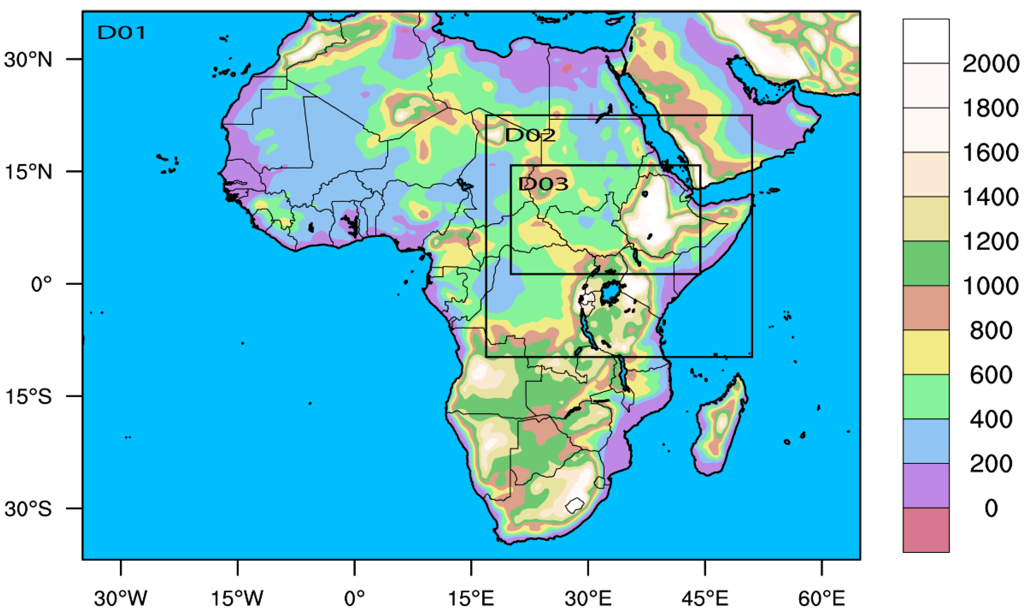
2.1. Study Area, and Heavy PRE Event Selection and Verification

In 2020, seven heavy summer PRE events over East Africa led to flash floods with associated fatalities [2,3]. We relied on two freely available databases to obtain flash flood event information: the Copernicus floodlist web portal [2] and the International Disaster Database (EM-DAT) [3]. Table 1 provides more information on the major events, including the occurrence dates and affected countries.
This study focused on the PRE (June–July–August–September, JJAS) season, mainly in Sudan, South Sudan, Eritrea, Djibouti, and Somalia and extending to some parts of northwestern Ethiopia, eastern Kenya, and northwestern Uganda [8,45]. Most of the events occurred on the South Sudan–Ethiopia border; however, case event 5 affected a larger region, including Kenya, Uganda, and Sudan (Table 1).

2.2. Observation and Model Data

Four (4) high-resolution gridded satellite PRE products, namely TAMSAT [26,46], PERSIANN-CCS-CDR [27,47], CHIRPS [28], and GPM IMERG [29], were used in this study. The satellite PRE data were used as proxies for gauged observations due to data inaccessibility or low density of weather stations over the study region (Table 2).
We first conducted an evaluation study of the four satellite datasets to assess their reliability over the region. The evaluation study used 4 years (2013–2016) of station data over Kenya. Kenya was chosen as the sample sub-area of the study domain because of its relatively good representativity of East Africa’s major climate features and drivers and data availability challenges over the region. The data were obtained from 30 gauge stations distributed over Kenya and sourced by the Kenya Meteorological Department (KMD) (Table S1). The data were screened, quality controlled, and deemed reliable for the validation study. The validation statistics were performed at daily and monthly timescales. It should be noted that the purpose of the evaluation was not to determine the best data but to demonstrate the good performance of the datasets for estimating heavy PRE due to their differences in spatial and temporal resolutions. Following Lockhoff et al. [48], this study considered standard percentile thresholds for extremes and defined extreme PRE events as daily totals exceeding 95th percentiles of the overall daily wet event distribution, estimated from the 30 stations in the period 2013–2016.
Since our primary focus was the 2020 flashfloods, we employed [49] the fuzzy method-based forecast verification. Given the known dependencies between extreme events and simulation resolution, we adopted the area-related root mean square error (RMSE) (Equation (S1)) method proposed by Rezacova et al. [50]. Each scale results in a fixed number of spatial windows for the forecast and observation. For each spatial window, the RMSE is computed between the sorted distribution of pixels within the spatial windows in the forecast and the corresponding sorted distribution of pixels within the same spatial windows in the observation. In this study, the averaged area-related RMSE was calculated for 5, 15, 30, 60, 75, 120, 150, and 240 km scales using the WRF output and PERSIANN-CCS-CDR observational data for all seven events. We considered a 1 mm threshold as a meaningful error and filtered the RMSE matrices before averaging the values.
To investigate the physical mechanism, we used ERA5 atmospheric parameters (see Section 2.4 for details) from ECMWF [38,51] for synoptic analyses. We re-gridded the satellite data resolution to match the WRF inner domain resolution (0.045° × 0.045°) for comparison purposes using a bilinear interpolation technique. ERA5 data were used at a spatial resolution of 0.25° × 0.25°.
Table 2. List of gridded precipitation datasets used in this study.
Type of
Dataset
Spatial ResolutionTemporal ResolutionSourceDownloadable at
SatellitePERSIANN-CCS-CDR0.04° × 0.04°Daily [52][47]
GPM IMERG0.1° × 0.1°Daily[29][53]
CHIRPS0.05° × 0.05°Daily[28][54]
TAMSAT0.0375° × 0.0375°Daily[26][46]
WRFD01
D02
D03
0.405° × 0.376°
0.135° × 0.132°
0.045° × 0.045°
3-hourly[11] [39]
ReanalysisERA50.25° × 0.25°6-hourly[51] [38]

2.3. Model Description and Experimental Design

The WRF model is a state-of-the-art mesoscale NWP system designed to serve operational forecasting and atmospheric research needs, and is widely applied in regional simulations. We refer readers to Skamarock et al. [11] for a detailed description of the WRF model.
To simulate the heavy PRE events during the summer of 2020, we used the WRF model version 4.2 [11] over Africa. Three nested domains were used with a horizontal resolution of 45 km (D01), 15 km (D02), and 5 km (D03) and 50 vertical levels (Figure 1). The outer domain covered the whole of Africa. The second and third domains were set over Eastern Africa since the events under consideration occurred in this area. Previous studies have used similar model configurations [55,56,57,58].
A 30 h simulation was conducted for each case event, with the first 6 h as the model spin-up time. An adaptive time-stepping was used for numerical stability. Table 1 presents the weather events and simulation period during the summer of 2020.
For brevity, a summary of the physical parameterization used is given in Table 3. We selected the National Centers for Environmental Prediction (NCEP) Final Analysis (FNL) 1 degree resolution and 6 hourly temporal sampling data to provide the initial and boundary conditions for the WRF model simulations. The FNL data are available at [39].

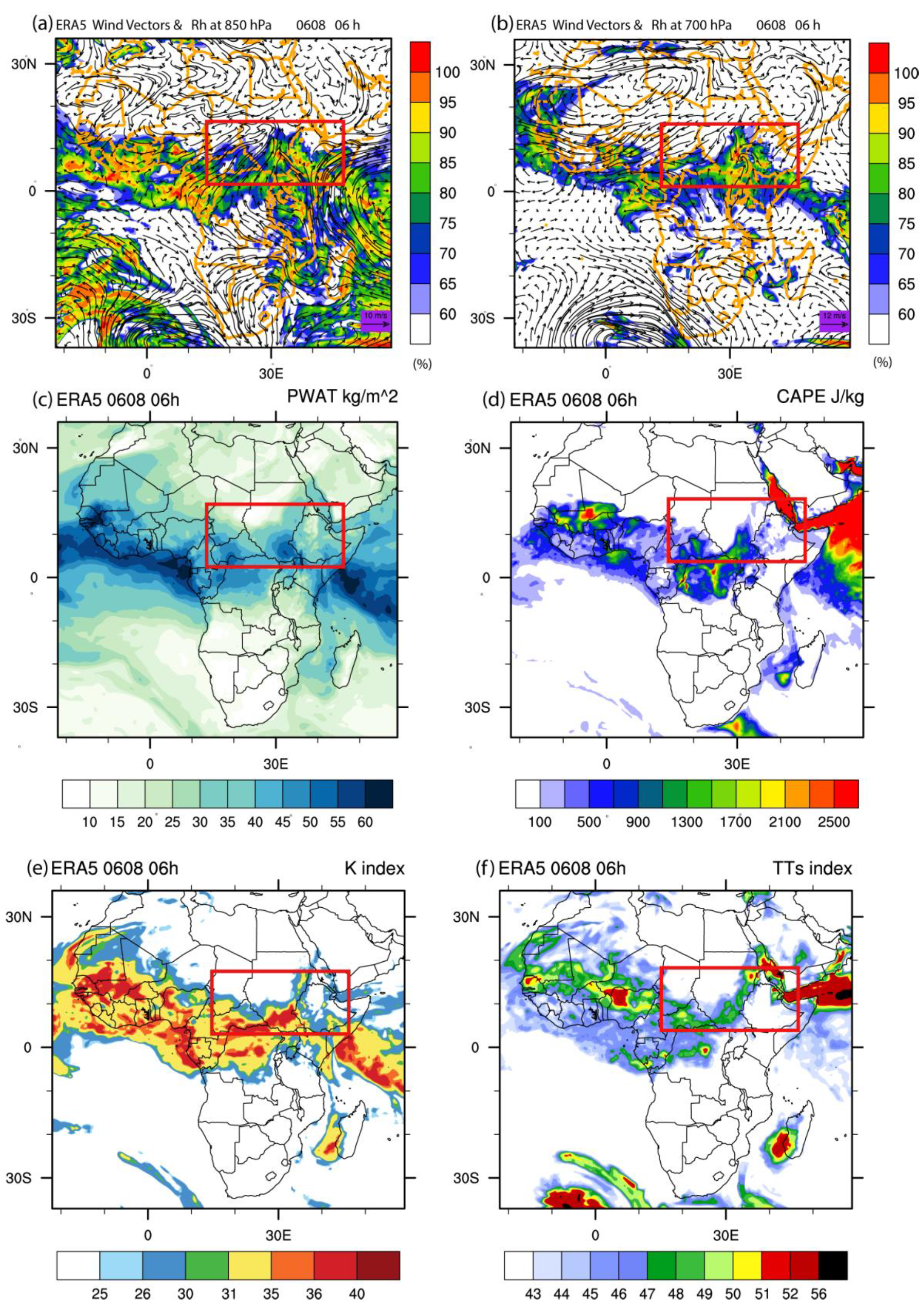
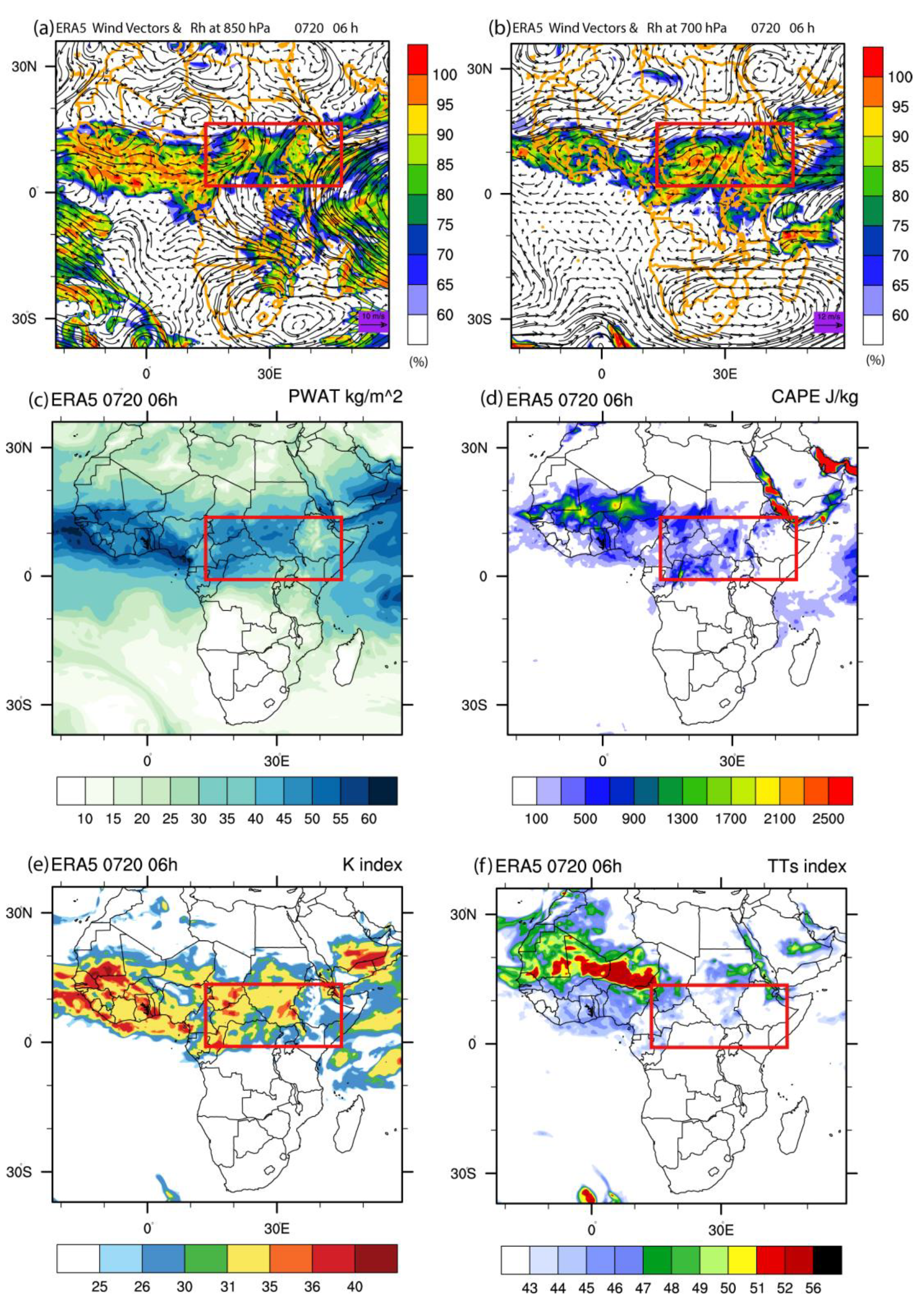
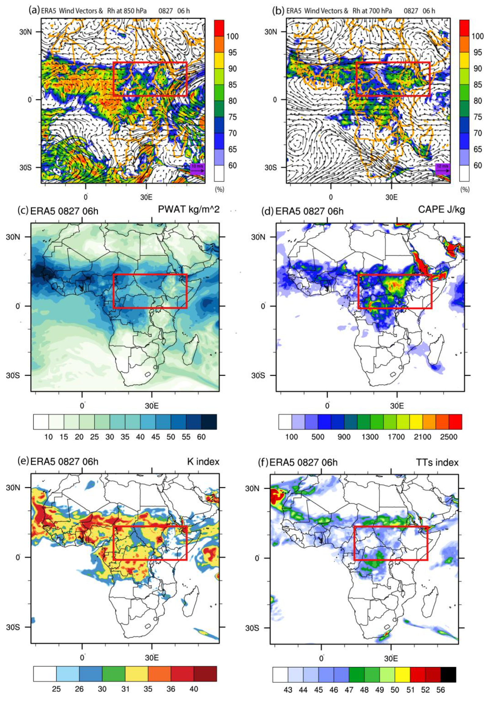
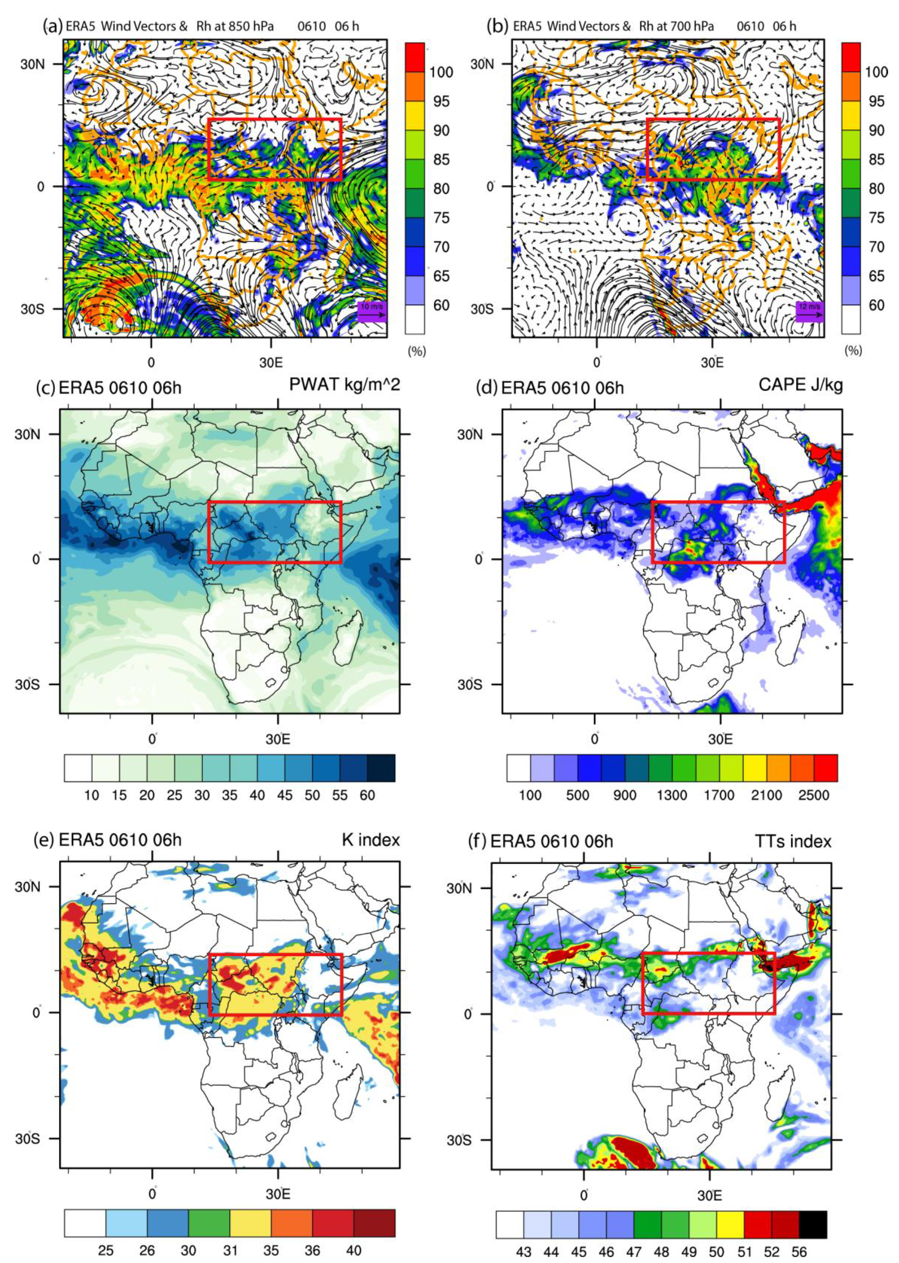
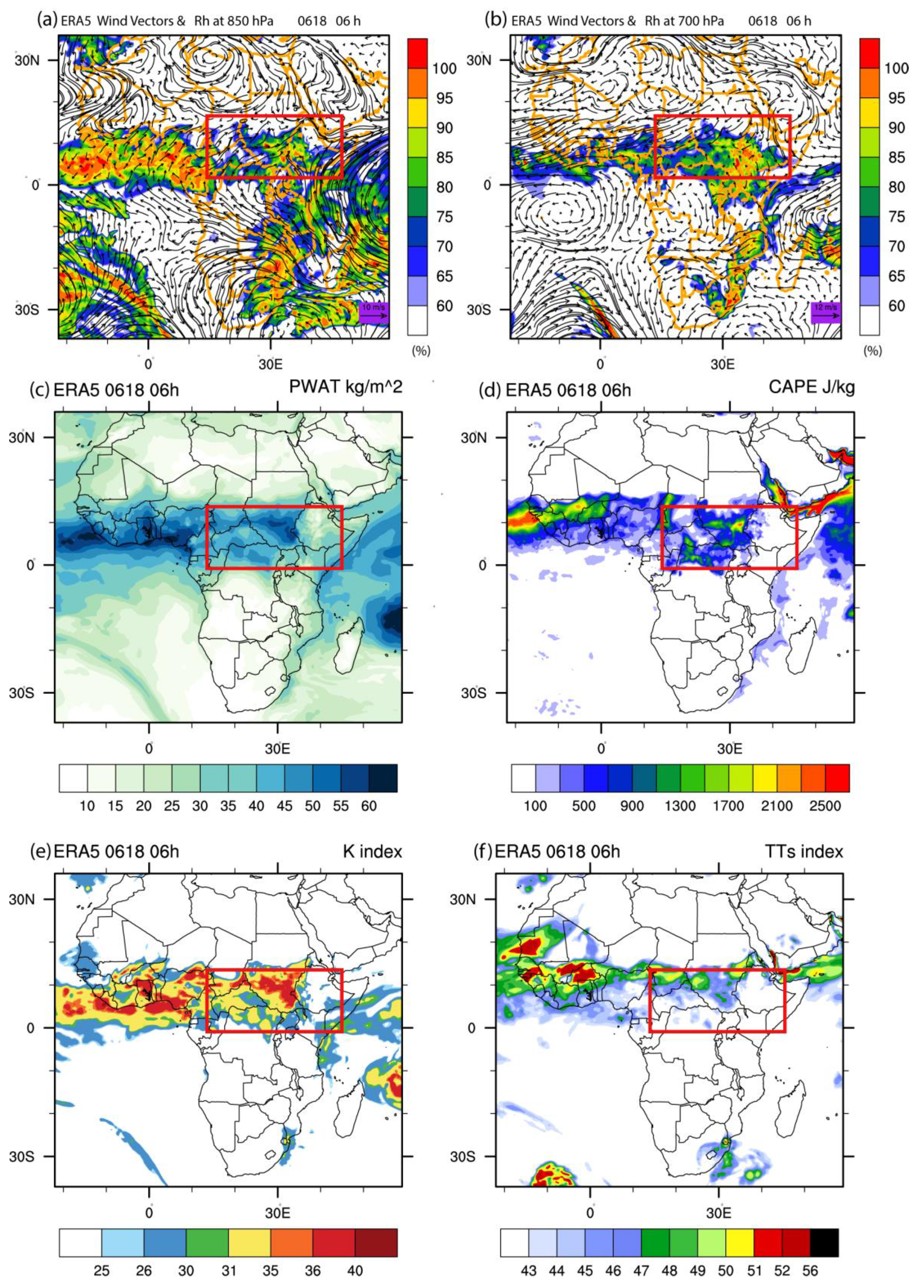
2.4. Synoptic Analysis of Severe Weather Events

Modelers and forecasters rely on atmospheric parameters to understand and discuss the favorable synoptic conditions and physical mechanisms accompanying heavy PRE events. Synoptic analyses serve as a practical way to predict convection activity. The present study used a quantitative evaluation method following [71]. Numerous studies have used these indices to reveal synoptic-scale features linked with heavy downpours [72,73]. A summary of the six key parameters used in the synoptic situation analysis is presented below.

2.4.1. Wind Circulation

To provide a synoptic view of the individual case events, we explored two key wind levels: (i) 850 hPa (to locate monsoon trough) and (ii) 700 hPa. This selection is consistent with past studies in East Africa and other regions [36,74].

2.4.2. Relative Humidity (RH)

RH is the ratio of vapor pressure ( e ) to saturation vapor pressure ( e s ). The amount of moisture in the atmosphere indicates the likelihood of PRE. RH is expressed mathematically [75] below:
e = Q P a 0.622
e s = 611 e x p ( 17.27 T a 237.3 + T a )
RH = e e s
where e is the vapor pressure, e s is the saturated vapor pressure, Q is the specific humidity, P a is the partial pressure (hPa), and T a is the atmospheric temperature (K).

2.4.3. Precipitable Water (PW)

PW reflects the amount of moisture in the atmosphere column and is a crucial indicator for heavy PRE prediction [76]. A higher PW value is associated with higher areal PRE coverage [77]. A PW of >20 kg/m−2 in the ROIs is generally associated with high downpours and vice versa. PW is expressed as follows:
PW = 1 g 0.622 . P w P 0.378 . P w dp
where g is gravity (9.81 m/s2), P w is the partial pressure of water vapor, dp is dew point temperature (K), and P is total atmospheric pressure (hPa).

2.4.4. Convective Available Potential Energy (CAPE)

CAPE is normally used to identify the atmospheric instability accompanying strong downpours. High CAPE values indicate greater instability (which indicates the potential for increased convection) and subsequent heavy PRE. CAPE < 495 J/kg is “weak instability”. CAPE of 1000–2500 J/kg is “moderate instability” and CAPE of >2500 J/kg indicates “strong instability” [71]. CAPE is expressed mathematically as follows:
CAPE = g Z LFC Z EL ( T vp T ve T ve ) dz
where g is gravity (9.81 m/s2), T vp is the virtual temp of the parcel, T ve is the virtual temperature of the environment, Z EL is the height of the equilibrium level, and Z LFC is the free convection level.

2.4.5. K-Index

The K-index measures thunderstorm potential. That is, it assesses the probability of a heavy storm [75]. Table S1 shows the threshold values for determining the operational significance of the K-index. High K-index values accompanied by high PW can lead to a rapid burst of intense PRE. The mathematical expression is shown below:
K = t 850 t 500 + t d 850 t 700 + t d 700
where t is temperature and t d is the dew point temperature.

2.4.6. Total of Totals Index (TTs)

The total of totals (TTs), following [73], was used as an indicator to assess the strength of heavy PRE. The threshold values shown in Table S2 categorize the potential strength of the heavy PRE events. TTs is expressed mathematically as follows:
TTs = t 850 + t d 850 2 t 500
where t and td denote air temperature and dew point temperature, respectively, and 850 and 500 represent the pressure levels (hPa).

3. Results

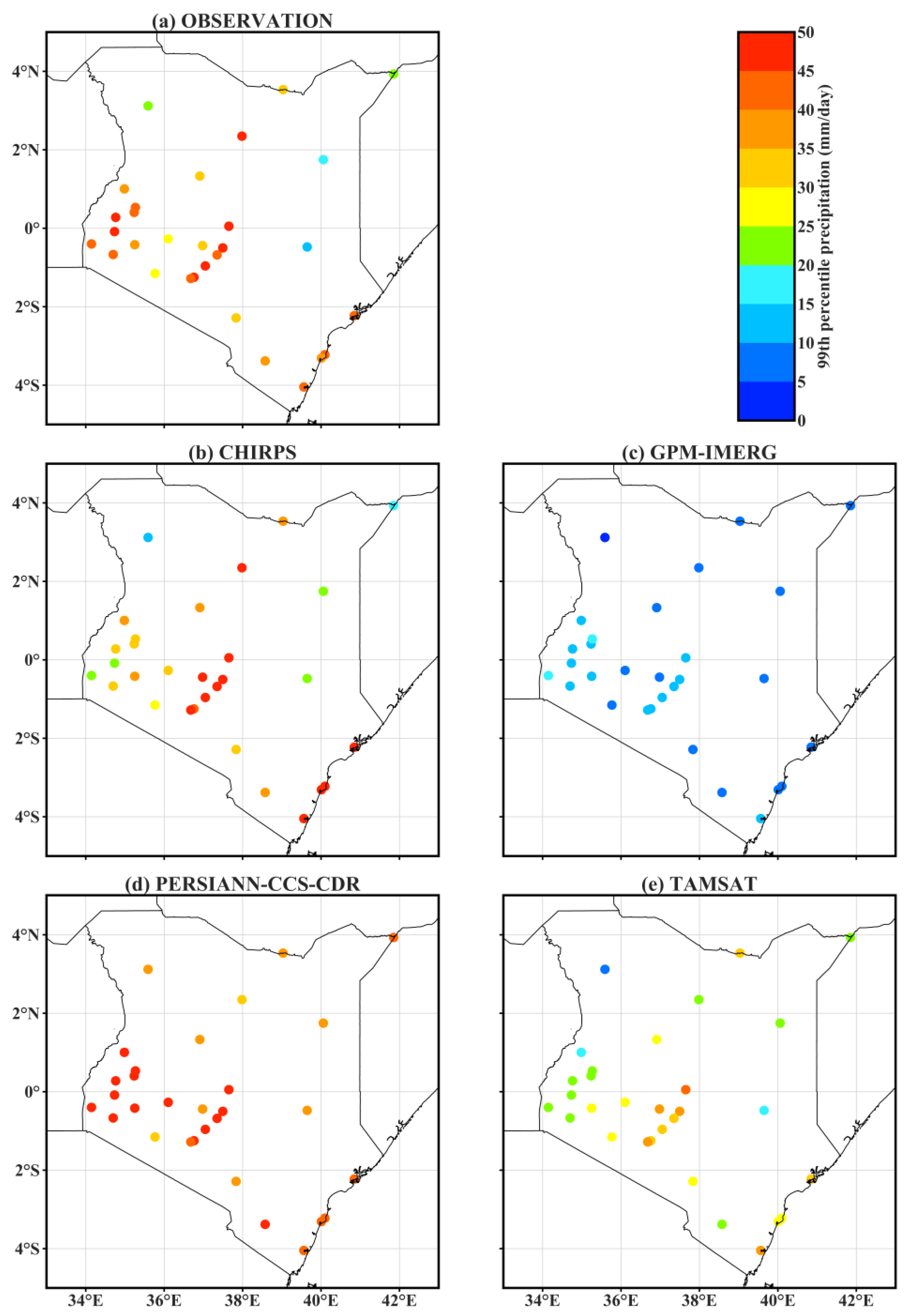
3.1. Spatial and Temporal Validation of Satellites PRE Datasets against Station Data

3.1.1. Mean Annual Cycle of PRE

To assess how the satellite data perform in reproducing the temporal variations, we analyzed the mean annual cycle over selected stations in Kenya. Figure S1 compares estimated monthly PRE annual cycles over Kenya at sampled stations by satellites and observations. Overall, the four satellite datasets captured the mean annual cycle pattern relative to the observed data throughout the year. However, the degree of estimation differed in wet and dry months. CHIRPS and PERSIANN-CCS-CDR overestimated PRE in wet months while TAMSAT overestimated PRE in dry months. GPM-IMERG products were underestimated in nearly all 30 stations used in Kenya. Generally, the temporal variations of the sampled stations showed that PRE varied from place to place. For example, many stations presented a bimodal PRE distribution (Figure S1) across the region in the overestimations of CHIRPS and PERSIANN-CCS-CDR.

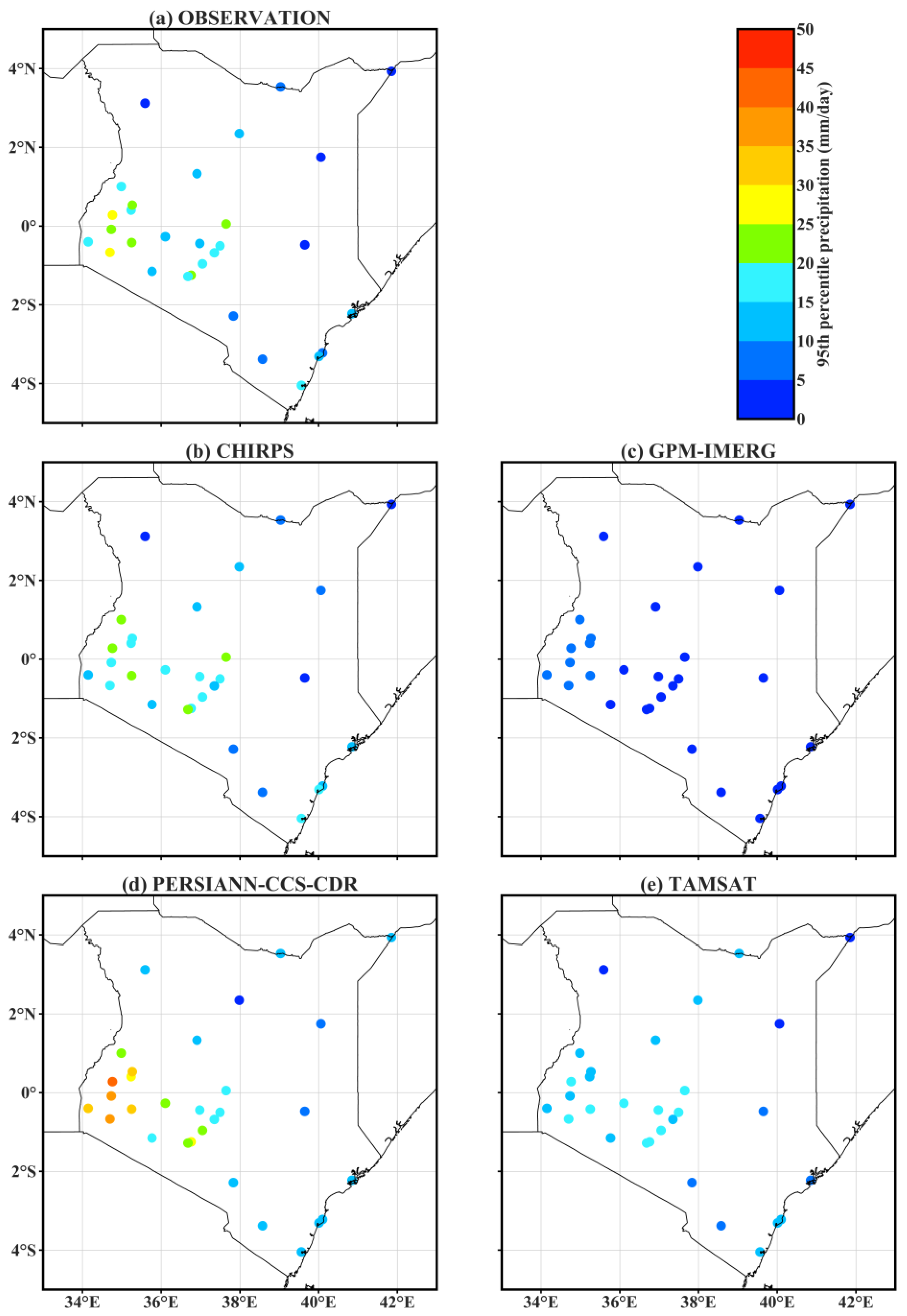
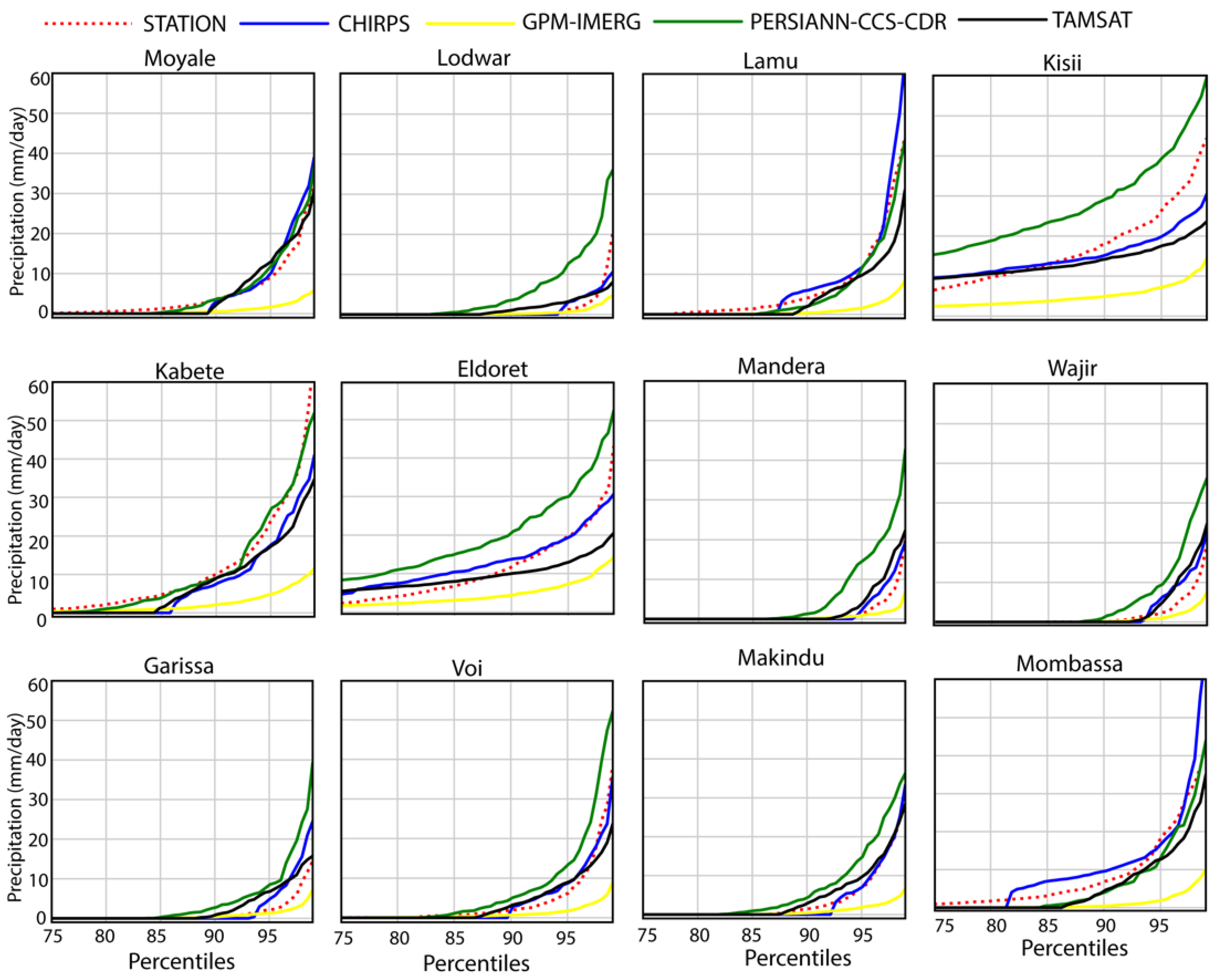
3.1.2. Performance of Satellite Data against Gauge Stations

To investigate the ability of the satellite datasets to replicate daily scale PRE extremes and to effectively capture their variations, we considered two standard percentile thresholds for extremes (i.e., the 95th and 99th percentiles—the results are presented in Figure 2 and Figure 3, respectively). Figure 2 and Figure S2 present the spatial distributions of observation and satellite estimates of 95th percentile rainfall quantities estimated from the 30 stations between 2013 and 2016 over Kenya.
Overall, the results revealed pronounced regional variations in the performance of the four satellite datasets. We observed larger differences in wet and mountainous regions compared with dry areas. Stations located in humid and mountainous regions in 34°–38°E and 2°S–2°N showed higher PRE values (29.03 mm/day) for the 95th percentile (Figure 2 and Figure S2) and 48.37 mm/day for the 99th percentile, respectively (Figure 3 and Figure S3). Non-humid and low-lying areas presented slightly lower values of <15 mm/day for the 95th and 99th percentile. Overall, PERSIANN-CCS-CDR and CHIRPS provided good spatial results for the extreme values that increased with the extreme threshold of 25 to 40 mm/day. Similar results were shown in rainfall events exceeding 20 mm/day (R20 mm in Figure S4). The differences may be explained by the retrieval algorithms or sensors used to estimate PRE. PERSIANN-CCS-CDR and CHIRPS performed better than TAMSAT and GPM-IMERG. PERSIANN-CCS-CDR data are based on passive and active microwave observations and CHIRPS is based on infrared cold cloud detection. The difference in their performance may be related to the retrieval algorithms or the type of data source used.
To assess the suitability of the four satellite products to detect extreme PRE, we compared the standard percentile thresholds for extremes (i.e., from the 75th percentile and above) against the observed data. Figure 4 illustrates the performances of the four satellite data at the 75th, 95th, and 99th percentile values against gauge stations. The accumulated daily PRE from the sampled stations during the 2013–2016 period were categorized into quartiles to evaluate the accuracy of the satellite data relative to the observed data (Figure 4). During the period 2013–2016, values of >10 mm/day and >20 mm/day for the 95th and 99th percentiles were consistent and comparable across all stations for CHIRPS (blue color) and PERSIANN-CCS-CDR (green color). Overall, the daily PRE of CHIRPS (blue color) and PERSIANN-CCS-CDR (green color) were close to the observed station PRE before the 90th percentile. However, they overestimated above the 95th percentile (Figure 4). Similar results are shown for GPM-IMERG (yellow color) and TAMSAT (black color), but they tended to underestimate the data (Figure 5). The exceptions to the above patterns included stations such as Kissi and Eldoret (Figure 4), where PERSIANN-CCS-CDR overestimated between the 75th and 99th percentile.
In summary, this study selected PERSIANN-CCS-CDR as the closest reference dataset based on validation with respect to rain gauge observations.

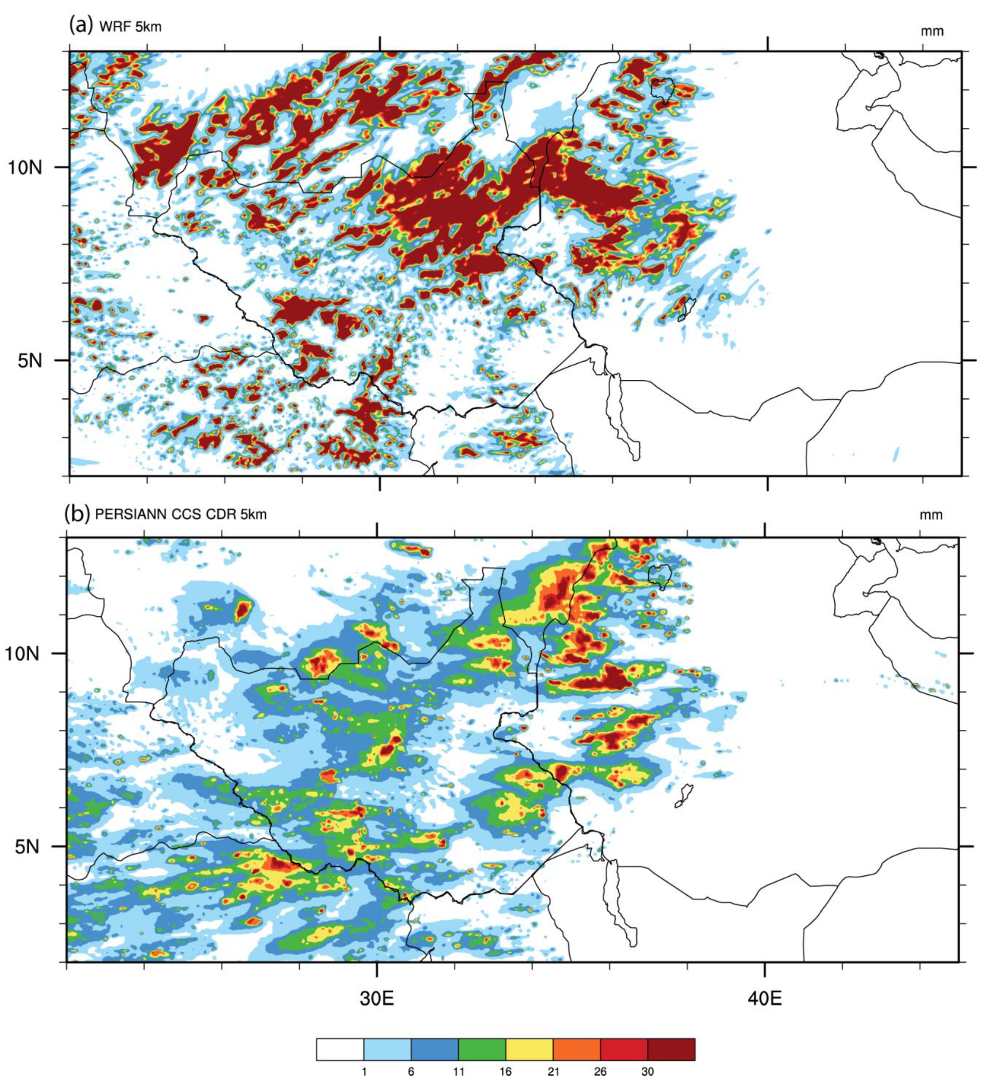
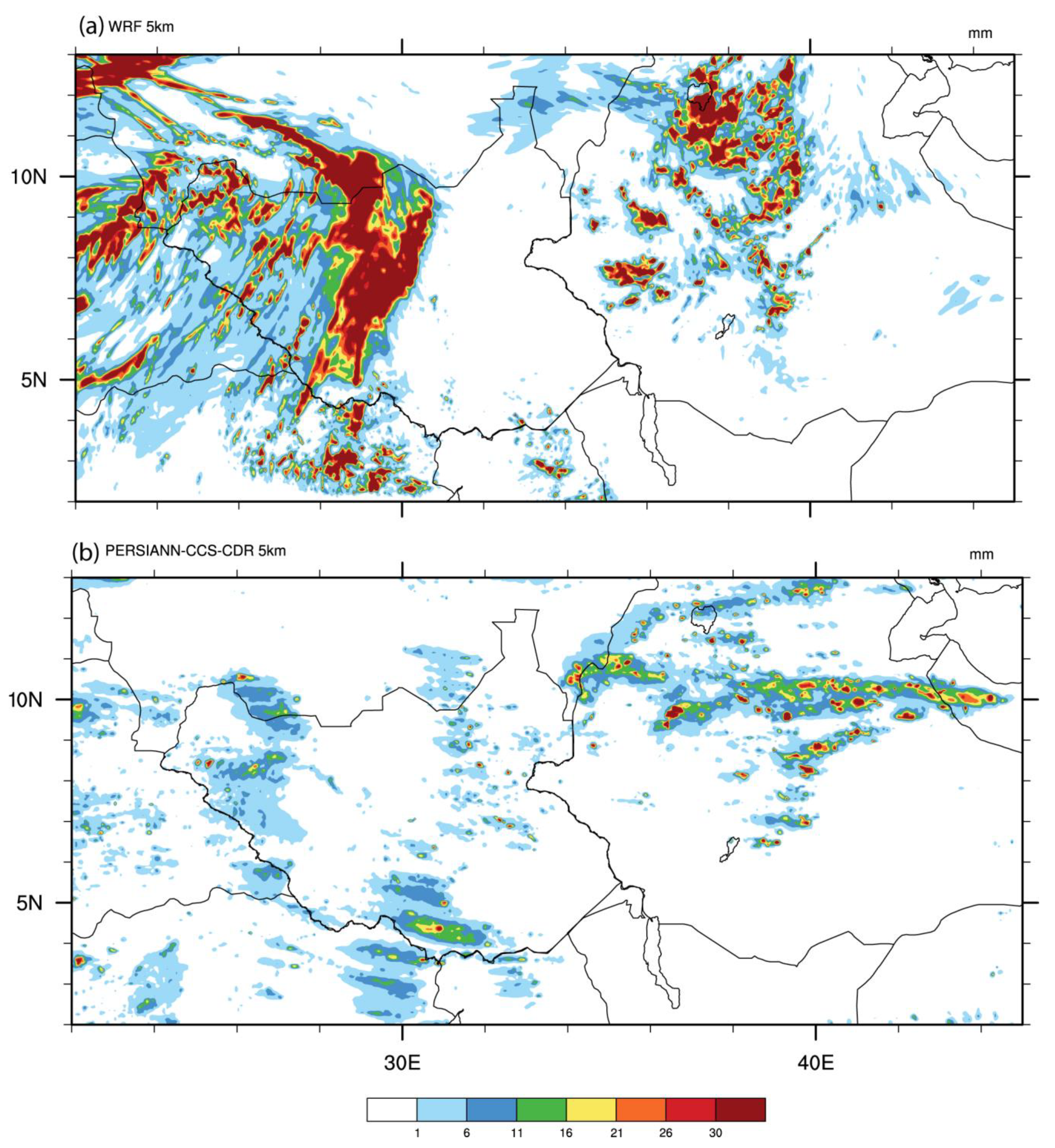
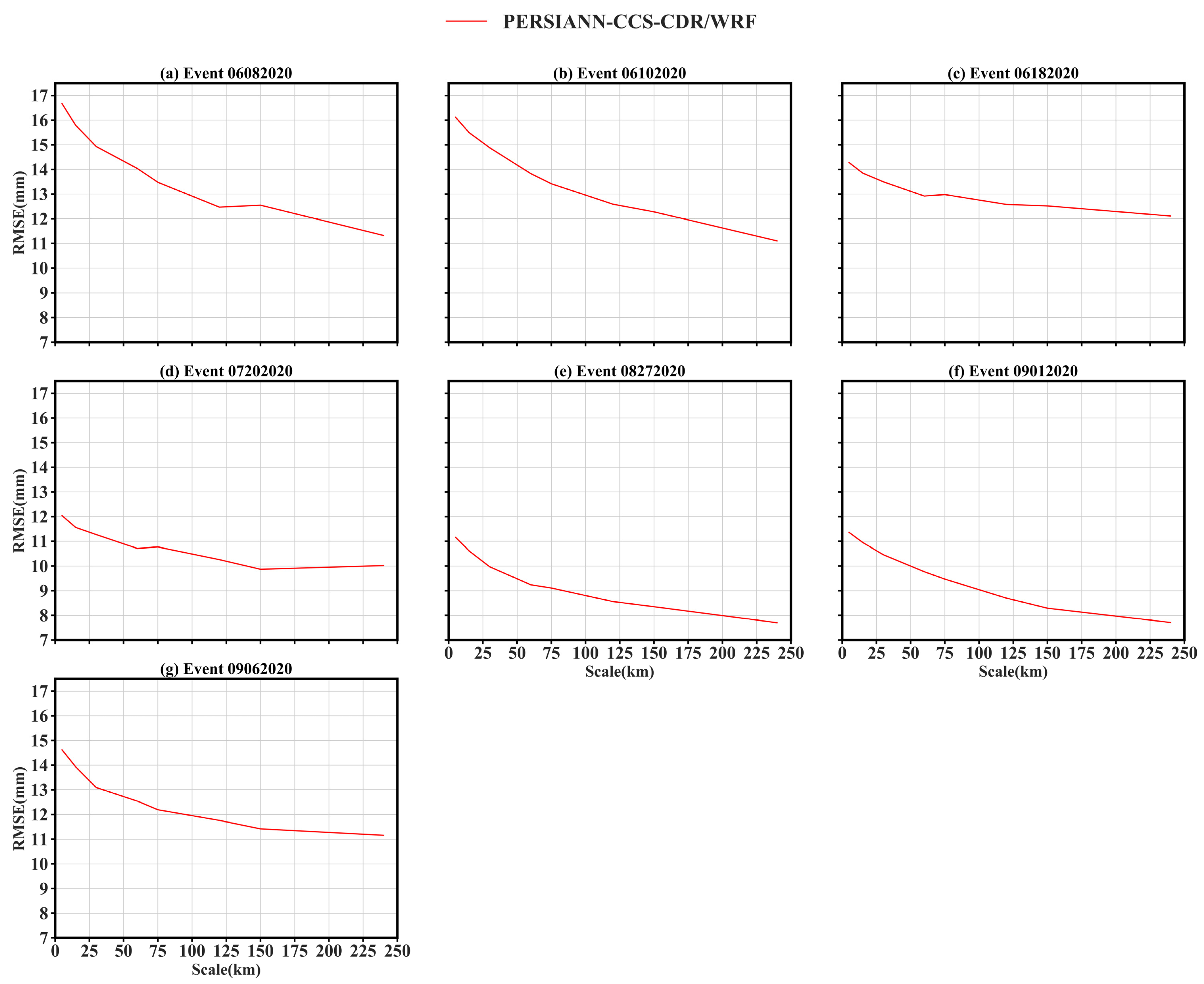
3.2. Comparison of Heavy PRE from WRF and Satellite Estimates

In this section, we examine the capability of WRF to accurately simulate the heavy PRE events (Table 1) that wreaked havoc on lives and property in the summer of 2020. The WRF outputs were evaluated against one high-resolution satellite’s PRE products (i.e., PERSIANN-CCS-CDR) to infer the satellite and model relative potential to capture the location and intensity of PRE during the case studies and to provide more details on the individual events as reported in the media [2,3]. The choice of PERSIANN-CCS-CDR as the reference satellite dataset was based on validation with respect to the rain gauge observations. The satellite estimates and simulated PRE were based on a 24 h accumulated PRE. Figure 5, Figure 6, Figure 7, Figure 8 and Figure 9 show the spatial distribution of the simulated and observed PRE over East Africa. Similar results in Figures S5 and S6 present heavy PRE events recorded on 1 and 6 September 2020, respectively.

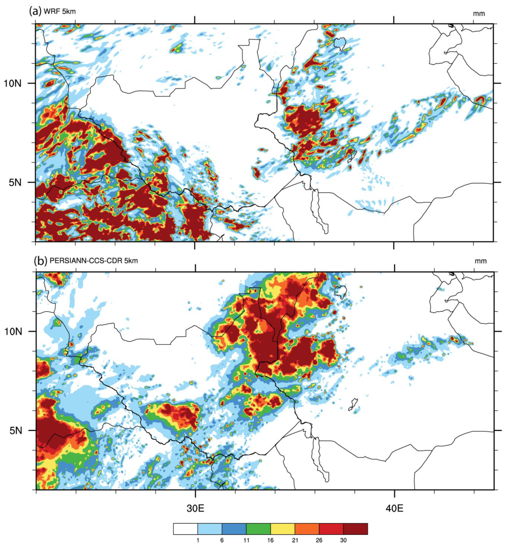
3.2.1. Case 1 (8 June 2020)

On 8 June 2020, heavy PRE along the South Sudan (SS)–Ethiopia (ET) border region caused devastating flash flooding [2,3]. Figure 5 shows the spatial pattern of simulated and observed PRE on that day.
The WRF model reproduced the PRE spatial distribution in the ROI well compared to satellite products (Figure 5a). The PRE event was also satisfactorily estimated in the PERSIANN-CCS-CDR data (Figure 2b) but with distinct patterns and intensities (WRF: 26–30 mm/day; PERSIANN-CCS-CDR: 21–30 mm/day).

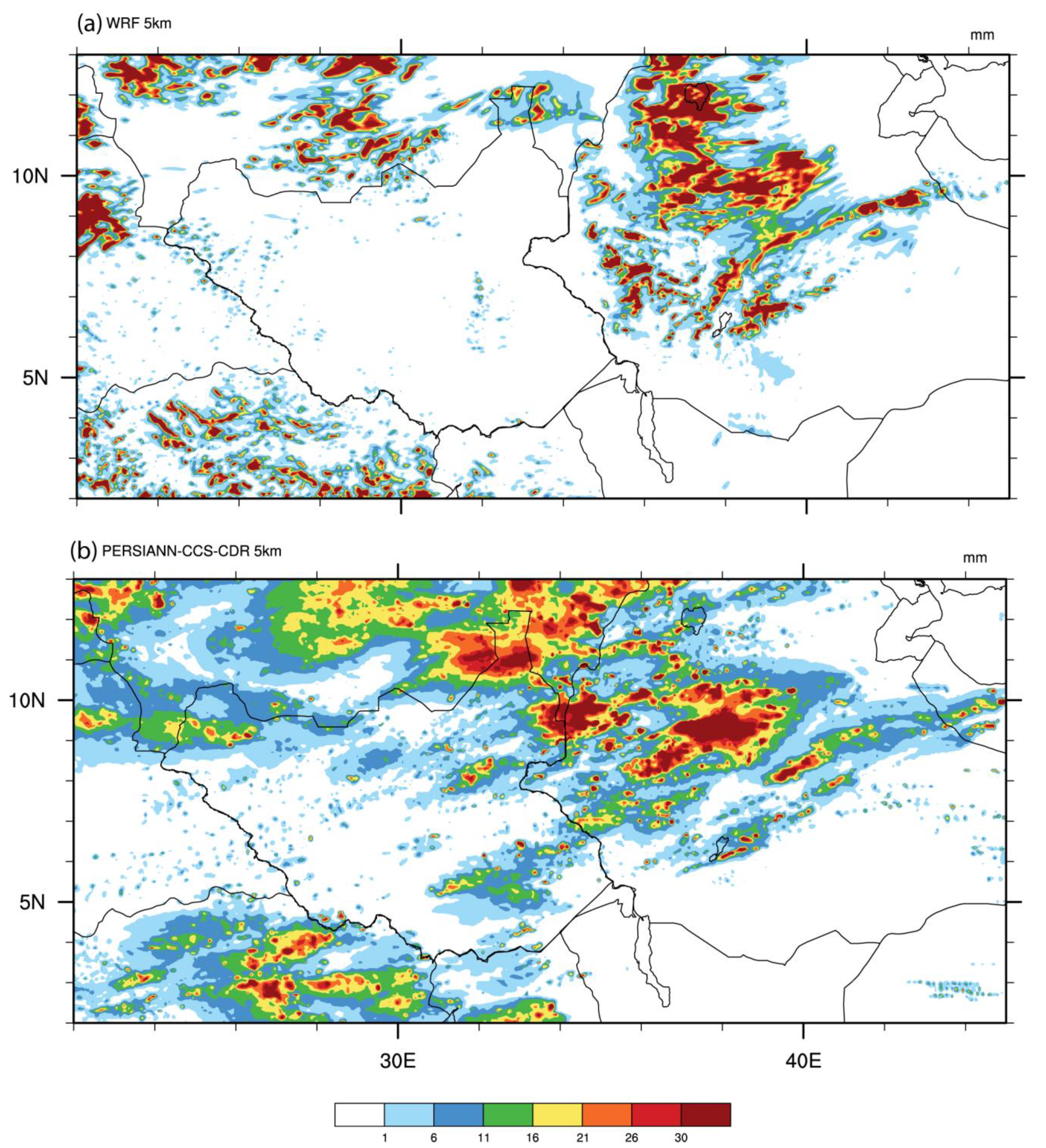
3.2.2. Case 2 (10 June 2020)

Two days later, on 10 June 2020, another heavy PRE event occurred along the SS–ET border. The media reported that this event destroyed school buildings, health facilities, roads, and farmlands in South Sudan [2,3]. The results are illustrated in Figure 6. Comparing the WRF output (Figure 6a) with the satellite data (Figure 6), the model reproduced this PRE event well. We observed several similarities between the PERSIANN-CCS-CDR (Figure 6b) and WRF PRE magnitude estimates. The PRE distribution from PERSIANN-CCS-CDR (Figure 6b) exhibited a similar spatial pattern, but the spatial spread was more pronounced than the WRF outputs.
Figure 6. Distribution of simulated and observed precipitation (mm/day) on 10 June 2020 over East Africa. (a) WRF; (b) PERSIANN-CCS-CDR.
Remotesensing 14 01964 g006

3.2.3. Case 3 (18 June 2020)

On 18 June 2020, a heavy storm occurred again in the same ROI (Figure 7). According to the media reports, this event aggravated relief efforts for the previous event (Case 2) by aid agencies as road infrastructure was still unavailable [2,3]. The spatial pattern of simulated PRE shows that WRF (Figure 7a) reproduced the PRE event well, as was captured by the PERSIANN-CCS-CDR (Figure 7b). In brief, the results for Case 3 showed that the WRF model captured this heavy PRE event with estimates of >30 mm/day. The PERSIANN-CCS-CDR satellite product captured the event in terms of spatial patterns but with PRE magnitudes of 11–30 mm/day.
Figure 7. Distribution of simulated and observed precipitation (mm/day) on 18 June 2020 over East Africa. (a) WRF; (b) PERSIANN-CCS-CDR.
Remotesensing 14 01964 g007

3.2.4. Case 4 (20 July 2020)

The heavy PRE on 20 July 2020 caused extensive flooding, displacing 300,000 people and destroying about 5000 homes [2,3]. We compared the spatial pattern and PRE magnitudes from WRF and PERSIANN-CCS-CDR (Figure 8). The WRF model captured this heavy PRE event in the interior of Ethiopia.
The simulated PRE magnitude was >30 mm/day (Figure 8a). PERSIANN-CCS-CDR (Figure 8b) showed values of 11–26 mm/day and patches of >30 mm/day. Overall, the spatial patterns of the WRF output and PERSIANN-CCS-CDR were comparable but with major differences in the PRE estimates.
Figure 8. Distribution of simulated and observed precipitation (mm/day) on 20 July 2020 over East Africa. (a) WRF; (b) PERSIANN-CCS-CDR.
Remotesensing 14 01964 g008

3.2.5. Case 5 (27 August 2020)

On 27 August 2020, heavy PRE occurred in Sudan, Uganda, and Kenya [2,3]. In Sudan, 381,770 people were affected and 84 died. In total, 37,000 homes were destroyed, and 34 schools and 2671 health facilities were damaged. In Uganda, 8700 people were displaced, one person died, and 800 homes were destroyed. In Kenya, 1000 families were displaced in the Lake Turkana region (northwestern Kenya) [2,3]. The PRE spatial pattern of this event is displayed in Figure 9. The ROI for this case included Sudan, South Sudan, Ethiopia, Uganda, and Kenya.
Figure 9. Distribution of simulated and observed precipitation (mm/day) on 27 August 2020 over East Africa. (a) WRF; (b) PERSIANN-CCS-CDR.
Remotesensing 14 01964 g009
The spatial pattern of the WRF output (Figure 9a) and the PERSIANN-CCS-CDR product (Figure 9) were comparable over Sudan, South Sudan, and Ethiopia. The spatial pattern and magnitude of PERSIANN-CCS-CDR (Figure 9b) were comparable to the WRF results. In particular, the WRF results were closer to the PERSIANN-CCS-CDR results over Ethiopia and Sudan, but the event was poorly reproduced over South Sudan, Uganda, and Kenya. The WRF output PRE magnitudes (>1 mm/day) were comparable to those of PERSIANN-CCS-CDR (Figure 5b).
In summary, the WRF model output exceeded the observed PRE data most of the time. The reasons for this overestimation are unclear and are beyond the scope of this study. However, some factors that may influence WRF’s overestimation of the PRE include the numerical scheme used or the microphysics and planetary boundary layer schemes, which are consistent with past studies [14,77].
Overall, the WRF model reproduced the spatial pattern of the seven heavy PRE events well. Additionally, the spatial pattern of the heavy PRE was captured by the PERSIANN-CCS-CDR products (Figure 5, Figure 6, Figure 7, Figure 8 and Figure 9, Figure S6 and S7).
We further investigated which scale was appropriate for capturing the PRE intensities. The WRF outputs were compared to those of PERSIANN-CCS-CDR based on the area-related root mean square error (RMSE) following Rezacova et al. [50]. The averaged area-related RMSE for each event was computed and plotted against the spatial scale (Figure 10). From these results, the RMSE variability was scale-dependent. Overall, the result indicated that as the peak PRE intensity in the model was displaced with respect to the observed, the RMSE tended to decrease at larger spatial scales. This provides additional value for weather forecasters and researchers to assess the applicability of WRF in operational forecasting or warning systems.

3.3. Synoptic Conditions during Heavy PRE Events

We examined the wind circulation and RH flow patterns at 6 a.m. on the 8th, 10th, and 18th of June; 20th of July; and 27th of August 2020. Figure 11a–d, Figure 12a–d, Figure 13a–d, Figure 14a–d and Figure 15a–d present the spatial distribution of the major observed features from ERA5. Wind and humidity are among the main parameters forecasters use to predict the likelihood areas of deep convective activity initiation [26]. Figure 11a–d, Figure 12a–d, Figure 13a–d, Figure 14a–d and Figure 15a–d present several major characteristics during the heavy PRE cases.
Figure 11. Synoptic analysis of ERA5 data at 6am (UTC) on 8 June 2020. (a) wind at 10 m (m/s; vectors) and relative humidity (%; shaded) at 850 hPa; (b) wind (m/s; vectors) and relative humidity (%, shaded) at 700 hPa; (c) precipitable water (kg/m2); (d) convective available potential energy (J/kg); (e) K-index; and (f) total of totals index. The red box denotes the ROI (South Sudan–Ethiopia border).
Remotesensing 14 01964 g011
In Case 1, the ERA5 data reasonably estimated strong (10 m/s) westerly winds at 850 hPa over the entire 5–15°N area. A cyclonic circulation over the Guinea Coast and a north (northeasterly) wind prevailed over the region (Figure 11a, Figure 12a, Figure 13a, Figure 14a and Figure 15a). However, there was high anticyclonic activity over the Southern Hemisphere in the Atlantic and Indian Oceans (Figure 11a, Figure 12a, Figure 13a, Figure 14a and Figure 15a), resulting in stronger cold advection over the range of 5–15°N (Figure 11a, Figure 12a, Figure 13a, Figure 14a and Figure 15a). Figure 11a, Figure 12a and Figure 13a (% shaded) present nearly 75% of RH in the equatorial region (red box) at 850 hPa. Figure 11a, Figure 12a, Figure 13a, Figure 14a and Figure 15a present a circulation pattern at 850 hPa characterized by a monsoon trough (i.e., the flow convergence with high RH values of >80% was for identifying of vortices). The anticyclonic circulations over the Indian Ocean and westerly (southwesterly) winds prevailing over the range of 5–15°N illustrate a relatively shallow trough (Figure 11a, Figure 12a, Figure 13a, Figure 14a and Figure 15a). Figure 11b, Figure 12b, Figure 13b, Figure 14b and Figure 15b present 70–80% of RH in the ranges 5–10°N and 25–35°E (red box). These features are consistent with the region’s climate and an important indicator for the development of convection. The observed maximum speed was 10–16 m/s over the ranges of 25–35°E and 10–15°N (Figure 11b, Figure 12b, Figure 13b, Figure 14b and Figure 15b). The strong cyclonic circulation over the entire 10–15°N area was well captured in ERA5. We confirmed from the atmospheric instability indices that the conditions were favorable for convective activities (PW > 20 kg/m2; CAPE > 750 J/kg; K-index > 35 °C; and TTs < 47; Figure 11c–f, Figure 12c–f, Figure 13c–f, Figure 14c–f and Figure 15c–f), which is consistent with the guidelines in [71].
Similarly, in other case events, we observed that the wind and RH fields simulated by ERA5 were southwesterly winds (Figure 11a, Figure 12a and Figure 13a), transporting moist air from the Atlantic Ocean into the equatorial region (Figure 11a,b, Figure 12a,b, Figure 13a,b, Figure 14a,b and Figure 15a,b). In Case 2, the event was identified as a cyclonic event at 700–850 hPa, in addition to the monsoon flow (Figure 12a,b), with RH > 85%. The physical mechanism prevailing on this day (06:00) was consistent with [71] conditions for heavy downpours; high PW (Figure 12c, >55 kg/m2), moderate CAPE values (Figure 12d, >1300 kg/m2), high K-index (Figure 12e, >35 °C), and high TTs (Figure 12f, >45).
Figure 12. Synoptic analysis of ERA5 data at 6am (UTC) on 10 June 2020. (a) wind at 10 m (m/s; vectors) and relative humidity (%; shaded) at 850 hPa; (b) wind (m/s; vectors) and relative humidity (%, shaded) at 700 hPa; (c) precipitable water (kg/m2); (d) convective available potential energy (J/kg); (e) K-index; and (f) total of totals index. The red box denotes the ROI (South Sudan–Ethiopia border).
Remotesensing 14 01964 g012
In Case 3, the synoptic conditions on this day over the range 25–35°E and 5–10°N (red box) showed unique characteristics. A PW of >45 kg/m2 (40–50 kg/m2; Figure 13c), high CAPE values of >2100 J/kg (reaching a maximum of 2500 J/kg; Figure 13d), a K-index of >36 c (31–40 °C; Figure 13e), and TTs values of >49 (48–51; Figure 13f) were consistent with a heavy downpour.
Figure 13. Synoptic analysis of ERA5 data at 6am (UTC) on 18 June 2020. (a) wind at 10 m (m/s; vectors) and relative humidity (%; shaded) at 850 hPa; (b) wind (m/s; vectors) and relative humidity (%, shaded) at 700 hPa; (c) precipitable water (kg/m2); (d) convective available potential energy (J/kg); (e) K-index; and (f) total of totals index. The red box denotes the ROI (South Sudan–Ethiopia border).
Remotesensing 14 01964 g013
The synoptic analysis (Figure 14a,b) and atmospheric instability as presented in Case 4 provided evidence for convective activity; high PW of >20 kg/m2 (Figure 14c), CAPE of <750 J/kg (Figure 14d), K-index of >35 °C (Figure 14e), and TTs of <45 (Figure 14f).
Figure 14. Synoptic analysis of ERA5 data at 6am (UTC) on 20 June 2020. (a) wind at 10 m (m/s; vectors) and relative humidity (%; shaded) at 850 hPa; (b) wind (m/s; vectors) and relative humidity (%, shaded) at 700 hPa; (c) precipitable water (kg/m2); (d) convective available potential energy (J/kg); (e) K-index; and (f) total of totals index. The red box denotes the ROI (South Sudan–Ethiopia border).
Remotesensing 14 01964 g014
Lastly, Case 5 revealed that the atmospheric instability (PW > 45 mm, CAPE < 900 J/kg; K-index > 35 °C and TTs < 45 (Figure 15c–f, red box)) was favorable for convective activity on 27 August 2020 and this is consistent with the guidelines for heavy downpours [71]. Additionally, this result is consistent with the climatological behavior of the region as described by Nicholson [78,79,80].
Figure 15. Synoptic analysis of ERA5 data at 6 a.m. (UTC) on 27 June 2020. (a) wind at 10 m (m/s; vectors) and relative humidity (%; shaded) at 850 hPa; (b) wind (m/s; vectors) and relative humidity (%, shaded) at 700 hPa; (c) precipitable water (kg/m2); (d) convective available potential energy (J/kg); (e) K-index; and (f) total of totals index. The red box denotes the ROI (Sudan, South Sudan, Ethiopia, Uganda, and northwestern Kenya).
Remotesensing 14 01964 g015

4. Discussions

East Africa is a flood-prone region, and frequent flash flooding is a major disaster. In 2020, multiple heavy PRE events caused by summer convective activities destroyed infrastructure in the region, displaced thousands, and killed many [2,3]. In this study, we selected seven case events using the database from EM-DAT and floodlist websites (Table 1). Two main objectives were explored: (a) to investigate the capability of the WRF to simulate the heavy PRE events, and (b) to understand the synoptic conditions accompanying the summer 2020 heavy PRE events. The WRF model was used to simulate the heavy PRE events reported in these reliable databases [2,3]. The WRF experiments were configured over three nested domains.
The reliability of satellite products depends on the region considered [25]. This study investigated the spatio-temporal performance of four high-resolution satellite datasets against gauge stations. Since the focus of this study was on flash floods, we based the verification study on standard percentile thresholds for extremes following [48] and defined extreme PRE as daily PRE exceeding the 95th and 99th percentiles. Note that the objective of this part was the verification of the best-performing data for the study region(s) due to the four satellites’ differences in spatial and temporal resolutions.
Overall, the results revealed pronounced regional variations in the performance of the four satellite data. We observed larger differences in wet and mountainous regions than in dry areas. Overall, PERSIANN-CCS-CDR provided good spatial results for the extreme values that increased with an increasing extreme threshold of >25–40 mm/day. GPM-IMERG products were underestimated in nearly all 30 stations used in Kenya. This result is interesting as this product performed well in East Africa according to Le Coz’ [25] review. Reasons such as the number and location of the rain gauges, the season, the region, and the evaluation statistics used may partly explain this phenomenon. Other reasons may be related to the differences in the retrieval algorithms or sensors used to estimate PRE [24,25]. These evaluation results showed that PERSIANN-CCS-CDR was closer to the gauge data than the rest, especially for the extreme events. This finding was not surprising as PERSIANN-CCS-CDR is designed for heavy PRE events [27]. Thus, we selected these satellites to assess against the WRF model. The objective here was not to confirm the superiority of any satellite datasets (PERSIANN-CCS-CDR, GPM IMERG, CHIRPS, or TAMSAT), but rather to demonstrate their potential utilization in a local context, particularly for heavy PRE in East Africa.
We compared the WRF output against high-resolution PERSIANN-CCS-CDR products to infer their relative potential to capture heavy PRE events (Table 1). Satellite-based estimates serve as an indirect measure of PRE and are useful in regions with a low density of weather station networks. Additionally, satellite PRE products have the advantage of high spatial coverage. We focused on reported case events in East Africa. The WRF model reproduced the heavy PRE events well (Figure 5a, Figure 6a, Figure 7a, Figure 8a and Figure 9a, Figures S5 and S6a). The simulated heavy PRE in Sudan and South Sudan, extending to some parts of northwestern Ethiopia, eastern Kenya, and northwestern Uganda, are common from June to September. Similar results were reported in Nicholson [41]. Overall, the results are consistent with previous studies that used WRF for other case events [81,82]. Our results are consistent with Li et al.’s [8] assertion that five African countries prone to floods are located in East Africa. The magnitude of the simulated PRE was then analyzed. The PRE magnitudes varied between individual events. The distinct spatial patterns showed the WRF model simulated > 30 mm/day in all case events except for the 27 August event (Case 5), which was poorly reproduced over Uganda and Kenya. Overall, the magnitude of PRE is somewhat consistent with Kimambo et al. [82] for the region. These findings indicated that, in a local context, the WRF model shows good performance in simulating spatial patterns and PRE magnitudes. Hence, the WRF model can be a useful and valuable tool for sub-seasonal processes. We found that its applications could improve local and short-term forecasting, which is consistent with the literature [11,81]. Similarly, the WRF PRE magnitudes were noticeably closer to the PERSIANN-CCS-CDR PRE estimates and are consistent with Kimambo et al. [82]. The practical implication of these findings is that PERSIANN-CCS-CDR presents a better potential for sub-seasonal applications over East Africa.
From a meteorological perspective, heavy PRE events may be accompanied by large-scale synoptic systems. The synoptic situation on a given day is complex and determined by a combination of factors [83]. ERA 5 reanalysis was used to verify the large-scale circulation pattern, relative humidity fields, and other atmospheric instability patterns accompanying the heavy PRE. The synoptic patterns accompanying the events on the 8th, 10th, and 18th of June, 20th of July, and 27th of August were analyzed (Figure 11, Figure 12, Figure 13, Figure 14 and Figure 15). The physical mechanisms accompanying the summer 2020 heavy PRE events were examined. The wind and relative humidity were analyzed and the results are illustrated in Figure 11, Figure 12, Figure 13, Figure 14 and Figure 15. Generally, the wind circulation and relative humidity climatology were a regime of large westerlies (southwesterlies) that transported moist air (RH) from the Atlantic Ocean into Africa, while northerlies and northeasterlies mostly formed the cyclones in the north. The two converged in the range of 5–15°N to form a monsoon trough. This is in agreement with [84]. We observed that individual cases showed distinct RH values. However, the values were all >70% (Figure 11, Figure 12, Figure 13, Figure 14 and Figure 15, % shaded). Generally, the event was identified as a cyclonic event at 850 hPa and the monsoon flow (Figure 11a), with RH >75% due to low-level moisture convergence, was a good indicator of convection. Our results are in line with [81,82,84]. We further analyzed other parameters to understand atmospheric instability prior to these events. We selected PW, CAPE, K-index, and TTs to examine whether they provided conditions favorable for convective activities. Overall, different case events presented distinct patterns of synoptic conditions. Figure 11, Figure 12, Figure 13, Figure 14 and Figure 15 suggest favorable conditions for a heavy downpour. The wind circulation and moisture flow pattern over the ROI were characterized by flow convergence that mirrored the climatological behavior of the region. These findings are consistent with Kimambo et al. [82]. In other regions, these parameters have been used as good convection indicators. Similarly, the atmospheric instabilities indices (PW, CAPE, K-index, and TTs) were confirmed as good indicators of heavy PRE in the ROI and adjoining regions. The evidence of strong convective activity is consistent with the guidelines in [71].
From an early warning system perspective, this study provided vital climate and weather information that may help formulate preventive measures. This information is useful to forecasters because it provides case studies of severe weather. From the perspective of Earth observation scientists, space has untapped potential. The use of satellites to tackle the threats and challenges faced by humanity makes a big difference in the ongoing climate change debate. As satellites watch over Earth continuously, the recorded data can help us monitor, understand, model, and predict climate change and its related challenges. Further research on other case events would improve our confidence in adopting this type of analysis in developing countries where budget allocation for research is limited.

5. Conclusions

We demonstrated the location and extent of the summer 2020 heavy PRE in East Africa by (1) carrying out a verification process that selected the best-performing satellite data over the region, (2) using satellite(s) data to evaluate the WRF simulation of seven case events that occurred in East Africa, and (3) examining the pattern of synoptic conditions prior to these events. Based on our findings, the following conclusions were drawn:
Based on the performance of the four individual high-resolution satellites against gauge stations, PERSIANN-CCS-CDR performed better in the 75th, 95th, and 99th percentile.
The PERSIANN-CCS-CDR product captured the spatial pattern of all case events in the region despite distinct differences in PRE distribution and magnitudes. The spatial pattern of the WRF output was close to that of PERSIANN-CCS-CDR in all the cases, with the area-related RMSE decreasing obtained with increasing scale for all the events.
Further analysis of other parameters to understand atmospheric instability prior to these events presented a distinct pattern of synoptic conditions. The results suggest that the wind circulation and moisture flow pattern over the ROI were characterized by a flow convergence that mirrored the climatological behavior of the region. The atmospheric instability indices (PW, CAPE, K-index, and TTs) were confirmed as good indicators of the heavy PRE that occurred in the summer of 2020 in East Africa.

Supplementary Materials

The following supporting information can be downloaded at: https://www.mdpi.com/article/10.3390/rs14091964/s1, Table S1. Summary of station names, locations, and elevations. Table S2. K-index values for the probability of heavy PRE. Table S3. TTs values for the potential for heavy PRE. Figure S1. Observed and satellite estimated monthly PRE annual cycle over Kenya at sampled stations. Figure S2. Observation and satellite estimate of the average rainfall quantities above the 95th percentile over Kenya; (a) OBSERVATION, (b) CHIRPS, (c) GPM-IMERG, (d) PERSIANN-CCS-CDR, and (e) TAMSAT. Figure S3. Same as Figure S2 but above the 99th percentile. Figure S4. Same as Figure S2 but above R20mm. Figure S5. Distribution of simulated and observed precipitation (mm/d) on 1 September 2020 over East Africa; (a) WRF and (b) PERSIANN-CCS-CDR. Figure S6. Same as Figure S5 but for 6 September 2020.

Author Contributions

Conceptualization, I.K.N. and A.A.S.C.; methodology, A.A.S.C., G.T.G. and B.A.H.; software, A.A.S.C., Y.H. and G.T.; validation, Y.H., G.T., B.A.H., G.T.G. and K.T.C.L.K.S.; formal analysis, I.K.N., A.A.S.C., G.T.G. and B.A.H.; investigation, I.K.N., G.T.G. and A.A.S.C.; resources, Y.H. and G.T.; data curation, A.A.S.C. and B.A.H.; writing—original draft preparation, I.K.N.; writing—review and editing, G.T.G. and K.T.C.L.K.S.; visualization, I.K.N., G.T.G., A.A.S.C. and B.A.H. All authors have read and agreed to the published version of the manuscript.

Funding

The National Natural Science Foundation of China (Grant Nos: U1902209) and National Natural Science Foundation of Yunnan Province (202201AS070069) in support of the Climate Center of Yunnan Meteorological Bureau (the GST registration number 12530000431270053A).

Data Availability Statement

The satellites data are publicly available.

Acknowledgments

The authors acknowledge the funders and providers of the different datasets used in this study. Additionally, we acknowledge and thank the Nanjing University of Information Science and Technology (NUIST) for supporting and providing the necessary resources. We are grateful to the anonymous reviewers for improving this article.

Conflicts of Interest

The authors declare no conflict of interest.

References

  1. IPCC. Summary for Policymakers. In Climate Change 2021: The Physical Science Basis. Contribution of Working Group I to the Sixth Assessment Report of the Intergovernmental Panel on Climate Change; Cambridge University Press: Cambridge, UK, 2021. [Google Scholar]
  2. FLOODLIST. Home Page. Available online: http://floodlist.com/africa/ (accessed on 12 December 2021).
  3. EM-DAT. International Disaster Database Home Page. Available online: https://emdat.be/ (accessed on 12 December 2021).
  4. Mensah, H.; Ahadzie, D.K. Causes, impacts and coping strategies of floods in Ghana: A systematic review. SN Appl. Sci. 2020, 2, 792. [Google Scholar] [CrossRef] [Green Version]
  5. United Nation Economic Commission for Africa. New and Emerging Challenges in Africa Summary Report; UNECA: Addis Ababa, Ethiopia, 2011. [Google Scholar]
  6. United Nations Office for Disaster Risk Reduction. Disaster Risk Reduction and Resilience in the 2030 Agenda for Sustainable Development; UNDRR: Geneva, Switzerland, 2015. [Google Scholar]
  7. Nkwunonwo, U.C.; Whitworth, M.; Baily, B. A review of the current status of flood modelling for urban flood risk management in the developing countries. Sci. Afr. 2020, 7, e00269. [Google Scholar] [CrossRef]
  8. Li, C.J.; Chai, Y.Q.; Yang, L.S.; Li, H.R. Spatio-temporal distribution of flood disasters and analysis of influencing factors in Africa. Nat. Hazards 2016, 82, 721–731. [Google Scholar] [CrossRef]
  9. World Meteorological Organization. WMO Statement on the State of the Global Climate in 2018; World Meteorological Organization: Geneva, Switzerland, 2018. [Google Scholar]
  10. Ebert, E.E.; Janowiak, J.E.; Kidd, C. Comparison of Near-Real-Time Precipitation Estimates from Satellite Observations and Numerical Models. Bull. Am. Meteorol. Soc. 2007, 88, 47–64. [Google Scholar] [CrossRef] [Green Version]
  11. Skamarock, C.; Klemp, B.; Dudhia, J.; Gill, O.; Liu, Z.; Berner, J.; Wang, W.; Powers, G.; Duda, G.; Barker, D.M.; et al. A Description of the Advanced Research WRF Model Version 4; National Center for Atmospheric Research: Boulder, CO, USA, 2019. [Google Scholar]
  12. Coiffier, J. Fundamentals of Numerical Weather Prediction; Cambridge University Press: Cambridge, UK, 2011. [Google Scholar]
  13. Sun, X.; Xie, L.; Semazzi, F.; Liu, B. Effect of Lake Surface Temperature on the Spatial Distribution and Intensity of the Precipitation over the Lake Victoria Basin. Mon. Weather. Rev. 2015, 143, 1179–1192. [Google Scholar] [CrossRef]
  14. Meroni, A.N.; Oundo, K.A.; Muita, R.; Bopape, M.-J.; Maisha, T.R.; Lagasio, M.; Parodi, A.; Venuti, G. Sensitivity of some African heavy rainfall events to microphysics and planetary boundary layer schemes: Impacts on localised storms. Q. J. R. Meteorol. Soc. 2021, 147, 2448–2468. [Google Scholar] [CrossRef]
  15. Nkunzimana, A.; Bi, S.; Alriah, M.A.A.; Zhi, T.; Kur, N.A.D. Diagnosis of meteorological factors associated with recent extreme rainfall events over Burundi. Atmos. Res. 2020, 244, 105069. [Google Scholar] [CrossRef]
  16. World Meteorological Organization. Chapter 14. Observation of present and past weather; state of the ground. In Guide to Meteorological Instruments and Methods of Observation; World Meteorological Organization: Geneva, Switzerland, 2018; pp. 14–19. [Google Scholar]
  17. Nicholson, S.E.; Klotter, D.; Zhou, L.; Hua, W. Validation of Satellite Precipitation Estimates over the Congo Basin. J. Hydrometeorol. 2019, 20, 631. [Google Scholar] [CrossRef] [Green Version]
  18. Musonda, B.; Jing, Y.; Nyasulu, M.; Mumo, L. Evaluation of sub-seasonal to seasonal rainfall forecast over Zambia. J. Earth Syst. Sci. 2021, 130, 47. [Google Scholar] [CrossRef]
  19. Adjei, K.A.; Ren, L.; Appiah-Adjei, E.K.; Odai, S.N. Application of satellite-derived rainfall for hydrological modelling in the data-scarce Black Volta trans-boundary basin. Hydrol. Res. 2014, 46, 777–791. [Google Scholar] [CrossRef]
  20. van de Giesen, N.; Hut, R.; Selker, J. The Trans-African Hydro-Meteorological Observatory (TAHMO). Wiley Interdiscip. Rev. Water 2014, 1, 341–348. [Google Scholar] [CrossRef] [Green Version]
  21. Nicholson, S.E. The Predictability of Rainfall over the Greater Horn of Africa. Part II: Prediction of Monthly Rainfall during the Long Rains. J. Hydrometeorol. 2015, 16, 2001–2012. [Google Scholar] [CrossRef]
  22. European Space Agency. Europe’s Copernicus Programme. Available online: https://www.esa.int (accessed on 2 June 2021).
  23. NASA. Home Page. Available online: http://www.nasa.gov/home/index.html (accessed on 12 December 2021).
  24. Sun, Q.; Miao, C.; Duan, Q.; Ashouri, H.; Sorooshian, S.; Hsu, K.-L. A Review of Global Precipitation Data Sets: Data Sources, Estimation, and Intercomparisons. Rev. Geophys. 2018, 56, 79–107. [Google Scholar] [CrossRef] [Green Version]
  25. Le Coz, C.; van de Giesen, N. Comparison of Rainfall Products over Sub-Saharan Africa. J. Hydrometeorol. 2020, 21, 553–596. [Google Scholar] [CrossRef]
  26. Maidment, R.I.; Grimes, D.; Black, E.; Tarnavsky, E.; Young, M.; Greatrex, H.; Allan, R.P.; Stein, T.; Nkonde, E.; Senkunda, S.; et al. A new, long-term daily satellite-based rainfall dataset for operational monitoring in Africa. Sci. Data 2017, 4, 170063. [Google Scholar] [CrossRef] [PubMed]
  27. Ashouri, H.; Hsu, K.-L.; Sorooshian, S.; Braithwaite, D.K.; Knapp, K.R.; Cecil, L.D.; Nelson, B.R.; Prat, O.P. PERSIANN-CDR: Daily Precipitation Climate Data Record from Multisatellite Observations for Hydrological and Climate Studies. Bull. Am. Meteorol. Soc. 2015, 96, 69–83. [Google Scholar] [CrossRef] [Green Version]
  28. Funk, C.; Peterson, P.; Landsfeld, M.; Pedreros, D.; Verdin, J.; Shukla, S.; Husak, G.; Rowland, J.; Harrison, L.; Hoell, A.; et al. The climate hazards infrared precipitation with stations—A new environmental record for monitoring extremes. Sci. Data 2015, 2, 150066. [Google Scholar] [CrossRef] [Green Version]
  29. Huffman, G.J.; Bolvin, D.T.; Braithwaite, D.; Hsu, K.; Joyce, R.; Kidd, C.; Sorooshian, S.; Xie, P.; Yoo, S.-H. Developing the Integrated Multi-satellitE Retrievals for GPM (IMERG). Acta Paul. Enferm. 2012, 25, 146–150. [Google Scholar]
  30. Nicholson, S.E.; Klotter, D.A.; Dezfuli, A.K.; Zhou, L.G. New Rainfall Datasets for the Congo Basin and Surrounding Regions. J. Hydrometeorol. 2018, 19, 1379–1396. [Google Scholar] [CrossRef]
  31. Ayugi, B.; Tan, G.; Ullah, W.; Boiyo, R.; Ongoma, V. Inter-comparison of remotely sensed precipitation datasets over Kenya during. Atmos. Res. 2019, 225, 96–109. [Google Scholar] [CrossRef]
  32. Dinku, T.; Ceccato, P.; Grover-Kopec, E.; Lemma, M.; Connor, S.J.; Ropelewski, C.F. Validation of satellite rainfall products over East Africa’s complex topography. Int. J. Remote Sens. 2007, 28, 1503–1526. [Google Scholar] [CrossRef]
  33. Logah, F.Y.; Adjei, K.A.; Obuobie, E.; Gyamfi, C.; Odai, S.N. Evaluation and Comparison of Satellite Rainfall Products in the Black Volta Basin. Environ. Process. 2021, 8, 119–137. [Google Scholar] [CrossRef]
  34. Dembélé, M.; Zwart, S.J. Evaluation and comparison of satellite-based rainfall products in Burkina Faso, West Africa. Int. J. Remote Sens. 2016, 37, 3995–4014. [Google Scholar] [CrossRef] [Green Version]
  35. Diongue, A.; Lafore, J.-P.; Redelsperger, J.-L.; Roca, R. Numerical study of a Sahelian synoptic weather system: Initiation and mature stages of convection and its interactions with the large-scale dynamics. Q. J. R. Meteorol. Soc. 2002, 128, 1899–1927. [Google Scholar] [CrossRef]
  36. Cornforth, R.; Mumba, Z.; Parker, D.J.; Berry, G.; Chapelon, N.; Diakaria, K.; Diop-Kane, M.; Ermert, V.; Fink, A.H.; Knippertz, P.; et al. Synoptic Systems. In Meteorology of Tropical West Africa; John Wiley & Sons: Hoboken, NJ, USA, 2017; pp. 40–89. [Google Scholar]
  37. Beucher, F.; Lafore, J.-P.; Karbou, F.; Roca, R. High-resolution prediction of a major convective period over West Africa. Q. J. R. Meteorol. Soc. 2014, 140, 1409–1425. [Google Scholar] [CrossRef]
  38. ECMWF Home Page. ERA5 Reanalysis Datasets. Available online: https://cds.climate.copernicus.eu/cdsapp#!/search?type=dataset (accessed on 12 February 2022).
  39. National Centers for Environmental Prediction; National Weather Service; NOAA; U.S. Department of Commerce. NCEP FNL Operational Model Global Tropospheric Analyses, Continuing from July 1999, Updated Daily. Research Data Archive at the National Center for Atmospheric Research, Computational and Information Systems Laboratory. Available online: https://rda.ucar.edu/datasets/ds083.2/ (accessed on 12 February 2022).
  40. Lafore, J.P.; Chapelon, N.; Diop, M.; Gueye, B.; Largeron, Y.; Lepape, S.; Ndiaye, O.; Parker, D.J.; Poan, E.; Roca, R.; et al. Deep Convection. In Meteorology of Tropical West Africa; John Wiley & Sons: Hoboken, NJ, USA, 2017; pp. 90–129. [Google Scholar]
  41. Nicholson, S.E.; Some, B.; Kone, B. An analysis of recent rainfall conditions in West Africa, including the rainy seasons of the 1997 el Niño and the 1998 la Niña years. J. Clim. 2000, 13, 2628–2640. [Google Scholar] [CrossRef]
  42. Constas, M.A.; Wohlgemuth, M.; Ulimwengu, J.M. Measuring progress toward the Malabo Declaration goals in the midst of COVID-19: A measurement approach for a health systems-sensitive resilience score. In 2021 Annual Trends and Outlook Report: Building Resilient African Food Systems After COVID-19; John, M., Ulimwengu, M., Constas, A., Éliane, U., Eds.; AKADEMIYA2063: Kigali, Rwanda; International Food Policy Research Institute (IFPRI): Washington, DC, USA, 2021; Chapter 10; pp. 155–170. [Google Scholar]
  43. ILO. ILO Monitor: COVID-19 and the World of Work, 3rd ed.; ILO: Geneva, Switzerland; Available online: www.ilo.org/wcmsp5/groups/public/—dgreports/dcomm/documents/briefingnote/wcms_743146.pdf (accessed on 3 November 2021).
  44. Laborde, D.; Martin, W.; Vos, R. Poverty and Food Insecurity could Grow Dramatically as COVID-19 Spreads. Available online: https://www.ifpri.org/blog/poverty-and-foodinsecurity-could-grow-dramatically-covid-19-spreads (accessed on 3 November 2021).
  45. Bahaga, T.K.; Kucharski, F.; Tsidu, G.M.; Yang, H. Assessment of prediction and predictability of short rains over equatorial East Africa using a multi-model ensemble. Theor. Appl. Climatol. 2016, 123, 637–649. [Google Scholar] [CrossRef]
  46. TAMSAT Research Group Channel. TAMSAT Home Page. Available online: www.tamsat.org.uk/public_data (accessed on 12 February 2022).
  47. CHRS Home Page. PERSIANN-CDR Data A. Available online: http://chrsdata.eng.uci.edu/ (accessed on 12 February 2022).
  48. Lockhoff, M.; Zolina, O.; Simmer, C.; Schulz, J. Evaluation of Satellite-Retrieved Extreme Precipitation over Europe using Gauge Observations. J. Clim. 2014, 27, 607–623. [Google Scholar] [CrossRef]
  49. Ebert, E.E. Fuzzy verification of high-resolution gridded forecasts: A review and proposed framework. Meteorol. Appl. 2008, 15, 51–64. [Google Scholar] [CrossRef]
  50. Rezacova, D.; Sokol, Z.; Pesice, P. A radar-based verification of precipitation forecast for local convective storms. Atmos. Res. 2007, 83, 211–224. [Google Scholar] [CrossRef]
  51. Berrisford, P.; Dee, D.P.; Poli, P.; Brugge, R.; Fielding, M.; Fuentes, M.; Kållberg, P.W.; Kobayashi, S.; Uppala, P.; Simmons, A. The ERA-Interim Archive Version 2.0; ECMWF: Reading, UK, 2011. [Google Scholar]
  52. Joyce, R.J.; Janowiak, J.E.; Arkin, P.A.; Xie, P. CMORPH: A method that produces global precipitation estimates from passive microwave and infrared data at high spatial and temporal resolution. J. Hydrometeor. 2004, 5, 487–503. [Google Scholar] [CrossRef]
  53. NASA Homepage. Integrated Multisatellite Retrievals for Global Precipitation Measurement (IMERG) V6 Final. Available online: https://disc.gsfc.nasa.gov/ (accessed on 4 February 2022).
  54. CHIRPS Homepage. Climate Hazards Group Infrared Precipitation with Stations (CHIRPS) V2.0. Available online: https://data.chc.ucsb.edu/products/CHIRPS-2.0/global_daily/tifs/p05/ (accessed on 4 February 2022).
  55. Igri, P.M.; Tanessong, R.S.; Vondou, D.A.; Panda, J.; Garba, A.; Mkankam, F.K.; Kamga, A. Assessing the performance of WRF model in predicting high-impact weather conditions over Central and Western Africa: An ensemble-based approach. Nat. Hazards 2018, 93, 1565–1587. [Google Scholar] [CrossRef]
  56. Igri, P.M.; Tanessong, R.S.; Vondou, D.A.; Mkankam, F.K.; Panda, J. Added-Value of 3DVAR Data Assimilation in the Simulation of Heavy Rainfall Events Over West and Central Africa. Pure Appl. Geophys. 2015, 172, 2751–2776. [Google Scholar] [CrossRef]
  57. Mugume, I.; Waiswa, D.; Mesquita, M.; Reuder, J.; Basalirwa, C.; Bamutaze, Y.; Twinomuhangi, R.; Tumwine, F.; Otim, J.; Ngailo, T.; et al. Assessing the Performance of WRF Model in Simulating Rainfall over Western Uganda. J. Climatol. Weather. Forecast. 2017, 5, 1–9. [Google Scholar] [CrossRef] [Green Version]
  58. Mugume, I.; Mesquita, M.; Bamutaze, Y.; Didier, N.; Basalirwa, C.; Waiswa, D.; Reuder, J.; Twinomuhangi, R.; Tumwine, F.; Ngailo, T.; et al. Improving Quantitative Rainfall Prediction Using Ensemble Analogues in the Tropics: Case Study of Uganda. Atmosphere 2018, 9, 328. [Google Scholar] [CrossRef] [Green Version]
  59. Lin, Y.-L.; Farley, R.D.; Orville, H.D. Bulk parameterization of the snow field in a cloud model. J. Appl. Meteorol. 1983, 22, 1065–1092. [Google Scholar] [CrossRef] [Green Version]
  60. Iacono, M.J.; Delamere, J.S.; Mlawer, E.J.; Shephard, M.W.; Clough, S.A.; Collins, W.D. Radiative forcing by long-lived greenhouse gases: Calculations with the AER radiative transfer models. J. Geophys. Res. 2008, 113, D13103. [Google Scholar] [CrossRef]
  61. Räisänen, P.; Barker, H.; Khairoutdinov, M.; Li, J.; Randall, D. Stochastic generation of subgrid-scale cloudy columns for large-scale models. Quart. J. Roy. Meteor. Soc. 2004, 130, 2047–2067. [Google Scholar] [CrossRef] [Green Version]
  62. Mukul Tewari, N.; Tewari, M.; Chen, F.; Wang, W.; Dudhia, J.; LeMone, M.A.; Mitchell, K.; Ek, M.; Gayno, G.; Wegiel, J. Implementation and verification of the unified NOAH land surface model in the WRF model. In Proceedings of the 20th Conference on Weather Analysis and Forecasting/16th Conference on Numerical Weather Prediction, Seattle, WA, USA, 12–16 January 2004; pp. 11–15. [Google Scholar]
  63. Hong, S.Y.; Noh, Y.; Dudhia, J. A new vertical diffusion package with an explicit treatment of entrainment processes. Mon. Weather Rev. 2006, 134, 2318–2341. [Google Scholar] [CrossRef] [Green Version]
  64. Grell, G.; Dévényi, D. A generalized approach to parameterizing convection combining ensemble and data assimilation techniques. Geophys. Res. Lett. 2002, 29, 38-1–38-4. [Google Scholar] [CrossRef] [Green Version]
  65. Grell, G.A. Prognostic Evaluation of Assumptions Used by Cumulus Parameterizations. Mon. Weather. Rev. 1993, 121, 764–787. [Google Scholar] [CrossRef] [Green Version]
  66. Beljaars, A.C. The parametrization of surface fluxes in large-scale models under free convection. Q. J. R. Meteorol. Soc. 1995, 121, 255–270. [Google Scholar] [CrossRef]
  67. Dyer, A.J.; Hicks, B.B. Flux-gradient relationships in the constant flux layer. Q. J. R. Meteorol. Soc. 1970, 96, 715–721. [Google Scholar] [CrossRef]
  68. Paulson, C.A. The mathematical representation of wind speed and temperature profiles in the unstable atmospheric surface layer. J. Appl. Meteorol. 1970, 9, 857–861. [Google Scholar] [CrossRef]
  69. Webb, E.K. Profile relationships: The log-linear range, and extension to strong stability. Q. J. R. Meteorol. Soc. 1970, 96, 67–90. [Google Scholar] [CrossRef]
  70. Zhang, D.; Anthes, R.A. A high-resolution model of the planetary boundary layer—sensitivity tests and comparisons with SESAME-79 data. J. Appl. Meteorol. 1982, 21, 1594–1609. [Google Scholar] [CrossRef]
  71. Giordano, L.A. A Fingertip Guide to Key Upper Air Index Values used in Evaluating Severe Weather and Flash Flood Potential. Available online: https://www.gov/pbz/svrffwpot (accessed on 1 April 2022).
  72. Doswell, C.A.; Brooks, H.E.; Maddox, R.A. Flash Flood Forecasting: An Ingredients-Based Methodology. Weather. Forecast. 1996, 11, 560–581. [Google Scholar] [CrossRef]
  73. Maddox, R.A. A methodology for forecasting heavy convective precipitation and flash flooding. Natl. Weather Dig. 1979, 4, 30–42. [Google Scholar]
  74. Redelsperger, J.-L.; Diongue, A.; Diedhiou, A.; Ceron, J.-P.; Diop, M.; Gueremy, J.-F.; Lafore, J.-P. Multi-scale description of a Sahelian synoptic weather system representative of the West African monsoon. Q. J. R. Meteorol. Soc. 2002, 128, 1229–1257. [Google Scholar] [CrossRef]
  75. Bolton, D. The computation of equivalent potential temperature. Mon. Weather Rev. 1980, 108, 1046–1053. [Google Scholar] [CrossRef] [Green Version]
  76. Zhang, Q.; Ye, J.; Zhang, S.; Han, F. Precipitable Water Vapor Retrieval and Analysis by Multiple Data Sources: Ground-Based GNSS, Radio Occultation, Radiosonde, Microwave Satellite, and NWP Reanalysis Data. J. Sens. 2018, 2018, 3428303. [Google Scholar] [CrossRef]
  77. Molinari, J.; Dudek, M. Parameterization of Convective Precipitation in Mesoscale Numerical Models: A Critical Review. Mon. Weather. Rev. 1992, 120, 326–344. [Google Scholar] [CrossRef] [Green Version]
  78. Nicholson, S.E.; Klotter, D.; Hartman, A.T. Lake-Effect Rains over Lake Victoria and Their Association with Mesoscale Convective Systems. J. Hydrometeorol. 2021, 22, 1353–1368. [Google Scholar] [CrossRef]
  79. Nicholson, S.E.; Barcilon, A.I.; Challa, M.; Baum, J. Wave Activity on the Tropical Easterly Jet. J. Atmos. Sci. 2007, 64, 2756–2763. [Google Scholar] [CrossRef]
  80. Nicholson, S.E. Climate and climatic variability of rainfall over eastern Africa. Rev. Geophys. 2017, 55, 590–635. [Google Scholar] [CrossRef] [Green Version]
  81. Ansah, S.O.; Ahiataku, M.A.; Yorke, C.K.; Otu-Larbi, F.; Yahaya, B.; Lamptey, P.N.L.; Tanu, M. Meteorological Analysis of Floods in Ghana. Adv. Meteorol. 2020, 2020, 4230627. [Google Scholar] [CrossRef]
  82. Kimambo, O.N.; Chikoore, H.; Gumbo, J.R. Understanding the Effects of Changing Weather: A Case of Flash Flood in Morogoro on 11 January 2018. Adv. Meteorol. 2019, 2019, 8505903. [Google Scholar] [CrossRef]
  83. Mekonnen, A.; Rossow, W.B. The Interaction between Deep Convection and Easterly Waves over Tropical North Africa: A Weather State Perspective. J. Clim. 2011, 24, 4276–4294. [Google Scholar] [CrossRef]
  84. Tchotchou, D.L.A.; Mkankam, K.F. Sensitivity of the simulated African monsoon of summers 1993 and 1999 to convective parameterization schemes in RegCM3. Theor. Appl. Climatol. 2010, 100, 207–220. [Google Scholar] [CrossRef]
Figure 1. Study domain showing continental Africa’s topography (m) and the three WRF model nested domains; D01 (45 km; 25°W–55°E and 36°S–36°N); D02 (15 km; 18°–48°E and 6°S–21°N); and D03 (5 km; 22°–45°E and 2°–13°N).
Remotesensing 14 01964 g001
Figure 2. Observation and satellite estimate of 95th percentile PRE quantities over Kenya: (a) OBSERVATION, (b) CHIRPS, (c) GPM-IMERG, (d) PERSIANN-CCS-CDR, and (e) TAMSAT.
Remotesensing 14 01964 g002
Figure 3. Observation and satellite estimate of 99th percentile PRE quantities over Kenya: (a) OBSERVATION, (b) CHIRPS, (c) GPM-IMERG, (d) PERSIANN-CCS-CDR, and (e) TAMSAT.
Remotesensing 14 01964 g003
Figure 4. Observed and satellite estimated PRE from the 75th to the 99th percentile over Kenya at sampled stations.
Remotesensing 14 01964 g004
Figure 5. Distribution of simulated and observed precipitation (mm/day) on 8 June 2020 over East Africa. (a) WRF; (b) PERSIANN-CCS-CDR.
Remotesensing 14 01964 g005
Figure 10. Spatial scale (km) against mean RMSE (mm) calculated from the mean precipitation obtained from the WRF and PERSIANN-CCS-CDR data (mm/day).
Remotesensing 14 01964 g010
Table 1. List of significant weather events and simulation period during the summer of 2020.
Event NumberOccurrence DateDifferent Events Simulations
Case 18 June 202018:00 7 June 2020 to 23:00 8 June 2020
Case 210 June 202018:00 9 June 2020 to 23:00 10 June 2020
Case 318 June 202018:00 17 June 2020 to 23:00 18 June 2020
Case 420 July 202018:00 19 July 2020 to 23:00 20 July 2020
Case 527 August 202018:00 26 August 2020 to 23:00 27 August 2020
Case 61 September 202018:00 31 August 2020 to 23:00 1 September 2020
Case 76 September 202018:00 5 September 2020 to 23:00 6 September 2020
Source: Floodlist [2] and EM-DAT [3].
Table 3. The WRF model physical parameterizations used in this study.
Model SettingsParameterization SchemeReferences
MicrophysicsLin et al. scheme[59]
LW RadiationRRTMG[60]
SW Radiation[61]
Land SurfaceUnified Noah Land Surface Model[62]
Planetary Boundary layer (PBL)Yonsei University Scheme (YSU)[63]
Cumulus ParameterizationGrell 3D Ensemble Scheme[64,65]
Surface LayerMM5 similarity scheme[66,67,68,69,70]
Publisher’s Note: MDPI stays neutral with regard to jurisdictional claims in published maps and institutional affiliations.

