Orbital Maneuver Optimization of Earth Observation Satellites Using an Adaptive Differential Evolution Algorithm

Abstract

Earth observation satellite (EOS) systems often encounter emergency observation tasks oriented to sudden disasters (e.g., earthquake, tsunami, and mud-rock flow). However, EOS systems may not be able to provide feasible coverage time windows for emergencies, which requires that an appropriately selected satellite transfers its orbit for better observation. In this context, we investigate the orbit maneuver optimization problem. First, by analyzing the orbit coverage and dynamics, we construct three models for describing the orbit maneuver optimization problem. These models, respectively, consider the response time, ground resolution, and fuel consumption as optimization objectives to satisfy diverse user requirements. Second, we employ an adaptive differential evolution (DE) integrating ant colony optimization (ACO) to solve the optimization models, which is named ACODE. In ACODE, key components (i.e., genetic operations and control parameters) of DE are formed into a directed acyclic graph and an ACO is appropriately embedded into an algorithm framework to find reasonable combinations of the components from the graph. Third, we conduct extensive experimental studies to show the superiority of ACODE. Compared with three existing algorithms (i.e., EPSDE, CSO, and SLPSO), ACODE can achieve the best performances in terms of response time, ground resolution, and fuel consumption, respectively.

1. Introduction

Earth observation satellite (EOS) systems can acquire images of the Earth’s surface via their remote sensing instruments. Due to the advantages such as large-scale observation coverage and high observation frequency, EOSs have been widely implemented to monitor and observe disasters such as earthquakes, floods, landslides, and debris flow [1,2,3]. Although the number of EOSs is continuously increasing, there are still several limitations to satisfy all kinds of user requirements. For example, when an earthquake occurs, EOSs are required to take ground images urgently to provide timely support for rescue operations. However, EOSs in their regular orbits may not be able to observe the earthquake area timely or clearly. Thus, an appropriately selected satellite needs to be transferred to a new orbit to provide better coverage properties, which is termed the orbit maneuver optimization problem.

Generally, the orbit maneuver optimization problem can be treated as a kind of orbit design problem [4,5,6]. Numerous studies have been carried out to investigate the orbit design problem. For example, Graham et al. [7] studied a minimum-time Earth-orbit transfers optimization problem using low-thrust propulsion with eclipsing. They developed an initial guess generation method to construct a useful guess and analyzed the approximate place where the spacecraft enters and exits the Earth’s shadow. A similar problem was addressed by Wang et al. [8], who adopted a convex optimization method. Zhang et al. [9] investigated a minimum-fuel optimization problem using low-thrust in the circular restricted three-body scenario. By considering actuation uncertainties, Mohammadi et al. [10] proposed a robust optimization approach for the impulsive orbit transfers optimization problem. In their study, the genetic algorithm, Monte-Carlo sampling, and surrogate model are combined to balance the optimization accuracy and time. Cheng et al. [11] developed a real-time optimal control approach based on multiscale deep neural networks for the orbit transfer problem of the solar sail spacecraft. In a recent study, Morante et al. [12] proposed a multi-objective optimization approach for an orbit-raising optimization problem, in which chemical, electrical, and hybrid trajectories are considered.

However, most of the orbit design problems aim to find an optimal orbit for improving orbit performance (e.g., coverage time and fuel consumption) [4,5,13]. Those studies assume that the satellite flies along a fixed orbit without orbit maneuvers and consider orbit elements as decision variables. For the cases in which orbit maneuvers are considered, there are few existing studies that mainly focus on reconfiguration problems of satellite constellations [14,15,16]. For example, McGrath et al. [17] presented a satellite constellation reconfiguration problem, in which a restricted low-thrust Lambert rendezvous scenario was included. Soleymani et al. [18] investigated an optimal mission planning problem of the reconfiguration process of satellite constellations. They applied a combination of particle swarm optimization and genetic algorithm to find the optimal departure and arrival positions of each satellite. He et al. [19] developed a physical programming method together with a genetic algorithm, to solve a multi-objective satellite constellation reconfiguration problem for disaster monitoring purposes. Wang et al. [20] proposed a hybrid-resampling particle swarm optimization method for an agile satellite constellation design problem, in which different types of sensors, the attitude maneuver of sensors, and different coverage performance indices are considered. To satisfy the requirements of emergency observation, a recent study proposed by Hu et al. [21] carried out a multi-objective optimization framework for the satellite constellation optimization problem.

It can be concluded that although many relevant studies have been published, the orbit maneuver optimization problem that optimizes maneuvers of a satellite is still a minor branch of orbit design problems and is rarely investigated. Hence, in this study, we make effort to address the orbit maneuver optimization problem from a scheduling perspective. Specifically, since a satellite can transfer its orbit by conducting an impulsive maneuver at a specific time instance and the maneuver result would affect the orbit performance, it would be crucial to determine the reasonable magnitude and direction of the impulse, as well as the maneuver moment. Different from most of the previous studies that aim to determine the promising position (i.e., orbit elements) of a satellite, our study optimizes the orbit maneuver in terms of velocity increments for an impulsive maneuver and the maneuver moment. Meanwhile, our study considers multiple satellites and the most suitable satellite would be selected to execute the task according to scheduling results.

On the other hand, to improve the service quality, diverse user requirements are being considered in the orbit maneuver optimization in recent years. For instance, since the fuel capacity is limited and the remaining fuel affects the lifetime of a satellite, some users may require a low fuel consumption solution. In case of some emergency tasks that need to be accomplished at all costs, the users may want the satellite to respond to observation requests as quickly as possible. Further, in some rescue operations, the orbit altitude is the optimization objective since an appropriate orbit altitude that can provide higher ground resolution is crucial. Therefore, we build three models that, respectively, optimize three objectives, including response time, ground resolution, and fuel consumption to satisfy diverse user requirements. Meanwhile, since we focus on EOS, specific constraints such as the resolution constraint are included in models.

Since the studied problem considers orbit maneuvers at every second as decision variables, the search space would be very large. Meanwhile, specific constraints of EOS would increase the difficulties of solving the problem. All of the above reasons propose challenges for solving the problem. In this regard, evolutionary algorithms would be a promising solution method owing to their powerful and effective search capabilities. Previously, evolutionary algorithms have been widely employed to address the orbit design problem. The algorithms used mainly include particle swarm optimization [20,22,23], genetic algorithms [16,21,24], and hybrid algorithms [5,25]. For example, Shirazi [25] applied a hybridization of the genetic algorithm and simulated annealing to a multi-objective orbit maneuver optimization problem. Based on the particle swarm optimization (PSO) algorithm, Pontani et al. [22] solved four kinds of impulsive orbital transfer problems, focusing on the optimization of impulsive transfers between two coplanar and non-coplanar, circular and elliptic orbits, respectively. Yao et al. [26] investigated the application of an improved DE algorithm on an orbit design problem by adding self-adaption and stochastic mechanisms. To optimize coverage-related metrics, as well as the number and semi-major axes of satellites in multiple constellations, Hitomi et al. [27] proposed a variable-length chromosome-based evolutionary algorithm.

Particularly, our studied problem can be treated as a continuous optimization problem. As a simple and efficient evolutionary algorithm, especially for continuous optimization, differential evolution (DE) which has rarely been implemented by previous related studies would be a promising candidate for addressing our problem. However, due to the well-known no-free-lunch theorem [28], the same optimization algorithm with the same configurations may have different performances on different problems. We have three models with different constraints and different optimization objectives, which propose challenges for optimizers. Moreover, DE highly depends on the configuration of genetic strategies and control parameters [29]. It would be time-consuming to find effective combinations of configurations to obtain high-quality solutions on different optimization models by using the same algorithm. 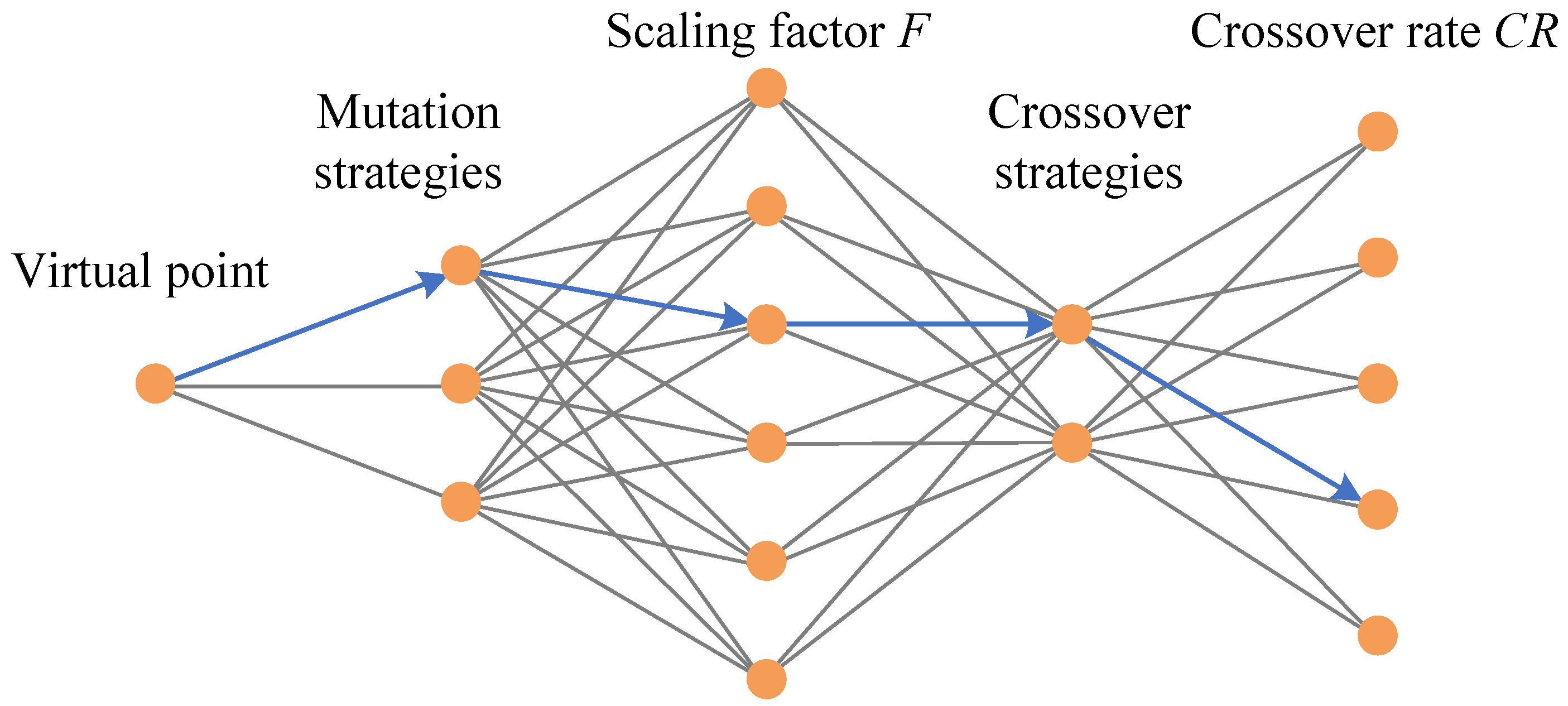Previously, many techniques have been developed to relieve this issue, such as ensemble and adaption techniques [28,30,31]. In this study, we implement the adaption technique to DE. Specifically, we form the genetic strategies and parameters of DE into a directed acyclic graph, in which each path indicates a combination of the genetic strategies and parameters. As the pheromone trails and property always enable the ant colony to find a reasonable path from the graph, an ant colony optimization (ACO) is adopted to search for effective combinations during the evolution. The hybridization of ACO and DE exhibits the effective search capability of DE that has been proved in previous studies [4,26,32]. Furthermore, it can dynamically optimize the algorithm configurations to improve the adaptive capability of DE, such that higher-quality solutions can be obtained for all three optimization models.

In summary, this paper has the following contributions.

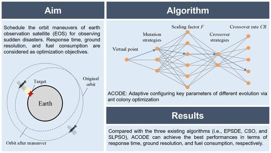
(i) We investigate the orbit maneuver optimization problem considering diverse user requirements. In the problem, a satellite is selected from a set of satellites and transferred to a new orbit based on appropriate maneuvers (i.e., the velocity increment and maneuver moment) to respond to an emergency observation request. By analyzing orbit coverage and dynamics, we build three optimization models that optimize response time, ground resolution, and fuel consumption, respectively, to satisfy different user requirements.

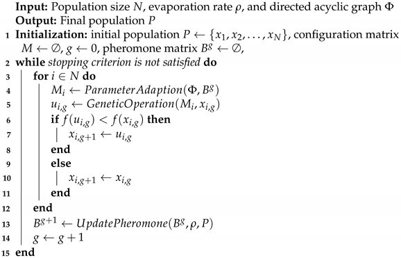
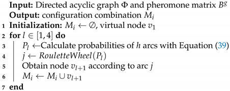
(ii) To solve the proposed optimization models, we implement an adaptive differential evolution based on graph search. In the algorithm, key algorithm components (i.e., crossover strategies, mutation strategies, and control parameters) are formed into a directed acyclic graph and an ACO is adopted to find reasonable combinations of configurations during the evolution. The implemented algorithm is a hybrid of ACO and DE, therefore it is named ACODE.

(iii) We conduct simulation experiments to verify the efficiency of ACODE. The ACODE is compared with three representative algorithms including EPSDE [33], CSO [34], and SLPSO [35] in simulation scenarios where multiple EOSs are requested to observe a ground target. The simulation results show the superiority of ACODE.

This paper is organized as follows. Section 2 details the orbit coverage and dynamics analysis, as well as three optimization models. Section 3 and Section 4 introduce the solution method and simulation experiments, respectively. Finally, the conclusions are remarked by Section 5.

2. Problem Description

In this section, we elaborate on the orbit maneuver optimization problem based on orbit coverage and dynamics calculations, followed by three optimization models with different optimization objectives (i.e., response time, fuel consumption, and ground resolution). As a part of the satellite system design, orbit maneuver optimization is associated with many complicated environmental factors. Therefore, some reasonable assumptions are adopted to simplify the problem.

(i) There are some perturbations (e.g., atmospheric drag, solar radiation pressure, and third body effects) that have negative impacts on the operation of the satellite. We only consider $J_2$ perturbation of Earth oblateness in the model, which is a common assumption in existing studies on orbit design problems [6,32,36].

(ii) Assume that the sensor equipped on each satellite is visible to the ground target when the satellite flies in the sunshine and the sunshine time is from 6:00 to 18:00 local time. Further, the other factors that may affect the imaging such as clouds and weather conditions, as well as the altitude of ground targets are assumed to be negligible.

(iii) Each satellite is assumed to be independent. Therefore, the orbit maneuver of a satellite does not affect the flying of another satellite.

(iv) The time required by the satellite to process task information and start the rocket engine is assumed to be negligible.

(v) The ground target is assumed to be a point target. Hence, the ground target can be imaged by the satellite once the satellite passes over it.

Main notations used in this section are displayed in Table 1.

Table 1. Notations.

Notations	Description
$\lambda$, ${\lambda }_h$, ${\lambda }_{max}$, and ${\lambda }_{min}$	Actual, horizon-, maximum, and minimum Earth’s angular radius
$\eta$, ${\eta }_c$, ${\eta }_h$, ${\eta }_{max}$, and ${\eta }_{min}$	Actual, center, horizon-, maximum, and minimum boresight angle of the sensor
$R_E$	Earth’s radius
$r_{sat}$	Distance between the Earth’s center and the satellite
$\gamma$	Intermediate angle
$\left[{lat}_s,{lon}_s\right]$	Latitude and longitude of a subsatellite point
a	Semimajor axis
e	Eccentricity
i	Inclination
$\mathsf{\Omega }$ and $\dot{\mathsf{\Omega }}$	Longitude of ascending node and its time variation
$\omega$ and $\dot{\omega }$	Argument of perigee and its time variation
$\theta$, M, and E	True, mean, and eccentric anomaly
P	Period for an orbit
$\mu$	Earth’s gravitational parameter
$t_0$	Time since perigee at the initial epoch
h	Angular momentum of the satellite
${\mathbf{r}}^O$ and ${\mathbf{r}}^I$	Position vectors of the satellite in PQW and ECI frames
${\mathbf{v}}^O$	Velocity vector of the satellite in PQW frame
$D_{imag}$	Satellite altitude over the ground target
$H_{new}$	Orbital altitude of the satellite after maneuvering
$\mathsf{\Delta }v$ and $\mathsf{\Delta }{v}_{max}$	Velocity increment and the allowed maximum velocity increment for maneuvering
$t_m$	Maneuver moment
$t_t$	Time when the satellite receives the observation task
$T_r$	Response time
$\left[t_s,t_e\right]$	Sunshine time window of a ground target
T	Maximum response time required by users
R	Minimum ground resolution required by users

2.1. Orbit Coverage Analysis

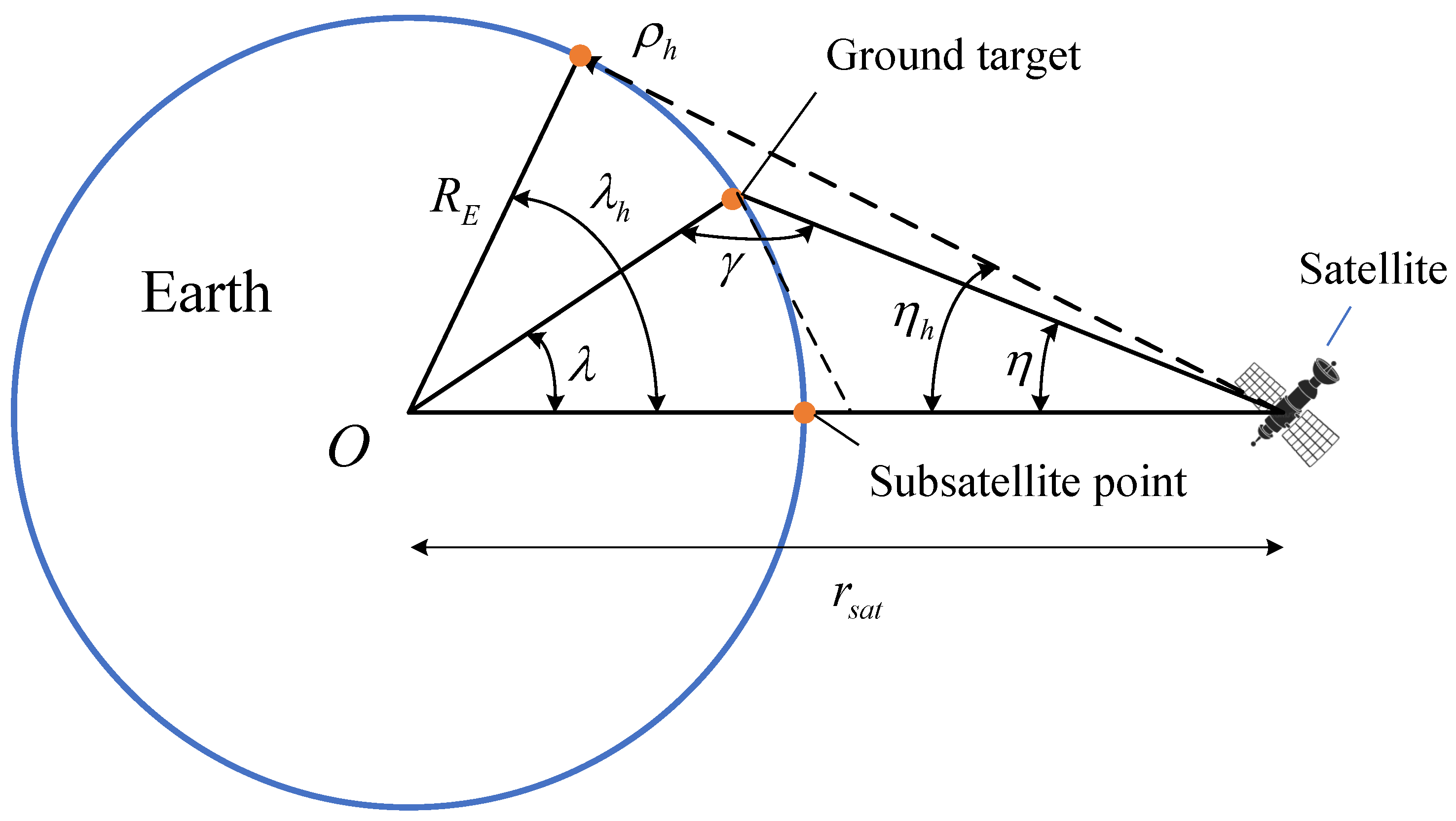
The visibility between a satellite and a ground target depends on many factors, such as the location of the ground target (i.e., longitude and latitude), the orbit elements, and the field of view (FOV) of the satellite. To conduct the orbit coverage analysis, we assume that the Earth is a round body, the orbit is approximately circular, and the FOV on the ground is rectangular as in [32,37]. The ground target is visible to the satellite when it lies in the FOV, which can be determined by calculating the longitudes and latitudes of four vertices. A typical satellite coverage on the Earth is shown in Figure 1.

Figure 1. Satellite coverage on the Earth.

As Figure 1 shows, the Earth’s angular radius ${\lambda }_h$ defines the half-ground range that may visible to the satellite, which can be expressed by

$$cos{\lambda }_h=\frac{R_E}{r_{sat}},$$

(1)

where $R_E$ is the Earth’s radius, and $r_{sat}$ is the distance between the Earth’s center and the satellite. The slant range to the horizon, ${\rho }_h$, can be written as

$${\rho }_h=\sqrt{{r_{sat}}^2-{R_E}^2}.$$

(2)

However, in practical applications, due to some limitations such as the imaging angle of the sensor and sunshine conditions, the actual half ground range would be smaller than ${\lambda }_h$. Hence, a general expression for the slant range to any point, $\rho$, can be expressed by [38]

$$\rho =R_{E}cos\gamma +r_{sat}cos\eta ,$$

(3)

$$sin\gamma =\frac{r_{sat}sin\eta }{R_E},$$

(4)

where $\gamma$ is the intermediate angle and $\eta$ is the boresight angle of the satellite (i.e., half of the sensor angle). Afterward, the half-ground range from the subsatellite point can be calculated by

$$sin\lambda =\frac{\rho sin\eta }{R_E}.$$

(5)

For the satellite equipped with a scanning sensor, the geometry of the FOV is no longer symmetrical about the subsatellite point, requiring more processing to obtain the ground range angle. Given the center boresight angle ${\eta }_c$ of the satellite, the maximum and minimum ground-range angles from the subsatellite point can be obtained. Specifically, the maximum and minimum boresight angles can be written as [38]

$${\eta }_{max}={\eta }_c+\eta ,$$

(6)

$${\eta }_{min}={\eta }_c-\eta .$$

(7)

Then, the maximum and minimum Earth’s angular radiuses (i.e., ${\lambda }_{max}$ and ${\lambda }_{min}$) can be obtained according to Equations (5)–(7). Since the sensor of the satellite can be rotated on multiple axes, in this study we assume that the sensor half-angle equals ${\eta }_{max}$ and the Earth’s angular radius equals ${\lambda }_{max}$ for convenience. Define the latitude and longitude of the subsatellite point as $\left[{lat}_s,{lon}_s\right]$, the latitudes and longitudes of the four vertices of the FOV can be calculated by $\left[{lat}_s+{\lambda }_{max},{lon}_s+{\lambda }_{max}\right]$, $\left[{lat}_s+{\lambda }_{max},{lon}_s-{\lambda }_{max}\right]$, $\left[{lat}_s-{\lambda }_{max},{lon}_s+{\lambda }_{max}\right]$, and $\left[{lat}_s-{\lambda }_{max},{lon}_s-{\lambda }_{max}\right]$, respectively.

According to the latitude and longitude information of the FOV, the latitude and longitude information of the ground target, the positions of the satellite at each moment, as well as the right ascension of Greenwich at the initial moment, we can obtain the key orbit performance indices of a satellite [39], such as the response time [32,40]. The response time is defined as the time required from when a request is received to observe a ground target until the satellite can observe it. The method that assesses whether the target lies in the FOV at moment t, as well as the response time $t_{imag}$ can be found in [32]. Moreover, the calculation method of the latitude and longitude of the subsatellite point at each moment is introduced in the next section.

2.2. Orbit Dynamics Model

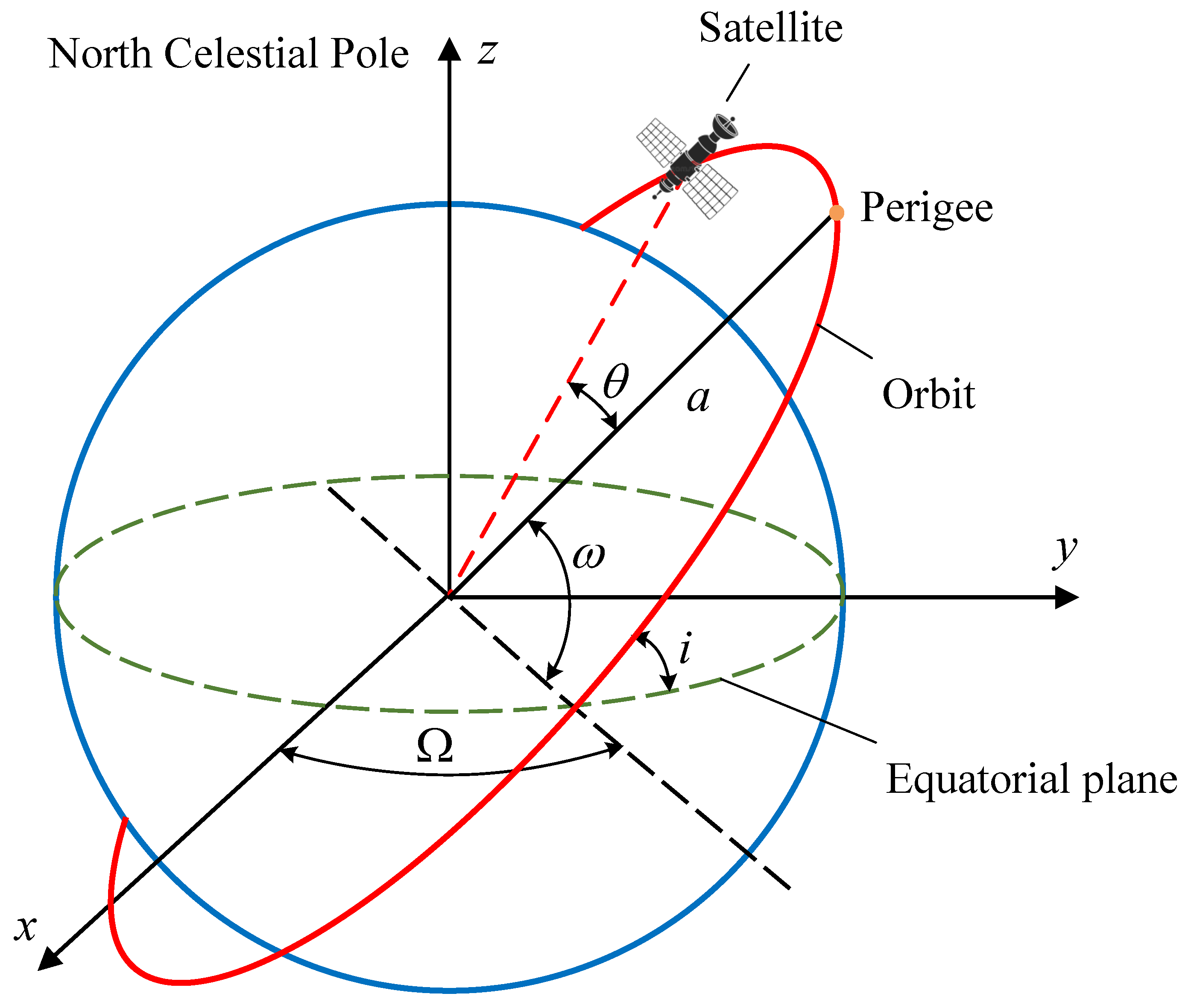
The position of a satellite in its orbit can be obtained by using six orbit elements, including semimajor axis a, eccentricity e, inclination i, longitude of ascending node $\mathsf{\Omega }$, argument of perigee $\omega$, and true anomaly $\theta$, as Figure 2 shows. By using the orbit elements, we can calculate the position of the satellite, as well as the latitude and longitude of each subsatellite point at each moment. In this section, we briefly introduce the calculation methods, and more detailed derivation steps can be found in [41].

Figure 2. Geocentric equatorial frame and the orbital elements.

Given a satellite flying around the Earth, it is well-known that the period P for an orbit of the satellite is calculated by

$$P=\frac{2\pi }{\sqrt{\mu }}{a}^{3/2},$$

(8)

where $\mu$ is the Earth’s gravitational parameter. Then, the time $t_0$ since perigee at the initial epoch can be calculated as

$$t_0=\frac{M}{2\pi }P,$$

(9)

where M is the initial mean anomaly. According to Kepler’s equation, M can be calculated by

$$M=E-esinE,$$

(10)

where E is the eccentric anomaly, which yields the relation with true anomaly $\theta$ as

$$tan\frac{E}{2}=\sqrt{\frac{1-e}{1+e}}tan\frac{\theta }{2}.$$

(11)

Given a time change $\mathsf{\Delta }t$, the longitude of ascending node $\mathsf{\Omega }$, argument of perigee $\omega$ at the moment $t=t_0+\mathsf{\Delta }t$ can be expressed by

$$\mathsf{\Omega }=\mathsf{\Omega }+\dot{\mathsf{\Omega }}\mathsf{\Delta }t,$$

(12)

$$\omega =\omega +\dot{\omega }\mathsf{\Delta }t,$$

(13)

where $\dot{\mathsf{\Omega }}$ and $\dot{\omega }$ are time variations of $\mathsf{\Omega }$ and $\omega$, which are determined by $J_2$ perturbation of Earth oblateness. The expressions of $\dot{\mathsf{\Omega }}$ and $\dot{\omega }$ are written as

$$\dot{\mathsf{\Omega }}=\left[\frac{3}{2}\frac{\sqrt{\mu }{J}_2{R}_E^2}{{\left(1-e^2\right)}^2{a}^{7/2}}\right]cosi,$$

(14)

$$\dot{\omega }=\dot{\mathsf{\Omega }}\frac{5/2{sin}^{2}i-2}{cosi},$$

(15)

where $J_2=1.083\times {10}^{-3}$. The orbit elements are updated by repeating Equations (9)–(13) at each moment t. Meanwhile, the newly found true anomaly $\theta$ at the moment t can be used to calculate the state vector of the satellite in the perifocal coordinate coordinate system (PQW). The satellite position vector ${\mathbf{r}}^O$ and velocity vector ${\mathbf{v}}^O$ in the PQW frame can be expressed by

$${\mathbf{r}}^O=\frac{h^2}{\mu }\frac{1}{1+ecos\theta }\left\{\begin{array}{c}cos\theta \\ sin\theta \\ 0\end{array}\right\},$$

(16)

$${\mathbf{v}}^O=\frac{\mu }{h}\left\{\begin{array}{c}-sin\theta \\ e+cos\theta \\ 0\end{array}\right\},$$

(17)

where h is the angular momentum of the satellite, yielding a relation with the semimajor axis a as below

$$a=\frac{h^2}{\mu }\frac{1}{1-e^2}.$$

(18)

Particularly, the position vectors ${\mathbf{r}}^O$ can be transformed to the Earth-centered inertial (ECI) frame through the transformation matrix $R^{I/O}$ ($C\equiv cos$ and $S\equiv sin$) written as

$$\begin{array}{cc}\hfill & R^{I/O}=\hfill \\ \hfill & \left[\begin{array}{ccc}{C}_{\omega }{C}_{\mathsf{\Omega }}-C_i{S}_{\omega }{S}_{\mathsf{\Omega }}& -S_{\omega }{C}_{\mathsf{\Omega }}-C_i{S}_{\mathsf{\Omega }}{C}_{\omega }& S_i{S}_{\mathsf{\Omega }}\\ C_{\omega }{S}_{\mathsf{\Omega }}+C_i{S}_{\omega }{C}_{\mathsf{\Omega }}& -S_{\omega }{S}_{\mathsf{\Omega }}+C_i{C}_{\mathsf{\Omega }}{C}_{\omega }& -S_i{C}_{\mathsf{\Omega }}\\ S_{\omega }{S}_i& C_{\omega }{S}_i& C_i\end{array}\right],\hfill \end{array}$$

(19)

by

$${\mathbf{r}}^I=R^{I/O}{\mathbf{r}}^O,$$

(20)

where ${\mathbf{r}}^I$ is the satellite position in the ECI frame. Meanwhile, ${\mathbf{r}}^I$ can be expressed in the Rotating Earth-fixed frame by [4]

$${\mathbf{r}}^{I^{\prime }}=\left[\begin{array}{ccc}cos\theta & sin\theta & 0\\ -sin\theta & cos\theta & 0\\ 0& 0& 1\end{array}\right]{\mathbf{r}}^I,$$

(21)

which can be written in vector notation

$${\mathbf{r}}^{I^{\prime }}=X\widehat{\mathbf{I}}+Y\widehat{\mathbf{J}}+Z\widehat{\mathbf{K}}.$$

(22)

Define a notation $r=\sqrt{X^2+Y^2+Z^2}$, the latitude and longitude of the subsatellite point can be calculated by

$${lat}_s={sin}^{-1}\left(Z/r\right),$$

(23)

$${lon}_s=\left\{\begin{array}{cc}{cos}^{-1}\left(\frac{X}{rcos{lat}_s}\right),\hfill & \frac{Y}{r}>0\hfill \\ {360}^{\circ }-{cos}^{-1}\left(\frac{X}{rcos{lat}_s}\right),\hfill & \mathrm{otherwise}\hfill \end{array}\right..$$

(24)

Based on the above equations, the position of the satellite, as well as the latitude and longitude of each subsatellite point at each moment can be obtained.

Furthermore, in this study, the orbit maneuver focuses on how to move a satellite in the same plane, which can be treated as a co-orbital rendezvous problem [42]. In the co-orbital rendezvous problem, two satellites are assumed to be located in the same orbit and one satellite maneuvers its orbit by two-impulse Hohmann transfer to catch up with the other one. Therefore, a velocity increment $\mathsf{\Delta }v$ at the moment $t_m$ is considered to calculate the orbit elements before and after maneuvering based on orbit equations.

2.3. Formulation of the Optimization Problem

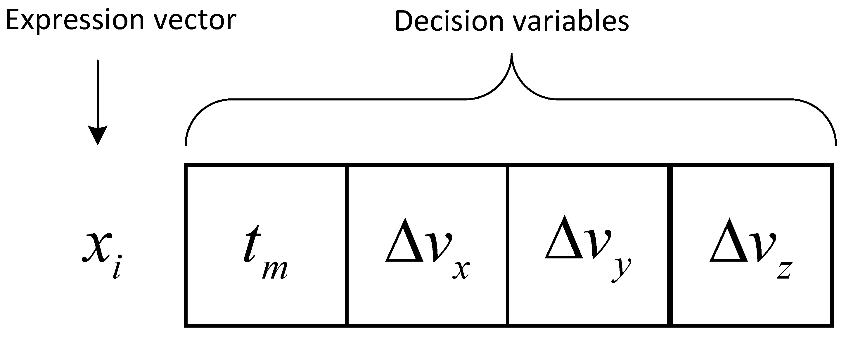
As mentioned above, the optimization problem aims to find appropriate velocity increment $\mathsf{\Delta }v$ and maneuver moment $t_m$ to obtain a reasonable scheduling scheme for transferring the satellite. Hence, $\mathsf{\Delta }v$ and $t_m$ can be considered as decision variables of the optimization problem, and they are constrained by

$$-\mathsf{\Delta }{v}_{max}\le \mathsf{\Delta }vs.\le \mathsf{\Delta }{v}_{max},$$

(25)

$$0<t_m<t_t+T.$$

(26)

Since $\mathsf{\Delta }v$ is associated with the capacity of fuel, which is the key parameter of the satellite remained lifetime, constraint (25) ensures that the velocity increment is limited to a reasonable range. Here $\mathsf{\Delta }{v}_{max}$ represents the maximum allowed velocity increment and the negative value indicates the velocity in the reverse direction. Constraint (26) defines the range of a feasible maneuver moment (when the satellite starts its rocket engine). Furthermore, there are other constraints introduced in the following.

$$D_{imag}/{10}^6\le R,$$

(27)

$$250\times {10}^3\le H_{new}\le 1300\times {10}^3,$$

(28)

$$t_s\le t_t+T_r\le t_e,$$

(29)

$$T_r\le T.$$

(30)

To obtain sufficient information from a single observation result, constraint (27) guarantees that the ground resolution is smaller than the required resolution, in which the ground resolution is associated with the satellite altitude over the ground target divided by the horizontal number of pixels. When the satellite is transferring its orbit, the change of orbit altitude should be limited to a reasonable range to ensure the stable operation of the satellite. As the satellite altitude is typically between 250 and 1300 km [43], constraint (28) is carried out to limit the satellite altitude after maneuvering. Constraint (29) is used to ensure that the observation moment lies in the sunshine time window. Furthermore, as timeliness is crucial for emergency observation tasks, we use constraint (30) to limit the maximum response time of the satellite.

In practical applications, users require different solutions depending upon the purpose. To satisfy diverse user requirements, we build three models considering response time, ground resolution, and fuel consumption as objectives, respectively, which are written as

$$\begin{array}{cc}\hfill & f_3=min{T}_r,\hfill \\ \hfill s.t.& Constraints\left(25\right)\text{–}\left(29\right).\hfill \end{array}$$

(31)

$$\begin{array}{cc}\hfill & f_2=min\left(D_{imag}/{10}^6\right),\hfill \\ \hfill s.t.& Constraints\left(25\right),\left(26\right),\left(28\right)\text{–}\left(30\right).\hfill \end{array}$$

(32)

$$\begin{array}{cc}\hfill & f_1=min\mathsf{\Delta }v,\hfill \\ \hfill s.t.& Constraints\left(26\right)\text{–}\left(30\right).\hfill \end{array}$$

(33)

The calculation processes of objectives are as follows. During the optimization process, appropriate decision variables (i.e., velocity vector increment $\mathsf{\Delta }v$ and maneuver moment $t_m$) will be searched by the algorithm under the constraints mentioned in Equations (31)–(33). Since the satellite conducts an impulsive maneuver whose direction and magnitude are determined by $\mathsf{\Delta }v$ at moment $t_m$ to transfer its orbit, the new state velocity vector at moment $t_m$ can be determined by decision variables. Then, the state velocity vector of the satellite can be transformed into the position vector represented by orbit elements by using Equations (19) and (20). As the satellite flies around the Earth, the position vector of the satellite changes with time. The changes in position vector can be tracked by Kepler’s equation coupled with orbit equations mentioned in Equations (8)–(18). Meanwhile, according to the position vector, the subsatellite point at the same moment can be obtained by Equations (21)–(24). The FOV of the satellite is determined by the subsatellite point at the same moment according to Equations (1)–(7) introduced in the orbit coverage analysis. When a FOV covers the target point, it indicates that the satellite can observe this target point. Thus, the first objective $f_1$ is calculated by the difference between the maneuver time $t_m$ and the time instance when the satellite can observe the target. In the second objective $f_2$, the satellite altitude is the distance between the satellite and the subsatellite point when the satellite can observe the target. As to the third objective $f_3$, it is determined by the decision variable $\mathsf{\Delta }v$ directly.

3. Adaptive Differential Evolution Algorithm Based on Graph Search

Differential evolution (DE) is an efficient population-based stochastic optimization approach for solving optimization problems over continuous space, and many variants of DE have been implemented in engineering fields [30,44,45]. In this study, we conduct problem-specific modifications on the framework of an adaptive DE, named ACODE, first proposed in [31] that concerned data clustering problems, to solve the orbit maneuver optimization problem. The ACODE can be treated as a hybridization of DE and ACO, which will be detailed in this section after a brief introduction to the classical DE.

3.1. Classical DE Algorithm

Typically, the DE includes four basic steps [46]: Initialization, mutation, crossover, and selection.

(i) Initialization. This step randomly creates an initial population consisting of N individuals. When the iteration number $G=0$, the i-th individual is initialized in the search space constrained by the minimum bound $X_{min}=\{x_{min}^1,x_{min}^2,\dots ,x_{min}^D\}$ and the maximum bound $X_{max}=\{x_{max}^1,x_{max}^2,\dots ,x_{max}^D\}$, according to the following method

$$\begin{array}{cc}\hfill & x_{i,0}^j=x_{min}^j+rand(0,1)\times (x_{max}^j-x_{min}^j),\hfill \\ \hfill & j\in \{1,2,\dots ,D\},\hfill \end{array}$$

(34)

where $rand(0,1)$ is a uniformly distributed number within $[0,1]$ and D is the number of dimensions.

(ii) Mutation. The mutation operation perturbs a target vector $X_{i,G}$ from the current generation to obtain a donor vector $V_{i,G}$, which can be written as

$$V_{i,G}=X_{r_1^i,G}+F·(X_{r_2^i,G}-X_{r_3^i,G}),$$

(35)

where F is the scaling factor, which is a positive control parameter for scaling the difference vectors. The indices $r_1^i$, $r_2^i$, and $r_3^i$ are mutually exclusive integers randomly chosen from the range $[1,N]$ and they are different from the base vector index i.

(iii) Crossover. The crossover operation can improve the diversity of the population by exchanging the components of the donor vector $V_{i,G}$ with the target vector $X_{i,G}$ to form the trial vector $U_{i,G}=\left\{u_{i,G}^1,u_{i,G}^2,\dots ,u_{i,G}^D\right\}$. There are two kinds of commonly used crossover strategies, including exponential (i.e., two-point modulo) and binomial (i.e., uniform). The exponential crossover makes the trial vector contains a sequence of consecutive components taken from the parent vector. The structure of the trial vector can be expressed by

$$u_{i,G}^j=\left\{\begin{array}{cc}{v}_{i,G}^j,\hfill & \mathrm{if}j\in \{k,{⟨k+1⟩}_n,\dots ,{⟨k+L-1⟩}_n\},\hfill \\ x_{i,G}^j,\hfill & \mathrm{for}\mathrm{all}\mathrm{other}j\in [1,D].\hfill \end{array}\right.$$

(36)

where ${⟨j⟩}_n$ is a modulo function with modules D, k and L are two integers randomly chosen from $[1,D]$. On the other hand, the binomial strategy can be outlined as

$$u_{i,G}^j=\left\{\begin{array}{cc}{v}_{i,G}^j,\hfill & \mathrm{if}({rand}_j[0,1]\le CR\mathrm{or}j=j_{rand}),\hfill \\ x_{i,G}^j,\hfill & \mathrm{otherwise}.\hfill \end{array}\right.$$

(37)

where $CR$ is the crossover rate and $j_{rand}$ is a randomly chosen index lying in the interval $[1,D]$.

(iv) Selection. The selection operation determines whether the target or the trial vector survives to the next generation according to the objective function, which is described as

$$X_{i,G+1}=\left\{\begin{array}{cc}{U}_{i,G},\hfill & \mathrm{if}f\left(U_{i,G}\right)\le f\left(X_{i,G}\right),\hfill \\ X_{i,G},\hfill & \mathrm{otherwise}.\hfill \end{array}\right.$$

(38)

Once an initial population is created, the mutation, crossover, and selection strategies are repeated until a stopping criterion is satisfied to obtain promising solutions. It should be noted that different mutation strategies demarcate a DE scheme from other schemes. Except for the mutation strategy introduced above, there are some other well-known mutation strategies, such as “DE/best/1”, “DE/best/2”, “DE/rand/2”, “DE/rand-to-best/1”, “DE/current-to-pbest/1”, “DE/current-to-rand/1”, etc. [46].

3.2. ACODE Algorithm

The performance of DE highly depends on four key components, i.e., mutation strategy, crossover strategy, scaling factor F, and crossover rate $CR$ [31]. We transform these components into a directed acyclic graph and implement an ant colony optimization-based adaptive DE algorithm to conduct the optimization process.

3.2.1. Directed Acyclic Graph Formed by Configurations

An example of the directed acyclic graph formed by configurations is shown in Figure 3. The graph includes five levels, of which a virtual point lies in the first level to gather all ants and the remaining four levels represent four key components (i.e., mutation strategy, crossover strategy, scaling factor F, and crossover rate $CR$), respectively. Every node in each level indicates a candidate configuration, and the nodes of two adjacent levels are fully connected. A path that starts from the first level and terminates at the fifth level can be treated as a combination of four candidate configurations, as the blue path in Figure 3 shows. Mathematically, the directed acrylic graph can be described by $\mathsf{\Phi }=\{V,E\}$, where V is the set of nodes and $E\subseteq V\times V$ indicates directed arcs. The pheromone trail on the arcs connecting $v\in V$ to adjacent nodes in the next level is recorded by pheromone vector $B_v$. Hence, the length of $B_v$ depends on the number of nodes in the next level. According to empirical considerations [31,33,46], the candidate configurations we used in this paper are summarized in Table 2.

Figure 3. An example of the directed acyclic graph formed by key components of DE.

Table 2. Candidate configurations.

Components	Candidate Values or Strategies
Mutation strategy	“DE/rand/1”, “DE/current-to-pbest/1”, and “DE/current-to-rand/1”
Crossover strategy	binomial and exponential
Scaling factor F	0.4, 0.5, 0.6, 0.8, 0.9, and 1.1
Crossover rate $CR$	0.1, 0.4, 0.6, 0.9, and 0.99

3.2.2. Framework of ACODE

The framework of ACODE is displayed in Algorithm 1. The algorithm starts with the initialization of a population P with size N, configuration matrix M, iteration counter g, and pheromone matrix $B^g$ (line 1). Particularly, the number of individuals in P equals the number of ants. Then, the algorithm runs until the stopping criterion is satisfied (lines 2–11). Every ant at each iteration is utilized to find a reasonable combination of configurations from the graph, and the combination is recorded in M (line 4). $M_i$ indicates the configuration combination of the i-th individual and it is implemented to evolve individual $x_{i,g}$ (line 5). The offspring $u_{i,g}$ is compared with $x_{i,g}$ to determine which solution is preserved into the next generation (lines 6–9). Finally, the pheromone matrix $B^{g+1}$ that would be used in the next generation is updated according to the fitness information in line 10.

3.2.3. Solution Representation and Initialization

As above-mentioned, we consider the velocity increment $\mathsf{\Delta }v$ and maneuver moment $t_m$ as decision variables. During the optimization process, the decision variables are used to calculate the positions of the satellite expressed by orbit elements, while the objectives are determined by position vectors, as introduced in Section 2. The velocity increment $\mathsf{\Delta }v$ is the magnitude of the change in the velocity vector, which can be represented by three velocities (i.e., $\mathsf{\Delta }{v}_x$, $\mathsf{\Delta }{v}_y$, and $\mathsf{\Delta }{v}_z$) on three axes of the Cartesian coordinate system. Here the X axis is directed to the eccentricity vector, Z axis is in the direction of the satellite’s angular momentum which lies perpendicular to the orbital plane, and the Y axis completes the right-hand set of co-ordinate axis. Therefore, a chromosome should be composed of velocity increments in three dimensions and the moment when the maneuver occurs. Figure 4 shows the representation of a chromosome, where $x_i$ is the expression vector while $t_m$, $\mathsf{\Delta }{v}_x$, $\mathsf{\Delta }{v}_y$, and $\mathsf{\Delta }{v}_z$ are decision variables. Since the satellite conducts a coplanar maneuver, the velocity increment $\mathsf{\Delta }{v}_z$ always equals 0. Nevertheless, we still include $\mathsf{\Delta }{v}_z$ in the chromosome for computation convenience. In addition, we generate the initial population randomly and the boundaries of decision variables are determined by constraints (25) and (26). Since the search space of each variable is large and the performance of DE algorithm is seriously influenced by the diversity of the initial population, the initial population should be uniformly distributed in the search space. We use the Latin hypercube sampling (LHS) to generate the initial population. The LHS is a statistical method that can generate a quasi-random sampling distribution, which has been widely applied in other studies to obtain a high-quality initial population [47].

Algorithm 1: Framework of ACODE.

Figure 4. An illustration of the chromosome representation.

3.2.4. Parameters Adaption Based on ACO

Based on the directed acyclic graph, we conduct the parameter adaption by utilizing an ACO method. Specifically, each ant searches for a reasonable combination (i.e., path) for configuring an individual according to the pheromone trail on each arc in the graph. Given a node v from which an ant departs, there would be h candidate arcs that can be chosen. The probability $p_j$ for picking arc j is written as

$$p_j=\frac{B_{v,j}^g}{{\sum }_{j=1}^h{B}_{v,j}^g},$$

(39)

where $B_{v,j}^g$ is the pheromone trail on arc j with the starting node v at the g-th iteration. The process of parameter adaption is shown in Algorithm 2. In the algorithm, an ant departs from the virtual node $v_1$ and travels through four nodes in the remaining four levels. At the l-th level, all probabilities for choosing arcs connecting starting node $v_l$ with all nodes in the next level are calculated based on Equation (39) and recorded in $P_l$ (line 3). Then, roulette wheel selection (i.e., $RouletteWheel\left(\right)$) is adopted to choose an arc j that determines the node $v_{l+1}$ (i.e., end node of arc j) at the $(l+1)$-th level (lines 4–5). The roulette wheel selection is a well-known stochastic selection method, in which the probability for the selection of an arc is proportional to the pheromone trails on it. The above steps are repeated until a path consisting of four arcs is obtained. This algorithm is embedded into Algorithm 1 by executing once for each individual.

Algorithm 2:$ParameterAdoption\left(\right)$.

3.2.5. Pheromone Update

In Algorithm 1, the pheromone trails of the whole graph at the generation g is recorded by a pheromone matrix $B^g$. The pheromone trail on each arc is updated at the end of each iteration by the following method

$$\mathsf{\Delta }{\tau }_{v,j}^g=\frac{{\sum }_{x_t\in P_j^g}|f\left(x_{t,g+1}\right)-f\left(x_{t,g}\right)|}{{\sum }_{i=1}^N|f\left(x_{t,g+1}\right)-f\left(x_{t,g}\right)|},$$

(40)

$$B_{v,j}^{g+1}=(1-\rho )·B_{v,j}^g+\mathsf{\Delta }{\tau }_{v,j}^g,$$

(41)

where $\mathsf{\Delta }{\tau }_{v,j}^g$ is the pheromone increment on arc j with starting node v at the g-th iteration, $P_j^g$ is the set of individuals who use the configurations corresponding to arc j at the g-the iteration, and $\rho$ is the evaporation rate. Equation (40) indicates that the pheromone increment on an arc is determined by accumulated fitness improvements of individuals who passed this arc divided by that of all individuals. The pheromone trail $B_{v,j}^{g+1}$ on arc j with starting node v at the $(g+1)$-th iteration is updated by pheromone increment $\mathsf{\Delta }{\tau }_{v,j}^g$ and pheromone trail $B_{v,j}^g$ at the g-the iteration, as well as evaporation rate $\rho$ in Equation (41). Further, to avoid premature convergence, the Max–Min ant system [48] is implemented in this study to limit the pheromone level on each arc within a range [0.1, 0.9].

4. Computational Experiments

To demonstrate the efficiency of ACODE on the proposed problem, simulation experiments are conducted in this section. All algorithms are coded in Matlab and run on a 64-bit Windows OS with Intel Core(TM) i5-8265U, 1.6 GHz, and 8 GB RAM.

4.1. Scenario Settings

We assume a set of scenarios in which three satellites are requested to observe four ground targets within 12 h (from 1 December 2020 14:00:00 to 2 December 2020 02:00:00, Beijing time). At the initial moment (i.e., 1 December 2020 14:00:00), each ground target is invisible to each satellite. Once an observation task is received, an appropriate satellite would be selected from these satellites to undertake orbital maneuvers to accomplish the task according to users’ requirements. The initial orbital elements are displayed in Table 3, where the first column is the satellite ID and the other columns indicate semimajor axis a, inclination i, right ascension of the ascending node $\mathsf{\Omega }$, eccentricity e, argument of perigee $\omega$, and mean anomaly M. The four ground targets are randomly located in low-latitude, mid-latitude, high-latitude, and higher-latitude areas, and their geographical information is summarized in Table 4. The maximum scanning angle of the satellite, maximum response time, minimum ground resolution, and maximum velocity increment predefined by users are set to ${45}^{\circ }$, 12 h, 2 m, and 300 m/s, respectively. Moreover, the maximum number of fitness evaluations (FEs) of the algorithm is set to 50,000 and the evaporation rate $\rho$ is set to 0.8 according to pre-experiments.

Table 3. Initial orbital elements of satellites.

ID	a (m)	e	i (rad)	$\mathbf{\Omega }$ (rad)	$\mathit{\omega }$ (rad)	M (rad)
1	6,878,140	3.59426 × ${10}^{-16}$	97.0346	250.884	0	0
2	6,878,140	4.55556 × ${10}^{-18}$	97.0346	10.8840	0	2.61014 × ${10}^{-16}$
3	6,878,140	1.79873 × ${10}^{-16}$	97.0346	130.884	0	5.08063 × ${10}^{-15}$

Table 4. Geographical information of ground targets.

Target ID	Latitude	Longitude
1	0°	62°W
2	41°N	70°E
3	50°S	146°W
4	45°N	116°E

4.2. Simulation Results

The ACODE is implemented to solve the three optimization models with different optimization objectives based on the generated scenarios. The experiment results are summarized in Table 5, in which the columns indicate scenarios, satellites selected to accomplish observation tasks, maneuver moment $t_m$, velocity increments ($\mathsf{\Delta }{v}_x$ and $\mathsf{\Delta }{v}_y$), and objective values ($f_1$, $f_2$, and $f_3$) of the three optimization models. Particularly, the scenario index is composed of the ground target ID and optimization objective. For instance, T1O1 means in this scenario the satellites are requested to observe ground target 1 and the optimization objective is $f_1$ involved by the first optimization model. Here $f_1$, $f_2$, and $f_3$ are response time, ground resolution, and fuel consumption, respectively. Note that the minimum fuel consumption is represented by minimum velocity increment, as discussed in Section 2. Although only one objective is considered in each scenario, we provide the values of the other two objectives corresponding to the optimal solution of the scenario. The value of the optimized objective considered in each scenario is in boldface.

Table 5. Simulation results.

Scenario	Selected Satellite ID	${\mathit{t}}_{\mathit{m}}$	$\mathbf{\Delta }{\mathit{v}}_{\mathit{x}}$ (m/s)	$\mathbf{\Delta }{\mathit{v}}_{\mathit{y}}$ (m/s)	${\mathit{f}}_1$ (s)	${\mathit{f}}_2$ (m)	${\mathit{f}}_3$ (m/s)
T1O1	3	2020-12-1 14:49	−81.744079	288.2563	56821	1.34	299.62
T1O2	1	2020-12-1 14:10	286.203453	89.93099	36507	0.43	300.00
T1O3	1	2020-12-1 14:45	−65.113285	−9.637086	36507	1.08	65.82
T2O1	1	2020-12-1 14:59	123.578258	272.2139	6301	1.35	298.95
T2O2	3	2020-12-1 14:46	−155.259419	−256.6993	20440	0.44	300.00
T2O3	3	2020-12-1 14:00	3.676842	0.506845	19243	0.74	3.71
T3O1	2	2020-12-1 14:44	−224.161983	198.8964	4833	1.41	299.68
T3O2	2	2020-12-1 15:10	−252.270809	162.3559	40115	0.44	300.00
T3O3	1	2020-12-1 14:11	15.541757	−15.38881	9401	0.85	21.87
T4O1	3	2020-12-1 15:14	293.379811	−56.7	7705	1.01	298.81
T4O2	1	2020-12-1 14:45	−137.707437	−266.5268	38606	0.43	300.00
T4O3	1	2020-12-1 15:20	24.506321	31.81572	7859	0.95	40.16

¹ The values in boldface are optimized objectives in each scenario.

The results in Table 5 indicate that all scenarios can be well-addressed by ACODE. Furthermore, it can be observed that huge differences in objective values can be obtained if we execute the same observation task based on different optimization models. For example, T1O1, T1O2, and T1O3 are three scenarios in which the satellites are requested to observe ground target 1 with three different optimization objectives, respectively. The solution of T1O1 selects satellite 3 to execute the task and earns the minimum response time while yielding the poorest ground resolution compared with solutions of T1O2 and T1O3. More specifically, the solution of T1O1 decreases the response time by up to 84.44% and increases the ground resolution by up to 200.12% compared with the solutions of T1O2 and T1O3. Meanwhile, its fuel consumption is a little less than the solution of T1O2 that optimizes the ground resolution and much more than the solution of T1O3 that aims to find the minimum fuel consumption.

4.3. Algorithm Comparisons

To further demonstrate the superiority of ACODE, we compare it with three well-known evolutionary algorithms in existing studies, i.e., EPSDE [33], CSO [34], and SLPSO [35]. Particularly, EPSDE is an ensemble-based DE algorithm, in which a pool of mutation strategies along with a pool of corresponding control parameters compete to produce offspring individuals. CSO is a competitive swarm optimizer inspired by particle swarm optimization. In CSO, a pairwise competition mechanism is used to update the position of the particle that loses the competition by learning from the winner. Similarly, SLPSO adopts social learning mechanisms for particle swarm optimization. Meanwhile, a dimension-dependent parameter control method is embedded into the SLPSO to ease the burden of parameter settings.

The comparison results are summarized in Table 6, in which the last four columns are best, worst, mean, and standard deviation values of three optimization objectives over 10 runs obtained by all algorithms. Note that the fuel consumption is represented by the value of velocity increment. For each scenario, the best results are in boldface. Wilcoxon rank-sum tests with a significance level of 0.05 are used for the significance tests. It can be found that ACODE significantly outperforms EPSDE, CSO, and SLPSO in almost all scenarios, in terms of response time, ground resolution, and fuel consumption. Especially, the superiority of ACODE is more significant when it optimizes orbital maneuvers for observing ground target 1 in terms of response time (scenario T1O1) and ground target 2 in terms of fuel consumption (scenario T2O3).

Table 6. Algorithm comparison results.

Scenario	Algorithm	Best	Worst	Mean	Std.
T1O1	ACODE	56821	5682	5682	0
	EPSDE	5689	5721	5701.8	9.71
	CSO	5689	19,935	7124.8	4270.07
	SLPSO	5693	19,909	7194.9	4239.05
T1O2	ACODE	0.43	0.43	0.43	0
	EPSDE	0.43	0.47	0.45	0.01
	CSO	0.48	0.64	0.56	0.06
	SLPSO	0.49	0.63	0.55	0.04
T1O3	ACODE	65.82	65.82	65.82	0
	EPSDE	68.18	76.5	71.68	3.15
	CSO	67.34	80.74	74.85	3.6
	SLPSO	76.98	120.14	97.47	12.66
T2O1	ACODE	6301	6301	6301	0
	EPSDE	6308	6341	6324.5	10.76
	CSO	6311	6339	6322.5	9.11
	SLPSO	6355	19,146	10,222	5834.61
T2O2	ACODE	0.44	0.44	0.44	0
	EPSDE	0.45	0.47	0.46	0.01
	CSO	0.47	0.55	0.51	0.03
	SLPSO	0.44	0.58	0.5	0.04
T2O3	ACODE	3.71	3.81	3.72	0.03
	EPSDE	6.31	10.06	8.28	1.3
	CSO	4.78	11.89	6.95	2.24
	SLPSO	9.4	72.13	29.45	18.07
T3O1	ACODE	4833	4833	4833	0
	EPSDE	4848	4882	4858.4	9.77
	CSO	4888	5129	4944.3	66.58
	SLPSO	4843	9332	6236.6	2006.62
T3O2	ACODE	0.44	0.44	0.44	0
	EPSDE	0.45	0.51	0.47	0.02
	CSO	0.49	0.54	0.51	0.01
	SLPSO	0.46	0.58	0.5	0.04
T3O3	ACODE	21.87	21.87	21.87	0
	EPSDE	22.83	32.5	29.11	3.43
	CSO	23.93	29.52	27.11	1.68
	SLPSO	34.74	64.22	45.18	8.49
T4O1	ACODE	7705	7705	7705	0
	EPSDE	7723	7746	7732.7	7.4
	CSO	7726	7754	7738	8.06
	SLPSO	7769	7846	7804.1	24.92
T4O2	ACODE	0.43	0.44	0.43	0
	EPSDE	0.45	0.48	0.46	0.01
	CSO	0.47	0.6	0.51	0.04
	SLPSO	0.48	0.55	0.52	0.02
T4O3	ACODE	40.16	40.16	40.16	0
	EPSDE	42.91	46.58	45.07	1.16
	CSO	41.05	48.92	43.91	2.58
	SLPSO	45.07	74.64	60.88	9.85

¹ The values in boldface are the best results in each scenario.

It should be noted that EPSDE is similar to ACODE, as EPSDE ensembles a set of mutation strategies and corresponding control parameters in DE. Hence, EPSDE shows similar performance compared with ACODE for observing ground target 1 in terms of ground resolution (scenario T1O2). Nevertheless, ACODE is superior to EPSDE in other scenarios. The reasons can be twofold. First, EPSDE only ensembles mutation strategies and corresponding control parameters, while crossover strategies and corresponding control parameters that also can affect algorithm performance are not involved. On the contrary, ACODE considers both mutation strategies, crossover strategies, and their control parameters. Second, each component of EPSDE conducts the adaption independently while ACODE configures all components in a holistic manner, which is also the difference between ACODE and ensemble-based algorithms.

4.4. Experiments with Insufficient Satellite Resources

In the above sections, we calculate the solution of every satellite and select the most appropriate satellite out of three satellites to observe the ground target. The simulation results are obtained by the algorithm with sufficient satellite resources. However, since some satellites may be occupied by other tasks that cannot be interrupted when emergencies occur (i.e., some satellites may be infeasible for executing the observation task), it is interesting to investigate the impact of insufficient satellite resources on the orbital maneuver scheme and algorithm performance. Hence, this section analyzes the experiment results with different numbers of satellites based on the scenarios generated by removing satellites from the scenarios introduced in Section 4.1. Specifically, the one-satellite scenarios in this section preserve satellite 1, the two-satellite scenarios preserve satellite 1 and satellite 2, and the three-satellite scenarios are the same as before.

The simulation results are presented in Figure 5. Each figure indicates the simulation results for observing the same ground target, and the same color means the simulation results in the scenarios that consider the same optimization model. Moreover, to understand the trade-off among three objectives, we normalize all results into [0, 1], and a smaller value indicates a better solution in a direction. Since we generate the scenarios by removing satellites from the scenarios that already have solutions in Section 4.2, some scenarios would have the same solution as before. For example, the solution schemes of three scenarios that observe target 1 while optimizing the ground resolution with different numbers of satellites select satellite 1 to execute the task. Hence, the results of scenarios T1O2-one-satellite, T1O2-two-satellite, and T1O2-three-satellite are the same, as Figure 5a shows. On the other hand, other solutions indicate that the number of satellites significantly affects the algorithm results. For example, scenarios T1O1-one-satellite, T1O1-two-satellite, and T1O1-three-satellite select three different satellites to execute the task, respectively. To observe ground target 1 with the aim of optimizing response time, satellite 2 is selected in the two-satellite scenario and the response time is increased by 249.93% compared with the solution of the three-satellite scenario, as Figure 5a shows.

Figure 5. Simulation results by varying the number of satellite. (a) Ground target 1, (b) ground target 2, (c) ground target 3, (d) ground target 4.

Furthermore, it can be found that with the increase in the number of satellites, the value of the optimization objective that corresponds to each optimization model can be significantly improved. However, the trade-off results among the three objectives show that the improvement on one objective may not always promote the improvement of other objectives. For example, the ground resolution for observing ground target 2 is significantly improved as the number of satellites increases from 1 to 3, while the fuel consumption is still very high and the response time is even increased, as Figure 5b shows.

5. Conclusions

In this paper, we investigate the orbital maneuver optimization problem of Earth observation satellites oriented to emergency tasks. Based on the analysis of orbit coverage and dynamics, we propose three kinds of optimization models that aim to, respectively, optimize response time, ground resolution, and fuel consumption, to satisfy diverse user requirements. Meanwhile, we implement an adaptive differential evolution algorithm based on graph search to solve the proposed optimization problems, which is named ACODE. The main feature of ACODE is to form the key components of DE into a directed acyclic graph and adopt an ACO method to search for combinations of these components from the graph, thereby adaptively configuring reasonable components for DE. The key components considered in this paper include mutation strategies, crossover strategies, as well as their corresponding control parameters, both of which can affect the performance of DE.

Finally, computational experiments are conducted to verify the proposed three optimization models and ACODE. The simulation results show that all simulation scenarios that consider different optimization objectives can be well-addressed by ACODE. Comparison experiments are also carried out to demonstrate the superiority of ACODE on the proposed problem. The comparison results indicate that ACODE is superior to three well-known algorithms (i.e., EPSDE, CSO, and SLPSO). Further, we find that insufficient satellite resources would affect the efficiency of the orbital maneuver scheme and algorithm.

In future studies, we would like to investigate the multi-objective optimization algorithm that can optimize the three optimization objectives simultaneously for better decision making operations.

References

- Wang, X.; Wu, G.; Xing, L.; Pedrycz, W. Agile earth observation satellite scheduling over 20 years: Formulations, methods, and future directions. IEEE Syst. J. 2020, 15, 3881–3892. [Google Scholar] [CrossRef]
- Verhegghen, A.; Kuzelova, K.; Syrris, V.; Eva, H.; Achard, F. Mapping Canopy Cover in African Dry Forests from the Combined Use of Sentinel-1 and Sentinel-2 Data: Application to Tanzania for the Year 2018. Remote Sens. 2022, 14, 1552. [Google Scholar] [CrossRef]
- Chen, J.; Tang, H.; Ge, J.; Pan, Y. Rapid Assessment of Building Damage Using Multi-Source Data: A Case Study of April 2015 Nepal Earthquake. Remote Sens. 2022, 14, 1358. [Google Scholar] [CrossRef]
- Chen, Y.; Mahalec, V.; Chen, Y.; He, R.; Liu, X. Optimal Satellite Orbit Design for Prioritized Multiple Targets with Threshold Observation Time Using Self-Adaptive Differential Evolution. J. Aerosp. Eng. 2015, 28, 04014066. [Google Scholar] [CrossRef]
- Savitri, T.; Kim, Y.; Jo, S.; Bang, H. Satellite Constellation Orbit Design Optimization with Combined Genetic Algorithm and Semianalytical Approach. Int. J. Aerosp. Eng. 2017, 2017, 1235692. [Google Scholar] [CrossRef] [Green Version]
- Sengupta, P.; Vadali, S.R.; Alfriend, K.T. Satellite Orbit Design and Maintenance for Terrestrial Coverage. J. Spacecr. Rocket. 2010, 47, 177–187. [Google Scholar] [CrossRef]
- Graham, K.F.; Rao, A.V. Minimum-Time Trajectory Optimization of Low-Thrust Earth-Orbit Transfers with Eclipsing. J. Spacecr. Rocket. 2016, 53, 289–303. [Google Scholar] [CrossRef] [Green Version]
- Wang, Z.; Grant, M.J. Optimization of Minimum-Time Low-Thrust Transfers Using Convex Programming. J. Spacecr. Rocket. 2017, 55, 586–598. [Google Scholar] [CrossRef]
- Zhang, C.; Topputo, F.; Bernelli-Zazzera, F.; Zhao, Y.S. Low-Thrust Minimum-Fuel Optimization in the Circular Restricted Three-Body Problem. J. Guid. Control Dyn. 2015, 38, 1501–1510. [Google Scholar] [CrossRef] [Green Version]
- Sadegh Mohammadi, M.; Naghash, A. Robust optimization of impulsive orbit transfers under actuation uncertainties. Aerosp. Sci. Technol. 2019, 85, 246–258. [Google Scholar] [CrossRef]
- Cheng, L.; Wang, Z.; Jiang, F.; Zhou, C. Real-Time Optimal Control for Spacecraft Orbit Transfer via Multiscale Deep Neural Networks. IEEE Trans. Aerosp. Electron. Syst. 2019, 55, 2436–2450. [Google Scholar] [CrossRef]
- Morante, D.; Sanjurjo-Rivo, M.; Soler, M.; Sánchez-Pérez, J.M. Hybrid multi-objective orbit-raising optimization with operational constraints. Acta Astronaut. 2020, 175, 447–461. [Google Scholar] [CrossRef]
- Song, Z.; Chen, X.; Luo, X.; Wang, M.; Dai, G. Multi-objective optimization of agile satellite orbit design. Adv. Space Res. 2018, 62, 3053–3064. [Google Scholar] [CrossRef]
- Appel, L.; Guelman, M.; Mishne, D. Optimization of satellite constellation reconfiguration maneuvers. Acta Astronaut. 2014, 99, 166–174. [Google Scholar] [CrossRef]
- Paek, S.W.; Kim, S.; de Weck, O. Optimization of Reconfigurable Satellite Constellations Using Simulated Annealing and Genetic Algorithm. Sensors 2019, 19, 765. [Google Scholar] [CrossRef] [Green Version]
- Sarno, S.; Guo, J.; D’Errico, M.; Gill, E. A guidance approach to satellite formation reconfiguration based on convex optimization and genetic algorithms. Adv. Space Res. 2020, 65, 2003–2017. [Google Scholar] [CrossRef]
- McGrath, C.N.; Macdonald, M. General Perturbation Method for Satellite Constellation Reconfiguration Using Low-Thrust Maneuvers. J. Guid. Control Dyn. 2019, 42, 1676–1692. [Google Scholar] [CrossRef] [Green Version]
- Soleymani, M.; Fakoor, M.; Bakhtiari, M. Optimal mission planning of the reconfiguration process of satellite constellations through orbital maneuvers: A novel technical framework. Adv. Space Res. 2019, 63, 3369–3384. [Google Scholar] [CrossRef]
- He, X.; Li, H.; Yang, L.; Zhao, J. Reconfigurable Satellite Constellation Design for Disaster Monitoring Using Physical Programming. Int. J. Aerosp. Eng. 2020, 2020, 8813685. [Google Scholar] [CrossRef]
- Wang, X.; Zhang, H.; Bai, S.; Yue, Y. Design of agile satellite constellation based on hybrid-resampling particle swarm optimization method. Acta Astronaut. 2021, 178, 595–605. [Google Scholar] [CrossRef]
- Hu, J.; Huang, H.; Yang, L.; Zhu, Y. A multi-objective optimization framework of constellation design for emergency observation. Adv. Space Res. 2021, 67, 531–545. [Google Scholar] [CrossRef]
- Pontani, M.; Conway, B.A. Particle swarm optimization applied to impulsive orbital transfers. Acta Astronaut. 2012, 74, 141–155. [Google Scholar] [CrossRef]
- Zhang, S.; Duan, H. Gaussian pigeon-inspired optimization approach to orbital spacecraft formation reconfiguration. Chin. J. Aeronaut. 2015, 28, 200–205. [Google Scholar] [CrossRef] [Green Version]
- dos Santos, D.P.S.; da Silva Formiga, J.K. Application of a genetic algorithm in orbital maneuvers. Comput. Appl. Math. 2015, 34, 437–450. [Google Scholar] [CrossRef]
- Shirazi, A. Analysis of a hybrid genetic simulated annealing strategy applied in multi-objective optimization of orbital maneuvers. IEEE Aerosp. Electron. Syst. Mag. 2017, 32, 6–22. [Google Scholar] [CrossRef] [Green Version]
- Yao, W.; Luo, J.; Macdonald, M.; Wang, M.; Ma, W. Improved Differential Evolution Algorithm and Its Applications to Orbit Design. J. Guid. Control Dyn. 2018, 41, 936–943. [Google Scholar] [CrossRef] [Green Version]
- Hitomi, N.; Selva, D. Constellation optimization using an evolutionary algorithm with a variable-length chromosome. In Proceedings of the 2018 IEEE Aerospace Conference, Big Sky, MT, USA, 3–10 March 2018; pp. 1–12. [Google Scholar] [CrossRef]
- Wu, G.; Mallipeddi, R.; Suganthan, P.N. Ensemble strategies for population-based optimization algorithms—A survey. Swarm Evol. Comput. 2019, 44, 695–711. [Google Scholar] [CrossRef]
- Mallipeddi, R.; Wu, G.; Lee, M.; Suganthan, P.N. Gaussian adaptation based parameter adaptation for differential evolution. In Proceedings of the 2014 IEEE Congress on Evolutionary Computation (CEC), Beijing, China, 6–11 July 2014; pp. 1760–1767. [Google Scholar] [CrossRef]
- Wu, G.; Mallipeddi, R.; Suganthan, P.N.; Wang, R.; Chen, H. Differential evolution with multi-population based ensemble of mutation strategies. Inf. Sci. 2016, 329, 329–345. [Google Scholar] [CrossRef]
- Wu, G.; Peng, W.; Hu, X.; Wang, R.; Chen, H. Configuring differential evolution adaptively via path search in a directed acyclic graph for data clustering. Swarm Evol. Comput. 2020, 55, 100690. [Google Scholar] [CrossRef]
- Chen, Y.; Mahalec, V.; Chen, Y.; Liu, X.; He, R.; Sun, K. Reconfiguration of satellite orbit for cooperative observation using variable-size multi-objective differential evolution. Eur. J. Oper. Res. 2015, 242, 10–20. [Google Scholar] [CrossRef]
- Mallipeddi, R.; Suganthan, P.; Pan, Q.; Tasgetiren, M. Differential evolution algorithm with ensemble of parameters and mutation strategies. Appl. Soft Comput. 2011, 11, 1679–1696. [Google Scholar] [CrossRef]
- Cheng, R.; Jin, Y. A Competitive Swarm Optimizer for Large Scale Optimization. IEEE Trans. Cybern. 2015, 45, 191–204. [Google Scholar] [CrossRef] [PubMed]
- Cheng, R.; Jin, Y. A social learning particle swarm optimization algorithm for scalable optimization. Inf. Sci. 2015, 291, 43–60. [Google Scholar] [CrossRef]
- Vandenrijt, J.F. Simulation and graphical representation of the orbit and the imaging parameter of Earth observation satellites. Acta Astronaut. 2005, 57, 186–196. [Google Scholar] [CrossRef]
- Zhu, K.J.; Li, J.F.; Baoyin, H.X. Satellite scheduling considering maximum observation coverage time and minimum orbital transfer fuel cost. Acta Astronaut. 2010, 66, 220–229. [Google Scholar] [CrossRef]
- Vallado, D.A. Fundamentals of Astrodynamics and Applications; Springer: Berlin/Heidelberg, Germany, 2001; Volume 12. [Google Scholar]
- Dong, Y.; Wei, X.; Tian, L.; Liu, F.; Xu, G. A Novel Double Cluster and Principal Component Analysis-Based Optimization Method for the Orbit Design of Earth Observation Satellites. Int. J. Aerosp. Eng. 2017, 2017, 6396032. [Google Scholar] [CrossRef]
- Buzzi, P.G.; Selva, D.; Hitomi, N.; Blackwell, W.J. Assessment of constellation designs for earth observation: Application to the TROPICS mission. Acta Astronaut. 2019, 161, 166–182. [Google Scholar] [CrossRef] [Green Version]
- Curtis, H. Orbital Mechanics for Engineering Students; Butterworth-Heinemann: Oxford, UK, 2013. [Google Scholar]
- Edlund, E.M. Interception and rendezvous: An intuition-building approach to orbital dynamics. Am. J. Phys. 2021, 89, 559–566. [Google Scholar] [CrossRef]
- Somma, G.L.; Lewis, H.G.; Colombo, C. Sensitivity analysis of launch activities in Low Earth Orbit. Acta Astronaut. 2019, 158, 129–139. [Google Scholar] [CrossRef] [Green Version]
- Biswas, P.P.; Suganthan, P.N.; Wu, G.; Amaratunga, G.A.J. Parameter estimation of solar cells using datasheet information with the application of an adaptive differential evolution algorithm. Renew. Energy 2019, 132, 425–438. [Google Scholar] [CrossRef]
- Wu, G.; Shen, X.; Li, H.; Chen, H.; Lin, A.; Suganthan, P.N. Ensemble of differential evolution variants. Inf. Sci. 2018, 423, 172–186. [Google Scholar] [CrossRef]
- Das, S.; Suganthan, P.N. Differential Evolution: A Survey of the State-of-the-Art. IEEE Trans. Evol. Comput. 2011, 15, 4–31. [Google Scholar] [CrossRef]
- Zhao, Z.; Yang, J.; Hu, Z.; Che, H. A differential evolution algorithm with self-adaptive strategy and control parameters based on symmetric Latin hypercube design for unconstrained optimization problems. Eur. J. Oper. Res. 2016, 250, 30–45. [Google Scholar] [CrossRef]
- Stützle, T.; Hoos, H.H. MAX–MIN Ant System. Future Gener. Comput. Syst. 2000, 16, 889–914. [Google Scholar] [CrossRef]
Publisher’s Note: MDPI stays neutral with regard to jurisdictional claims in published maps and institutional affiliations. |
© 2022 by the authors. Licensee MDPI, Basel, Switzerland. This article is an open access article distributed under the terms and conditions of the Creative Commons Attribution (CC BY) license (https://creativecommons.org/licenses/by/4.0/).