Uncertainty-Guided Depth Fusion from Multi-View Satellite Images to Improve the Accuracy in Large-Scale DSM Generation

Abstract

The generation of digital surface models (DSMs) from multi-view high-resolution (VHR) satellite imagery has recently received a great attention due to the increasing availability of such space-based datasets. Existing production-level pipelines primarily adopt a multi-view stereo (MVS) paradigm, which exploit the statistical depth fusion of multiple DSMs generated from individual stereo pairs. To make this process scalable, these depth fusion methods often adopt simple approaches such as the median filter or its variants, which are efficient in computation but lack the flexibility to adapt to heterogenous information of individual pixels. These simple fusion approaches generally discard ancillary information produced by MVS algorithms (such as measurement confidence/uncertainty) that is otherwise extremely useful to enable adaptive fusion. To make use of such information, this paper proposes an efficient and scalable approach that incorporates the matching uncertainty to adaptively guide the fusion process. This seemingly straightforward idea has a higher-level advantage: first, the uncertainty information is obtained from global/semiglobal matching methods, which inherently populate global information of the scene, making the fusion process nonlocal. Secondly, these globally determined uncertainties are operated locally to achieve efficiency for processing large-sized images, making the method extremely practical to implement. The proposed method can exploit results from stereo pairs with small intersection angles to recover details for areas where dense buildings and narrow streets exist, but also to benefit from highly accurate 3D points generated in flat regions under large intersection angles. The proposed method was applied to DSMs generated from Worldview, GeoEye, and Pleiades stereo pairs covering a large area (400 km²). Experiments showed that we achieved an RMSE (root-mean-squared error) improvement of approximately 0.1–0.2 m over a typical Median Filter approach for fusion (equivalent to 5–10% of relative accuracy improvement).

1. Introduction

The number of very high-resolution (VHR) optical satellite sensors has increased drastically over the last two decades. These sensors, such as WorldView I-IV, Pleiades A/B, PleiadesNeo, SkySat, GaoFen, KompSat, etc. [1], are capable of collecting images at a resolution of one meter or less with large swaths, adding petabytes of data to the archives every day. As a result, the available VHR images have reached a point where every single site on the Earth can be covered by multiple such images from different perspectives [1,2]. Therefore, using VHR satellite imagery to reconstruct high-quality digital surface models (DSM) has attracted increasing attention, as with more images, it is possible to exploit redundant observations by fusing these multi-view images, including in-track, cross-track, and cross-sensor datasets [3,4].

Existing solutions can be categorized into two paradigms:

(1)

A full multi-image matching (MIM) solution simultaneously exploits the collinearity relations of multiple images to triangulate 3D points in the object space [5,6];

(2)

A multi-view stereo (MVS) approach first constructs multiple stereo pairs and then performs bi-stereo matching to generate individual DSMs, followed by a DSM fusion (or depth fusion) over these DSMs [2,7].

MIM solutions often require a process called bundle adjustment [8] to be applied to all the images prior to triangulating the 3D points; this process simultaneously adjusts the position of each satellite image. To perform a bundle adjustment (BA), tie points across multiple images are needed to build observational equations. The extraction of reliable and multi-image tie points can be particularly challenging for satellite images; indeed, most of these images are from different dates with severe differences in illumination, posing many difficulties in the extraction of consistent tie points among multiple images. Furthermore, BA alone may not be sufficient to achieve good geometric accuracy for the position estimation when the convergence angles (or base-to-height ratio) among the satellite images are relatively small and this can lead to large vertical errors, especially due to the fact that a BA relies only on sparse tie points.

In contrast, a MVS solution directly performs the fusion on the DSM generated by individual stereo pairs, which are previously relatively orientated (instead of a full bundle adjustment for all the images). This has three advantages over the MIM solutions: first, the relative orientation only requires tie points between a selected pair of images instead of all images, which is much less demanding. Second, since the single DSM registration and fusion are performed utilizing every single 3D point, the vertical errors can be better accommodated than in a BA process that uses only sparse tie points. Third, the MVS solution is more flexible and easier to implement; since single DSMs are generated independently, one can implement different methods and different sensor models for DSM generation of data from different sources. Therefore, the MVS approach is generally more favored when processing multi-view satellite images. For example, as noted in [5], MIM approaches implemented in practical systems, due to their high computation needs, often seek efficiency-driven solvers that tend to avoid global optimizations, and thus may suffer more from noise and incompleteness in textureless regions. Similarly, Bhushan et al. [9] performed an experiment on Skysat imagery (frame-camera-based), and hypothesized that a MVS solution generally outperformed alternatives as it could better exploit redundant measurements generated by single stereo pairs.

In the “IARPA Multi-view stereo 3D mapping challenge” workshop [10], it was concluded that selecting the right stereo pairs can be decisive to the finally fused DSM. Therefore, existing solutions focus on the selection of stereo pairs for fusion [4,11], whereas the fusion algorithms have been less investigated. Among the fusion algorithms used in existing MVS frameworks, most adopt a simple median filter or its variants along the depth direction. A basic median filter assumes that the measurements at each pixel location of the DSM grid follow a Gaussian distribution, and thus that the median value of multiple DSMs can be a good estimate of the expected measurement. A few fusion approaches have proposed minor modifications to extend the assumption of a single Gaussian kernel to multiple ones [2], or to adopt postprocessing techniques that utilize the associated orthophotos [12] to enforce image segmentation constraints. However, these fusion methods often assume that the contributions of each measurement are identical, and rarely consider the use of a priori knowledge inherited from the photogrammetric stereo processing that is already existing in the MVS pipeline.

The dense image matching (DIM) algorithms, as a necessary step of the pipeline, compute dense correspondences between two images to support the 3D point triangulation. During this process, the DIM algorithm measures the potential of pixel-level matches, for which it produces an algorithm-specific matching confidence (or uncertainty) score. We hypothesize that this matching uncertainty can be readily used to guide the depth fusion process and advance the results of the state-of-the-art approaches.

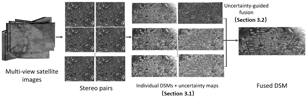
The Proposed Work

In this paper, we propose a new fusion algorithm that incorporates uncertainty measures of DIM into the merging process. In a typical MVS pipeline, a per-pixel matching uncertainty is computed and associated with every pixel of the generated DSM. The proposed DSM fusion algorithm adapts these pixel-level uncertainties so that the contribution of each pixel can be adaptively determined in order to advance the final fusion results. The main contributions of the work are threefold:

• A scalable procedure that uses the uncertainty information of the dense matching to better fuse depth maps;
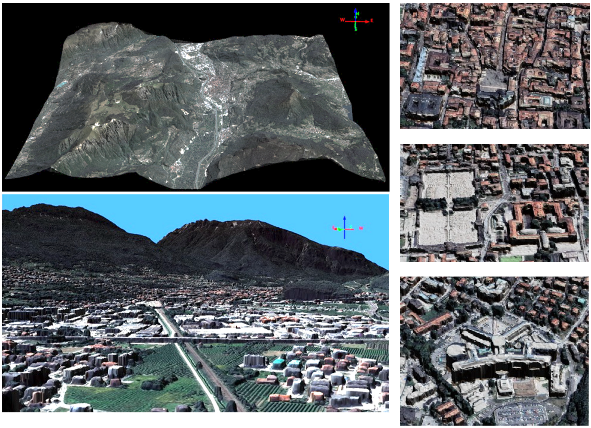
• An evaluation of the proposed procedure performances using three different satellite datasets (WorldView-2, GeoEye, and Pleiades) acquired over a complex urban landscape;
• An RMSE improvement of 0.1–0.2 m (5–10% of relative accuracy improvement considering the achieved 2–4 m of the final RMSE on different evaluation cases) against LiDAR reference data over a typical median filter.

2. State of the Art

Most existing solutions for depth fusion fall under the contexts of robotics and 3D scene modeling using depth sensors, where per-view depth maps are fused following probabilistic models [13] with focuses on frame-level depth registration and noise removal [14]. Recent developments include learning-based methods such as the application of 2D/3D CNN (Convolutional Neural Networks) to regress from multiple depth maps to a final depth map, exploiting latent space for Gaussian-process based fusion as well as for depth refinement through synthetic datasets [15]. However, these approaches mostly assume continuous or near-continuous video collections from sensors such as RGB-D (depth) sensors or full-motion video sensors. Under these scenarios, it is easy to assume the same probabilistic distributions, as the depth maps are often of the same or similar quality. In contrast, the individual depth maps (or DSMs) from the satellite images are drastically different due to factors such as temporal changes, resolution differences, and geometric configurations of individual stereo pairs. These differences further complicate the fusion problem, preventing approaches from making strong assumptions about the consistencies of individual measurements. For example, a single mean and variance for a pixel in the DSM may not be the best assumption, since there may exist multiple correct values due to temporal changes of the location (e.g., building demolition, vegetation variations, etc.). Relevant attempts have considered the fusion of multiresolution 3D data in the object space; however, they mostly focused on the use of more efficient data structures to fuse accurate 3D measurements such as those from high-resolution image-based or LiDAR point clouds [16,17].

A line of research in MVS satellite reconstruction focuses on selecting “good” stereo pairs to produce high-quality individual DSMs and prepare for a better fusion [2,3,4]. It has been concluded that the intersection angles and sun angle differences are important factors of concern [4,11]. Generally, the intersection angle is positively correlated to the achievable accuracy of point measurement, while larger angles introduce larger parallax, which will lead to occlusions, gaps for urban objects, and, ultimately, reduction of overall DSM accuracy. On the other hand, a smaller intersection angle creates smaller parallaxes in stereo matching and will generally lead to a better completeness, while due to the low base-to-height ratio, potentially producing 3D points with higher uncertainties. The importance of the sun angle difference was only recently noted by existing works [4,11]. Two images collected under different sun incidence angles were noted to have larger radiometric inconsistency, which could lead to errors in stereo matching. Thus, the sun angle differences negatively impact the resulting accuracy of the DSM.

Few works have aimed at the development of efficient methods for depth fusion of satellite-based DSMs. Facciolo et al. [2] hypothesized a bimodal state of a point in space to represent leaf on/off; the authors first applied a clustering algorithm on the height values to differentiate terrain and nonterrain points, and then retained only the centroid value of the lowest cluster. Qin [7] incorporated orthophotos to provide object boundary information through kernel-based filtering to derive image-edge-aware DSMs, leading to improvements of object boundaries in the resulting DSM. A similar approach adopted semantic information derived from the orthophotos and adaptively used class-specific parameters for kernel-based filtering [12]. Rumpler et al. [18] proposed a probabilistic filtering scheme for range image integration that avoided volumetric voxel representation and selected a final depth from continuous values in object space. Unger et al. [19] projected a number of pairwise disparity maps onto a reference view pair and fused maps by estimating a probability density function using the reprojection uncertainties and their photo-consistencies; they then selected the most probable one from the probability distribution.

The remainder of this paper is organized as follows: Section 3 describes our proposed depth fusion method in detail, Section 4 presents some experiments and describes the accuracy analysis, Section 5 discusses the results and observations found from experiments, and Section 6 concludes this paper by discussing the pros and cons of the proposed methods.

3. Methodology

A general workflow of the proposed approach is shown in Figure 1. The process starts with several satellite images taken from different perspectives (multi-view images) and then constructs a few stereo pairs, followed by a pairwise reconstruction to generate individual DSMs. During the individual DSM generation, our approach also derives uncertainty maps (details in Section 3.1) and generates the fused DSM using both the individual DSMs and uncertainty maps through our proposed uncertainty-guided fusion method (details in Section 3.2).

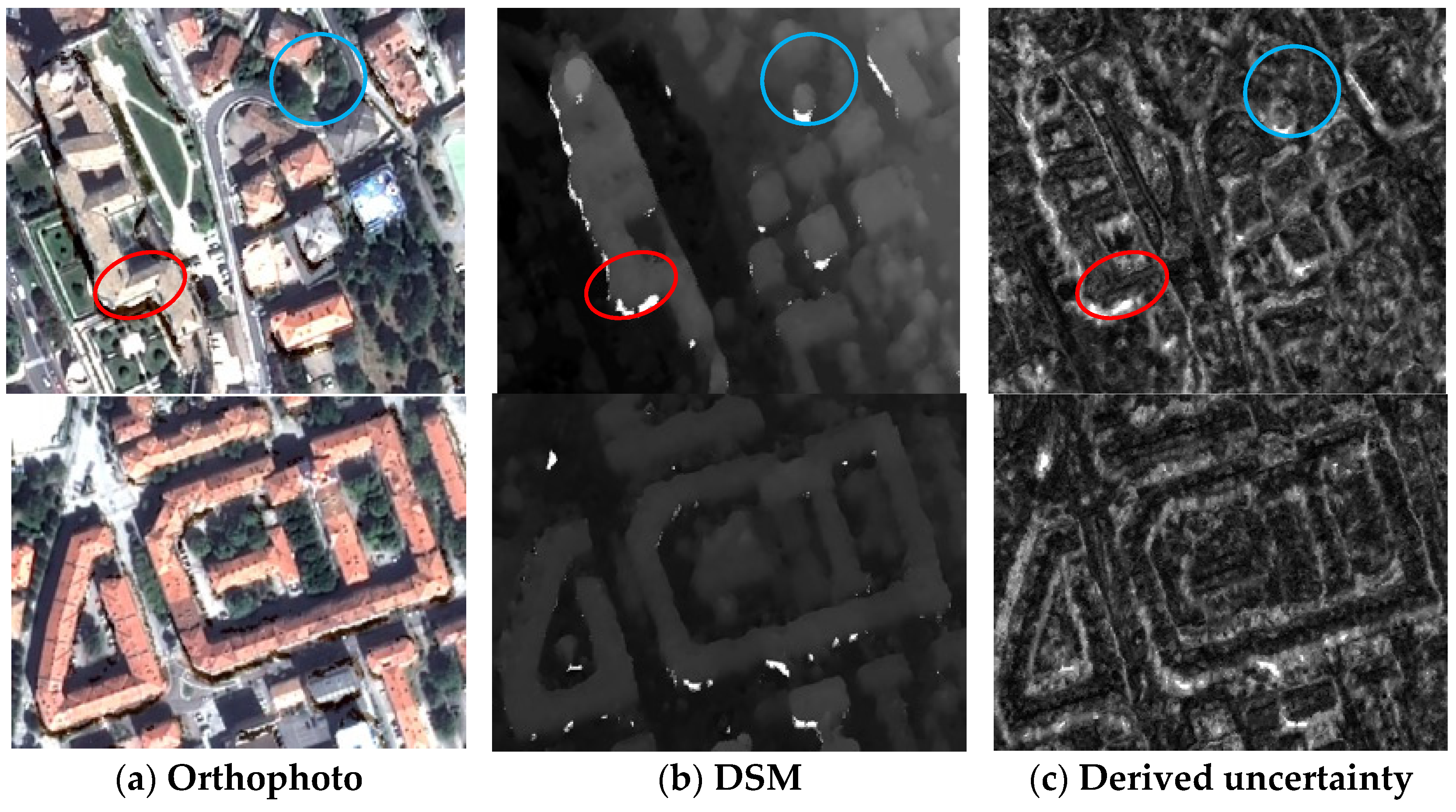
3.1. The Uncertainty Metric through Dense Image Matching

Dense image matching (DIM) algorithms for depth/disparity generation can deliver per-pixel a posteriori confidence metrics. For example, a simple normalized cross-correlation (NCC) matching in photogrammetry [20] offers the NCC coefficient, which indicates how similar two candidate correspondences with their surrounding textures are and represents a level of confidence/uncertainty for the matches. Our framework derives the uncertainty from an SGM algorithm [21,22]; thus, we can obtain for each pixel $p$ in its disparity (i.e., in the epipolar image) its corresponding uncertainty $u_p$. Since SGM performs the matching following a cost function that evaluates both the similarity of pixels and the spatial smoothness of the disparity values, we use its a posteriori cost metric $U$ to represent the matching uncertainty, described as follows:

$$U\left(D\right)={{\displaystyle \sum }}_{p}S\left(p,D_p\right)+{{\displaystyle \sum }}_{q\in N_p}{P}_{1}T\left[|D_p-D_q|=1\right]+{{\displaystyle \sum }}_{q\in N_p}{P}_{2}T\left[|D_p-D_q|>1\right],$$

(1)

where $U\left(D\right)$ refers to the a posteriori cost metric, minimized with respect to the disparity values $D$. The first term ${{\displaystyle \sum }}_{p}S\left(p,D_p\right)$ denotes the sum of similarity cost given the disparity $D$, and the similarity is calculated using the Census cost [23]. The second and third terms impose smoothness constraints onto the disparity map, and $N_p$ denotes the neighboring pixels (4- or 8-connected neighborhood) of a pixel $p$. $T[·]$ is a logical function that returns 1 if the argument is true, and 0 otherwise. $P_1$ and $P_2$ respectively penalize small and large disparity jumps to enforce the smoothness of the geometric surface. In practice, these two parameters are often set as constant, where $P_2$ generally is larger than $P_1$ to penalize large disparity changes (i.e., noise). Here, the Census cost is computed using a fixed $7\times 9$ window to maximize the use of memory of a “double” floating-point type for Census cost [24]; thus, the range of values of this metric is fixed as [0–63].

The solution of $D$ minimizing Equation (1) is obtained through multipath dynamic programming [21], where for each pixel $p$ with a given disparity value $D_p$, the algorithm computes an aggregated cost considering the smoothness constraints to determine the best disparity value for each pixel. The smallest aggregated cost for each pixel p, denoted as $U_p$, is taken as the uncertainty of the matching. The value of $U_p$ depends on the Census cost and the parameters of $P_1$ and $P_2$, which are fixed in their value and ranges; thus, $U_p$ also stays within a fixed range of values. Therefore, $U_p$ is image agnostic and can be compared among DSMs generated from different stereo pairs.

Two examples of the derived uncertainty are shown in Figure 2; it can be observed that, in general, a high level of uncertainty is present in pixels located at large depth discontinuities, e.g., due to occlusions (see example in the red-circle region of Figure 2), as well as in vegetated areas (light blue region).

The uncertainty metric $U_p$ was initially associated with each pixel in the epipolar image and then projected onto the generated DSM during the stereo triangulation. We hypothesize that the uncertainty metric generally represents the quality of matching for each pixel. Therefore, a DSM point with a lower matching uncertainty would generally indicate a higher possibility for a correct match and the point should be “weighted” more heavily when computing the fused DSM values. It should be noted that the uncertainty values may favor pairs with smaller intersection angles, since these pairs generally yield smaller parallax, thus showing lower level of uncertainty for all pixels, especially under good radiometric conditions (i.e., stereo images with similar sun angles). On the other hand, “good matches” in pairs with small intersection angles may necessarily lead to higher vertical uncertainty. Therefore, a small uncertainty metric $U_p$ may indicate that a DSM point is the result of a good match (not an error), and its precision can be further determined by the geometry of the stereo pair (i.e., the intersection angle). Therefore, both factors (the uncertainty metric and intersection angle), if combined, reflect the accuracy of a DSM point. However, both of these two factors are probabilistic to the accuracy, and thus a simple weighted average based on any of two factors for fusion will be unlikely to generate statistically meaningful results, and these two factors must be considered in a single fusion scheme.

3.2. Uncertainty Guided DSM Fusion

Median as a robust measure: Median is known as a well-practiced statistical predictor that can robustly estimate expectations over a large number of observations under varying distributions. To understand how median values are used in fusion, we first consider the following probabilistic framework: we denote the height value of pixel location $p$ in a DSM $j$, generated from a single stereo pair as an independent and random variable $X_j~(\tilde{X},{\delta }_j)$, with its expectation $\mathrm{E}(X_j)=\tilde{X}$ as the actual height value. Given the limited precision in the image level matching, the theoretical geometric uncertainty in the vertical direction can be presented as the variance of this distribution ${\delta }_j$. Intuitively, the smaller the intersection angle is, the bigger the variance ${\delta }_j$ is, and more samples are needed to obtain a good estimation of the expectation. If we consider the mean of these random variables $\frac{{{\displaystyle \sum }}_j{X}_j}{N}$ ($j$ indexing over the $N$ DSMs), its expectation $\mathrm{E}\left(\frac{{{\displaystyle \sum }}_j{X}_j}{N}\right)$ remains $\tilde{X}$, and thus a measure such as the median can be applied to these observations to more robustly estimate the expectation. However, to achieve an estimate with high confidence, the number of observations is insufficient if we only consider observations for each pixel in the DSM grid. Therefore, to increase the number of samples, pixels within a window centered at the pixel $p$ are also considered.

Adaptive sample aggregation: Inspired by the edge-aware approach [7], we define the adaptive neighborhood by using the color information from the orthophoto, which assumes neighboring pixels with similar color share similar height values; thus, a weighted Gaussian function can be built based on the color/radiometry of the orthophoto as follows:

$$W\left(p\right)=e^{-\frac{{\left|\left|q-p\right|\right|}^2}{2{\delta }_s{}^2}-\frac{{\left|\left|C_q-C_p\right|\right|}^2}{2{\delta }_c{}^2}},$$

(2)

where $q$ refers to pixels in the vicinity of pixel $p$, defined here as a window centered at $p$; $C$ refers to the color of the pixels in the orthophoto; and ${\delta }_s$ and ${\delta }_c$ are their bandwidths and take the values of ${\delta }_s$ = 7 and ${\delta }_c$ = 20 (for 8-bit image). Similar pixels in the window for which $W\left(p\right)>0.5$ are then aggregated into a set ${\mathbb{N}}_c\left(p\right)$. Thus, for each pixel $p$ in a DSM $j$, we can augment observations to a set ${\mathbb{N}}_c\left(p\right)$. In this paper, we use the same ${\mathbb{N}}_c\left(p\right)$ for all DSM based on a single orthophoto (while it may vary if multiple orthophotos associated with the DSMs are available), and these height values for consideration are defined as follows:

$${\mathscr{H}}_c\left(p\right)=\left\{DS{M}_j\left(q\right)|,q\in {\mathbb{N}}_c\left(p\right),j=1,\dots ,M\right\},$$

(3)

where $M$ refers to the number of DSMs.

Matching confidence as a guide for median filtering: ${\mathbb{N}}_c\left(p\right)$ aggregates samples for each individual DSM guided by the orthophoto. Intuitively, taking the median value of the aggregated sample set of height ${\mathscr{H}}_c\left(p\right)$ over all DSMs may be a straightforward solution. However, the presence of a large number of errors within ${\mathscr{H}}_c\left(p\right)$ is the major hurdle; for example, DSMs generated from pairs with large intersection angles easily produce errors for structures with large relief differences due to occlusions, gaps, shadows, and missing points (Figure 3).

As mentioned before, we hypothesize that a DSM pixel with lower matching uncertainties indicates a lower likelihood that the height value of this pixel is an error. The idea is to utilize the matching uncertainty $U_p$ (Section 3.1) to separate these measurements into groups based on the likelihood of their being errors. Therefore, on top of the aggregated sample set ${\mathscr{H}}_c\left(p\right)$, we made the following modification: we first rank all samples according to their matching uncertainties $U_p$ (from low to high); based on the ranked sample, we divide them into $K$ groups ${\mathscr{H}}_{rc}^k\left(p\right)$ (with $K=2$ to allow sufficient observations in each group), and then we compute the median values $Me{d}_k$ for each of cumulated groups:

$$Me{d}_k=\{Median({{\displaystyle \cup }}_{j=1,..,k}{\mathscr{H}}_{rc}^j\left(p\right))\},$$

(4)

Intuitively, these $Me{d}_k$ values should contain increasing number of errors as K increases, despite the benefit of having more observations. $Me{d}_1$, as the most confident prediction, seems to be the natural choice. However, as we mentioned before, the uncertainty alone does not accurately reflect good measurements, as the intersection angle also plays a role. For example, if there is a good pair with very small intersection angle, samples of the first group (that with the lowest uncertainties) may mostly come from the DSM produced by that pair, and directly using $Me{d}_1$ as the fused value may not reach statistically meaningful estimation. Alternatively, since $Me{d}_1$ reflects the value with the lowest probability of being an error, we can therefore use it to verify whether the median value of the aggregated sample set ${\mathscr{H}}_c\left(p\right)$ is an error; here we denote:

$$Me{d}_{all}=Median\left({\mathscr{H}}_c\left(p\right)\right),$$

(5)

and devise our approach following a heuristic: if $Me{d}_{all}$ is similar to $Me{d}_1$, we take $Me{d}_{all}$ as the final fused value since the set ${\mathscr{H}}_c\left(p\right)$ contains more samples; if their difference is larger than a predefined threshold (as a decision criteria for error), $Me{d}_1$ is taken as the fused value.

We found that for complex urban objects with high and frequent relief changes, $Me{d}_{all}$ tended to overestimate the height of lower objects when these objects were occluded, which happened very often for stereo pairs with large intersection angles. Therefore, we re-adapted this formulation by only taking $Me{d}_1$ as the fused value if $Me{d}_{all}$ was bigger than $Me{d}_1$ over the error threshold. Hence this simple fusion algorithm can be written as shown in the following pseudo-code (Algorithm 1).

Algorithm 1: Pseudo code for the proposed fusion method

$\mathrm{Initiate} \mathrm{M} \mathrm{registered}: DS{M}_j$$; \mathrm{Orthophoto}: Im{g}_o$$; \mathrm{the} \mathrm{fused}: DS{M}_f$

$\mathrm{Blunder} \mathrm{Threshold}: \partial$

For $p$ in all pixels in $DS{M}_f$

For j in $DS{M}_j$

aggregate ${\mathbb{N}}_c\left(p\right)$ based on $Im{g}_o$ for $DS{M}_j$ (following Equation (2))

collect height samples ${\mathscr{H}}_c\left(p\right)$ (following Equation (3))

compute $Me{d}_1$ and $Me{d}_{all}$ (following Equations (4) and (5))

if $Me{d}_{all}$ − $Me{d}_1$ > $\partial$

$DS{M}_f\left(p\right)$ = $Me{d}_1$

else

$DS{M}_f\left(p\right)$ = $Me{d}_{all}$

The error threshold $\partial$ can be set as an empirical value or adaptively estimated based on the DSMs. In the experiments presented in the following section, $\partial =6 \mathrm{m}$ was used for the very-high-resolution image data (0.5 m resolution).

4. Experiments and Analyses

Some experiments were performed on a challenging test field located in Trento (Italy) [25,26]. The topography of this area features various types of land morphology, including high mountains with approximately 2000 m relief differences, flat regions with large and sparse manmade objects, dense urban regions with street corridors (high-rise buildings on both sides) as narrow as 5 m in width (less than 10 pixels), and a large river (Figure 4a) in the lower valley at 200 m a.s.l. Several stereo pairs of this area were collected from three different sensors, including WorldView-2, GeoEye, and Pleiades, covering an overlapped area of approximately $20\times 20 {\mathrm{km}}^2$. Rich reference data were available in this area, including a reference LiDAR DSM to serve as ground truth for accuracy validation, and GCPs (ground control points) for image georeferencing. To better assess (both qualitatively and quantitatively) the reconstruction results, three representative urban subregions (noted as the area of interest—AOI-1–3 hereafter) were selected, featuring various levels of building size and densities (Figure 4b). Details of these datasets and regions are further introduced in Section 4.1 and

Table 1. Details of the used satellite datasets over the Trento test field.

Datasets	Intersection Angle (degrees)	GSD (m)	Area (km2)	Year
Pleiades stereo pair 1	5.57	0.72	20 × 20	2012
Pleiades stereo pair 2	27.85	0.72	20 × 20	2012
Pleiades stereo pair 3	33.42	0.72	20 × 20	2012
GeoEye-1 stereo pair	30.30	0.50	10 × 10	2011
WorldView-2 stereo pair	33.71	0.51	17 × 17	2010

.

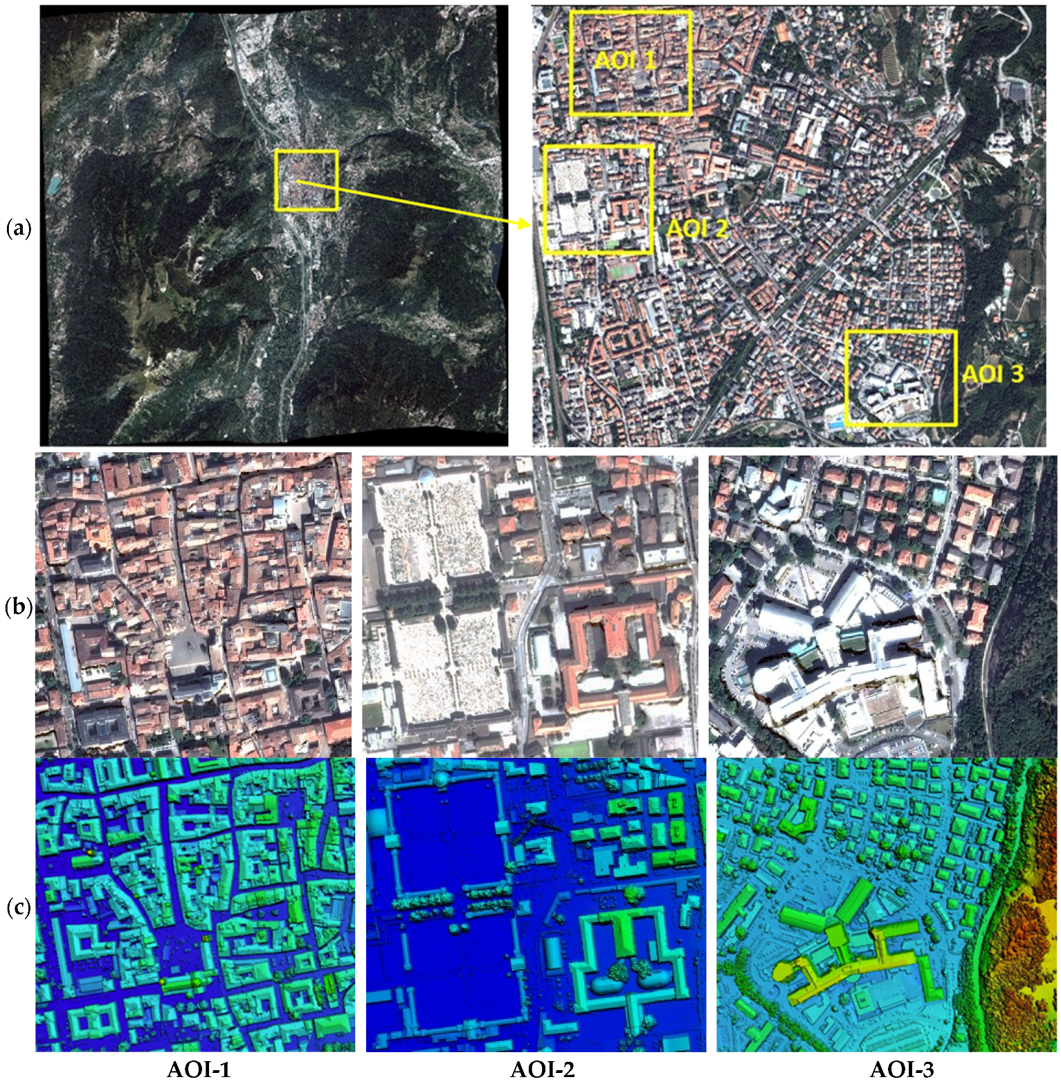
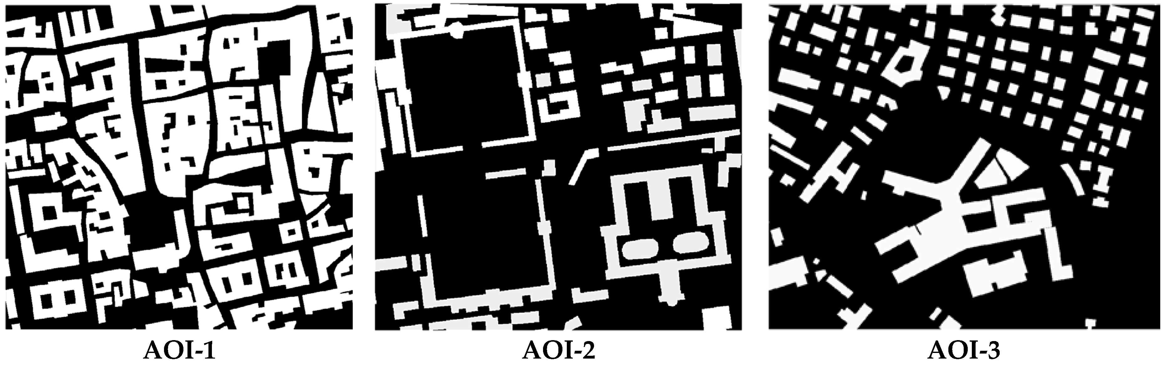
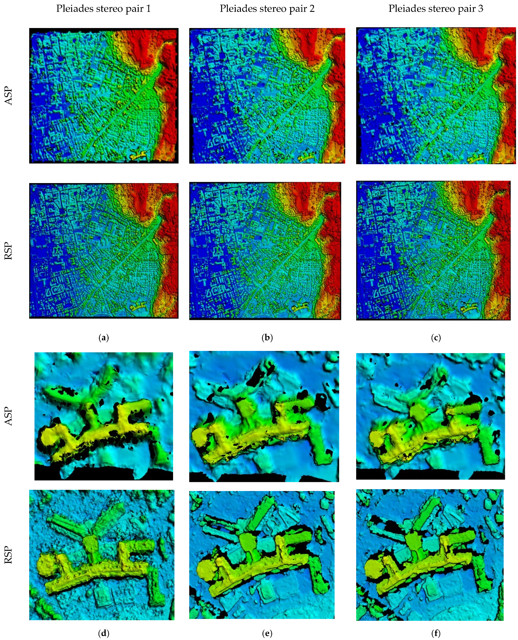
4.1. Experiment Dataset and Setup

A Pleiades tri-stereo product, a WorldView-2 stereo pair, and a GeoEye-1 stereo pair were considered (Table 1). The Pleiades tri-stereo images were divided into three stereo pairs in order to study the 3D reconstruction accuracy on stereo pairs with different acquisition angles. The reference LiDAR data were collected at a density of 1.3 pts/m² in 2009 and were further converted to a DSM grid with 0.5 m GSD (ground sampling distance). The close temporal differences of these datasets (2–3 years apart) created some minor inconsistences especially in the vegetated areas, while the changes in the urban regions were negligible.

The stereo matching and DSM generation of the three AOIs (Figure 4b) were performed using the RPC stereo processor (RSP) [22], which implements an SGM algorithm and outputs the uncertainty metrics as described in Section 3.1. Further details of the stereo reconstruction from single satellite pairs are given in the original papers [4,22].

To perform a comprehensive analysis, we conducted the fusion for two cases:

(1)

Fusion of DSMs generated by all pairs;

(2)

Fusion of only Pleiades pairs.

We also ablated the contribution of uncertainty, demonstrating the improvement of the proposed approach. All DSMs were initially co-registered to minimize the impact of systematic errors. Accuracy statistics and a comparative study with state-of-the-art approaches are presented and analyzed in Section 4.2. Effects on the fusion accuracy in adjusting the contributions of individual pairs are presented in Section 4.3.

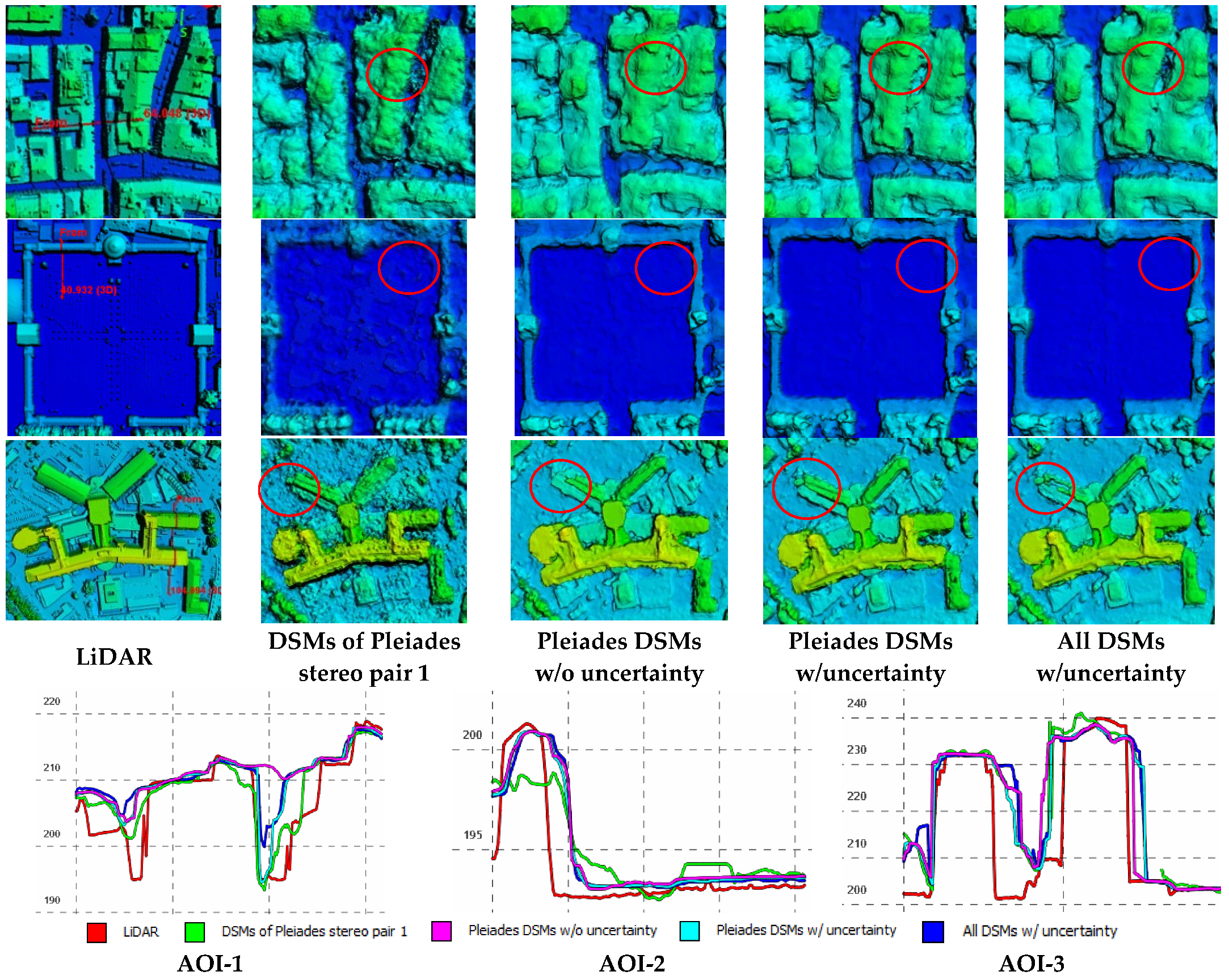
4.2. Accuracy Assessment

The proposed fusion algorithm works at the polynomial complexity (Algorithm 1). It was implemented to allow operational-level reconstruction for the entire area of the test field. For example, using the Pleiades triplet, the 3D reconstruction process over the 400 km² at 0.5 m GSD using a Xeon w2275 (14 cores, 3.30 GHZ) machine with approximately 24 GB of peak memory took approximately 5.5 h for the DSM generation and approximately 1.5 h to fuse the three DSMs (Figure 5).

To quantitatively assess the accuracy of the generated DSMs, we co-registered the photogrammetric results to the reference LiDAR DSM and computed the mean, standard deviation (STD) of the height residuals, and the root-mean-squared errors (RMSE) against the LiDAR DSM. The co-registration was performed through a simplified least-squares surface matching [27] using an affine transformation between the two DSMs.

Table 2. Accuracy statistics (in meters) of individual and fused DSMs with respect to LiDAR DSM. The best results of each column for each AOI region are in bold.

Generated DSMs	AOI-1			AOI-2			AOI-3
	Mean	STD	RMSE	Mean	STD	RMSE	Mean	STD	RMSE
Pleiades stereo pair 1 (int. ang. 5.57°)	0.92	4.04	4.14	0.89	3.02	3.15	1.67	3.56	3.93
Pleiades stereo pair 2 (int. ang. 27.85°)	1.75	4.00	4.36	1.03	3.08	3.25	1.42	3.74	4.00
Pleiades stereo pair 3 (int. ang. 33.42°)	1.61	4.22	4.52	0.84	3.26	3.37	1.55	3.80	4.11
GeoEye-1 stereo pair (int. ang. 30.30°)	1.26	4.15	4.34	0.48	3.03	3.07	1.32	3.71	3.93
WorldView-2 stereo pair (int. ang. 33.71°)	2.01	4.40	4.84	1.47	3.39	3.70	2.22	4.26	4.80
Fused Pleiades pairs w/uncertainty (ours)	1.48	3.80	4.08	0.89	2.92	3.05	1.46	3.46	3.75
Fused Pleiades pairs w/o uncertainty	1.62	4.01	4.32	0.86	2.93	3.06	1.14	3.61	3.79
Fused all pairs w/uncertainty (ours)	1.49	3.90	4.17	0.87	2.86	3.00	1.54	3.49	3.82
Fused all pairs w/o uncertainty	1.49	3.98	4.25	0.82	2.90	3.01	1.23	3.60	3.81

lists the accuracy statistics of the comparisons of the various pair and fusion configurations. We noted that “Pleiades pair 1” with a very small convergence angle (5.57°) achieved the best result among the results from single pairs. This is in line with conclusions noted by a few existing works [4,11,23] that stereo pairs with smaller intersection angles tend to produce DSMs with small RMSE, primarily due to their ability to reconstruct detailed urban structures. In addition, our fusion results achieved the best RMSE for all the AOIs. For AOI-2 and 3, using the Pleiades DSMs alone, we achieved slightly lower RMSE than when using all DSMs. For AOI-2, using all DSMs, we achieved slightly lower RMSE. In a recent publication [28], the authors evaluated the entire region (including flat and hilly regions) using the very same Pleiades triplet, and they only achieved a 5 m RMSE using the Pleiades stereo pair 1, while they achieved RMSE values of 3.2 and 3.4 m for the other two pairs. It should be noted that the entire test region has more flat areas and building-free regions where the accuracy can benefit from stereo pairs with large intersection angles (e.g., Pleiades stereo pairs 2 and 3).

Among all the RMSE values of different pair and fusion configurations, the best RMSEs were achieved by the proposed uncertainty-guided fusion method (whether on the Pleiades DSMs or all DSMs). Note that in AOI-1 and AOI-3, the RMSEs of uncertainty-guided fusion on the Pleiades pairs alone were slightly lower than those using all the five pairs. Since both AOI-1 and 3 contain dense buildings and narrow streets, this might have been due to the fact that DSMs generated by the other two pairs (GeoEye1 and WorldView2) may have failed to reconstruct the topography of the narrow streets; thus, it might negatively impact the final fused DSM if they were considered. However, for fusion without uncertainty metrics, the RMSE followed the intuitive expectation that the more DSMs are used, the lower the achieved RMSE will be. This indicates that our proposed uncertainty-guided fusion approach can explore information with fewer DSMs to achieve higher accuracy.

In addition, the accuracies of different DSMs were evaluated using just building objects (Figure 6), as an important application of these VHR DSMs is to perform LoD1 or LoD2 building/object modeling [29].

Table 3. Accuracy statistics (meter) of individual DSMs and the fused DSMs over rooftops. The best results of each column for each AOI region are in bold.

Generated DSMs	AOI-1			AOI-2			AOI-3
	Mean	STD	RMSE	Mean	STD	RMSE	Mean	STD	RMSE
Pleiades stereo pair 1 (int. ang. 5.57°)	−0.17	2.27	2.28	−0.35	1.94	1.97	−0.46	2.52	2.56
Pleiades stereo pair 2 (int. ang. 27.85°)	0.69	2.10	2.21	0.50	1.74	1.81	−0.12	2.70	2.71
Pleiades stereo pair 3 (int. ang. 33.42°)	0.51	2.28	2.33	0.23	2.01	2.02	−0.02	2.62	2.62
GeoEye-1 stereo pair (int. ang. 30.30°)	0.11	2.23	2.23	−0.08	1.64	1.64	−0.28	2.27	2.28
WorldView-2 stereo pair (int. ang. 33.71°)	0.64	2.44	2.52	0.66	1.92	2.03	0.23	2.95	2.96
Fusion Pleiades pairs w/uncertainty (ours)	0.44	2.04	2.09	0.26	1.61	1.64	−0.12	2.33	2.33
Fusion Pleiades pairs w/o uncertainty	0.50	2.09	2.15	0.31	1.69	1.72	−0.60	3.06	3.12
Fusion all pairs w/uncertainty (ours)	0.28	2.06	2.08	0.16	1.58	1.59	−0.17	2.20	2.21
Fusion all pairs w/o uncertainty	0.29	2.05	2.07	0.17	1.59	1.60	−0.57	2.87	2.92

lists the accuracy statistics of this assessment. The result showed similar conclusions to the overall assessment (Table 2), with the proposed method reaching overall better results, in particular through the fusion of all DSMs. By comparing the accuracy statistics for DSMs produced by fusion with and without uncertainty metrics in Table 3, we found that our proposed method achieved only a marginal improvement. In AOI-1, fusions with and without uncertainty over all the DSMs achieved very similar results, which shows that the dense matching in these building objects yielded fewer errors and the fusion results improved as the number of DSMs increased.

Figure 7 shows three enlarged views of the DSMs generated under different configurations for fusion (with and without uncertainty guidance). It shows that “Pleiades pair 1” achieved the best results among the single-pair DSMs, while visually it yielded much noisier results than any of the fused DSMs (the readers may focus on the circled regions). Furthermore, for the flat region shown in the central row of Figure 7 (from AOI-2), the fusion results of all pairs generally outperformed the fusion results of the Pleiades tri-stereo data alone. Among these, the proposed fusion method using the Pleiades DSMs alone produced smoother surfaces than the other methods (i.e., those without uncertainty). In the case of large complex buildings (from AOI-3—third row of Figure 7), we observed clear quality differences, shown in the red circle, with the proposed method outperforming the others. Profile analyses against the LiDAR reference data confirmed these achievements.

The proposed uncertainty-guided fusion approach was also compared with a few typical approaches for satellite DSM fusion, namely median filter, adaptive median filter [7], and a clustering-based filtering [2]. It should be noted that the comparative study was based only on scalable approaches that have already been applied on large-format images (i.e., hundreds and thousands of megapixels), while other approaches (including deep-learning-based fusion approaches) that have been developed to process RGB-D fusion were not considered here.

To ensure a fair comparison, images were relatively oriented using RSP software [22] and the experiments performed were all based on the same position parameters. The accuracy statistics of this comparative experiment are listed in

Table 4. Comparative study of different fusion methods based on the Pleiades tri-stereo imagery (m).

Areas/Software	Pleiades Pair 1 (a Single Pair)	Median Filter	Adapt. Median [7]	Facciolo et al. [2]	Proposed
AOI-1/RSP	4.14	4.27	4.32	4.76	4.08
AOI-2/RSP	3.15	3.17	3.06	3.64	3.05
AOI-3/RSP	3.93	3.87	3.79	5.30	3.75
AOI-1/ASP	5.79	5.89	5.88	6.18	N.A.
AOI-2/ASP	4.27	4.41	4.38	4.73	N.A.
AOI-3/ASP	5.46	6.28	6.22	5.95	N.A.

. It should be noted that the employed set of ASP parameters (see Appendix A) might not have been the optimal one, given our limited knowledge about the software. Results show that over the three AOIs, the proposed fusion approach achieved the best results in all AOIs. Note that the method presented in [2] was designed for fusing over fifty DSMs. We also observed that in AOI-1, the DSM from the single pair “Pleiades pair 1” achieved a better RMSE than most of the fusion results, and only the proposed fusion method achieved an improved RMSE. This implies that the uncertainty metrics can adaptively reconstruct individually “good” matches that contribute towards a better DSM, even where there are limited numbers of observations.

Additionally, results from the NASA ASP (Ames Stereo Pipeline) software [30] were considered and reported. Since that ASP did not have the function to generate per-pixel uncertainty metrics, the uncertainty-guided fusion method was not applied for ASP results. The ASP program has many parameters and the computations followed an empirical parameter set as described in Appendix A. The fused results from the NASA ASP had worse performance, arguably due to its unsatisfactory performance on single stereo pairs (Table 4 and Figure 8). The fusion of the DSMs generated by ASP did not improve over the individual DSM from Pleiades pair 1 compared to the other approaches. With the proposed fusion method, which includes uncertainty metrics, we achieved approximately 0.06–0.18 m improvement in RMSE over the three AOIs even with only three DSMs, while especially for AOI-1, other fusion methods failed to improve the accuracy over individual DSMs. As compared to the best individual and fused DSMs from ASP, the proposed fusion method achieved significantly more accurate results (1.2–1.8 m less RMSE).

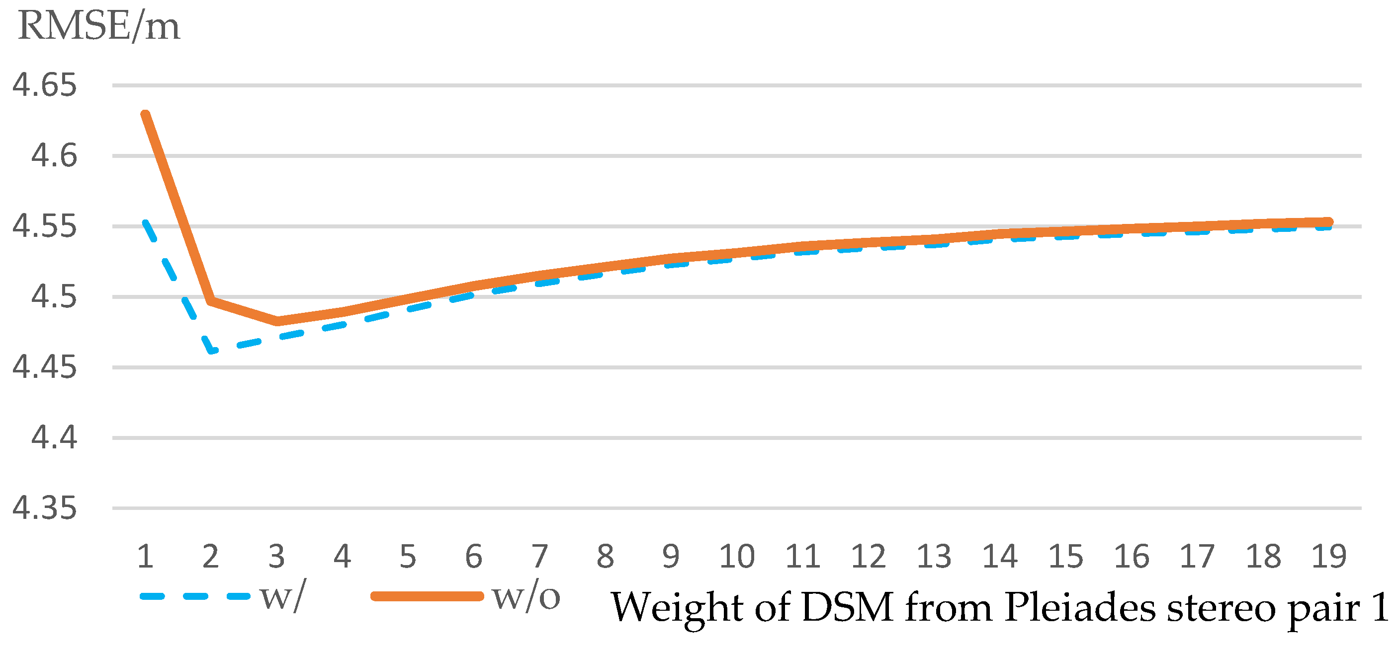
4.3. Weight and Contributions of Individual DSMs in Fusion

Since individual DSMs present different quality (accuracy), we are interested in evaluating how an increased contribution of these “good” DSM may impact fusion results, and whether the increased contribution may further improve the fused result. A simple approach was to repeat these “good” DSMs before fusion. Here, we repeated the DSM generated by “Pleiades stereo pair 1” $N$ times during the fusion, and the results are shown in Figure 9. We observed that different weighting of individual DSMs did show an impact on the final fusion results. The best results were achieved with a certain “$N$”, respectively $N=2$ for fusion with uncertainty, and $N=3$ without uncertainty. Additionally, the fusion with uncertainty metrics achieved the lowest RMSE compared to the fusion without uncertainty.

5. Discussions

The proposed depth-fusion method and the comparative evaluation using various experimental configurations and state-of-the-art fusion algorithms showed that the proposed algorithm achieved favorable RMSE in all tested regions and scenarios. The test regions were selected mostly in the center of Trento, with very complex urban morphology consisting of tall buildings and narrow streets (e.g., as narrow as 5 m in width). We demonstrated that our proposed algorithm achieved an RMSE of 3–4 m in test regions with a Pleiades tri-stereo product, while a previous study using a pair from this dataset achieved a less favorable RMSE of 6.1 m [25]. Our additional evaluation of the accuracy of the building objects showed that the proposed method achieved an RMSE of 1.6–2.1 m.

The experiments and accuracy assessment described in the present paper included DSMs generated through different configurations: (1) individual stereo pairs, (2) fused DSMs using the Pleiades products with and without uncertainty guidance, and (3) fused DSMs using all five DSMs (three Pleiades DSMs, one GeoEye DSM, and one WorldView DSM). This led to the following observations and discussions:

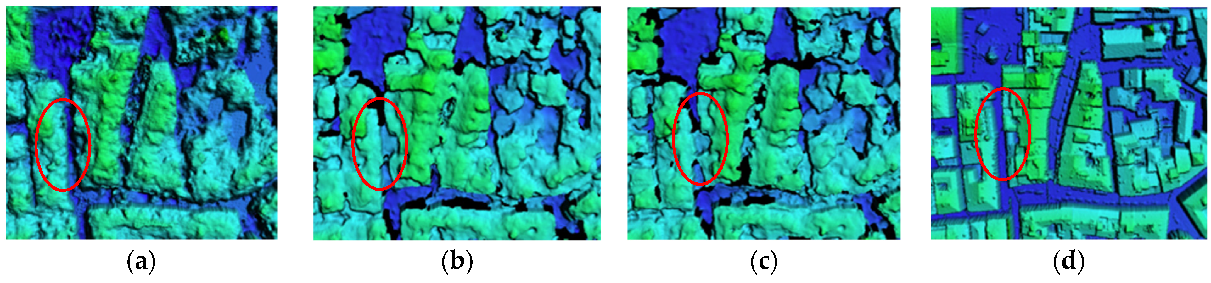
• Sometimes the RMSE of a single pair (e.g., Pleiades pair 1, in AOI-1, Table 4) tended to be better (lower) than that of a fused DSM (using a median filter) in the test regions, primarily due to it being a pair with a very small intersection angle that could pick up narrow streets while others could not. Our proposed algorithm can optimally and adaptively incorporate information of these individual DSMs, and produced a fused DSM better than that of “Pleiades pair 1”;
• Deep and high-frequency relief differences, as shown in the city center areas, remain to be challenging for satellite-based (high-altitude) mapping. Our accuracy analysis showed that the overall RMSE did not necessarily become better as the number of DSMs increased (Table 2), primarily due to the large error rate occurring on the borders of objects and narrow streets; there was only one DSM that reconstructed these deep relief variations correctly (with a very small intersection angle). For building objects that appeared to be nearer objects than the deep and narrow streets, the accuracy followed the intuitive expectation that the RMSE became lower as the number of DSMs increased;
• We considered weighting the contributions of the individual DSMs (Section 4.3), showing that the results of the fusion could be further enhanced by appropriately weighting DSMs of better quality in the fusion procedure. There may be an optimal weight available, although we did not explore further how such a weight might be determined as this exceeded the scope of the current study.

6. Conclusions

This paper proposed a novel depth fusion algorithm for very-high-resolution (VHR) satellite MVS DSMs, which takes into consideration the uncertainty generated during the stereo matching process. The proposed algorithm adopts a simple extension of an adaptive median filter [7]. It includes the per-pixel MVS uncertainties as cues to rank measurements and cluster such measurements into different sets to determine the fused results. The algorithm applies fusion at the individual pixel level and it can be scaled to process large volumes of data. Experiments were carried out using multiple VHR images over the entire town of Trento, Italy, covering an area of approximately 400 km². The accuracy analysis of three test regions showed that the proposed method outperformed all the compared methods. In addition, the proposed algorithm is quite simple and effective at adopting the uncertainties of stereo matching into the fusion framework, being readily available to enable processing of large volumes of data. Furthermore, the optimal weighting schemes of individual DSMs may be determined through further investigation; therefore, future works will include focused investigations and novel uses of these uncertainty metrics, in order to determine the optimal weightings of individual DSMs.

A supplemental video demonstrating DSM results achieved with the proposed method is available at https://youtu.be/NfyrAj4ARys (accessed on 2 March 2022).

References

- Satellite Sensors and Specifications|Satellite Imaging Corp. Available online: https://www.satimagingcorp.com/satellite-sensors/ (accessed on 14 January 2022).
- Facciolo, G.; De Franchis, C.; Meinhardt-Llopis, E. Automatic 3D Reconstruction from Multi-Date Satellite Images. In Proceedings of the IEEE Conference on Computer Vision and Pattern Recognition Workshops, Honolulu, HI, USA, 21–26 July 2017; pp. 57–66. [Google Scholar]
- Bosch, M.; Kurtz, Z.; Hagstrom, S.; Brown, M. A Multiple View Stereo Benchmark for Satellite Imagery. In Proceedings of the 2016 IEEE Applied Imagery Pattern Recognition Workshop (AIPR), Washington, DC, USA, 18–20 October 2016; IEEE: Piscataway, NJ, USA, 2016; pp. 1–9. [Google Scholar]
- Qin, R. A Critical Analysis of Satellite Stereo Pairs for Digital Surface Model Generation and a Matching Quality Prediction Model. ISPRS J. Photogramm. Remote Sens. 2019, 154, 139–150. [Google Scholar] [CrossRef]
- Zhang, K.; Snavely, N.; Sun, J. Leveraging Vision Reconstruction Pipelines for Satellite Imagery. In Proceedings of the IEEE/CVF International Conference on Computer Vision Workshops, Seoul, Korea, 27–28 October 2019. [Google Scholar]
- Zhang, L. Automatic Digital Surface Model (DSM) Generation from Linear Array Images; ETH Zurich: Zurich, Switerland, 2005. [Google Scholar]
- Qin, R. Automated 3D Recovery from Very High Resolution Multi-View Images Overview of 3D Recovery from Multi-View Satellite Images. In Proceedings of the ASPRS Conference (IGTF) 2017, Baltimore, MD, USA, 12–17 March 2017; pp. 12–16. [Google Scholar]
- Huang, X.; Qin, R. Multi-View Large-Scale Bundle Adjustment Method for High-Resolution Satellite Images. arXiv 2019, arXiv:1905.09152. [Google Scholar]
- Bhushan, S.; Shean, D.; Alexandrov, O.; Henderson, S. Automated Digital Elevation Model (DEM) Generation from Very-High-Resolution Planet SkySat Triplet Stereo and Video Imagery. ISPRS J. Photogramm. Remote Sens. 2021, 173, 151–165. [Google Scholar] [CrossRef]
- IARPA Multi-View Stereo 3D Mapping Challenge. Available online: https://www.iarpa.gov/challenges/3dchallenge.html (accessed on 2 March 2022).
- Krauß, T.; d’Angelo, P.; Wendt, L. Cross-Track Satellite Stereo for 3D Modelling of Urban Areas. Eur. J. Remote Sens. 2019, 52, 89–98. [Google Scholar] [CrossRef] [Green Version]
- Albanwan, H.; Qin, R. Enhancement of Depth Map by Fusion Using Adaptive and Semantic-Guided Spatiotemporal Filtering. ISPRS Ann. Photogramm. Remote Sens. Spat. Inf. Sci. 2020, 3, 227–232. [Google Scholar] [CrossRef]
- Yang, J.; Li, D.; Waslander, S.L. Probabilistic Multi-View Fusion of Active Stereo Depth Maps for Robotic Bin-Picking. IEEE Robot. Autom. Lett. 2021, 6, 4472–4479. [Google Scholar] [CrossRef]
- Chen, J.; Bautembach, D.; Izadi, S. Scalable Real-Time Volumetric Surface Reconstruction. ACM Trans. Graph. (ToG) 2013, 32, 1–16. [Google Scholar] [CrossRef]
- Hou, Y.; Kannala, J.; Solin, A. Multi-View Stereo by Temporal Nonparametric Fusion. In Proceedings of the IEEE/CVF International Conference on Computer Vision, Seoul, Korea, 27–28 October 2019; pp. 2651–2660. [Google Scholar]
- Kuhn, A.; Hirschmüller, H.; Mayer, H. Multi-Resolution Range Data Fusion for Multi-View Stereo Reconstruction. In Proceedings of the German Conference on Pattern Recognition, Saarbrücken, Germany, 3–6 September 2013; Springer: Berlin/Heidelberg, Germany, 2013; pp. 41–50. [Google Scholar]
- Rothermel, M.; Haala, N.; Fritsch, D. A median-based depthmap fusion strategy for the generation of oriented points. In Proceedings of the ISPRS Annals of Photogrammetry, Remote Sensing & Spatial Information Sciences, Prague, Czech Republic, 12–19 July 2016; Elsevier: Amsterdam, The Netherlands; pp. 115–122. [Google Scholar]
- Rumpler, M.; Wendel, A.; Bischof, H. Probabilistic Range Image Integration for DSM and True-Orthophoto Generation. In Proceedings of the Scandinavian Conference on Image Analysis, Espoo, Finland, 17–20 June 2013; Springer: Berlin/Heidelberg, Germany, 2013; pp. 533–544. [Google Scholar]
- Unger, C.; Wahl, E.; Sturm, P.; Ilic, S. Probabilistic Disparity Fusion for Real-Time Motion-Stereo. In Proceedings of the ACCV, Queenstown, New Zealand, 8–12 November 2010; Springer: Berlin/Heidelberg, Germany, 2010. [Google Scholar]
- Zhao, F.; Huang, Q.; Gao, W. Image Matching by Normalized Cross-Correlation. In Proceedings of the 2006 IEEE International Conference on Acoustics Speech and Signal Processing Proceedings, Toulouse, France, 14–19 May 2006; IEEE: Piscataway, NJ, USA, 2006; Volume 2, pp. 729–732. [Google Scholar]
- Hirschmuller, H. Accurate and Efficient Stereo Processing by Semi-Global Matching and Mutual Information. In Proceedings of the 2005 IEEE Computer Society Conference on Computer Vision and Pattern Recognition (CVPR’05), San Diego, CA, USA, 20–26 June 2005; IEEE: Piscataway, NJ, USA, 2005; Volume 2, pp. 807–814. [Google Scholar]
- Qin, R. Rpc Stereo Processor (RSP)–a Software Package for Digital Surface Model and Orthophoto Generation from Satellite Stereo Imagery. Int. Arch. Photogramm. Remote Sens. Spat. Inf. Sci. 2016, 3, 77. [Google Scholar]
- Zabih, R.; Woodfill, J. Non-Parametric Local Transforms for Computing Visual Correspondence. In Proceedings of the European conference on computer vision, Stockholm, Sweden, 2–6 May 1994; Springer: Berlin/Heidelberg, Germany, 1994; pp. 151–158. [Google Scholar]
- Rothermel, M.; Wenzel, K.; Fritsch, D.; Haala, N. SURE: Photogrammetric Surface Reconstruction from Imagery. In Proceedings of the Proceedings LC3D Workshop, Berlin, Germany, 4–5 December 2012; Volume 8. [Google Scholar]
- Poli, D.; Remondino, F.; Angiuli, E.; Agugiaro, G. Evaluation of Pleiades-1a Triplet on Trento Testfield. Int. Arch. Photogramm. Remote Sens. Spat. Inf. Sci. 2013, 40, 287–292. [Google Scholar] [CrossRef] [Green Version]
- Agugiaro, G.; Poli, D.; Remondino, F. Testfield Trento: Geometric Evaluation of Very High Resolution Satellite Imagery. Int. Arch. Photogramm. Remote Sens. Spat. Inf. Sci 2012, 39, B8. [Google Scholar] [CrossRef] [Green Version]
- Akca, D. Co-Registration of Surfaces by 3D Least Squares Matching. Photogramm. Eng. Remote Sens. 2010, 76, 307–318. [Google Scholar] [CrossRef] [Green Version]
- Lastilla, L.; Belloni, V.; Ravanelli, R.; Crespi, M. DSM Generation from Single and Cross-Sensor Multi-View Satellite Images Using the New Agisoft Metashape: The Case Studies of Trento and Matera (Italy). Remote Sens. 2021, 13, 593. [Google Scholar] [CrossRef]
- Partovi, T.; Fraundorfer, F.; Bahmanyar, R.; Huang, H.; Reinartz, P. Automatic 3-d Building Model Reconstruction from Very High Resolution Stereo Satellite Imagery. Remote Sens. 2019, 11, 1660. [Google Scholar] [CrossRef] [Green Version]
- Beyer, R.A.; Alexandrov, O.; McMichael, S. The Ames Stereo Pipeline: NASA’s Open Source Software for Deriving and Processing Terrain Data. Earth Space Sci. 2018, 5, 537–548. [Google Scholar] [CrossRef]