Improvement of Lithological Mapping Using Discrete Wavelet Transformation from Sentinel-1 SAR Data

Abstract

Lithological mapping using dual-polarization synthetic aperture radar (SAR) data is limited by the low classification accuracy. In this study, we extract ten parameters (backscatter coefficients and polarization decomposition parameters) from the Sentinel-1 dual-pol SAR data. Using 94 mother wavelet functions (MF), a one-level two-dimensional discrete wavelet transform (DWT) is applied to all the parameters, and the suitable MF is screened by comparing the overall accuracy and F1 score. Finally, the lithological mapping of the study area is performed. According to the cross-validation results, DWT can improve the overall accuracy for all MF. Db13 improved the overall accuracy by 6.1% (from 49.5% to 55.6%). The F1 score of granitoids improved by 0.223. Among the five rock units, Grantoids and Quaternary alluvium and sediment with finer gravel can be better differentiated than the other three rock units. The overall accuracy of effusive rocks (marine basic volcanic rocks) is not improved by DWT, but this study confirms the great potential of DWT in lithology classification.

1. Introduction

Remote sensing has the advantages of a large detection range and fast data acquisition. The use of remote sensing for geological mapping can shorten the production cycle of geological maps. Optical sensors and satellites such as ASTER, Landsat-8, and Sentinel-2 are now widely used for large-scale geological mapping due to the typical characteristic spectral profiles of different rocks or minerals [1,2,3]. Hewson et al. [4] generated maps of carbonate and ferrous iron content from ASTER short-wave infrared (SWIR) data and quartz content from thermal infrared (TIR) data. Almalki et al. [5] used band ratios to highlight differences between bands of Landsat-8 to map the geology of hard-to-reach islands. Albert et al. [6] combined Sentinel-2 and the shuttle radar topography mission (SRTM) digital elevation model (DEM) data to produce geological maps of arid regions. Several studies have used more than one type of optical remote sensing data [7]. Pour et al. [8] used ASTER and Landsat-8 data to map lithology and alteration minerals in Antarctica. Sekandari et al. [9] used band ratios and principal component analysis (PCA) methods to extract Pb–Zn mineralization with multiple optical remote sensing data. Different data provide multiple wavelengths and information related to rocks or minerals.

Synthetic aperture radar (SAR) data are less commonly used for geological mapping. As long wavelength data, SAR provides different texture information and scattering mechanisms than optical sensors. Pour et al. [10] used ASTER data for mineral mapping. PALSAR data were used to detect linear structures (faults and fractures) and curvilinear structures (back-slope and dip). Choe et al. [11] discussed the application of the roughness characteristics provided by SAR data in assisting the geological mapping of ASTER and Landsat-8 data. Pour et al. [12] combined Hyperion and SAR data to enable the identification of hydrothermal alteration rocks by textural variations in outcrop and surface roughness. This is useful for exploring gold mineralization in Malaysia.

Suspended material in the air can affect the imaging of optical sensors, while SAR can penetrate clouds and fog to detect the surface directly. Although SAR has many advantages, rock-type discrimination using SAR data alone is less effective. SAR does not have as many bands as multispectral or hyperspectral sensors, so it is difficult to find parameters that are directly related to rocks or minerals. Lu et al. [13] discussed the capability of Sentinel-1 in lithology discrimination, but only close to half of the samples could be correctly classified. Radford et al. [14] compared the accuracy of SAR, gravity, and magnetic data for rock-type identification and found that gravity and magnetic data with lower resolution had stronger classification capability. The low accuracy of lithology discrimination shown in their studies may make it difficult to use SAR data alone for lithological mapping. Although the overall accuracy is improved by combining SAR with optical remote sensing data, the difference in the imaging time of multiple sensors affected the reproducibility of the conclusions.

Currently, methods to improve the accuracy of rock-type discrimination based on SAR data focus on (i) improvements in classification algorithms (e.g., improvements in deep-learning algorithms) [15], (ii) using time series to filter features [16], and (iii) using multi-frequency or fully polarized data [15,17]. With the development of artificial intelligence, the classification ability of classifiers has gradually improved. Recently, deep learning has been commonly used to improve the classification accuracy of remote sensing data [18,19]. Deep-learning algorithms require a large number of training samples, and many studies do not investigate the sample points in the field but select samples directly based on geological maps. This has a significant impact on the classification effectiveness due to the limited accuracy of the geological map and the fact that it does not show all rock types. Time series are commonly used in crop and sea ice classification [20]. Although rock morphology hardly changes within several years, SAR is very sensitive to surface morphology, and different weather conditions may make rock units differently separable. Lu et al. [16] extracted one year of VV/VH backscatter coefficients from Sentinel-1 images and improved the overall accuracy by 9% compared to a single image. Time series are applicable for open-access data such as Sentinel-1, but for most SAR data, this is costly. More studies have used fully polarized or multi-frequency data for classification [21,22]. Data with different polarizations feed back different scattering mechanisms, which is effective in rock identification. However, the use of multi-frequency SAR may face the same limitation of higher cost.

The dual-pol SAR data has only two bands, and the correlation between adjacent rows or columns of the image is strong, so the information available for extraction is limited. It is a meaningful task to mine as many features as possible from one image. We have used wavelet transform for microwave feature-extraction of rock units. The wavelet transform can send the signal from the spatial domain to the frequency domain with little correlation between the transformed components [23]. The single-dimensional wavelet transform is often used to process vibrational signals and is commonly used in remote sensing to extract features of spectral curves. Yang et al. [24] found that the high-frequency components of the wavelet-transformed spectral curve have a strong correlation with the feldspar content in rocks. Two-dimensional (2D) wavelet transforms are often used for image denoising, compression, or classification [25]. SAR images often contain a lot of speckle noise, and wavelet-based denoising methods are widely used [26,27]. In image classification, the wavelet transform is often used for feature extraction [28,29]. Wavelet-transformed images are better for medical disease diagnosis and land-use classification [30]. 2D discrete wavelet transform (DWT) produces high-frequency and low-frequency components uniquely characterizing the surface texture, which contributes significantly to identifying sea ice using remote-sensing images [31,32]. However, few studies have explored the potential of the 2D wavelet transform for lithological mapping using SAR data. Understanding the performance of different types of mother wavelet functions (MF) in rock-unit classification can help to reduce the experimental time in future studies [33,34,35]. This method does not require multiple images, which improves the classification results while saving costs.

This paper aims to perform the lithological mapping ability of Sentinel-1 in the East Tianshan region of western China with the help of 2D DWT and a random forest classifier. The main objectives of this study are (i) to extract the backscattering features and decomposition features of different types of rock units based on Sentinel-1; (ii) to select the MF that is most suitable for rock type classification; and (iii) to accurately verify and robustly check the different temporal data.

2. Study Area and Data

2.1. Study Area and Samples

The study area is located in the eastern part of the East Tianshan Mountains of China. The region is hot and arid in summer, with few anthropic settlements and sparse vegetation [36]. As part of the Great South Lake coal mining area, the area contains abundant coal deposits.

The samples are derived from the results of the fieldwork in 2020 (Figure 1). Each sample we recorded has a size of about 50 m × 50 m. To maintain accuracy while combining the 10 m resolution of Sentinel-1, each sample area was finally set to 30 m × 30 m. The geological map shows that the lithology of the study area includes medium basal igneous rocks, pyroclastic rocks, albite porphyry, mudstone, sandstone, and granite (Figure 2) [37]. During the fieldwork, the igneous rocks were visually discernible. However, much of the bedrock may not have been exposed at the surface or may have been heavily fractured during weathering.

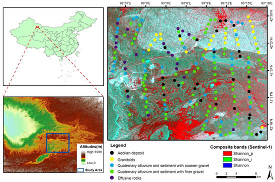
Figure 1. Distribution of samples in the study area. The background image is Shannon entropy extracted from Sentinel-1. Elevation data are derived from the shuttle radar topography mission (SRTM).

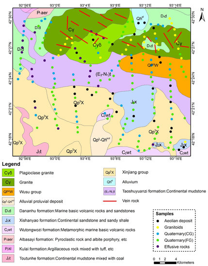
Figure 2. Geological map of the study area. The scale of mapping format is 1:500,000.

Due to the limited penetration ability of SAR data, we used the rock types exposed to the surface as the classification criterion. According to the record results of fieldwork, the rock unit types in the study area mainly include granitoids, effusive rocks, aeolian deposits, Quaternary alluvium and sediment with coarser gravel, and Quaternary alluvium and sediment with finer gravel. Since it is not easy to distinguish granite and granitic amphibolite in the field, we uniformly named them granitoids. For alluvium and sediments, we use the size of gravel to distinguish them. Those with gravel sizes in the range of 1–5 cm are classified as Quaternary alluvium and sediment with finer gravel, while those with gravel sizes in the range of 5–30 cm are classified as Quaternary alluvium and sediment with coarser gravel. Table 1 shows the rock unit types and their properties.

Table 1. Rock unit types, field photos, and lithology in the geological map.

Rock Unit Types	Abbreviations	Field Photos	Lithology from the Geological Map
Aeolian deposits	Aeolian deposits		Alluvial proluvial deposit
Granitoids	Granitoids		Plagioclase granite and granite
Quaternary alluvium and sediment with coarser gravel	Quaternary (CG)		Usu group and Xishangyao formation
Quaternary alluvium and sediment with finer gravel	Quaternary (FG)		Xinjiang group and Taoshuyuanzi formation
Effusive rocks	Effusive rocks		Dananhu formation and Wutongwozi formation

2.2. Data

In this study, we used 14 Sentinel-1 single-look complex (SLC) with the polarization VV and VH. All data were imaged from July to September to avoid moisture interference. Among them, one image was used for screening the appropriate MF and lithological mapping. It was imaged on 20 August 2020. Thirteen images were used to verify the robustness of the results to the angle of incidence. All data used in the experiments are shown in Table 2.

Table 2. All Sentinel-1 SAR data were involved in the study.

Experimental-Data Imaging Date	Verification-Data Imaging Date
20 August 2020	3 July 2020
	8 July 2020
	15 July 2020
	20 July 2020
	27 July 2020
	1 August 2020
	13 August 2020
	25 August 2020
	1 September 2020
	6 September 2020
	13 September 2020
	18 September 2020
	25 September 2020

3. Methodology

The method mainly consists of four parts:

(1) The preprocessing of SAR data: the extraction of polarization decomposition parameters and backscatter coefficients;

(2) 2D-DWT of the parameters;

(3) Random forest classification, the selection of MF, and a robustness test;

(4) Lithological mapping and the analysis of classification results.

3.1. Preprocessing of Sentinel-1 and Parameter Extraction

Preprocessing of Sentinel-1 and parameter extraction were implemented in Sentinel’s Application Platform (SNAP) from ESA and PolSARpro v5.1.3 [38,39]. PolSARpro v5.1.3 was developed by the Institute of Electronics and Telecommunications of Rennes of the University of Rennes 1 (Rennes, France). The extraction process of scattering parameters (backscatter coefficients) contains orbit correction, radiometric calibration, deburst, multilooking, speckle filtering, and terrain correction. The extraction process of the polarization decomposition parameters (H, A, α, Shannon entropy, λ1, and λ2) generates the complex matrix during radiometric calibration and implements the final decomposition in PolSARpro v5.1.3 [40,41]. The filter is selected as the Refined LEE filter, and the DEM used for terrain correction is the SRTM DEM [42]. Figure 3 shows the flow chart of preprocessing. The ten parameters extracted from Sentinel-1 are shown in Table 3. They describe the scattering mechanisms for different rock types.

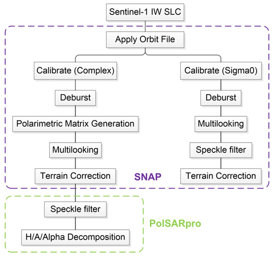
Figure 3. Flow chart of SAR data preprocessing and parameter extraction.

Table 3. SAR parameters extracted in this study.

Features	Bands (Abbreviations)
Backscatter coefficients	Backscatter coefficient of VV (Sigma0_VV)
	Backscatter coefficient of VH (Sigma0_VH)
Polarization decomposition parameters	Entropy (H)
	Alpha (α)
	Anisotropy (A)
	Shannon entropy (Shannon)
	Shannon-entropy intensity component (Shannon_i)
	Shannon-entropy polarization component (Shannon_p)
	Eigenvalue 1 of the polarization covariance matrix (λ1)
	Eigenvalue 2 of the polarization covariance matrix (λ2)

3.2. Discrete Wavelet Transform

The wavelet transform is an ideal tool for signal time-frequency analysis [23]. The schematic diagram of the 2D-DWT is shown in Figure 4. The 2D-DWT deals with a 2D numerical discrete matrix, and the process of wavelet transformation includes wavelet decomposition and reconstruction. Each decomposition produces one low-frequency component (A) and three high-frequency components (horizontal (H), vertical (V), and diagonal (D)). The high-frequency component shows the image edges or noise, i.e., the areas where the grayscale values change sharply. The low-frequency information is the area where the grayscale changes slowly.

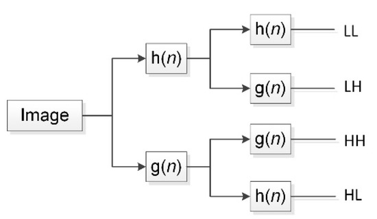
Figure 4. Decomposition of 2D-DWT.

DWT in this study was implemented in the wavelet toolbox of Matlab R2021b, which was developed by The MathWorks Inc. (Natick, MA, USA) [43,44]. Usually, the selection of MF requires continuous attempts to finally select the most suitable MF. We selected MF with both double orthogonality and discrete properties. The Daubechies series, Symlet series, and Coiflet series wavelets were used to implement wavelet decomposition and reconstruction. Table 4 shows the MF used in this study.

Table 4. All MF used in this study.

Mother Functions (MF)	Abbreviations of Mother Functions
Daubechies	db1, db2…db45
Symlet	sym2, sym3…sym45
Coiflet	coif1, coif2…coif5

For each MF, we performed one-level decomposition and reconstruction for all parameters extracted from Sentinel-1, i.e., each image is transformed into four images. Even though DWT can carry out multi-level decomposition, only one level of decomposition is performed in this study due to the large number of MF.

3.3. Rock-Type Descriptors

μ and l2 were used to describe the regional characteristics of each sample in the image with the following equations [45]:

$$\mu =\frac{1}{M\times N}{\displaystyle \sum _{k=1}^M{\displaystyle \sum _{i=1}^N}}|f(x,y)|$$

(1)

$$l2=\frac{1}{M\times N}{\displaystyle \sum _{k=1}^M{\displaystyle \sum _{i=1}^N}}{[f(x,y)]}^2$$

(2)

These descriptors are computed in all the sample regions, where M denotes the number of columns of each sample matrix, N denotes the number of rows of each sample matrix, and f (x,y) denotes the sample matrix.

3.4. Kruskal–Wallis Test

The Kruskal–Wallis (K–W) test was performed on all of the samples to explore the differences in the parameters after DWT and the ability to distinguish between different rock types [34]. The results of the K–W test were combined with the accuracy of the classifier and used together as an evaluation criterion for classification effectiveness.

3.5. Evaluation of the Classification Accuracy and the Selection of MF

The random forest (RF) method was used to classify rock types. In the process of screening MF, 5-fold cross-validation tests were used to evaluate the classification performance. The RF algorithm used the package randomForest in R 4.0.5, developed by Andy Liaw and Matthew Wiener (Rahway, NJ, USA) [46]. Overall accuracy, KAPPA coefficients, and F1 score were used to evaluate the classification effectiveness. These metrics evaluate the ability of different MF to improve the classification of rock units from both overall and category perspectives. Because of the differences between the metrics, we combined all of the metrics and selected the excellent MF.

The incidence angle of SAR may affect the final result. To demonstrate the robustness of the MF with great performance to the incidence angle, we selected 13 summer season images. The classification was performed separately using the original SAR parameters and the parameters based on DWT. It was observed whether the overall accuracy was improved after DWT.

3.6. Lithological Mapping

All pixels in the study area are classified using the parameters extracted from the optimal MF. Finally, the resulting map is compared with the geological map and Sentinel-2 data to analyze and summarize the advantages and disadvantages of lithological mapping using SAR data.

4. Results

4.1. Extraction of Sentinel-1 Parameters

Backscatter coefficients and decomposition parameters were extracted. Figure 5 shows the VV and VH polarization backscatter coefficients imaged on 8 August 2020. The brown line in the figure is the geological boundary in the geological map. The boundaries on the northern sector of the study area are in good agreement with the geological map boundaries. In general, the trend of the backscatter coefficient is in agreement with the boundary line in the geological map.

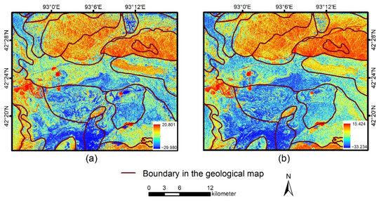
Figure 5. Backscatter coefficients extracted from Sentinel-1 collected on 8 August 2020: (a) results of VV polarization and (b) results of VH polarization.

4.2. Selection of MF

In the ranking of the overall accuracy of RF (Table 5), db19, db34, db4, db26, and db13 are the top five MF. Db19 has the highest overall accuracy of 0.570 and a KAPPA coefficient of 0.356. The overall accuracy without DWT is 0.495, ranking 92nd. Db19 improves the overall accuracy by 7.5% and the KAPPA coefficient by 0.095. All MF have a positive effect on improving classification accuracy. Regardless of the MF used for DWT, the overall accuracy is no less than the accuracy of the original parameters. It is worth mentioning that the top ten MF in terms of overall accuracy are all Daubechies series functions.

Table 5. Overall accuracy and KAPPA coefficients of different MF (ranked in terms of overall accuracy).

Ranking	MF	OA	KAPPA	Ranking	MF	OA	KAPPA
1	db19	0.570	0.356	49	sym38	0.530	0.298
2	db34	0.565	0.348	50	db8	0.530	0.297
3	db4	0.560	0.350	51	db14	0.530	0.298
4	db26	0.559	0.338	52	db23	0.530	0.299
5	db13	0.556	0.340	53	db32	0.530	0.301
6	db10	0.555	0.338	54	db39	0.530	0.299
7	db41	0.555	0.334	55	sym27	0.530	0.296
8	db11	0.555	0.335	56	sym31	0.530	0.297
9	db33	0.551	0.327	57	db36	0.530	0.290
10	db40	0.551	0.330	58	sym16	0.526	0.287
11	coif5	0.551	0.331	59	sym36	0.526	0.286
12	db27	0.550	0.324	60	sym14	0.526	0.289
13	db18	0.550	0.326	61	sym22	0.526	0.292
14	coif2	0.546	0.324	62	sym39	0.525	0.289
15	sym18	0.546	0.318	63	sym42	0.525	0.285
16	db45	0.546	0.317	64	db15	0.525	0.290
17	db20	0.545	0.318	65	sym34	0.525	0.289
18	sym35	0.545	0.317	66	db5	0.525	0.289
19	sym43	0.545	0.325	67	sym24	0.525	0.288
20	db12	0.545	0.319	68	db3	0.525	0.291
21	db16	0.545	0.321	69	db29	0.525	0.284
22	db17	0.545	0.321	70	db38	0.525	0.288
23	db28	0.545	0.317	71	sym23	0.525	0.297
24	db1	0.545	0.327	72	sym32	0.521	0.281
25	sym19	0.545	0.321	73	sym2	0.520	0.276
26	db43	0.545	0.320	74	sym25	0.520	0.276
27	sym11	0.545	0.321	75	sym40	0.520	0.282
28	sym15	0.545	0.319	76	sym44	0.520	0.279
29	db42	0.545	0.321	77	db7	0.520	0.287
30	db30	0.541	0.311	78	sym26	0.520	0.281
31	sym8	0.540	0.306	79	sym6	0.520	0.283
32	coif3	0.540	0.316	80	db31	0.516	0.267
33	sym30	0.540	0.315	81	db24	0.515	0.271
34	db6	0.540	0.314	82	sym37	0.515	0.272
35	coif4	0.540	0.314	83	sym3	0.515	0.275
36	db35	0.540	0.315	84	sym12	0.511	0.265
37	sym7	0.540	0.316	85	sym20	0.511	0.267
38	db44	0.540	0.312	86	sym4	0.511	0.276
39	db22	0.536	0.304	87	db2	0.510	0.261
40	sym28	0.535	0.302	88	sym41	0.510	0.260
41	db21	0.535	0.299	89	sym29	0.505	0.256
42	coif1	0.535	0.313	90	sym33	0.505	0.256
43	sym10	0.535	0.302	91	sym21	0.500	0.252
44	db25	0.535	0.310	92	original	0.495	0.261
45	db37	0.535	0.302	93	sym17	0.495	0.248
46	sym5	0.531	0.298	94	db9	0.495	0.243
47	sym9	0.530	0.298	95	sym45	0.495	0.243
48	sym13	0.530	0.296

We counted the highest F1 score corresponding to each rock unit (Table 6). The highest F1 score of the aeolian deposit, granitoids, quaternary (CG), and quaternary (FG) were all from the Daubechies series functions. The highest F1 score is from quaternary (FG) at 0.693, and the lowest F1 score is from effusive rocks at 0.080. Compared with the F1 score of the original parametric classification, the F1 score of granitoids improved the most after DWT. The F1 score of granitoids was improved from 0.480 to 0.703. Even with DWT, the accuracy of effusive rocks was still not optimistic.

Table 6. The highest value of F1 score among the rock units on Sentinel-1 data using DWT.

Rock Unit Types	MF	Precision	Recall	F1 Score	Original F1 Score	Original F1 Score Ranking
Aeolian deposit	db34	0.7	0.167	0.264	0.241	9
Granitoids	db34	0.655	0.78	0.703	0.480	95
Quaternary (CG)	db19	0.526	0.511	0.507	0.411	48
Quaternary (FG)	db19	0.589	0.847	0.693	0.648	75
Effusive rocks	db13	0.2	0.05	0.08	0.057	7
	db35	0.2	0.05	0.08
	coif3	0.2	0.05	0.08
	coif4	0.2	0.05	0.08

Combining the overall accuracy and F1 score, db19, db34, and db13 performed the best. We found that the discrimination ability of the effusive rocks was generally low. db19 and db34 cannot correctly identify any effusive rocks. Considering the F1 score of effusive rocks, finally, we chose db13 as the suitable MF for this lithological mapping. The precision, recall, F1 score, and F1 score ranking of various rock units after DWT (MF: db13) are shown in Table 7.

Table 7. Classification accuracy of various rock types corresponding to db13.

Rock Unit Types	Precision	Recall	F1 Score	F1 Score Ranking
Aeolian deposit	0.6	0.133	0.214	32
Granitoids	0.559	0.69	0.610	84
Quaternary (CG)	0.495	0.461	0.473	7
Quaternary (FG)	0.586	0.824	0.682	7
Effusive rocks	0.2	0.05	0.08	1

4.3. K–W Test of the Samples

Table A1 in Appendix A shows the results of the K–W test for all parameters used for classification. Table 8 shows the p-value of the original parameters and the low-frequency components after DWT. When the p-value is less than 0.05, the samples are considered to be statistically different from each other. For most parameters, the p-value decreased after DWT, which indicates that the wavelet transform enhances the separability between different rock units.

Table 8. p-value of the original parameters and the low-frequency components after DWT. Letter A after the parameter indicates the low-frequency component after DWT.

Parameters	p-Value of Parameters after DWT	p-Value of Original Parameters
Sigma0_VH_μ_A	2.31 × 10−13	8.35 × 10−13
Sigma0_VV_μ_A	5.82 × 10−13	9.77 × 10−11
A_μ_A	2.10 × 10−2	3.85 × 10−10
α_μ_A	1.28 × 10−2	6.82 × 10−12
H_μ_A	2.11 × 10−2	6.10 × 10−12
Shannon_μ_A	1.68 × 10−13	8.68 × 10−11
Shannon_i_μ_A	2.75 × 10−12	1.09 × 10−2
Shannon_p_μ_A	1.93 × 10−2	1.15 × 10−2
λ1_μ_A	1.38 × 10−11	5.40 × 10−3
λ2_μ_A	5.85 × 10−13	1.17 × 10−2
Sigma0_VH_l2_A	2.23 × 10−13	8.67 × 10−13
Sigma0_VV_l2_A	6.44 × 10−13	1.03 × 10−10
A_l2_A	2.14 × 10−2	3.89 × 10−10
α_l2_A	1.36 × 10−2	7.10 × 10−12
H_l2_A	2.17 × 10−2	5.84 × 10−12
Shannon_l2_A	1.72 × 10−13	8.60 × 10−11
Shannon_i_l2_A	2.80 × 10−12	1.09 × 10−2
Shannon_p_l2_A	1.75 × 10−2	1.18 × 10−2
λ1_l2_A	1.55 × 10−11	5.45 × 10−3
λ2_l2_A	6.98 × 10−13	1.15 × 10−2

4.4. Db13 Wavelet Robustness Test

The parameters of the 13 SAR images were performed with 2D DWT (MF: db13), and the results were compared using the original parameters and the transformed parameters. Among all the data, only the data imaged on 13 August 2020 had worse overall accuracy after DWT than before (Figure 6). The overall accuracy of the remaining 12 data improved by 2–11% after DWT (MF: db13). The accuracy of the wavelet-transformed data (MF: db13) reached more than 0.5 for 7 images.

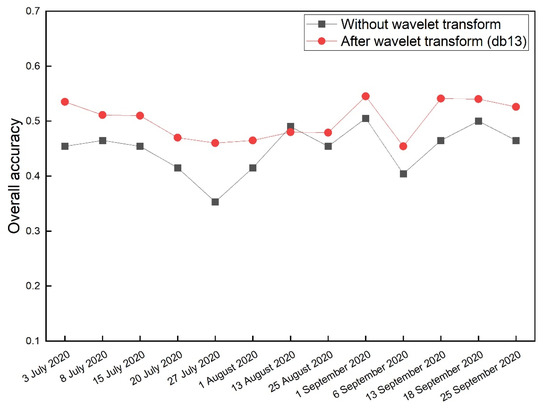
Figure 6. Robustness test results of db13. The horizontal axis represents the imaging date of SAR data, and the vertical axis represents the overall accuracy of the classification.

4.5. Lithological Mapping

Figure 7 shows the results of lithological mapping using the original parameters. Granitoids are mainly developed on the northern sector of the study area, and aeolian deposits are mainly distributed on the southern sector. Quaternary (SG) is distributed in a large area. The boundaries of rock types are relatively clear, but a large number of speckles appear in the image. The buildings and water bodies are misclassified into granitoids and effusive rocks.

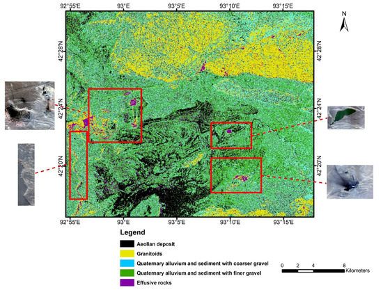
Figure 7. Results of lithological mapping using original parameters. The water body and landmark buildings in the figure are marked with WorldView-2 data© DigitalGlobe, Inc. (Westminster, CO, USA) (2020), provided by European Space Imaging.

Figure 8 shows the classification result after DWT (MF: db13). Compared with Figure 7, Figure 8 has a filter-like effect with clear boundaries. The comprehensive geological map shows that granitoids in the northern sector of the study area are better classified. The buildings and metal facilities in the area are misclassified into granitoids, which is due to their all having relatively high backscatter coefficients. The Quaternary alluvium in the study area is stratified. At locations where elevation changes occur, especially for the geomorphic boundary, alluvium- and sediment-containing gravels are misclassified into granitoids. A large number of well-defined strips of quaternary (CG) occur in the granite bodies in the northern sector of the study area, which are known to be acidic and basal vein rocks on the geological map.

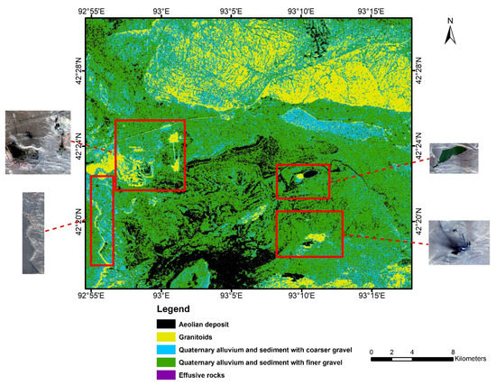
Figure 8. Results of lithological mapping using parameters after DWT (MF: db13). The water body and landmark buildings in the figure are marked with WorldView-2 data© DigitalGlobe, Inc. (Westminster, CO, USA) (2020), provided by European Space Imaging.

From the degree of coincidence with the geological map, the results after DWT are better than those without wavelet transform. Figure 8 has demonstrated the improvements of DWT for larger-scale lithological mapping.

5. Discussion

The principle of lithology classification by optical and TIR remote sensing is that different minerals have typical reflectance or emissivity in different bands. Due to the long wavelength of microwaves, there is no strong correlation between parameters and minerals. The echo intensity of SAR in arid regions is correlated with surface roughness and dielectric constant [47]. Backscatter coefficients, polarization decomposition features, and texture features have been mainly used for lithology classification in previous studies [13]. In many studies, combining SAR data with DEM enhances the accuracy because different rocks have different morphologies, which may lead to different elevations, but this does not capture the ability of SAR data to distinguish rock types. To discuss the contribution of dual-pol SAR data in lithological mapping, we do not use elevation data.

The use of microwave data for lithological mapping is mainly based on the surface morphology of the rock and whether the rock has been mineralized. Nearly half of the study area is within the Gobi Desert, which is heavily weathered. Conversely to optical sensors, the sensitivity to clast sizes makes SAR more suitable for areas of the outcrop of sedimentary clastic rocks.

Unlike many studies that use SAR data for lithology discrimination, we performed lithological mapping after discussing the classification accuracy. This is one of the most important contributions of geology remote sensing. The F1 score of quaternary (CG) after DWT reached 0.682, which is an impressive accuracy in sediment subdivision. The F1-score for granitoids improved by 13% after DWT (MF: db13). However, 57% is not a very satisfactory overall accuracy, mainly because effusive rocks are almost completely unrecognized correctly. After DWT of some MF, effusive rocks are not even correctly identified at all. There are two possible reasons for this: compared with other rock types, the number of effusive rock samples is small. This may lead to the unbalanced classification of the RF classifier. This is a difficult problem to solve because the distribution of rocks on the surface is uneven, and effusive rocks are not marked in many small-scale geological maps. Another possibility is that effusive rocks have similar backscattering characteristics to other rock types. In the future, we will test 2D DWT in the area with clearer outcrops and explore the microwave scattering model of rock.

Most of the boundaries in the wavelet-transformed (MF: db13) classification results of the study area match the geological map. This indicates that one level of DWT can meet the requirements of large-scale lithological mapping. The granite bodies in the northwestern sector of the study area have the most excellent classification quality. There are two possible reasons for the high backscatter coefficients of the granite bodies. Lu et al. [13] tested the dielectric constant of rocks in Xingcheng, China, and we show the dielectric constants of rocks at 5.4 GHz frequency in Table 9. Although granites often have a high dielectric constant, this is not the main reason why they are easy to identify. Rocks in the Gobi and desert often have similar dielectric constants. The dielectric constants of rocks in such a region need to be further studied. Due to the fact the rocks in the study area are scattered as shown in Table 1, the surface roughness may be the main reason for controlling the backscatter coefficients. More roughness experiments will be carried out in future fieldwork. We note that the granite bodies are classified with striated quaternary sediments and alluvium, which are common vein rocks in the study area. During the field investigation, we found that the vein-like distribution of intermediate and acidic rocks (e.g., pegmatites and porphyries) developed in granite and amphibolite areas (Figure 9). Due to only a few vein rock outcrops along the survey route, we did not obtain enough samples, which resulted in different types of vein rocks not being distinguished. Nevertheless, the use of SAR data and DWT for vein-rock identification is a topic that can be explored in depth in the future.

Table 9. Dielectric constants of rocks in other regions at 5.4 GHz frequency [13].

Rock Names	Longitude	Latitude	Dielectric Constant
Brown andesitic crystalline tuff	120.604°E	40.642°N	2.315
Gray-brown andesitic crystalline tuff	120.618°E	40.640°N	2.418
Gravel	120.553°E	40.812°N	2.373
Purple complex-component conglomerate	120.091°E	40.975°N	2.019
Cinereous fine sandstone	120.523°E	40.785°N	4.259
Purple, gravelly siltstone	120.556°E	40.767°N	1.953
Grayish-white granite	120.502°E	40.725°N	5.537
Flesh-red granite	120.749°E	40.840°N	4.400

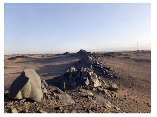
Figure 9. Intermediate rocks are distributed in the diorite area as veins.

Comparing Figure 7 and Figure 8, we can see that the resulting boundary is clearer and smoother after using DWT. These are the most important points to improve the accuracy of the geological map. The low-frequency component of DWT has a filtering effect, which makes the resulting map smoother. The high-frequency component reflects the abrupt change of the signal, which can enhance the detection of the rock-type boundary. Most of the high-frequency components ranked low in the K–W test p-value ranking, which may be due to the small area of each sample, which is not enough to reflect high-frequency components. Obviously, for the classification of the whole study area, the high-frequency components are important. In addition, the ability of vein rocks to be better identified after DWT may be related to the role of the high-frequency components.

Two types of representative features are misclassified: man-made structures on the surface, and locations where significant elevation changes occur. Even though SAR has some penetration ability, it cannot penetrate artificial buildings. In the subsequent process, the surface man-made structures need to be masked off. The boundaries of the folds in the study area and the areas with significant elevation changes were misclassified as granitoids. To some extent, this is a new idea of fold recognition. While previous studies have used spectral information for fold identification, SAR provides roughness information to assist in the identification from another scale. Outside of folds, SAR is often used to identify tectonic phenomena such as faults. We did not perform the identification of faults because the richly developed vein rocks are easily confused with faults in SAR data.

In this study, we performed only one level of DWT. According to the wavelet transform principle, two-level decomposition or higher-level decomposition can yield more variables for classification. Some of the high-frequency components of the one-level decomposition ranked low in the K–W test, and we speculate that some of the components generated by the two-level decomposition may weaken the classification effect. Although the RF classifier is insensitive to features with weak divisibility, we have to consider the fitness of the method for other classifiers.

The traditional method of creating geological maps is to observe the lithology around the geological survey route and delineate similar lithology in the plan. This approach is often less accurate and limited by road conditions. The lithology discrimination method based on 2D DWT and SAR data provided in this study provide a new idea for lithological mapping in arid areas. The wavelet transform technique amplifies the capability of SAR in rock discrimination. Combining DWT with multi-frequency SAR data can be considered in future research to explore a more stable lithological mapping method.

6. Conclusions

Due to the penetrating nature of SAR data, it has been applied to rock-unit classification. However, limited by the low overall accuracy, few studies have directly used dual-pol SAR data for lithological mapping. In this study, we attempt to use DWT to transform the parameters of Sentinel-1 to improve the rock-classification accuracy.

We combined the backscatter coefficients and polarization decomposition parameters extracted from Sentinel-1 and applied the RF algorithm to classify the rock units. All the parameters were decomposed using 94 MF for one level of wavelet decomposition, and the overall accuracy, KAPPA coefficients, and F1 score were used to evaluate the classification effectiveness. The results show that the overall accuracy can be improved regardless of the MF used. Among them, the db13 wavelet has the best improvement for the classification of rock units and has some robustness. Quaternary (FG) are best classified with an F1 score of 0.682. In the resulting map, we find that DWT has greater potential for vein rock identification and SAR works well for the identification of sedimentary rocks with different grain sizes. These results make it possible to use dual-pol SAR data for lithological mapping. Future developments are expected to test the effectiveness of more transformed methods in improving lithological mapping. Moreover, further mosaiced products of Sentinel-1 data acquired at continental scales are needed to prove the capability of DWT in large-scale regional mapping.

References

- Gomez, C.; Delacourt, C.; Allemand, P.; Ledru, P.; Wackerle, R. Using ASTER remote sensing data set for geological mapping, in Namibia. Phys. Chem. Earth 2005, 30, 97–108. [Google Scholar] [CrossRef]
- Rajendran, S.; Thirunavukkarasu, A.; Balamurugan, G.; Shankar, K. Discrimination of iron ore deposits of granulite terrain of Southern Peninsular India using ASTER data. J. Asian Earth Sci. 2011, 41, 99–106. [Google Scholar] [CrossRef]
- Cudahy, T.; Caccetta, M.; Thomas, M.; Hewson, R.; Abrams, M.J.; Kato, M.; Kashimura, O.; Ninomiya, Y.; Yamaguchi, Y.; Collings, S.; et al. Satellite-derived mineral mapping and monitoring of weathering, deposition and erosion. Sci. Rep. 2016, 6, 23702. [Google Scholar] [CrossRef]
- Hewson, R.D.; Cudahy, T.J.; Mizuhiko, S.; Ueda, K.; Mauger, A.J. Seamless geological map generation using ASTER in the Broken Hill-Curnamona province of Australia. Remote Sens. Environ. 2005, 99, 159–172. [Google Scholar] [CrossRef]
- Almalki, K.A.; Bantan, R.A.; Hashem, H.I.; Loni, O.A.; Ali, M.A. Improving geological mapping of the Farasan Islands using remote sensing and ground-truth data. J. Maps 2017, 13, 900–908. [Google Scholar] [CrossRef]
- Albert, G.; Ammar, S. Application of random forest classification and remotely sensed data in geological mapping on the Jebel Meloussi area (Tunisia). Arab. J. Geosci. 2021, 14, 2240. [Google Scholar] [CrossRef]
- Pour, A.B.; Park, T.-Y.S.; Park, Y.; Hong, J.K.; Muslim, A.M.; Läufer, A.; Crispini, L.; Pradhan, B.; Zoheir, B.; Rahmani, O.; et al. Landsat-8, Advanced Spaceborne Thermal Emission and Reflection Radiometer, and WorldView-3 Multispectral Satellite Imagery for Prospecting Copper-Gold Mineralization in the Northeastern Inglefield Mobile Belt (IMB), Northwest Greenland. Remote. Sens. 2019, 11, 2430. [Google Scholar] [CrossRef]
- Pour, A.B.; Hashim, M.; Hong, J.K.; Park, Y. Lithological and alteration mineral mapping in poorly exposed lithologies using Landsat-8 and ASTER satellite data: North-eastern Graham Land, Antarctic Peninsula. Ore Geol. Rev. 2019, 108, 112–133. [Google Scholar] [CrossRef]
- Sekandari, M.; Masoumi, I.; Pour, A.B.; Muslim, A.M.; Rahmani, O.; Hashim, M.; Zoheir, B.; Pradhan, B.; Misra, A.; Aminpour, S.M. Application of Landsat-8, Sentinel-2, ASTER and WorldView-3 Spectral Imagery for Exploration of Carbonate-Hosted Pb-Zn Deposits in the Central Iranian Terrane (CIT). Remote Sens. 2020, 12, 1239. [Google Scholar] [CrossRef]
- Pour, A.B.; Hashim, M. Integration of PALSAR and ASTER satellite data for geological mapping in tropics. In Proceedings of the ISPRS Annals of the Photogrammetry, Remote Sensing and Spatial Information Sciences, Kuala Lumpur, Malaysia, 28–30 October 2015; pp. 105–109. [Google Scholar]
- Choe, B.H.; Tornabene, L.L.; Osinski, G.R.; Newman, J.D. Remote Predictive Mapping of the Tunnunik Impact Structure in the Canadian Arctic using Multispectral and Polarimetric SAR Data Fusion. Can. J. Remote Sens. 2018, 44, 513–531. [Google Scholar] [CrossRef]
- Pour, A.B.; Hashim, M.; Marghany, M. Exploration of gold mineralization in a tropical region using Earth Observing-1 (EO1) and JERS-1 SAR data: A case study from Bau gold field, Sarawak, Malaysia. Arab. J. Geosci. 2013, 7, 2393–2406. [Google Scholar] [CrossRef]
- Lu, Y.; Yang, C.; Meng, Z. Lithology Discrimination Using Sentinel-1 Dual-Pol Data and SRTM Data. Remote. Sens. 2021, 13, 1280. [Google Scholar] [CrossRef]
- Radford, D.D.G.; Cracknell, M.J.; Roach, M.J.; Cumming, G.V. Geological Mapping in Western Tasmania Using Radar and Random Forests. IEEE J. Sel. Top. Appl. Earth Obs. Remote Sens. 2018, 11, 3075–3087. [Google Scholar] [CrossRef]
- Wang, W.; Ren, X.; Zhang, Y.; Li, M. Deep Learning Based Lithology Classification Using Dual-Frequency Pol-SAR Data. Appl. Sci. 2018, 8, 1513. [Google Scholar] [CrossRef]
- Lu, Y.; Yang, C.; Jiang, Q. Evaluation of the Performance of Time-Series Sentinel-1 Data for Discriminating Rock Units. Remote. Sens. 2021, 13, 4824. [Google Scholar] [CrossRef]
- Xie, M.; Zhang, Q.; Chen, S.; Zha, F.-D. A lithological classification method from fully polarimetric SAR data using Cloude-Pottier decomposition and SVM. Proc. SPIE 2015, 9674, 967405. [Google Scholar]
- da Silva, F.G.; Ramos, L.P.; Palm, B.G.; Machado, R.B. Assessment of Machine Learning Techniques for Oil Rig Classification in C-Band SAR Images. Remote Sens. 2022, 14, 2966. [Google Scholar] [CrossRef]
- Cheng, G.; Xie, X.; Han, J.; Guo, L.; Xia, G. Remote Sensing Image Scene Classification Meets Deep Learning: Challenges, Methods, Benchmarks, and Opportunities. IEEE J. Sel. Top. Appl. Earth Obs. Remote Sens. 2020, 13, 3735–3756. [Google Scholar] [CrossRef]
- Denize, J.; Hubert-Moy, L.; Betbeder, J.; Corgne, S.; Baudry, J.; Pottier, E. Evaluation of Using Sentinel-1 and -2 Time-Series to Identify Winter Land Use in Agricultural Landscapes. Remote. Sens. 2019, 11, 37. [Google Scholar] [CrossRef]
- Deroin, J.P.; Motti, E.; Simonin, A. A comparison of the potential for using optical and SAR data for geological mapping in an arid region; the Atar site, Western Sahara, Mauritania. Int. J. Remote Sens. 1998, 19, 1115–1132. [Google Scholar] [CrossRef]
- Teruiya, R.K.; Paradella, W.R.; dos Santos, A.R.; Dall’Agnol, R.; Veneziani, P. Integrating airborne SAR, Landsat TM and airborne geophysics data for improving geological mapping in the Amazon region; the Cigano Granite, Carajas Province, Brazil. Int. J. Remote Sens. 2008, 29, 3957–3974. [Google Scholar] [CrossRef]
- Mallat, S. A Theory for Multiresolution Signal Decomposition: The Wavelet Representation. IEEE Trans. Pattern Anal. Mach. Intell. 1989, 11, 674–693. [Google Scholar] [CrossRef]
- Yang, C.; Gao, W.; Hou, G. Response Relationship between Feldspar Content and Characteristic Spectra in Igneous Rocks. Spectrosc. Spectr. Anal. 2019, 39, 2077–2082. [Google Scholar]
- Choi, H.; Jeong, J. Speckle noise reduction technique for sar images using statistical characteristics of speckle noise and discrete wavelet transform. Remote Sens. 2019, 11, 1184. [Google Scholar] [CrossRef]
- Xie, H.; Pierce, L.E.; Ulaby, F.T. SAR speckle reduction using wavelet denoising and Markov random field modeling. IEEE Trans. Geosci. Remote. Sens. 2002, 40, 2196–2212. [Google Scholar] [CrossRef]
- Sveinsson, J.R.; Benediktsson, J.A. Combined wavelet and curvelet denoising of SAR images using TV segmentation. In Proceedings of the 2007 IEEE International Geoscience and Remote Sensing Symposium, Barcelona, Spain, 23–28 July 2007; pp. 503–506. [Google Scholar] [CrossRef]
- Ghazali, K.H.b.; Mansor, M.; Mustafa, M.M.; Hussain, A. Feature Extraction Technique using Discrete Wavelet Transform for Image Classification. In Proceedings of the 2007 5th Student Conference on Research and Development, Selangor, Malaysia, 11–12 December 2007; pp. 1–4. [Google Scholar]
- Marrakchi, O.; Charfi, C.M.; Hamzaoui, M.E.; Habaieb, H. Improvement of Sentinel-1 Remote Sensing Data Classification by DWT and PCA. J. Sens. 2021, 2021, 8897303. [Google Scholar] [CrossRef]
- Karhan, Z.; Ergen, B. Content based medical image classification using discrete wavelet and cosine transforms. In Proceedings of the 2015 23nd Signal Processing and Communications Applications Conference (SIU), Malatya, Turkey, 16–19 May 2015; pp. 1445–1448. [Google Scholar]
- Yu, Q.; Moloney, C.R.; Williams, F.M. SAR sea-ice texture classification using discrete wavelet transform based methods. IEEE Int. Geosci. Remote Sens. Symp. 2002, 5, 3041–3043. [Google Scholar] [CrossRef]
- Heidarpour Shahrezaei, I.; Kim, H.C. Fractal Analysis and Texture Classification of High-Frequency Multiplicative Noise in SAR Sea-Ice Images Based on a Transform- Domain Image Decomposition Method. IEEE Access 2020, 8, 40198–40223. [Google Scholar] [CrossRef]
- Daubechies, I. Orthonormal bases of compactly supported wavelets. Commun. Pure Appl. Math. 1988, 41, 909–996. [Google Scholar] [CrossRef]
- Beylkin, G.; Coifman, R.; Rokhlin, V. Fast wavelet transforms and numerical algorithms I. Commun. Pure Appl. Math. 1991, 44, 141–183. [Google Scholar] [CrossRef]
- Daubechies, I. Ten Lectures on Wavelets. Comput. Phys. 1992, 6, 697. [Google Scholar] [CrossRef]
- Lu, Y.; Yang, C.; He, R. Towards lithology mapping in semi-arid areas using time-series Landsat-8 data. Ore Geol. Rev. 2022, 150, 105163. [Google Scholar] [CrossRef]
- Zhang, Y.; Wang, J.; Yu, J.; Tian, J.; Zhou, J. Study of Late Paleozoic Mineralization and Target Area Selection in the Jorotag Metallogenic Belt of the East Tianshan Mountains; Geological Survey Institute of Jilin University: Changchun, China, 2018. [Google Scholar]
- Pottier, E.; Ferro-Famil, L. PolSARPro V5.0: An ESA educational toolbox used for self-education in the field of POLSAR and POL-INSAR data analysis. In Proceedings of the 2012 IEEE International Geoscience and Remote Sensing Symposium, Munich, Germany, 22–27 July 2012; pp. 7377–7380. [Google Scholar] [CrossRef]
- Sentinel Application Platform (SNAP). The Sentinel-1 Toolbox. Available online: https://step.esa.int/main/toolboxes/sentinel-1-toolbox/ (accessed on 5 May 2021).
- Cloude, S.R.; Pottier, E. An entropy based classification scheme for land applications of polarimetric SAR. IEEE Trans. Geosci. Remote. Sens. 1997, 35, 68–78. [Google Scholar] [CrossRef]
- Réfrégier, P.; Morio, J. Shannon entropy of partially polarized and partially coherent light with Gaussian fluctuations. J. Opt. Soc. America. A Opt. Image Sci. Vis. 2006, 23, 3036–3044. [Google Scholar] [CrossRef] [PubMed]
- Lee, J.-S.; Grunes, M.R.; Grandi, G.D. Polarimetric SAR speckle filtering and its implication for classification. IEEE Trans. Geosci. Remote. Sens. 1999, 37, 2363–2373. [Google Scholar] [CrossRef]
- Misiti, Y.; Misiti, M.; Oppenheim, G.; Poggi, J.-M. Micronde: A Matlab Wavelet Toolbox for Signals and Images. In Wavelets and Statistics; Antoniadis, A., Oppenheim, G., Eds.; Springer: New York, NY, USA, 1995; pp. 239–259. [Google Scholar]
- MATLAB. 9.11.0.1769968 (R2021b); The MathWorks Inc.: Natick, MA, USA, 2021. [Google Scholar]
- Van de Wouwer, G.; Scheunders, P.; Van Dyck, D. Statistical texture characterization from discrete wavelet representations. IEEE Trans. Image Process. 1999, 8, 592–598. [Google Scholar] [CrossRef] [PubMed]
- Liaw, A.; Wiener, M. Classification and Regression by RandomForest. R News 2002, 2, 18–22. [Google Scholar]
- Oh, Y.; Sarabandi, K.; Ulaby, F.T. Semi-empirical model of the ensemble-averaged differential Mueller matrix for microwave backscattering from bare soil surfaces. IEEE Trans. Geosci. Remote. Sens. 2002, 40, 1348–1355. [Google Scholar] [CrossRef]
Publisher’s Note: MDPI stays neutral with regard to jurisdictional claims in published maps and institutional affiliations. |
© 2022 by the authors. Licensee MDPI, Basel, Switzerland. This article is an open access article distributed under the terms and conditions of the Creative Commons Attribution (CC BY) license (https://creativecommons.org/licenses/by/4.0/).