A Global 250-m Downscaled NDVI Product from 1982 to 2018

Abstract

Satellite-based normalized difference vegetation index (NDVI) time series data are useful for monitoring the changes in vegetation ecosystems in the context of global climate change. However, most of the current NDVI products cannot effectively reconcile high spatial resolution and continuous observations in time. Here, to produce a global-scale, long-term, and high-resolution NDVI database, we developed a simple and new data downscaling approach. The downscaling algorithm considers the pixel-wise ratios of the coefficient of variation (CV) between the coarse- and fine-resolution NDVI data and relative changes in the NDVI against a baseline period. The algorithm successfully created a worldwide monthly NDVI database with 250 m resolution from 1982 to 2018 by translating the fine spatial information from MODIS (Moderate-resolution Imaging Spectroradiometer) data and the long-term temporal information from AVHRR (Advanced Very High Resolution Radiometer) data. We employed the evaluation indices of root mean square error (RMSE), mean absolute error (MAE), and Pearson’s correlation coefficient (Pearson’s R) to assess the accuracy of the downscaled data against the MODIS NDVI. Both the RMSE and MAE values at the regional and global scales are typically between 0 and 0.2, whereas the Pearson’s R values are mostly above 0.7, which implies that the downscaled NDVI product is similar to the MODIS NDVI product. We then used the downscaled data to monitor the NDVI changes in different plant types and places with significant vegetation heterogeneity, as well as to investigate global vegetation trends over the last four decades. The Google Earth Engine platform was used for all the data downscaling processes, and here we provide a code for users to easily acquire data corresponding to any part of the world. The downscaled global-scale NDVI time series has high potential for the monitoring of the long-term temporal and spatial dynamics of terrestrial ecosystems under changing environments.

1. Introduction

Global climate change has had a significant impact on the biological, physical, and chemical processes of terrestrial ecosystems around the world over the last half-century [1,2]. As greenhouse gas emissions grow, the global climate has seen its hottest 20 years on record since 1998 [3,4]. Changes in precipitation, evaporation, atmospheric humidity, and snow covers have caused different impacts on global ecosystems [5,6,7,8]. The global climate will continue to change, and the resultant impacts on ecosystems will intensify [9,10]. Terrestrial vegetation, as a key component of the global ecosystem, is particularly vulnerable to climate change [11]. Satellite remote sensing has become an important tool for measuring and monitoring the dynamics of large-scale terrestrial ecosystems due to its broad coverage, high temporal and spatial precision, and consistency [12,13]. The normalized difference vegetation index (NDVI) is one of the most widely used vegetation indices for characterizing the absorptive and reflective characteristics of vegetation, which indicate greenness and vigor [14,15]. From the 1970s through to the 2000s, satellites such as the Landsat series, Advanced Very High-Resolution Radiometer (AVHRR), Moderate Resolution Imaging Spectroradiometer (MODIS), and others were used to record NDVI with spatial resolution ranging from 30 m to 8 km [16,17]. However, almost every product has certain limitations.

The AVHRR sensors onboard the National Oceanic and Atmospheric Administration (NOAA) polar-orbiting satellite series provides a constant long-term dataset with a start date of 1981. However, due to their low spatial resolution (1~6 km), AVHRR images are unable to capture the fine-scale details necessary for tracking changes in ecosystems and land cover across heterogeneous regions [18]. Despite having a higher spatial resolution (30 m) and longer time range (1970s–present) than the other series, Landsat is constrained by a lengthy 16-day revisit interval, and cloud obstruction may cause image loss [19,20]. These limitations hinder Landsat’s capability as a high-quality database for long-term vegetation monitoring on a global scale. Another issue is that the Landsat-7 experienced a failure of its Scan Line Corrector (SLC), which resulted in poor data quality. The MODIS NDVI product is considered to be an improvement upon the AVHRR NDVI database, which improves the spatial resolution (250 m) and chlorophyll sensitivity, eliminates the interference of atmospheric water vapor, reduces the radiometric calibration geometric distortion, and adjusts the synthesis method [21,22]. The Terra and Aqua satellites orbit the Earth every day, providing higher spatial resolution images, enhanced atmospheric corrections, and a more precise geo-registration NDVI dataset for MODIS products, but they only began acquiring data in 2000 [23,24]. Combining NDVI data from several sensors is a potential option for generating high spatial and temporal resolution NDVI data, which is essential for monitoring long-term vegetation dynamics. However, due to the limitations of its own methodology, NDVI data have an evident residual impact and noise level [25]. Additionally, the NDVI quickly reaches saturation in locations with lush vegetation, such as tropical rainforests, and it is easily disrupted by snow and clouds [26]. As a result, the NDVI cannot accurately represent plant changes in tropical and snow-covered locations. However, as the NDVI is a simple and widely used vegetation index, developing a high-resolution and long-time-span NDVI product based on multi-source satellite data is still of high significance and is useful in the monitoring of vegetation dynamics over most areas of the globe, especially under a changing climate.

Typically, satellite remote sensing imagery trades off the spatial and temporal resolution, and data fusion algorithms could assist in producing high spatial resolution and long time series data [27]. Previous downscaling approaches for satellite remote sensing data generally include: fractal and multifractal methods, geostatistical methods, machine learning, Bayesian methods, and general statistical methods. Pradhan et al. [28] investigated the scaling rule guiding the link between the resolution of digital elevation data and the terrain index’s geomorphic properties and created a method to downscale the terrain index’s dispersion. Wang et al. [29] suggested an area-to-point regression kriging (ATPRK) approach for downscaling MODIS images by fusing 500 m bands 3–7 with 250 m bands 1 and 2. Chen et al. [30] first downscaled the original TRMM product to 1 km using the area-to-point kriging (ATPK) method, and then combined the downscaled precipitation dataset with ground-observed rainfall values through geographically weighted regression kriging (GWRK) to obtain high-precision monthly precipitation data at 1 km resolution. Kou et al. [31] introduced the Bayesian maximum entropy (BME) method to incorporate the 0.01° and 0.25° land surface temperature (LST) retrieved from MODIS and AMSR-E (Advanced Microwave Scanning Radiometer–Earth Observing System sensor) data, respectively. Piles et al. [32] increased the geographical resolution of Soil Moisture and Ocean Salinity (SMOS) estimations using a unique mathematical connection (triangle concept) between the soil moisture, NDVI, and temperature.

Data fusion is the most common method of downscaling, which entails integrating goods with varied spatial and temporal resolutions, as well as other products with which they are mathematically connected and ground-truth data. However, given the uncertainties generated by downscaling procedures, rigorous attention is required to properly address these issues. The first is a scarcity of systematic reviews that use downscaling approaches on various geographies [33]. Following that, the fused data has varying levels of precision and margins of error. The downscaled product can contain more information than the original product, but it may produce spatial mismatch at fine-scale resolution due to inaccuracies in data fusion, creating errors in future analysis utilizing this product [34,35].

The following techniques were often used for directly fusing various composite multi-source satellite data to produce NDVI products. The first method was based on linear mixed models. In the early period, when the number of high-resolution satellites was limited, many researchers downscaled the NDVI products based on a weighted linear mixing model (WLMM) [36,37]. However, this strategy was likely to produce high estimation errors and a loss of spatial detail due to the uncertainty of land cover types and spectral shifts [38]. The second is the weight function-based approach. Gao et al. [39] established a spatially and temporally adaptive reflection fusion model (STARFM) to blend Landsat and MODIS data to predict daily surface reflectance at Landsat spatial resolution and MODIS temporal resolution. Then, based on the STARFM model, the spatial–temporal adaptive algorithm for mapping reflectance change (STAARCH) and the enhanced STARFM (ESTARFM) were presented [40,41]. The STAARCH first found changing areas and specific times, then selected the best quality data [40]. The ESTARFM calculated incremental coefficients and weights at different dates or combined two Landsat images and three MODIS pictures to increase data accuracy for heterogeneous environments. However, both methods require two pairs of images as input, which may reduce the applicability of the methods to overcast days (such as those in rainy seasons) [42,43]. Other common approaches are to use machine learning and deep learning for data fusion, both of which display a high capability to capture nonlinear processes [33]. For example, Brown et al. [16] employed an artificial neural network (ANN) to map NDVI indices from AVHRR to MODIS, matching at 1° resolution. Htitiou et al. [44] developed a deep learning spatiotemporal data fusion strategy based on very deep super-resolution (VDSR) to integrate NDVI retrievals from Sentinel-2 and Landsat 8 images. Nomura et al. [45] combined synthetic aperture radar (SAR) and a convolutional neural network (CNN)-based model to downscale MODIS NDVI. However, due to its implicit representation, machine learning algorithms draw criticism due to their disadvantages in terms of explanatory ability and their low practicability for different areas and environments [46].

Despite the recent development of multiple techniques to fuse multi-source NDVI data, producing NDVI data with both high spatial resolution and good continuity in time remains a difficulty. In this study, we aimed to develop a new downscaling algorithm that can combine the AVHRR and MODIS NDVI data from a temporal and spatial perspective. The coefficient of variation (CV), often known as the relative standard deviation, is the standard deviation to mean ratio. Therefore, it is regarded as a normalized measure of probability distribution dispersion [47]. Wang et al. [48] calculated the average coefficient of variation for all wavelengths in each plot using CV, with higher CV values corresponding to a greater spectral variety. In this study’s downscaling technique, we utilized CV to represent spatial information difference, and the CV of AVHRR and MODIS summarized the relative dispersion of the NDVI data of each pixel. MODIS NDVI with high spatial resolution generally has a larger CV than AVHRR NDVI, indicating that MODIS NDVI has greater spatial variability. For temporal variation information, we recorded the average temporal transitions of AVHRR NDVI over a long time series at coarser resolution. A key assumption in this research algorithm is that the vegetation types were not replaced over the research period, implying that the variability of the vegetation community in terms of green degree has stayed relatively consistent. To make sure that our computation range consists primarily of natural vegetation, we used the land cover map and fire maps to filter out areas with significant changes, such as urban areas and sites that had experienced wildfires.

The GEE cloud platform is supported by Google’s Cloud Infrastructure, a platform developed by Google for online visual computing, analysis, and processing of a large number of global-scale earth science data (especially satellite image data) [49,50]. The GEE platform can provide all the data required for the downscaling process, and it can also be used to carry out all downscaling operations. In addition, we offer the code of the data downscaling process so that readers can create this product in their respective fields of interest.

In light of the above, the primary goal of this work is to provide a downscaled global-scale NDVI product with a resolution of 250 m from 1982 to 2018, based on the GEE platform. The data are useful for long-term and continuous vegetation monitoring at different spatial scales. This study is anticipated to accomplish two specific goals: (1) the proposition of a new downscaling methodology to provide a global downscaling of NDVI data; (2) the discussion of the downscaled NDVI product’s reliability and uncertainty at both the local and global scales.

2. Materials and Method

2.1. Materials

2.1.1. NDVI Products

Firstly, we used the MODIS Level 3 16-day NDVI product (MOD13Q1 Version 6, https://lpdaac.usgs.gov/products/mod13q1v006/ (accessed on 10 March 2022)) derived from NASA’s Terra polar-orbiting sun-synchronous satellite (10:30 a.m. local time) with a spatial resolution of 250 m from 2001 to 2018. MODIS NDVI products are calculated based on atmospherically corrected bidirectional surface reflectance and hidden by water, clouds, heavy aerosols, and cloud shadows [21]. Data gaps and errors due to clouds and shadows are normal issues for optical remote sensing, and these affected pixels should be removed [51]. The data quality control of the MODIS 16-day NDVI product is outstanding, and the best observation for each pixel was chosen among all acquisitions within a 16-day period [52].

The NOAA Climate Data Record (CDR) of the AVHRR NDVI contains gridded daily NDVI at a resolution of 0.05° (about 5 km) derived from the NOAA AVHRR Surface Reflectance product from 1981 to the present [53]. In Version 5, incorrect data in the time, latitude, and longitude variables have been corrected. Due to the sensor degradation beginning in late 2018, striped images and missing images have occurred in the southern hemisphere. Thus, we used the AVAHRR NDVI from 1982 to 2018 as the whole downscaled dataset period.

2.1.2. Landcover Products

The auxiliary input data were the landcover maps from Copernicus, the MODIS Fire_cci Burned Area pixel products, and the GAP land cover classification map. The Copernicus Landcover maps are provided for the period of 2015–2019 over the entire globe with a resolution of 100 m and these reached an accuracy of 80% at Level 1 over all years. The fire product of version 5.1 is a monthly global ~250 m spatial resolution dataset containing information on the burned area as well as ancillary data. The GAP landcover classification map in 2011 provided detailed vegetation types including the conterminous U.S., Alaska, Hawaii, and Puerto Rico.

Before the data downscaling, we excluded all the burned areas from 2001 to 2018 according to the FireCCI51 maps, and removed the farmland and building areas from 2015 to 2018 based on the Copernicus landcover map. This helped exclude areas that had experienced significant land cover changes in order to reduce uncertainties. We assumed these areas had abrupt NDVI changes and were not suitable for the proposed data downscaling algorithm.

All the datasets used in this study are available on the Google Earth Engine platform and can be derived from: https://developers.google.com/earth-engine/datasets (accessed on 10 March 2022).

2.2. Downscaling Method

In this work, the AVHRR NDVI and MODIS NDVI data are integrated to produce high-resolution NDVI images by calculating change information on time and spatial scales. The algorithm includes the following four steps (Figure 1): (1) we selected and prepared the datasets for creating the downscaled products; (2) during the data pre-processing step, we first screened out the burned, agricultural, and building regions from the database, then we calculated the monthly MODIS NDVI, and AVHRR NDVI data, which were then resampled to 250 m resolution to be consistent with MODIS data; (3) based on the GEE platform, we employed the proposed empirical formulas to capture the statistical relations between the AVHRR NDVI and MODIS NDVI and fuse the spatiotemporal information of the two data; (4) we thoroughly assessed the downscaling products’ accuracy for various vegetation types at both the regional and global scales; additionally, we computed and compared the NDVI change trends of the downscaled and AVHRR products over a nearly 40-year period.

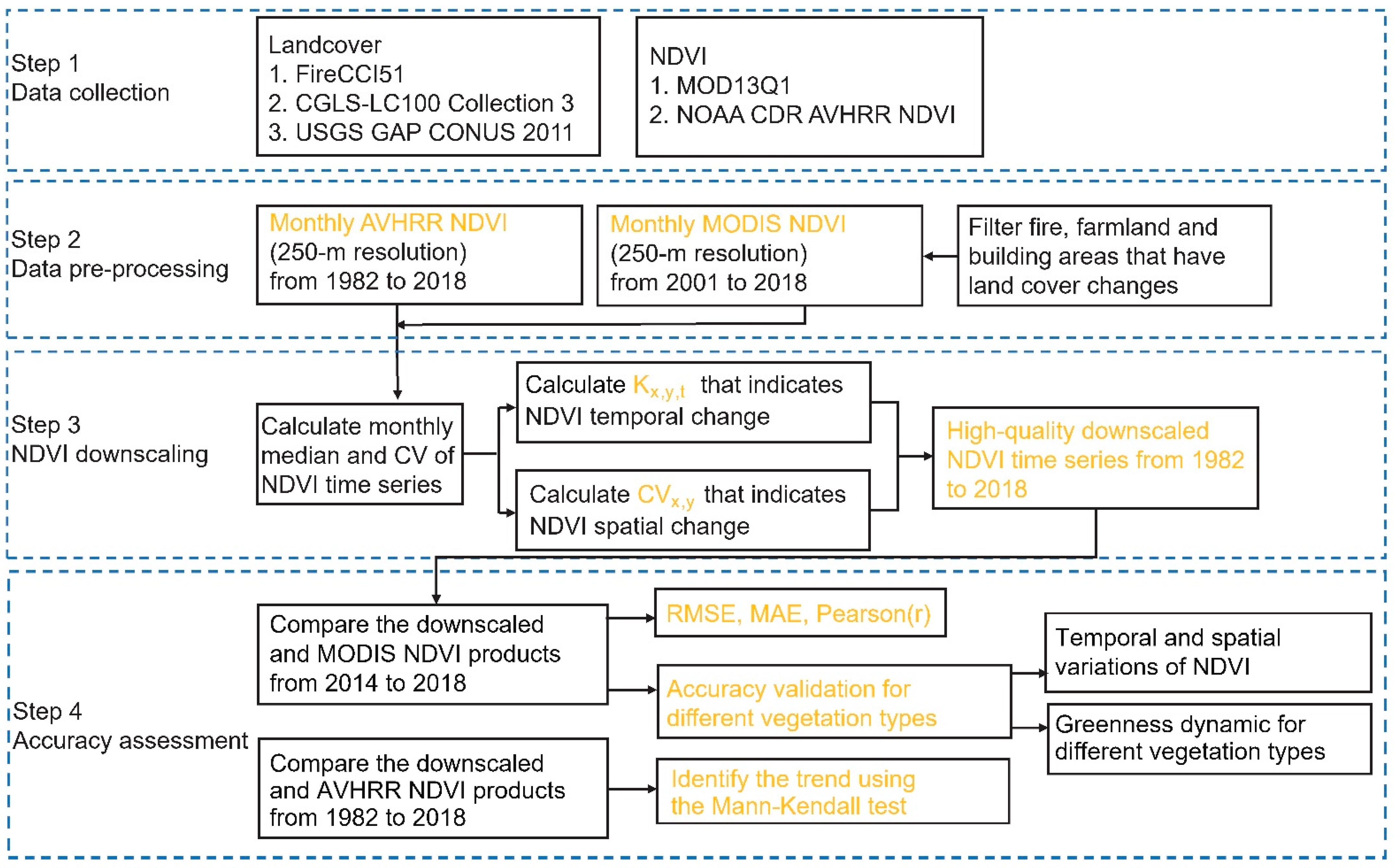
2.2.1. Data Pre-Processing (Steps 1–2)

We first integrated the daily AVHRR NDVI data and the 16-day MODIS NDVI data to the monthly time series. The MODIS and AVHRR NDVI results were composited into a monthly time series for each pixel using the Maximum Value Composite (MVC) approach, which extracted the pixelwise maximum NDVI value from all available NDVI observations within each month. The MVC approach takes the highest value for each pixel in a specific period (such as 10 days, a month, among other time spans) so that users can acquire a cloud-free, high-quality image [54]. We then resampled the AVHRR data to match the resolution of the MODIS NDVI using the bicubic spatial interpolation method. We removed the unnatural vegetation areas according to a land cover map.

2.2.2. Downscaling Algorithm (Step 3)

Since remote sensing data contain both temporal and spatial information, we downscaled the NDVI data at these two scales [55]. Previous studies suggest that, in an annual phenological cycle, combining the spatial characteristics of a single fine resolution image and the temporal characteristics (phenology) of a time series of coarse-resolution images can yield NDVI images with high spatial and temporal resolution [56,57]. In light of the above progress, herein we seek for the spatial change information in the fine-resolution MODIS NDVI and the temporal change information in the long-term AVHRR NDVI in the downscaling process.

(1)

Changes at the spatial scale

First, we quantified how these two NDVI products differed in pixelwise variability based on ratios of coefficient of variation (CV) between the MODIS and AVHRR NDVI. MODIS CV has a higher value than AVHRR CV in general because MODIS CV has more detailed spatial changing information. For example, while downscaling the coarse-resolution AVHRR data, the NDVI change degree should be increased for vegetation-dominated pixels that have many inter-annual changes in the NDVI. However, pixels with a high proportion of bare soil or buildings only exhibit minimal NDVI variations over time, resulting in compressed NDVI variability. Hence, we quantified the variability difference between MODIS and AVHRR products at each pixel using the $R_{CVx,y,m}$ ratio from 2001 to 2018 (Equation (1)).

$$R_{CVx,y,m}=MODIS\_CV/AVHRR\_C{V}_{post}$$

(1)

where $MODIS\_CV$ and $AVHRR\_C{V}_{post}$ are the pixelwise monthly coefficient of variation (CV) of the MODIS and AVHRR NDVI for the years 2001–2018, respectively.

However, the NDVI variability may demonstrate some changes over a long time period, for example from the 1980s to the 2000s. In downscaling the AVHRR product for the period prior to 2001, we used an additional parameter $R_{CVx,y,n}$ to quantify the relative changes in the AVHRR CV between the 1982–2000 and 2001–2018 periods (Equation (2)).

$$R_{CVx,y,n}=AVHRR\_C{V}_{pre}/AVHRR\_C{V}_{post}$$

(2)

where $AVHRR\_C{V}_{pre}$ and $AVHRR\_C{V}_{post}$ are the pixelwise monthly CV of the AVHRR NDVI for 1982–2000 and 2001–2018, respectively.

(2)

Changes at the temporal scale

We quantified the temporal changes in the NDVI by calculating the relative changes in each monthly NDVI against a baseline value using the coarse-resolution AVHRR product. The baseline value in the AVHRR NDVI product was computed as the per-pixel monthly NDVI median from 2001 to 2018, which was represented by $NDV{I}_{L,x,y,bl}$. Then, for each month of the time series, we compared each monthly AVHRR NDVI value to the baseline median of that month to determine the change degree. To define the temporal change, we employ the parameter $K_{x,y,t}$, which can capture the temporal information in the coarse-resolution AVHRR NDVI data at the time scale (Equation (3)).

$$K_{x,y,t}=\left(NDV{I}_{L,x,y,t}-NDV{I}_{L,x,y,bl}\right)/NDV{I}_{L,x,y,bl}$$

(3)

where $NDV{I}_{L,x,y,t}$ is the pixelwise monthly AVHRR NDVI in the entire time series (1982–2018), and $NDV{I}_{L,x,y,bl}$ is the baseline median NDVI in different months during the baseline period of 2001–2018. Please note that, for the period before 2000, the NDVI_L,x,y,bl was also computed as the per-pixel monthly NDVI median from 2001 to 2018, which helps keep the downscaled NDVI time series consistent over time.

(3)

Bringing together data on both spatial and temporal changes

The final phase of the downscaling combined the AVHRR product’s long-term temporal information with the MODIS product’s fine-scale spatial information (Equations (4) and (5)). The baseline value for MODIS was created using the per-pixel monthly NDVI median from 2001 to 2018 (shown by $NDV{I}_{H,x,y,bl}$ in the MODIS NDVI product). The corresponding monthly MODIS NDVI median was the fine-scale background NDVI at each pixel. Firstly, we divided the overall period into two parts, with the first period from 2001 to 2018. We multiplied the high-resolution baseline NDVI with the modifying parameters of $K_{x,y,t}$, and $R_{CVx,y,m}$, and then summed the results to indicate relative changes at both temporal and spatial scales, which was shown in Equation (4). Then, for the second period before 2000 without MODIS data, we multiplied an additional factor $R_{CVx,y,n}$ to describe the CV changes of AVHRR data between the two periods, as given in Equation (5). Finally, we can get the downscaled data using the formulas:

Period 2001–2018:

$$NDV{I}_{H,x,y,t}=NDV{I}_{H,x,y,bl}\times \left(1+K_{x,y,t}\times R_{CVx,y,m}\right)+{\epsilon }_{x,y,t }$$

(4)

Period 1982–2000:

$$NDV{I}_{H,x,y,t}=NDV{I}_{H,x,y,bl}\times \left(1+K_{x,y,t}\times R_{CVx,y,m}\times R_{CVx,y,n}\right)+{\epsilon }_{x,y,t }$$

(5)

where $NDV{I}_{H,x,y,t}$ is the downscaled high-resolution NDVI, $NDV{I}_{H,x,y,bl}$ is the monthly median MODIS NDVI (baseline NDVI), and ${\epsilon }_{x,y,t }$ is the random error generated in the downscaling process.

2.2.3. Error Validation (Step 4)

(1)

Evaluation Indices

We used three standard indices to validate the error between MODIS NDVI data and the downscaled NDVI data, and we used a timeframe of around 60 months from 2014 to 2018 to avoid data overfitting [58,59]. The evaluation indices are root mean square error (RMSE), mean absolute error (MAE), and Pearson’s correlation coefficient (Pearson’s R) and were calculated at the pixel level. RMSE is a commonly used measure of the difference between values and represents the sample standard deviation of the difference between the predicted and observed values. As a result, it offers a comprehensive evaluation of recalculation, including data retrieval accuracy and precision. We provided the RMSE map and calculated the mean for all pixels. MAE indicates the mean of the absolute error between the predicted and observed values and the value is determined directly for residuals. We calculated the MAE in each pixel and made the map. The Pearson’s correlation coefficient (Pearson’s R) is a frequently used metric for determining the degree of linear association between two variables. As a result, the accuracy at the spatial scale was estimated using Pearson’s correlation coefficient between the downscaled NDVI and MODIS NDVI at the pixel level.

(2)

Validation of accuracy for various vegetation types

To evaluate the overall applicability of the downscaling technique at the global scale, we chose eight typical vegetation patches of about 100 km² in size from the world vegetation map, and randomly selected one thousand pixels’ NDVI values in both the MODIS and the downscaled NDVI images for the validation period I to create linear fit lines. The vegetation types were derived from the Copernicus Landcover maps.

We assume high-resolution images can often provide more accurate spatial information, and we examined the capabilities of the three NDVI data sets to investigate NDVI variations in various vegetation types. We retrieved the median NDVI values for three types of vegetation in each month from all pixels in their respective ranges between July 2014 and June 2015, which indicated the average levels of greenness for each vegetation type. We then analyzed the NDVI time series to see if these three sources of data could accurately differentiate the three vegetation types.

(3)

Trend test of the downscaled NDVI time series

To validate the performance of the downscaled product in long-term vegetation monitoring, we used both the downscaled and AVHRR products to perform a Mann–Kendall test and a Sen’s slope estimation to compare the trends of the two datasets on the pixel scale [60,61]. Sen’s slope is a non-parametric statistical trend computation method that can lessen the incorrect influence of data outliers while accepting major data distributions [62]. We calculated a standard normal statistic (z) and divided it by its standard deviation to get the significance threshold. The z-P-value statistic (probability of detecting such an extreme value) is 1 − P (|z| Z). In general, the NDVI change trend has a significance of =0.05.

3. Results

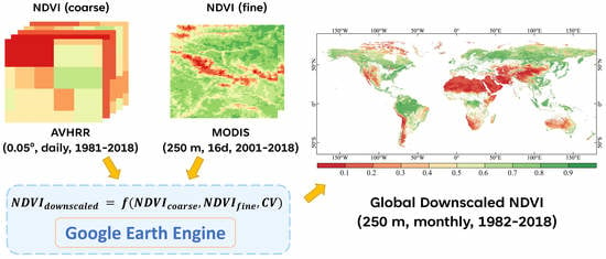
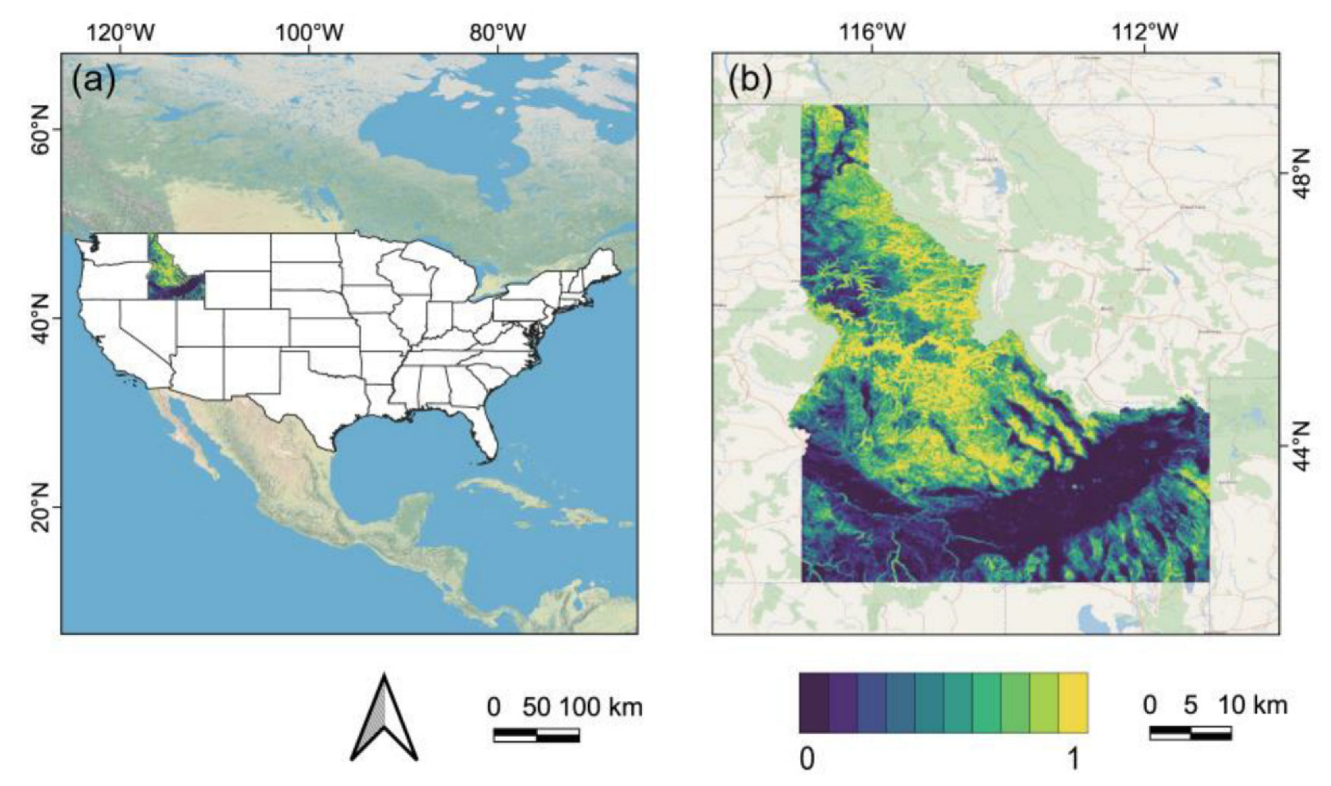
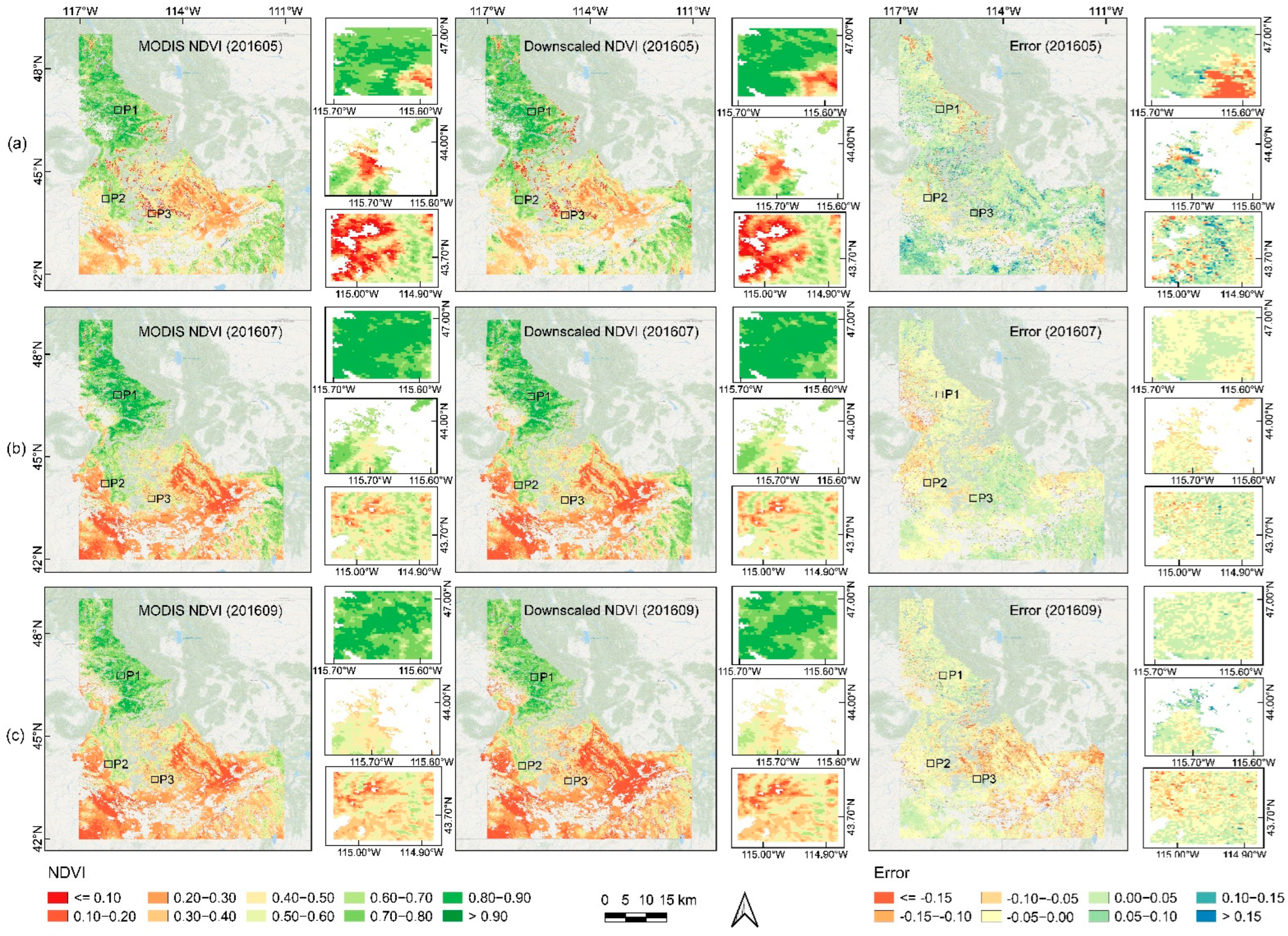
3.1. GEE Implementation in a Regional Area

To begin, we wanted to test the method in a regional setting, thus we chose Idaho state, in the northwest United States, as a case study location to demonstrate the NDVI downscaling technique due to its diversified geography and range of vegetation types. (Figure 2). We utilized the topographic diversity (D) as a metric to describe the range of temperature and moisture conditions that species can encounter in their local habitats (Figure 2b) [63]. The D value of most places approaches 1.0, indicating that Idaho has a wide range of topo-climate environments and a great diversity of plants. Idaho’s landscape can be divided into three regions: (1) the northern narrow strip and the mountainous parts, which are rich in timber; (2) the Snake River Plain, which runs through the state and is the state’s main agricultural sector; and (3) the southern mountainous region.

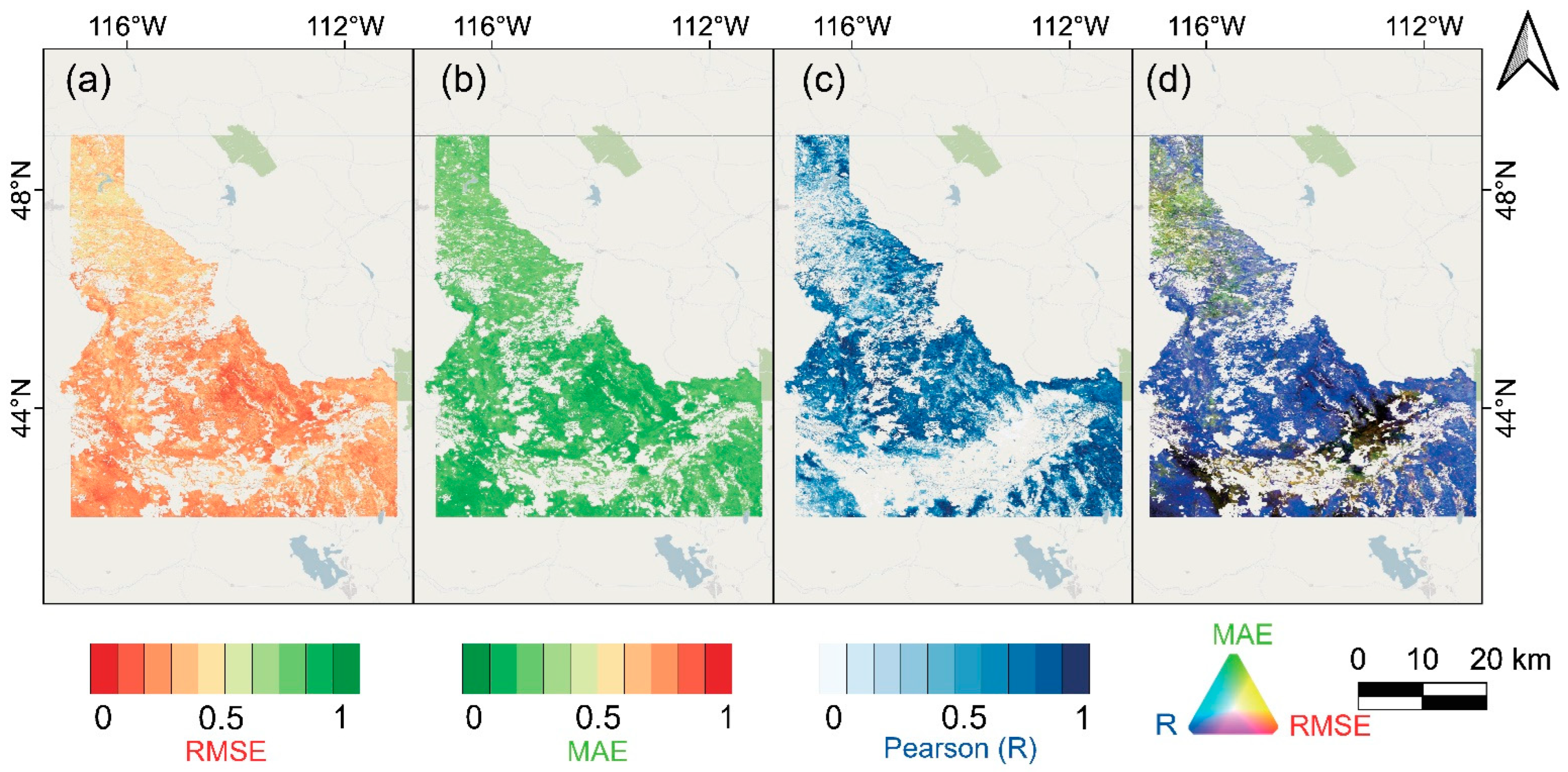
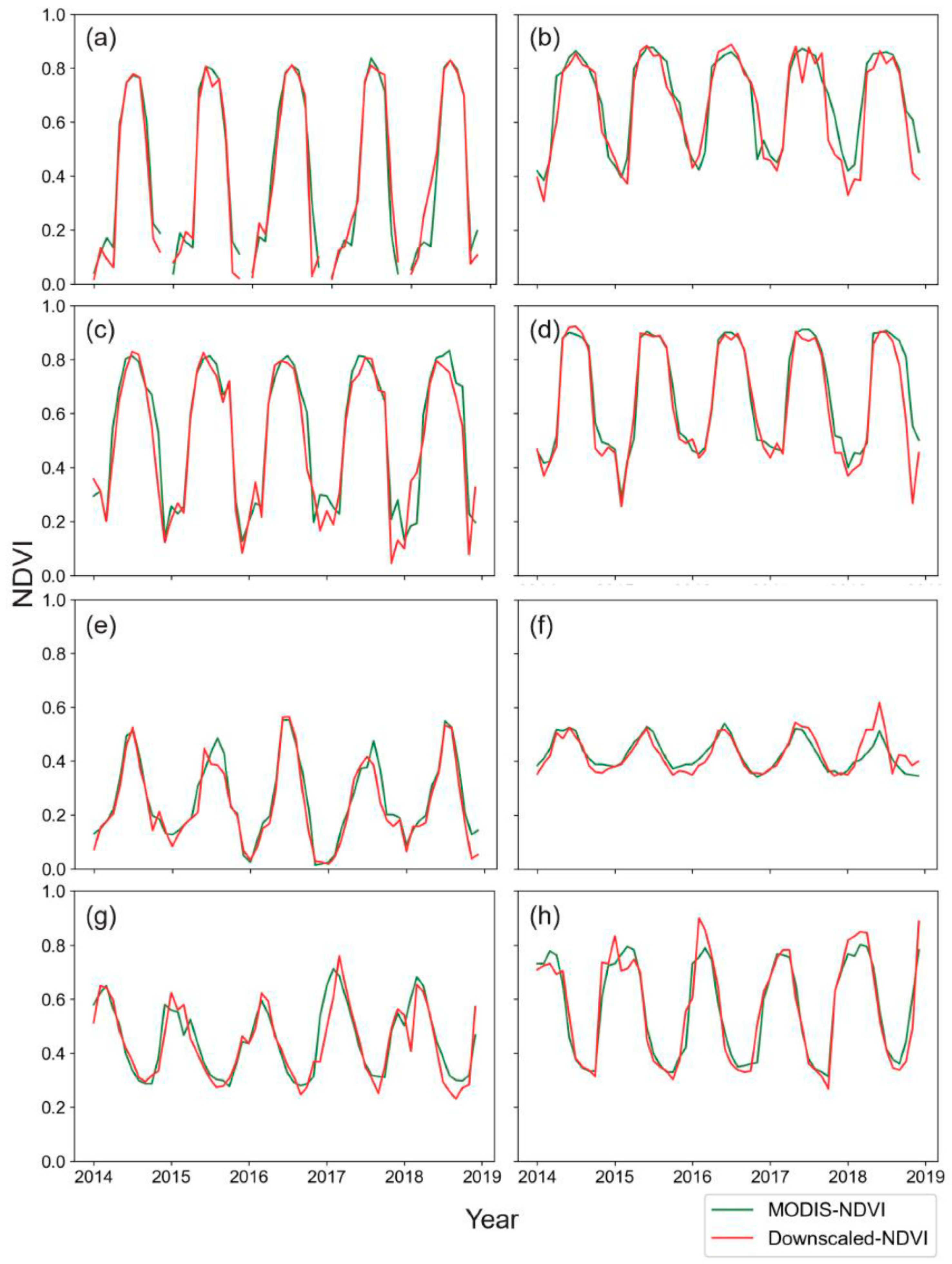
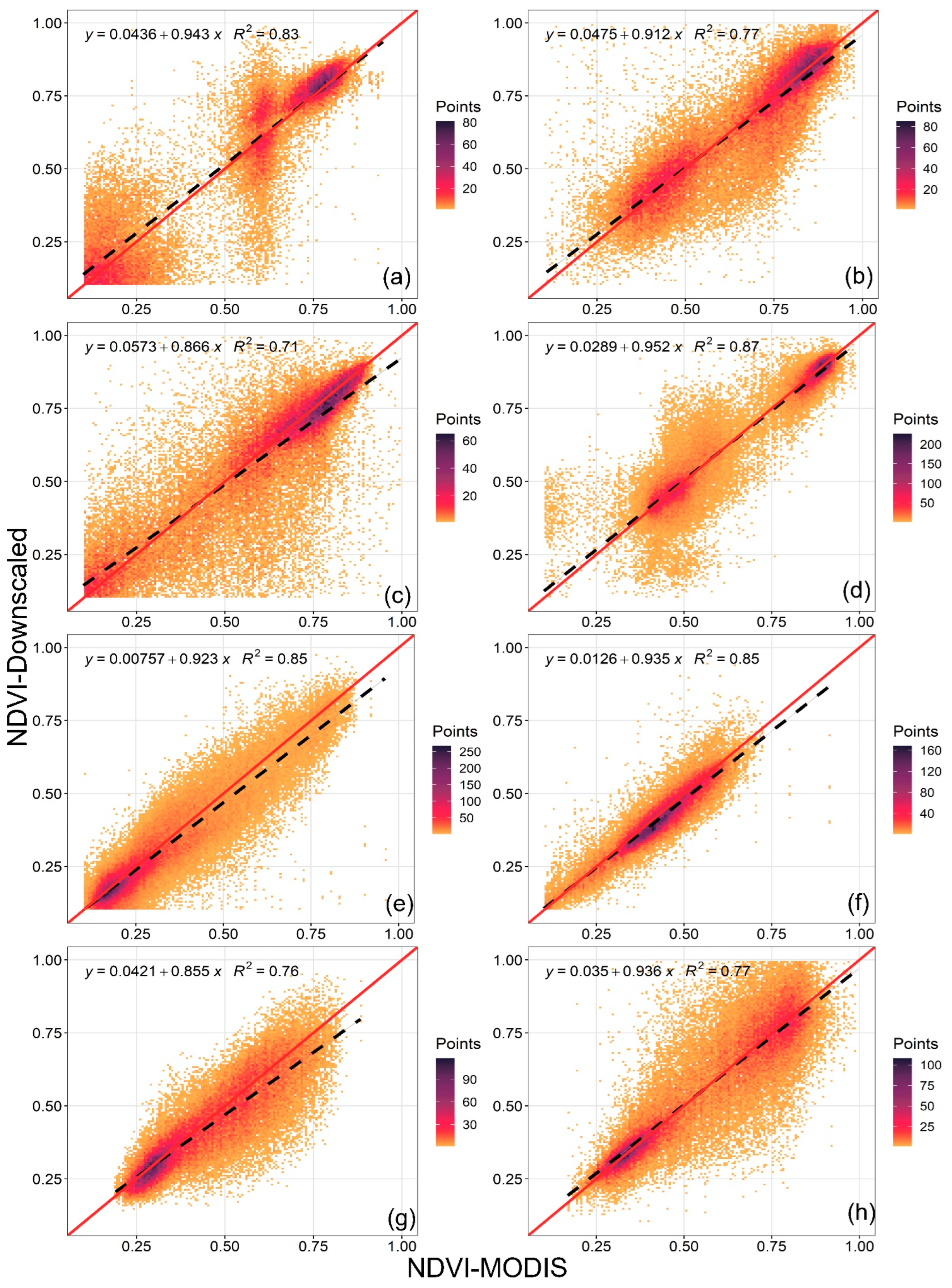
3.2. Validation at the Regional Scale

There were some examples of visual comparisons of the downscaled and standard MODIS NDVI, and we presented areas encompassing the entire state of Idaho as well as randomly selected smaller locations in Figure 3. Since the growing season offers more information about vegetation changes, we chose three downscaled NDVI images for the growing season (i.e., May, July, and September) in 2016 to compare to the MODIS NDVI product.

First, we carried out a comparison examination of the entire region, indicating the general difference between the two products was modest and the NDVI value distribution ranges were consistent with some subtle deviations in the spatial distribution of NDVI in some spots. Then, when we examined the dynamic changes in the vegetation growing season from May to September, we found that the greenness differences were noticeable from spring to autumn. The error of the majority of pixel values was between −0.05 and 0.05, as shown by mapping the differences between maps in Figure 3. The downscaled NDVI in the error map for May was higher than that of MODIS overall (more blue pixels), which was especially apparent in the southwest and central parts of Idaho. In contrast, the downscaled NDVI in July was not significantly different from the MODIS NDVI overall. Especially red pixels indicated a smaller downscaled NDVI in September compared to the overall MODIS NDVI, which was more pronounced in the eastern region.

Next, we chose three small portions (P1–P3 in Figure 3) around 30 km² in the vegetation-rich area to assess the accuracy of the downscaled outputs. Please note that the areas in patches 1 and 2 (P1, P2) were mainly dominated by evergreen needle leaves, and the area in patch 3 (P3) was mainly grass. Some slight discrepancies between the MODIS NDVI and the downscaled NDVI could be seen in these three small vegetation patches. The majority of the errors in the small area were often between −0.05 and 0.05, but the distinction was most noticeable in May, particularly to the southeast of P1. According to the NDVI distribution value, it is likely a transition zone between grassland and woodland. There is considerable inaccuracy here because different vegetation had varying green-up dates. Compared to the MODIS NDVI, the downscaled NDVI displayed some underestimation errors. Overall, the seasonal greenness dynamics between the two products were quite similar over time, with all of the inaccuracies being minor in the three vegetation patches (Figure 3).

The means of the three error indices in Idaho were then determined from the NDVI images shown in Figure 3, and the results are displayed below in

Table 1. Error statistics for the comparison between downscaled NDVI and MODIS NDVI of Idaho.

Time/Location	MAE	RMSE	Pearson’s R
201605 Idaho	0.047	0.069	0.926
201607 Idaho	0.033	0.052	0.974
201609 Idaho	0.052	0.076	0.961
201605-P1	0.062	0.097	0.871
201607-P1	0.015	0.020	0.930
201609-P1	0.016	0.023	0.939
201605-P2	0.061	0.077	0.925
201607-P2	0.035	0.045	0.946
201609-P2	0.034	0.046	0.822
201605-P3	0.053	0.071	0.950
201607-P3	0.030	0.041	0.946
201609-P3	0.034	0.048	0.927
Mean	0.039	0.055	0.926

. We obtained the mean value from all pixels in each location; in particular, for the calculation of Pearson’s R in Idaho, we randomly selected 1000 points approximately 1000 times to obtain the mean due to the large number of pixels in the entire state. The overall MAE, RMSE, and Pearson’s R are 0.039, 0.055, and 0.86, respectively, all showing an acceptable accuracy of the downscaled NDVI products. The biggest MAE and RMSE are less than 0.1, while the lowest Pearson’s R is greater than 0.8, indicating that the downscaling algorithm worked effectively for Idaho.

For each pixel of Idaho, we tested all three error indices of the downscaled NDVI dataset against the simultaneous MODIS NDVI, which reflected the errors produced by the downscaling procedure [64,65]. The validation maps of the RMSE, MAE, Pearson’s R, and RGB composite maps of these three indicators for all months from 2014 to 2018 are shown in Figure 4. The RMSEs and MAEs are low, mostly ranging between 0 to 0.2 (Figure 4a,b), and the correlating Pearson’s R values are high, ranging mostly from 0.7 to 1 (Figure 4c), implying that the downscaled NDVI errors are minor. The blue pixels in the RGB composite error map indicate that the downscaling technique is highly accurate (i.e., low RMSE, MAE, and high Pearson’s R), whereas the yellow pixels show areas with proportionally more errors (i.e., higher RMSE, MAE, and lower Pearson’s R), and the black pixels indicate that the values of the three indices are all small, indicating that the original data were lost. (Figure 5d) [65]. The majority of Idaho is displayed in blue, and a few black pixels refer to filtered crops. Additionally, yellow pixels are present mainly in the north, where the landscape is more undulating with a lot of forests, and these places therefore have relatively more uncertainty in the NDVI downscaling.

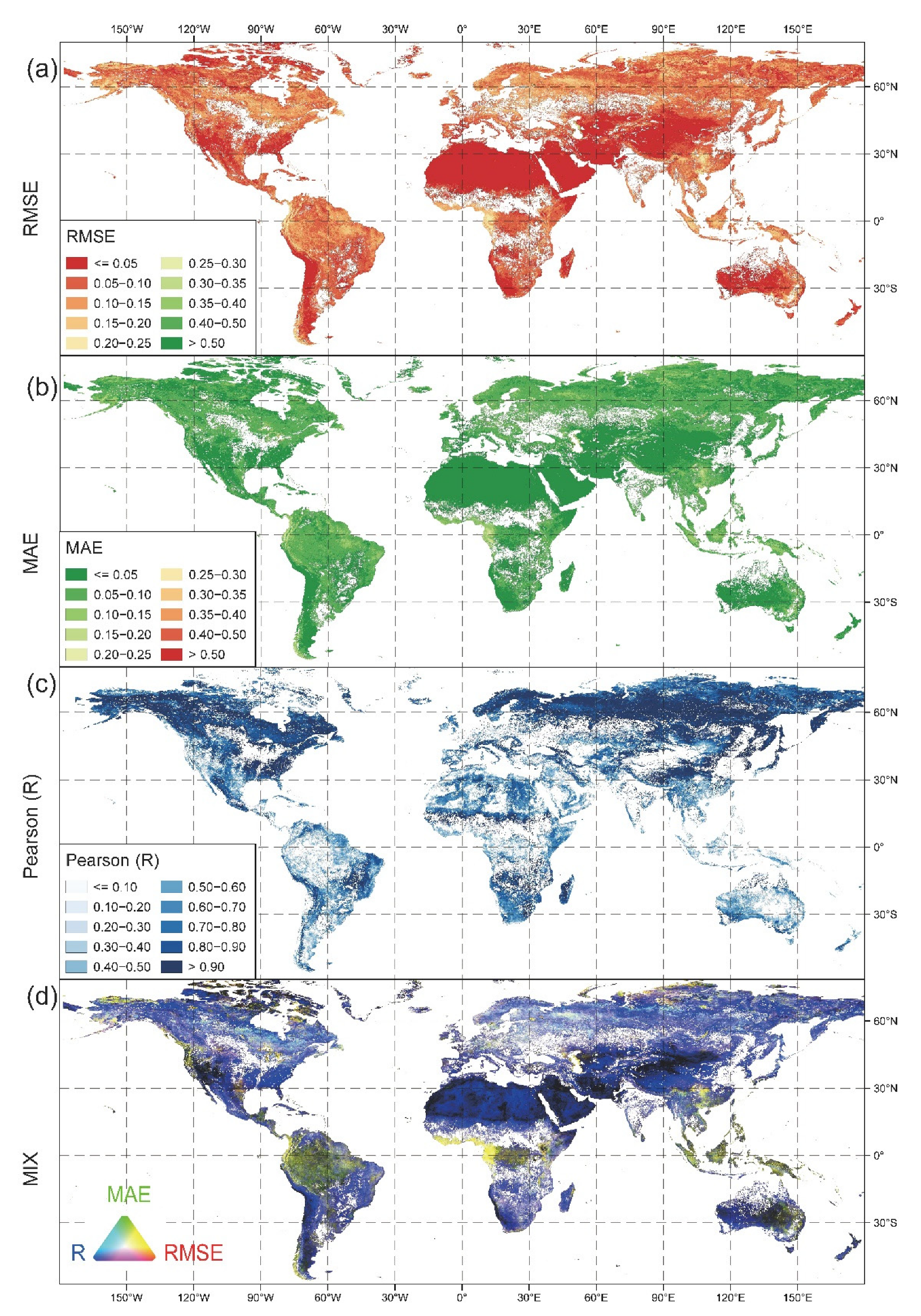
3.3. Validation at the Global Scale

In addition to the regional-scale study, we also performed the NDVI data downscaling on a global scale using GEE. We then further expanded the validation to the entire globe and evaluated the uncertainties of the data fusion algorithm for every pixel over the world for all months from 2014 to 2018 (Figure 5). Validation suggests that the majority of RMSE and MAE values fall between 0 and 0.1, according to the first observation (Figure 5a,b). The majority of Pearson’s R values are reasonably high and greater than 0.6, except for the tropics around the Equator, arid deserts, wastelands in Asia and Africa, and scant vegetation wilderness in Australia (Figure 5c).

The accuracy analysis was the same as for the Idaho error-index maps; however, the RGB map in Figure 5d, which combined the three error indices, provided more evident error information. As explained above, the different colors in the RGB composite error map reflect different levels of precision, so we focused on the black and yellow pixels.

First, we noticed that the black areas were typically found in sparsely vegetated areas, such as the central and eastern Asian desert regions and the Australian inland desert belts. Second, we saw that yellow pixels were concentrated in the tropics, indicating higher inaccuracy, which may be explained by the following two reasons. The first is related to a shift in land cover over the studied period; several studies have shown that many forests in Southeast Asia and South America are shrinking and being reclaimed as farmland since 2000, and frequent fires also cause forest loss, which implies that spatial changes are highly abrupt, and the sorts of ground objects change significantly [66,67]. The second reason is that the vegetation covers are dense in these areas, so the NDVI is easily saturated and cannot distinguish more seasonal changes in vegetation greenness. Indeed, the NDVI time series have been revealed to have strong data noise in the tropics, which could be caused by sub-pixel cloud contamination and a failure in the cloud filtering process [26,68]. Furthermore, some places of high altitudes and latitudes have larger RMSE and MAE and lower Pearson’s R (yellow in Figure 5d), likely owing to a high frequency of cloud and snow, which impedes satellite observations [65].

Overall, all three goodness of fit indicators (RMSE, MAE, and Pearson’s R) suggest that the downscaling algorithm performs well (blue in Figure 5d) in most parts of the world. As a result, using the proposed NDVI product for ecological applications at various scales should be safe. When running the code in areas with prolonged cloudiness and snow, as well as areas with dense rainforest or sparse vegetation, researchers should pay more attention to the uncertainties and errors of the approach, and strict validation is needed before applying the downscaled NDVI product.

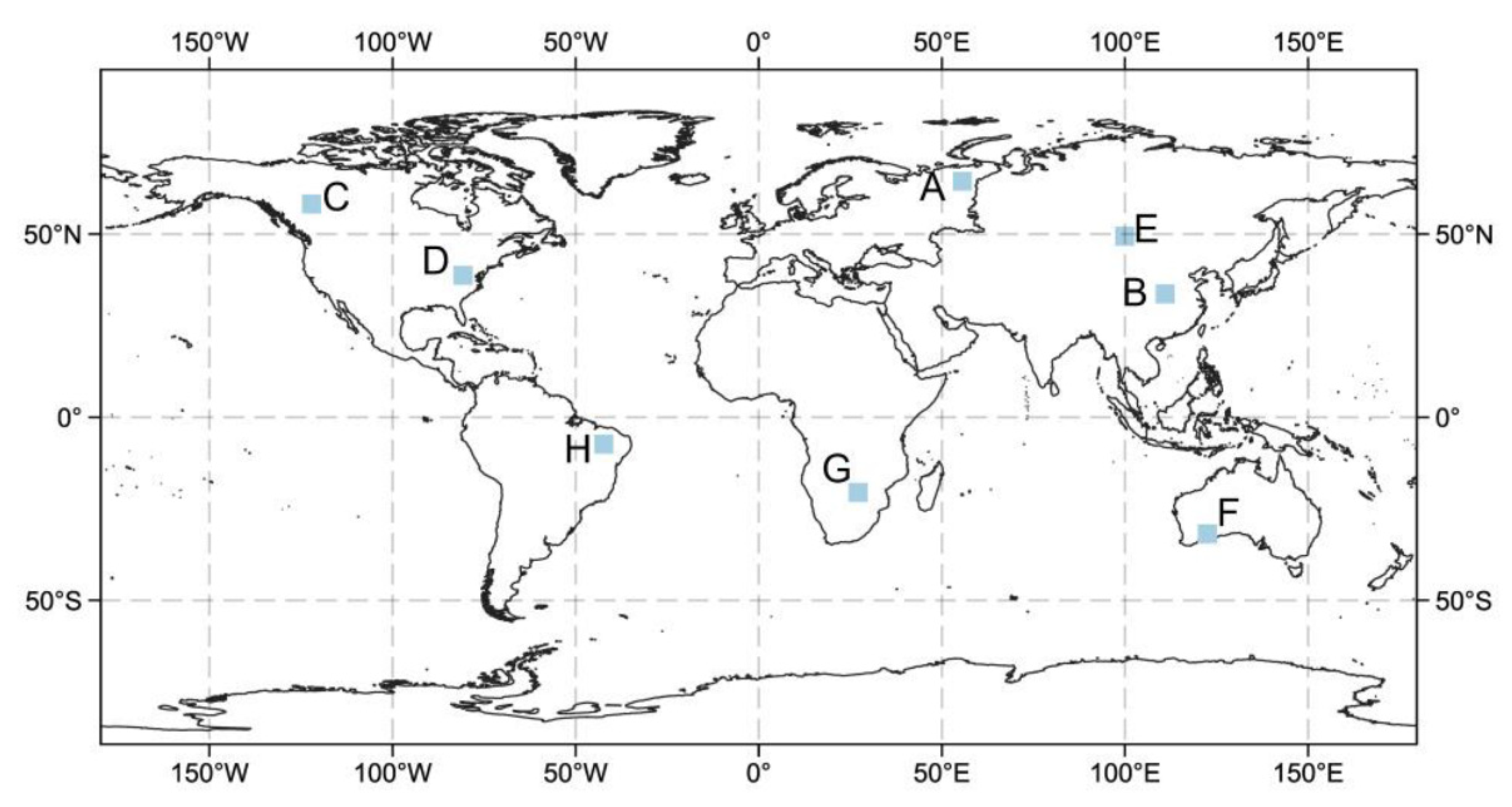
3.4. Validation for Different Vegetation Types

3.4.1. Comparison of Downscaled and MODIS NDVI Datasets for Global Major Vegetation Types

We used the Copernicus Global Land Cover dataset to obtain a global vegetation type map and then selected different representative vegetation types across continents to compare the MODIS NDVI and the downscaled NDVI. The validation was carried out at eight verification areas including many vegetation types with an area of approximately 100 km² around the world (Figure 6). The main vegetation types were coniferous forest, broad-leaved forest, grassland, and tropical shrub.

We investigated the accuracy of the downscaled NDVI applied to different vegetation types in two ways: (1) to demonstrate the capability of the downscaled data in synchronously capturing the seasonal greenness dynamics, we calculated and compared the monthly NDVI median time series derived from the two products from 2014 to 2018 (Figure 7); (2) to assess the overall performance of the downscaled data in accurately demonstrating the NDVI spatial changes, we randomly selected 1000 pixels’ NDVI values in both MODIS and the downscaled images for every month from 2014 to 2018 to make linear fit lines (Figure 8) [69].

Since terrestrial vegetation has such a large impact on the carbon cycle, energy exchange, and water balance of terrestrial ecosystems, studying the global and regional vegetation dynamics of NDVI on an annual and seasonal basis is critical [70,71]. Here, to make a temporal comparison, we chose the validation period from 2014 to 2018 and retrieved the monthly median as the basic level. Figure 7 depicted the eight types of vegetation changes through time, with the green lines representing the MODIS NDVI and the red lines representing the downscaled NDVI. We observed that the two lines were consistent overall. However, there were some noticeable biases between the two in 2015 and 2018 for some vegetation patches (e.g., the Australian Savanna and African Shrub, Figure 7f,g), indicating that there may be some disturbance factors affecting vegetation greenness, such as drought, fire, and so on [72].

Figure 8 depicts the linear fitting lines of the downscaled versus MODIS NDVI for the representative regions and vegetation types around the world. The fuchsia-point-concentrated areas highlighted where the majority of the NDVI values in each type of vegetation were in the plots, as well as how lush each vegetation community was. The most intensive range of grassland NDVI values, for example, was approximately 0 to 0.4 (Figure 8e,f), while the range of the forest was around the upper limit of the NDVI (0.8~1.0) (Figure 8a–d). To make this comparison, we randomly sampled 1000 pixels while considering both the geographical and temporal changes; hence, the results should be reliable. The downscaled NDVI data matched well with the MODIS NDVI, with reasonably high R² values (0.7~0.9). At the same time, the verifications suggest that the downscaled product can effectively capture the fine-scale NDVI dynamics and universal vegetation features.

As described above, the comparison and verification were carried out in time and space based on the NDVI seasonal time series and random sampling points across typical vegetation types over the globe. We might fairly infer that the downscaled NDVI product, which achieved both high resolution (250 m) and a long time frame (1982–2018), could be utilized as a good greenness indicator for monitoring much of the world’s vegetation communities.

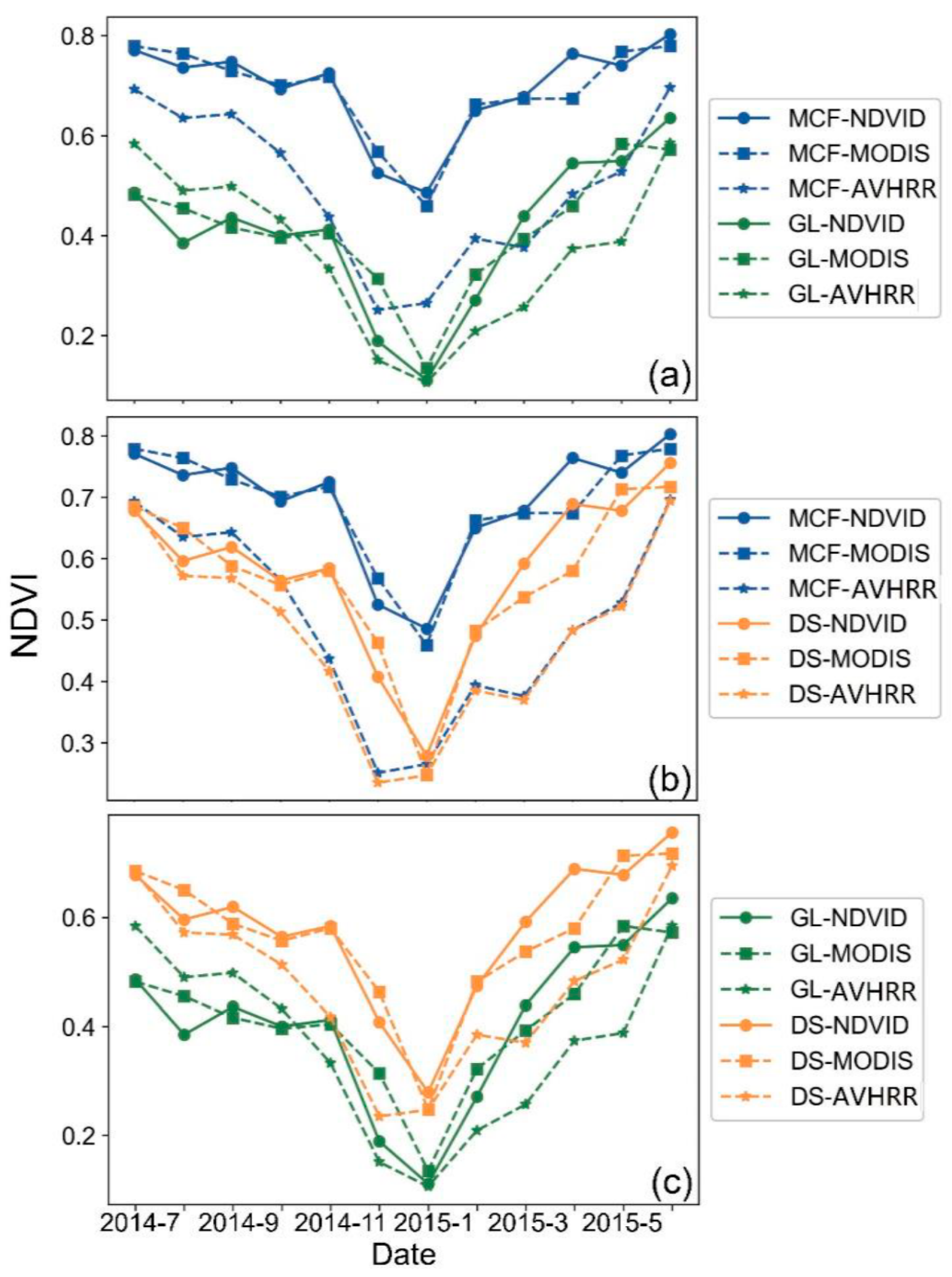
3.4.2. Comparison of the Three NDVI Datasets for Areas with Mixed Vegetation Types

We further compared the performance of the three NDVI datasets (MODIS, downscaled, and AVHRR) for areas with mixed vegetation types. This helped to determine the discriminating capability of the NDVI products. The GAP/LANDFIRE National Terrestrial Ecosystems database contains more detailed vegetation and land cover classifications, allowing us to delineate the extent of three major vegetation types in Idaho: the Northern Rocky Mountain Dry–Mesic Montane Mixed Conifer Forest (MCF), the Northern Rocky Mountain Lower Montane, Foothill and Valley Grassland (GL), and the Northern Rocky Mountain Montane–Foothill Deciduous Shrubland (DS) [73].

We found that the higher spatial resolution of the standard MODIS NDVI and the downscaled NDVI products both showed better performance than the AVHRR product in discriminating forest from other vegetation types, as suggested by the more visible curve differences between different vegetation types for the former two datasets (Figure 9a,b). As GL and DS have similar features, the differences were not generally apparent; however, MODIS and the downscaled NDVI still exhibit bigger differences than the AVHRR NDVI. In general, the downscaled and MODIS NDVI products with higher spatial resolution can both accurately recognize the greenness dynamics of different vegetation types, and their performance is similar. The AVHRR product displays poor performance when applied to mixed-vegetation areas, which might be caused by its lower spatial resolution and failure to characterize vegetation changes for heterogeneous regions.

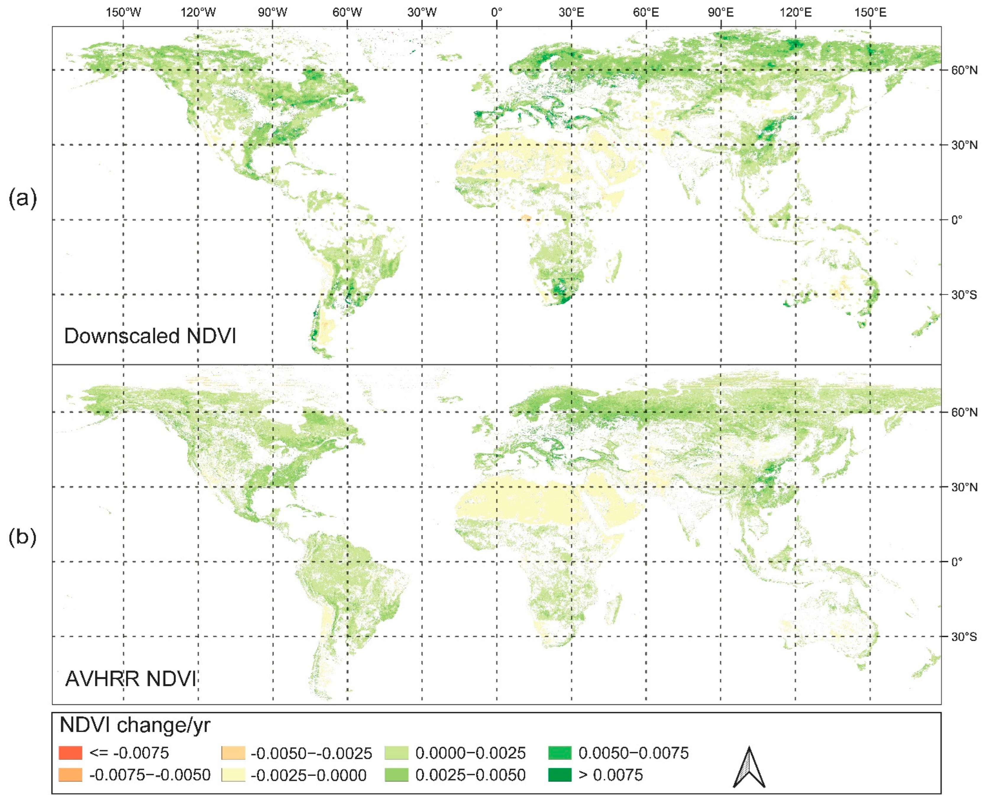
3.4.3. Comparison of the NDVI Change Trends from 1982 to 2018

We computed the median of the downscaled data, MODIS, and AVHRR NDVI across Idaho to illustrate regional averages. The period was separated into two parts, and the downscaled data were compared to the MODIS and AVHRR NDVI after 2000, as well as to the AVHRR NDVI before 2000. The findings are given as scatterplots in Figure S1, and the downscaled NDVI data for both periods fit well with MODIS and AVHRR products with high R² (about 0.9). To assess the capability of the downscaled NDVI products in depicting the large-scale greenness trends, we computed the interannual global NDVI trends using the MK trend test and Sen’s slope based on both the downscaled and AVHRR NDVI products (Figure 10). It can be seen that the results of the global NDVI trends derived from the two NDVI products are consistent with each other, reflecting the accuracy and reliability of the proposed product. At the same time, this spatial pattern is consistent with many previous studies: (1) the high latitude region and the Qinghai Tibet Plateau experienced a sustained increase in NDVI due to climate warming and the extension of the growing season [74,75]; (2) the NDVI was also increased due to afforestation in northern China and vegetation greening in the southern Sahara Desert [76,77].

4. Discussion

4.1. Value of the Downscaled NDVI Product

Satellite-based vegetation indices (VIs) have made a great contribution to the global to regional scale monitoring of terrestrial ecosystem dynamics. Many studies have revealed that over 25% to 50% of the global vegetated area displays a significant greening trend as a response to the rapid global environmental change, e.g., CO₂ fertilization, nitrogen deposition, climate change, and land cover change (LCC), etc. [75,78]. However, some recent studies suggest that the interannual variability of vegetation greenness has significantly increased over time [79], and widespread greening-to-browning reversals are hidden in the overall vegetation greening [80,81,82]. Nearly all of these important studies relied on the long-term but coarse-resolution AVHRR time series, or the fine-resolution but short-term MODIS product. The drawback in the vegetation database hinders the accurate estimation of plant activity under a changing climate. The inferior data might play a role in contradictory conclusions regarding the vegetation greenness trends in the literature.

In this paper, we proposed a novel data fusion approach that shows good performance in downscaling the coarse-resolution AVHRR NDVI (~5 km) to the MODIS resolution (250 m). The downscaled long-term (1982–2018) and high-resolution (250 m) global NDVI database has a high potential for accurately depicting the dynamics of trends, variability, and seasonality in the greenness of different vegetation communities at both global and regional scales, and it is particularly useful in mixed-vegetation areas. Compared to the previous downscaling approaches [36,37,38,39,40,41,44,45], the proposed algorithm is effective at reconciling simple computation and high accuracy.

4.2. Potential Causes of Discrepancies among Different Products

To test the accuracy of the downscaled NDVI product, we conducted rigorous validation of the product against the standard MODIS NDVI database at both the regional and global scales, and for different vegetation types. All the validation suggests a high accuracy of the downscaled NDVI product and the data fusion algorithm. The majority of RMSE and MAE values fall between 0 and 0.1 (Figure 5a,b), and the Pearson’s R values reach >0.7 for all the typical vegetation types over the globe (Figure 8). However, larger discrepancies between the two products are evident over the sparsely vegetated areas, and the equatorial belt (Figure 5d).

The large error in the sparsely vegetated areas is likely related to an inherent defect of the algorithm. Since the downscaling approach relies on analyzing the difference in the coefficient of variation (CV) between the AVHRR and MODIS NDVI databases, a slight change in the mean NDVI value for a sparsely vegetated area may lead to a big change in the CV. As a result, the algorithm will enlarge the difference between the two products and cause a large bias in the downscaled product.

The high deviations of the downscaled product in the equatorial belt should be related to the shortcomings of the NDVI itself, i.e., the NDVI easily reaches its saturated status in densely vegetated areas such as the tropical rainforest, which has been widely documented in the literature [26,68]. As a vegetation index, EVI (Enhanced Vegetation Index) is a good alternative to NDVI, and it appears to be superior in discriminating subtle differences in areas of high vegetation density, which can be attributed to the correction for atmospheric and background effects in the EVI algorithm [21]. However, the EVI time series is only available since entering the MODIS era, and its value is weakened by the short time span of the data, compared to NDVI database that has accumulated observations for several decades.

4.3. Uncertainties with the Downscaled NDVI Products

Mixed pixels make data downscaling challenging and induce uncertainties. Downscaling involves fusing two images with different resolutions, which results in some inaccuracies [83]. For example, in Figure 3, we can see that the discrepancy between the downscaling and MODIS NDVI is particularly noticeable in the P1 region, which is a heterogeneous region and has many mixed pixels.

Additionally, in the vegetation fusion field, our products may have errors at the micro spatial scale, but overall, these errors are acceptable, and the differences are small. Another issue is raised in the non-stationarity of NDVI time series, which exhibits various frequency components such as seasonal variations, long-term trends, and short-term variations [84]. The seasonal changes of the NDVI time series have been considered as the downscaling is executed on a monthly scale. However, when the coarse-resolution pixels are downscaled to fine-resolution pixels, if the pixels include mixed vegetation types, more deviations would be added. The time series of the NDVI in mixed pixels may exhibit increased instability due to the varying greening periods of plants.

Another uncertainty occurs as a result of the limited time period of the land cover maps. We removed the areas of unnatural vegetation before performing the downscaling computation using the land cover map and the fire map. There are no statistics on the fire areas before 2000 due to the map’s constrained coverage time, which only spans from 2000 to 2018. The land cover map ranges from 2015 to 2018, and there were no data for regions where crops and vegetation were interconverted prior to 2015. Forests in different locations may suffer from pests and diseases, experience significant drought, and produce short-term changes in vegetation. As a result, at the regional level, greater emphasis should be placed on the variety of land use types, as well as on the more rigorous verification of data quality and accuracy [85,86].

To assess the influence of topography on the performance of the downscaling algorithm, we compared the downscaled NDVI and MODIS NDVI along altitude during the growing season in 2016 in the Idaho area. We used the box diagrams to compare the NDVI quartiles of the two products for each elevation band from 800 to 2600 m at a 200-m interval. The results are displayed in Figure S2, which reveals that the difference between the two data was minimal along elevation gradients.

Some earlier studies have considered terrain changes in the downscaling of some environmental variables, e.g., land surface temperature [87,88]. Topography is also a highly important factor impacting NDVI distribution and has some potential in improving the algorithm accuracy. However, including topographic information in the downscaling on a worldwide scale is challenging since the global variation of the NDVI with topographical changes is extremely complicated [89]. The NDVI has a strong interaction with overall hydrothermal conditions, and there is no standard variation rule [90]. Among them, differences in slope, aspect, and vegetation band spectrum may have a significant influence on the NDVI. We can take into account the effect of terrain at the regional scale in the upcoming algorithm to increase the downscaling accuracy.

4.4. Limitations of the Downscaling Algorithm

The first constraint of the study is the low temporal resolution of the data, which is insufficient for phenological monitoring. The following issues exist when it comes to boosting temporal resolution. First, high-frequency changes in vegetation greenness are difficult to capture, and phenological oscillations differ amongst plant types. In this aspect, the algorithm in this study needs to be improved to include this information. Secondly, the NDVI is obviously disturbed by weather conditions in high-frequency data, and the data quality is poor [91,92]. In this paper’s approach, we restricted high-frequency data to increase the accuracy of lengthy time series. The primary benefit of the downscaling product described in this study is its spatial scale optimization, which can improve long-term dynamic monitoring of the fused vegetation area.

Another major limitation of the downscaling algorithm is that it is not suitable for areas that have experienced dramatic land use/cover changes (LUCCs), and thus we have removed the areas showing abrupt NDVI changes before the analyses. One important assumption of the proposed data fusion approach is that the vegetation type has not been replaced or removed during the studied period. This means that the variability of a vegetation community in greenness did not change much or maintained a relatively stable change. However, a long-term and gradual change in CV has been considered by the downscaling algorithm, as we have split the entire period into two portions (1982–2000 and 2001–2018), and an adjusting parameter ($R_{CVx,y,n}$) has been used to quantify the long-term changes in CV of vegetation greenness (Equation (2)). Hence, the downscaled NDVI product should be useful in capturing both the short-term dynamics and long-term trends in vegetation greenness, which reflects vegetation flourishing, deterioration, and restoration due to climate change, drought, competition, etc. However, LUCC has become an important phenomenon of global environmental change and it can directly modify the type, structure, and function of an ecological system, resulting in changes in the vegetation of that system [93,94]. Thus, it is of high significance to develop more robust data fusion techniques for satellite-based vegetation indices, which is feasible for the areas experiencing dramatic LUCCs.

In addition, we did not extend the time span of the downscaled NDVI product beyond 2018, since the AVHRR sensor has degraded since late 2018, and the NOAA AVHRR NDVI database displays widespread data gaps in the southern hemisphere after 2018 [62]. However, the major purpose of this study is to extend the MODIS resolution NDVI database to the pre-2000 period. A 38-year, high-resolution NDVI time series should have many more advantages than the 22-year MODIS NDVI product in analyzing the long-term trends of global vegetation dynamics.

4.5. Future Improvements

In the subsequent work, the following aspects can be improved. Firstly, we suggest integrating high temporal–resolution products, creating methods to capture high-frequency information, and combining wavelet and Fourier transforms to increase the temporal resolution of the downscaled product [91,95]. The next step is to merge higher spatial–resolution NDVI data, such as the Landsat satellite data, with higher-precision land cover maps and terrain data (data elevation models) in order to expand the product’s accuracy in both mixed vegetation regions and areas with complicated topography.

Secondly, the approach may be integrated with other methods such as machine learning, geostatistical simulation methods, and fractal and multifractal methods. As mentioned above, remote sensing data typically contains many data gaps due to clouds, cloud shadows, and even systemic inaccuracies, and therefore the quality of high-frequency temporal data is generally bad [96]. Direct sampling (DS) methods are analog approaches that can be used to fill gaps in remote sensing data and improve image temporal resolution [97,98]. Mariethoz et al. [99] attempted to locate a known pixel whose neighbors have similar values that are comparable to the unknown pixel’s neighbors, and then filled in the pixel’s value with the known value. In this case, we may combine DS with machine learning algorithms to fill in temporal gaps and enhance data frequency. Among the widely used scale transformation methodologies, fractal theory accurately depicts how the study item changes when the scale is changed [35,100]. The fractal technique uses fewer parameters to offer a more basic and explicit explanation of object spatiotemporal changes, resulting in a more realistic scale transformation model [101]. Several fractal and multifractal algorithms were used to downscale satellite-based remote sensing rainfall data and scale the leaf area index [102,103]. At the same time, this approach may be utilized for NDVI downscaling.

5. Conclusions

GEE is used as the operation platform in this work to undertake a long-term and global-scale data fusion of remotely sensed vegetation index data. The primary idea behind our technique was to extract the fine-scale NDVI spatial information from the high-resolution MODIS images and then integrate it with the long-term NDVI temporal information from the AVHRR database. Finally, we created a downscaled 250-m resolution global NDVI dataset from 1982 to 2018, and the data quality was compared to the standard MODIS NDVI products at both the regional and global scales. The RMSE and MAE are less than 0.1 in most locations, and the Pearson’s R is typically greater than 0.6, according to the validation results. However, in locations demonstrating abrupt landcover changes, the downscaled product may contain bigger biases and may therefore require further improvement in the future. Additionally, the low temporal resolution of the downscaled NDVI product weakens its value in phenological studies, which should be fixed in future studies. The good performance of the downscaling algorithm likely suggests that the coefficient of variation (CV) could be a valuable intermediary for combining the fine- and coarse-resolution remote sensing data. The downscaled global NDVI product demonstrates great potential for investigating the global plant response to climate change, and for monitoring the fine-scale (250 m) and long-term (four decades) vegetation dynamics in facing different types of environmental stress.

References

1. Rustad, L.E. The response of terrestrial ecosystems to global climate change: Towards an integrated approach. Sci. Total Environ. 2008, 404, 222–235. [Google Scholar] [CrossRef] [PubMed]
2. Myneni, R.B.; Keeling, C.D.; Tucker, C.J.; Asrar, G.; Nemani, R.R. Increased plant growth in the northern high latitudes from 1981 to 1991. Nature 1997, 386, 698–702. [Google Scholar] [CrossRef]
3. Zeebe, R.E.; Ridgwell, A.; Zachos, J.C. Anthropogenic carbon release rate unprecedented during the past 66 million years. Nat. Geosci. 2016, 9, 325–329. [Google Scholar] [CrossRef] [Green Version]
4. Lenssen, N.J.L.; Schmidt, G.A.; Hansen, J.E.; Menne, M.J.; Persin, A.; Ruedy, R.; Zyss, D. Improvements in the GISTEMP Uncertainty Model. J. Geophys. Res. Atmos. 2019, 124, 6307–6326. [Google Scholar] [CrossRef]
5. Lamprecht, A.; Semenchuk, P.R.; Steinbauer, K.; Winkler, M.; Pauli, H. Climate change leads to accelerated transformation of high-elevation vegetation in the central Alps. New Phytol. 2018, 220, 447–459. [Google Scholar] [CrossRef]
6. Field, C.B.; Barros, V.R. Climate Change 2014–Impacts, Adaptation and Vulnerability: Regional Aspects; Cambridge University Press: Cambridge, UK, 2014. [Google Scholar]
7. Diffenbaugh, N.S.; Singh, D.; Mankin, J.S.; Horton, D.E.; Swain, D.L.; Touma, D.; Charland, A.; Liu, Y.; Haugen, M.; Tsiang, M.; et al. Quantifying the influence of global warming on unprecedented extreme climate events. Proc. Natl. Acad. Sci. USA 2017, 114, 4881–4886. [Google Scholar] [CrossRef] [PubMed] [Green Version]
8. Papalexiou, S.M.; Montanari, A. Global and Regional Increase of Precipitation Extremes Under Global Warming. Water Resour. Res. 2019, 55, 4901–4914. [Google Scholar] [CrossRef]
9. Warren, R.; Price, J.; Fischlin, A.; de la Santos, S.N.; Midgley, G. Increasing impacts of climate change upon ecosystems with increasing global mean temperature rise. Clim. Chang. 2011, 106, 141–177. [Google Scholar] [CrossRef]
10. Hoegh-Guldberg, O.; Jacob, D.; Bindi, M.; Brown, S.; Camilloni, I.; Diedhiou, A.; Djalante, R.; Ebi, K.; Engelbrecht, F.; Guiot, J.; et al. Impacts of 1.5 °C global warming on natural and human systems. In Global Warming of 1.5 °C; World Meteorological Organization: Geneva, Switzerland, 2018. [Google Scholar]
11. Li, D.; Wu, S.; Liu, L.; Zhang, Y.; Li, S. Vulnerability of the global terrestrial ecosystems to climate change. Glob. Chang. Biol. 2018, 24, 4095–4106. [Google Scholar] [CrossRef]
12. Peters, A.J.; Walter-Shea, E.A.; Ji, L.; Vina, A.; Hayes, M.; Svoboda, M.D. Drought monitoring with NDVI-based Standardized Vegetation Index. Photogramm. Eng. Remote Sens. 2002, 68, 71–75. [Google Scholar]
13. Gu, Y.; Wylie, B.K. Downscaling 250-m MODIS Growing Season NDVI Based on Multiple-Date Landsat Images and Data Mining Approaches. Remote Sens. 2015, 7, 3489–3506. [Google Scholar] [CrossRef] [Green Version]
14. Huete, A.; Didan, K.; Miura, T.; Rodriguez, E.P.; Gao, X.; Ferreira, L.G. Overview of the radiometric and biophysical performance of the MODIS vegetation indices. Remote Sens. Environ. 2002, 83, 195–213. [Google Scholar] [CrossRef]
15. Tucker, C.J. Red and photographic infrared linear combinations for monitoring vegetation. Remote Sens. Environ. 1979, 8, 127–150. [Google Scholar] [CrossRef] [Green Version]
16. Brown, M.E.; Lary, D.J.; Vrieling, A.; Stathakis, D.; Mussa, H. Neural networks as a tool for constructing continuous NDVI time series from AVHRR and MODIS. Int. J. Remote Sens. 2008, 29, 7141–7158. [Google Scholar] [CrossRef] [Green Version]
17. Tarnavsky, E.; Garrigues, S.; Brown, M.E. Multiscale geostatistical analysis of AVHRR, SPOT-VGT, and MODIS global NDVI products. Remote Sens. Environ. 2008, 112, 535–549. [Google Scholar] [CrossRef]
18. Stellmes, M.; Udelhoven, T.; Röder, A.; Sonnenschein, R.; Hill, J. Dryland observation at local and regional scale—Comparison of Landsat TM/ETM+ and NOAA AVHRR time series. Remote Sens. Environ. 2010, 114, 2111–2125. [Google Scholar] [CrossRef]
19. Sano, E.E.; Ferreira, L.G.; Asner, G.; Steinke, E.T. Spatial and temporal probabilities of obtaining cloud-free Landsat images over the Brazilian tropical savanna. Int. J. Remote Sens. 2007, 28, 2739–2752. [Google Scholar] [CrossRef]
20. Anderson, M.C.; Yang, Y.; Xue, J.; Knipper, K.R.; Yang, Y.; Gao, F.; Hain, C.R.; Kustas, W.P.; Cawse-Nicholson, K.; Hulley, G.; et al. Interoperability of ECOSTRESS and Landsat for mapping evapotranspiration time series at sub-field scales. Remote Sens. Environ. 2021, 252, 112189. [Google Scholar] [CrossRef]
21. Didan, K.; Munoz, A.B.; Solano, R.; Huete, A. MODIS Vegetation Index User’s Guide (MOD13 Series); University of Arizona, Vegetation Index and Phenology Lab: Tucson, AZ, USA, 2015. [Google Scholar]
22. van Leeuwen, W.J.D.; Orr, B.J.; Marsh, S.E.; Herrmann, S.M. Multi-sensor NDVI data continuity: Uncertainties and implications for vegetation monitoring applications. Remote Sens. Environ. 2006, 100, 67–81. [Google Scholar] [CrossRef]
23. Rao, Y.; Zhu, X.; Chen, J.; Wang, J. An Improved Method for Producing High Spatial-Resolution NDVI Time Series Datasets with Multi-Temporal MODIS NDVI Data and Landsat TM/ETM+ Images. Remote Sens. 2015, 7, 7865–7891. [Google Scholar] [CrossRef] [Green Version]
24. Lunetta, R.S.; Knight, J.F.; Ediriwickrema, J.; Lyon, J.G.; Worthy, L.D. Land-cover change detection using multi-temporal MODIS NDVI data. Remote Sens. Environ. 2006, 105, 142–154. [Google Scholar] [CrossRef]
25. Wang, X.; Li, Y.; Wang, X.; Li, Y.; Lian, J.; Gong, X. Temporal and Spatial Variations in NDVI and Analysis of the Driving Factors in the Desertified Areas of Northern China From 1998 to 2015. Front. Environ. Sci. 2021, 9, 633020. [Google Scholar] [CrossRef]
26. Zhu, X.; Liu, D. Improving forest aboveground biomass estimation using seasonal Landsat NDVI time-series. ISPRS J. Photogramm. Remote Sens. 2015, 102, 222–231. [Google Scholar] [CrossRef]
27. Zeng, L.; Wardlow, B.D.; Xiang, D.; Hu, S.; Li, D. A review of vegetation phenological metrics extraction using time-series, multispectral satellite data. Remote Sens. Environ. 2020, 237, 111511. [Google Scholar] [CrossRef]
28. Pradhan, N.R.; Tachikawa, Y.; Takara, K. A downscaling method of topographic index distribution for matching the scales of model application and parameter identification. Hydrol. Process. 2006, 20, 1385–1405. [Google Scholar] [CrossRef]
29. Wang, Q.; Shi, W.; Atkinson, P.M.; Zhao, Y. Downscaling MODIS images with area-to-point regression kriging. Remote Sens. Environ. 2015, 166, 191–204. [Google Scholar] [CrossRef]
30. Chen, Y.; Huang, J.; Sheng, S.; Mansaray, L.R.; Liu, Z.; Wu, H.; Wang, X. A new downscaling-integration framework for high-resolution monthly precipitation estimates: Combining rain gauge observations, satellite-derived precipitation data and geographical ancillary data. Remote Sens. Environ. 2018, 214, 154–172. [Google Scholar] [CrossRef]
31. Piles, M.; Camps, A.; Vall-llossera, M.; Corbella, I.; Panciera, R.; Rudiger, C.; Kerr, Y.H.; Walker, J. Downscaling SMOS-Derived Soil Moisture Using MODIS Visible/Infrared Data. IEEE Trans. Geosci. Remote Sens. 2011, 49, 3156–3166. [Google Scholar] [CrossRef]
32. Kou, X.; Jiang, L.; Bo, Y.; Yan, S.; Chai, L. Estimation of Land Surface Temperature through Blending MODIS and AMSR-E Data with the Bayesian Maximum Entropy Method. Remote Sens. 2016, 8, 105. [Google Scholar] [CrossRef] [Green Version]
33. Qu, Y.; Zhu, Z.; Montzka, C.; Chai, L.; Liu, S.; Ge, Y.; Liu, J.; Lu, Z.; He, X.; Zheng, J.; et al. Inter-comparison of several soil moisture downscaling methods over the Qinghai-Tibet Plateau, China. J. Hydrol. 2021, 592, 125616. [Google Scholar] [CrossRef]
34. Gruber, A.; De Lannoy, G.; Albergel, C.; Al-Yaari, A.; Brocca, L.; Calvet, J.C.; Colliander, A.; Cosh, M.; Crow, W.; Dorigo, W.; et al. Validation practices for satellite soil moisture retrievals: What are (the) errors? Remote Sens. Environ. 2020, 244, 111806. [Google Scholar] [CrossRef]
35. Ge, Y.; Jin, Y.; Stein, A.; Chen, Y.; Wang, J.; Wang, J.; Cheng, Q.; Bai, H.; Liu, M.; Atkinson, P.M. Principles and methods of scaling geospatial Earth science data. Earth-Sci. Rev. 2019, 197, 102897. [Google Scholar] [CrossRef]
36. Settle, J.J.; Drake, N.A. Linear mixing and the estimation of ground cover proportions. Int. J. Remote Sens. 1993, 14, 1159–1177. [Google Scholar] [CrossRef]
37. Kerdiles, H.; Grondona, M.O. NOAA-AVHRR NDVI decomposition and subpixel classification using linear mixing in the Argentinean Pampa. Int. J. Remote Sens. 1995, 16, 1303–1325. [Google Scholar] [CrossRef]
38. Somers, B.; Asner, G.P.; Tits, L.; Coppin, P. Endmember variability in Spectral Mixture Analysis: A review. Remote Sens. Environ. 2011, 115, 1603–1616. [Google Scholar] [CrossRef]
39. Feng, G.; Masek, J.; Schwaller, M.; Hall, F. On the blending of the Landsat and MODIS surface reflectance: Predicting daily Landsat surface reflectance. IEEE Trans. Geosci. Remote Sens. 2006, 44, 2207–2218. [Google Scholar] [CrossRef]
40. Hilker, T.; Wulder, M.; Coops, N.; Linke, J.; McDermid, G.; Masek, J.G.; Gao, F.; White, J. A new data fusion model for high spatial- and temporal-resolution mapping of forest disturbance based on Landsat and MODIS. Remote Sens. Environ. 2009, 113, 1613–1627. [Google Scholar] [CrossRef]
41. Zhu, X.; Chen, J.; Gao, F.; Chen, X.; Masek, J.G. An enhanced spatial and temporal adaptive reflectance fusion model for complex heterogeneous regions. Remote Sens. Environ. 2010, 114, 2610–2623. [Google Scholar] [CrossRef]
42. Cui, J.; Zhang, X.; Luo, M. Combining Linear Pixel Unmixing and STARFM for Spatiotemporal Fusion of Gaofen-1 Wide Field of View Imagery and MODIS Imagery. Remote Sens. 2018, 10, 1047. [Google Scholar] [CrossRef] [Green Version]
43. Xue, J.; Leung, Y.; Fung, T. An Unmixing-Based Bayesian Model for Spatio-Temporal Satellite Image Fusion in Heterogeneous Landscapes. Remote Sens. 2019, 11, 324. [Google Scholar] [CrossRef] [Green Version]
44. Htitiou, A.; Boudhar, A.; Benabdelouahab, T. Deep Learning-Based Spatiotemporal Fusion Approach for Producing High-Resolution NDVI Time-Series Datasets. Can. J. Remote Sens. 2021, 47, 182–197. [Google Scholar] [CrossRef]
45. Nomura, R.; Oki, K. Downscaling of MODIS NDVI by Using a Convolutional Neural Network-Based Model with Higher Resolution SAR Data. Remote Sens. 2021, 13, 732. [Google Scholar] [CrossRef]
46. Buhrmester, V.; Münch, D.; Arens, M. Analysis of Explainers of Black Box Deep Neural Networks for Computer Vision: A Survey. Mach. Learn. Knowl. Extr. 2021, 3, 966–989. [Google Scholar] [CrossRef]
47. Colin Koeniguer, E.; Nicolas, J.-M. Change Detection Based on the Coefficient of Variation in SAR Time-Series of Urban Areas. Remote Sens. 2020, 12, 2089. [Google Scholar] [CrossRef]
48. Wang, R.; Gamon, J.A.; Emmerton, C.A.; Li, H.; Nestola, E.; Pastorello, G.Z.; Menzer, O. Integrated Analysis of Productivity and Biodiversity in a Southern Alberta Prairie. Remote Sens. 2016, 8, 214. [Google Scholar] [CrossRef] [Green Version]
49. Gorelick, N.; Hancher, M.; Dixon, M.; Ilyushchenko, S.; Thau, D.; Moore, R. Google Earth Engine: Planetary-scale geospatial analysis for everyone. Remote Sens. Environ. 2017, 202, 18–27. [Google Scholar] [CrossRef]
50. Tian, F.; Wu, B.; Zeng, H.; Zhang, X.; Xu, J. Efficient Identification of Corn Cultivation Area with Multitemporal Synthetic Aperture Radar and Optical Images in the Google Earth Engine Cloud Platform. Remote Sens. 2019, 11, 629. [Google Scholar] [CrossRef] [Green Version]
51. Zhai, H.; Zhang, H.; Zhang, L.; Li, P. Cloud/shadow detection based on spectral indices for multi/hyperspectral optical remote sensing imagery. ISPRS J. Photogramm. Remote Sens. 2018, 144, 235–253. [Google Scholar] [CrossRef]
52. Chen, Y.; Sun, K.; Chen, C.; Bai, T.; Park, T.; Wang, W.; Nemani, R.R.; Myneni, R.B. Generation and Evaluation of LAI and FPAR Products from Himawari-8 Advanced Himawari Imager (AHI) Data. Remote Sens. 2019, 11, 1517. [Google Scholar] [CrossRef] [Green Version]
53. Vermote, E.; Justice, C.; Csiszar, I.; Eidenshink, J.; Myneni, R.; Baret, F.; Masuoka, E.; Wolfe, R.; Claverie, M. NOAA Climate Data Record (CDR) of Normalized Difference Vegetation Index (NDVI), Version 4; NOAA’s National Climatic Data Center: Asheville, NC, USA, 2014. [Google Scholar] [CrossRef]
54. Faisal, B.M.R.; Rahman, H.; Sharifee, N.H.; Sultana, N.; Islam, M.I.; Ahammad, T. Remotely Sensed Boro Rice Production Forecasting Using MODIS-NDVI: A Bangladesh Perspective. AgriEngineering 2019, 1, 356–375. [Google Scholar] [CrossRef] [Green Version]
55. Zhai, Y.; Qu, Z.; Hao, L. Land Cover Classification Using Integrated Spectral, Temporal, and Spatial Features Derived from Remotely Sensed Images. Remote Sens. 2018, 10, 383. [Google Scholar] [CrossRef] [Green Version]
56. Bindhu, V.M.; Narasimhan, B. Development of a spatio-temporal disaggregation method (DisNDVI) for generating a time series of fine resolution NDVI images. ISPRS J. Photogramm. Remote Sens. 2015, 101, 57–68. [Google Scholar] [CrossRef]
57. Tian, J.; Zhu, X.; Chen, J.; Wang, C.; Shen, M.; Yang, W.; Tan, X.; Xu, S.; Li, Z. Improving the accuracy of spring phenology detection by optimally smoothing satellite vegetation index time series based on local cloud frequency. ISPRS J. Photogramm. Remote Sens. 2021, 180, 29–44. [Google Scholar] [CrossRef]
58. Gu, Y.; Wylie, B.K.; Boyte, S.P.; Picotte, J.; Howard, D.M.; Smith, K.; Nelson, K.J. An Optimal Sample Data Usage Strategy to Minimize Overfitting and Underfitting Effects in Regression Tree Models Based on Remotely-Sensed Data. Remote Sens. 2016, 8, 943. [Google Scholar] [CrossRef] [Green Version]
59. Bartlett, P.L.; Long, P.M.; Lugosi, G.; Tsigler, A. Benign overfitting in linear regression. Proc. Natl. Acad. Sci. USA 2020, 117, 30063–30070. [Google Scholar] [CrossRef] [Green Version]
60. Mann, H.B. Nonparametric Tests Against Trend. Econometrica 1945, 13, 245–259. [Google Scholar] [CrossRef]
61. Sen, P.K. Estimates of the Regression Coefficient Based on Kendall’s Tau. J. Am. Stat. Assoc. 1968, 63, 1379–1389. [Google Scholar] [CrossRef]
62. Tošić, I. Spatial and temporal variability of winter and summer precipitation over Serbia and Montenegro. Theor. Appl. Climatol. 2004, 77, 47–56. [Google Scholar] [CrossRef]
63. Theobald, D.M.; Harrison-Atlas, D.; Monahan, W.B.; Albano, C.M. Ecologically-relevant maps of landforms and physiographic diversity for climate adaptation planning. PLoS ONE 2015, 10, e0143619. [Google Scholar] [CrossRef] [Green Version]
64. Chen, F.; Gao, Y.; Wang, Y.; Qin, F.; Li, X. Downscaling satellite-derived daily precipitation products with an integrated framework. Int. J. Climatol. 2019, 39, 1287–1304. [Google Scholar] [CrossRef]
65. Shiff, S.; Helman, D.; Lensky, I.M. Worldwide continuous gap-filled MODIS land surface temperature dataset. Sci. Data 2021, 8, 74. [Google Scholar] [CrossRef] [PubMed]
66. Xu, X.; Jia, G.; Zhang, X.; Riley, W.J.; Xue, Y. Climate regime shift and forest loss amplify fire in Amazonian forests. Glob. Chang. Biol. 2020, 26, 5874–5885. [Google Scholar] [CrossRef] [PubMed]
67. Feng, Y.; Zeng, Z.; Searchinger, T.D.; Ziegler, A.D.; Wu, J.; Wang, D.; He, X.; Elsen, P.R.; Ciais, P.; Xu, R.; et al. Doubling of annual forest carbon loss over the tropics during the early twenty-first century. Nat. Sustain. 2022, 5, 444–451. [Google Scholar] [CrossRef]
68. Hmimina, G.; Dufrêne, E.; Pontailler, J.-Y.; Delpierre, N.; Aubinet, M.; Caquet, B.; De Grandcourt, A.; Burban, B.; Flechard, C.R.; Granier, A.; et al. Evaluation of the potential of MODIS satellite data to predict vegetation phenology in different biomes: An investigation using ground-based NDVI measurements. Remote Sens. Environ. 2013, 132, 145–158. [Google Scholar] [CrossRef]
69. Zhang, Y.; Gao, J.; Liu, L.; Wang, Z.; Ding, M.; Yang, X. NDVI-based vegetation changes and their responses to climate change from 1982 to 2011: A case study in the Koshi River Basin in the middle Himalayas. Glob. Planet. Chang. 2013, 108, 139–148. [Google Scholar] [CrossRef]
70. Wu, C.; Venevsky, S.; Sitch, S.; Yang, Y.; Wang, M.; Wang, L.; Gao, Y. Present-day and future contribution of climate and fires to vegetation composition in the boreal forest of China. Ecosphere 2017, 8, e01917. [Google Scholar] [CrossRef] [Green Version]
71. Ning, T.; Liu, W.; Lin, W.; Song, X. NDVI Variation and Its Responses to Climate Change on the Northern Loess Plateau of China from 1998 to 2012. Adv. Meteorol. 2015, 2015, 725427. [Google Scholar] [CrossRef] [Green Version]
72. Solórzano, J.V.; Gao, Y. Forest Disturbance Detection with Seasonal and Trend Model Components and Machine Learning Algorithms. Remote Sens. 2022, 14, 803. [Google Scholar] [CrossRef]
73. Homer, C.; Dewitz, J.; Yang, L.; Jin, S.; Danielson, P.; Xian, G.; Coulston, J.; Herold, N.; Wickham, J.; Megown, K. Completion of the 2011 National Land Cover Database for the conterminous United States–representing a decade of land cover change information. Photogramm. Eng. Remote Sens. 2015, 81, 345–354. [Google Scholar]
74. Shen, M.; Piao, S.; Jeong, S.-J.; Zhou, L.; Zeng, Z.; Ciais, P.; Chen, D.; Huang, M.; Jin, C.-S.; Li, L.Z.X.; et al. Evaporative cooling over the Tibetan Plateau induced by vegetation growth. Proc. Natl. Acad. Sci. USA 2015, 112, 9299–9304. [Google Scholar] [CrossRef] [PubMed] [Green Version]
75. Zhu, Z.; Piao, S.; Myneni, R.B.; Huang, M.; Zeng, Z.; Canadell, J.G.; Ciais, P.; Sitch, S.; Friedlingstein, P.; Arneth, A.; et al. Greening of the Earth and its drivers. Nat. Clim. Chang. 2016, 6, 791–795. [Google Scholar] [CrossRef]
76. Zhang, Y.; Peng, C.; Li, W.-Z.; Tian, L.; Zhu, Q.; Chen, H.; Fang, X.; Zhang, G.; Liu, G.; Mu, X.; et al. Multiple afforestation programs accelerate the greenness in the ‘Three North’ region of China from 1982 to 2013. Ecol. Indic. 2016, 61, 404–412. [Google Scholar] [CrossRef]
77. Brandt, M.; Mbow, C.; Diouf, A.A.; Verger, A.; Samimi, C.; Fensholt, R. Ground- and satellite-based evidence of the biophysical mechanisms behind the greening Sahel. Glob. Chang. Biol. 2015, 21, 1610–1620. [Google Scholar] [CrossRef] [PubMed] [Green Version]
78. de Jong, R.; de Bruin, S.; de Wit, A.; Schaepman, M.E.; Dent, D.L. Analysis of monotonic greening and browning trends from global NDVI time-series. Remote Sens. Environ. 2011, 115, 692–702. [Google Scholar] [CrossRef] [Green Version]
79. Chen, C.; He, B.; Yuan, W.; Guo, L.; Zhang, Y. Increasing interannual variability of global vegetation greenness. Environ. Res. Lett. 2019, 14, 124005. [Google Scholar] [CrossRef]
80. Pan, N.; Feng, X.; Fu, B.; Wang, S.; Ji, F.; Pan, S. Increasing global vegetation browning hidden in overall vegetation greening: Insights from time-varying trends. Remote Sens. Environ. 2018, 214, 59–72. [Google Scholar] [CrossRef]
81. Ding, Z.; Peng, J.; Qiu, S.; Zhao, Y. Nearly Half of Global Vegetated Area Experienced Inconsistent Vegetation Growth in Terms of Greenness, Cover, and Productivity. Earth’s Future 2020, 8, e2020EF001618. [Google Scholar] [CrossRef]
82. Cortés, J.; Mahecha, M.D.; Reichstein, M.; Myneni, R.B.; Chen, C.; Brenning, A. Where Are Global Vegetation Greening and Browning Trends Significant? Geophys. Res. Lett. 2021, 48, e2020GL091496. [Google Scholar] [CrossRef]
83. Weng, Q.; Fu, P.; Gao, F. Generating daily land surface temperature at Landsat resolution by fusing Landsat and MODIS data. Remote Sens. Environ. 2014, 145, 55–67. [Google Scholar] [CrossRef]
84. Abbes, A.B.; Hemissi, S.; Farah, I.R. An efficient knowledge-based approach for random variation interpretation in NDVI time series. Environ. Earth Sci. 2018, 77, 767. [Google Scholar] [CrossRef]
85. Rosenzweig, C.; Karoly, D.; Vicarelli, M.; Neofotis, P.; Wu, Q.; Casassa, G.; Menzel, A.; Root, T.L.; Estrella, N.; Seguin, B.; et al. Attributing physical and biological impacts to anthropogenic climate change. Nature 2008, 453, 353–357. [Google Scholar] [CrossRef] [PubMed]
86. Gonzalez, P.; Neilson, R.P.; Lenihan, J.M.; Drapek, R.J. Global patterns in the vulnerability of ecosystems to vegetation shifts due to climate change. Glob. Ecol. Biogeogr. 2010, 19, 755–768. [Google Scholar] [CrossRef]
87. Bartkowiak, P.; Castelli, M.; Notarnicola, C. Downscaling Land Surface Temperature from MODIS Dataset with Random Forest Approach over Alpine Vegetated Areas. Remote Sens. 2019, 11, 1319. [Google Scholar] [CrossRef] [Green Version]
88. Tang, K.; Zhu, H.; Ni, P. Spatial Downscaling of Land Surface Temperature over Heterogeneous Regions Using Random Forest Regression Considering Spatial Features. Remote Sens. 2021, 13, 3645. [Google Scholar] [CrossRef]
89. Meng, X.; Gao, X.; Li, S.; Lei, J. Spatial and Temporal Characteristics of Vegetation NDVI Changes and the Driving Forces in Mongolia during 1982–2015. Remote Sens. 2020, 12, 603. [Google Scholar] [CrossRef] [Green Version]
90. Zhang, Y.; He, Y.; Li, Y.; Jia, L. Spatiotemporal variation and driving forces of NDVI from 1982 to 2015 in the Qinba Mountains, China. Environ. Sci. Pollut. Res. 2022, 29, 52277–52288. [Google Scholar] [CrossRef]
91. Li, S.; Xu, L.; Jing, Y.; Yin, H.; Li, X.; Guan, X. High-quality vegetation index product generation: A review of NDVI time series reconstruction techniques. Int. J. Appl. Earth Obs. Geoinf. 2021, 105, 102640. [Google Scholar] [CrossRef]
92. Yang, Y.; Luo, J.; Huang, Q.; Wu, W.; Sun, Y. Weighted Double-Logistic Function Fitting Method for Reconstructing the High-Quality Sentinel-2 NDVI Time Series Data Set. Remote Sens. 2019, 11, 2342. [Google Scholar] [CrossRef] [Green Version]
93. Pei, F.; Li, X.; Liu, X.P.; Wang, S.J.; He, Z.J. Assessing the differences in net primary productivity between pre- and post-urban land development in China. Agric. For. Meteorol. 2013, 171, 174–186. [Google Scholar] [CrossRef]
94. Ge, W.; Deng, L.; Wang, F.; Han, J. Quantifying the contributions of human activities and climate change to vegetation net primary productivity dynamics in China from 2001 to 2016. Sci. Total Environ. 2021, 773, 145648. [Google Scholar] [CrossRef] [PubMed]
95. Rhif, M.; Ben Abbes, A.; Martinez, B.; Farah, I.R. An improved trend vegetation analysis for non-stationary NDVI time series based on wavelet transform. Environ. Sci. Pollut. Res. 2021, 28, 46603–46613. [Google Scholar] [CrossRef] [PubMed]
96. Chen, Y.; Fan, R.; Bilal, M.; Yang, X.; Wang, J.; Li, W. Multilevel Cloud Detection for High-Resolution Remote Sensing Imagery Using Multiple Convolutional Neural Networks. ISPRS Int. J. Geo-Inf. 2018, 7, 181. [Google Scholar] [CrossRef] [Green Version]
97. Zakeri, F.; Mariethoz, G. A review of geostatistical simulation models applied to satellite remote sensing: Methods and applications. Remote Sens. Environ. 2021, 259, 112381. [Google Scholar] [CrossRef]
98. Oriani, F.; McCabe, M.F.; Mariethoz, G. Downscaling Multispectral Satellite Images Without Colocated High-Resolution Data: A Stochastic Approach Based on Training Images. IEEE Trans. Geosci. Remote Sens. 2021, 59, 3209–3225. [Google Scholar] [CrossRef]
99. Mariethoz, G.; McCabe, M.F.; Renard, P. Spatiotemporal reconstruction of gaps in multivariate fields using the direct sampling approach. Water Resour. Res. 2012, 48, W10507. [Google Scholar] [CrossRef] [Green Version]
100. Kim, G.; Barros, A.P. Downscaling of remotely sensed soil moisture with a modified fractal interpolation method using contraction mapping and ancillary data. Remote Sens. Environ. 2002, 83, 400–413. [Google Scholar] [CrossRef]
101. Halley, J.M.; Hartley, S.; Kallimanis, A.S.; Kunin, W.E.; Lennon, J.J.; Sgardelis, S.P. Uses and abuses of fractal methodology in ecology. Ecol. Lett. 2004, 7, 254–271. [Google Scholar] [CrossRef]
102. Wu, L.; Liu, X.-N.; Zheng, X.-P.; Qin, Q.-M.; Ren, H.-Z.; Sun, Y.-J. Spatial scaling transformation modeling based on fractal theory for the leaf area index retrieved from remote sensing imagery. J. Appl. Remote Sens. 2015, 9, 096015. [Google Scholar] [CrossRef]
103. Maskey, M.L.; Puente, C.E.; Sivakumar, B. Temporal downscaling rainfall and streamflow records through a deterministic fractal geometric approach. J. Hydrol. 2019, 568, 447–461. [Google Scholar] [CrossRef]
Figure 1. Processes of the downscaling approach.
Remotesensing 14 03639 g001
Figure 2. Schematic and geographical representation of the case study area: (a) base map of the contiguous United States with the location of the state of Idaho being indicated; (b) a topographic diversity map of the Idaho state from the Global SRTM Topographic Diversity dataset.
Remotesensing 14 03639 g002
Figure 3. Comparisons of NDVI between the downscaled and MODIS datasets and the difference maps for the Idaho state and at three selected vegetation patch areas in May (a), July (b), and September (c) in 2016. P1–P3 refer to three representative portions of around 30 km2 in the vegetation-rich area. P1 and P2 are mainly dominated by evergreen needle leaves, and P3 is mainly covered by grass.
Remotesensing 14 03639 g003
Figure 4. Spatial variation of the goodness of fit indices for all months from 2014 to 2018. (a) RMSE, (b) MAE, (c) Pearson’s R at a significance level of 0.05, and (d) RGB composite image of the three metrics (Red: RMSE, Green: MAE, and Blue: Pearson’s R). Blue colors in panel (d) refer to areas having high accuracy with low RMSE and MAE, and high Pearson’s R, yellow colors suggest decreased accuracy with higher RMSE and MAE and lower Pearson’s R, and black colors indicate areas having few vegetation covers and showing low RMSE, MAE, and Pearson’s R.
Remotesensing 14 03639 g004
Figure 5. Spatial variation of the goodness of fit indices for all months from 2014 to 2018 for the whole world. (a) RMSE, (b) MAE, (c) Pearson’s R at a significance level of 0.05, and (d) RGB composite image of the three metrics (Red: RMSE, Green: MAE, and Blue: Pearson’s R).
Remotesensing 14 03639 g005
Figure 6. Locations of the eight selected verification areas that have eight representative vegetation types. (A) Siberian Evergreen Needleleaf Forests, (B) Asian Evergreen Broadleaf Forests, (C) North American Evergreen Needleleaf Forests, (D) North American Deciduous Broadleaf Forests, (E) Mongolian Steppe, (F) Australian Savanna, (G) African Shrub, (H) South American Tropical Shrub.
Remotesensing 14 03639 g006
Figure 7. The long-term dynamic changes comparison between the downscaled and MODIS NDVI for different vegetation types. Comparison of NDVI for (a) Siberian Evergreen Needleleaf Forests, (b) Asian Evergreen Broadleaf Forests, (c) North American Evergreen Needleleaf Forests, (d) North American Deciduous Broadleaf Forests, (e) Mongolian Steppe, (f) Australian Savanna, (g) African Shrub, (h) South American Tropical Shrub.
Remotesensing 14 03639 g007
Figure 8. The correlation verification between the downscaled and MODIS NDVI for different vegetation types. The vegetation types (ah) are the same as those in Figure 7.
Remotesensing 14 03639 g008
Figure 9. Performance comparison of the three NDVI datasets for distinguishing different vegetation types in Idaho state: (a) mixed conifer forest (MCF) versus grassland (GL), (b) mixed conifer forest (MCF) versus deciduous shrubland (DS), and (c) grassland (GL) versus deciduous shrubland (DS). Each point represents the NDVI estimates from the MODIS, downscaled (NDVI), or AVHRR NDVI datasets for every month from one site.
Remotesensing 14 03639 g009
Figure 10. The global NDVI trends identified using Theil–Sen’s slope estimator based on the (a) downscaled and (b) AVHRR NDVI for the period of 1982–2018. Please note that only the pixels having a significant trend (p < 0.05) are displayed.
Remotesensing 14 03639 g010