Article

An Approach for Retrieving Consistent Time Series “Urban Core–Suburban-Rural” (USR) Structure Using Nighttime Light Data from DMSP/OLS and NPP/VIIRS

1
State Key Laboratory of Resources and Environmental Information Systems, Institute of Geographic Sciences and Natural Resources Research, Chinese Academy of Sciences, Beijing 100101, China
2
College of Resource and Environment, University of Chinese Academy of Sciences, Beijing 100049, China
3
State Key Laboratory of Simulation and Regulation of Water Cycle in River Basin, China Institute of Water Resources and Hydropower Research, Beijing 100038, China
*
Author to whom correspondence should be addressed.
Remote Sens. 2022, 14(15), 3642; https://doi.org/10.3390/rs14153642
Submission received: 22 June 2022 / Revised: 23 July 2022 / Accepted: 26 July 2022 / Published: 29 July 2022
(This article belongs to the Topic Climate Change and Environmental Sustainability)

Abstract

:
The long time series and consistent “urban core-suburban-rural” (USR) structure in a city region is essential to understanding urban–suburban–rural interaction and urbanization pathways. It is always considered to be a single land use type (e.g., impervious area) in remote sensing research. The long-term (1992–present) nighttime light (NTL) data of the Defense Meteorological Satellite Program-Operational Linescan System (DMSP-OLS) and the Suomi National Polar-Orbiting Partnership Visible Infrared Imaging Radiometer Suite (NPP-VIIRS) provide the potential for retrieving time series of USR structure. In this study, we propose an improved approach to mapping the USR structure of the three subcategories based on a heuristic algorithm of Mann–Kendall mutation detection on the NTL quantile curve. First, a minor adjustment of VIIRS NTL is applied for matching the value ranges of DMSP NTL data and keeping the advantage of VIIRS to generate a long-term NTL dataset. Second, the heuristic algorithm of Mann–Kendall mutation detection is processed to find two optimal thresholds in the NTL quantile curve, which is used for USR extraction. Finally, a temporal consistency check is used to post-process the initial USR area for obtaining a more consistent and reliable USR sequence. To evaluate the performance of the proposed method, we retrieved the USR structures of 19 typical cities in China from 1992 to 2020 based on NTL datasets. The evaluations of spatiotemporal consistency compared with the validation data indicate that the USR retrieval results show good agreement with the land use map derived from Landsat images and the time series product from MODIS. The average overall accuracy (OA) of overall urban extent is higher than 0.95 and the average kappa coefficient (KC) reaches 0.6. Moreover, we investigated the urban dynamics and USR interactions of 19 cities from 1992 to 2020. Overall, this study proposes an improved approach for long-term USR mapping from NTL images at a regional scale and it will provide a valuable method for urbanization dynamics analysis.

1. Introduction

Urbanization, including the development of high-density cities as well as suburban sprawl and the expansion of exurban areas at the urban–rural fringe, is a dominant driver of land change across the globe [1]. Associated with land use/cover change, urbanization is widely recognized as an important factor in resource scarcity [2], public health [3], environmental degradation [4], energy consumption [5,6], climate change [7,8], etc. As the most populous country in the world, China has experienced rapid urbanization since its economic reforms started in 1978. For instance, the urbanization level of China increased from 17.9% in 1978 to 60.6% in 2019 [9,10]. Uncontrolled urban sprawl caused by rapid urbanization promotes the interaction between urban areas and urban boundaries (suburban or rural areas) and consequently leads to adverse land use conflicts at the three interfaces of the “urban core-suburban-rural” (USR) triad structure [11,12]. As such, in addition to mapping urban areas alone, long-term and consistent mapping of the three subcategories of USR areas is essential to track, understand, and simulate the interaction of urban–suburban–rural areas, pathways of urbanization, and their corresponding impact on landscape fragmentation, environmental degradation, and even sharp social contradictions [11].
Over the past few decades, urban extent and its dynamics—rather than USR—have been commonly mapped by several remote sensing imagery-based approaches [13]. The widely used satellite-based remote sensing data include NTL [14,15], medium spatial resolution imagery (Landsat, MODIS, SPOT, CHRIS/Proba, etc.) [16,17,18,19,20], and fine resolution imagery (IKONOS, QuickBird, etc.) [21,22]. However, these approaches either focus on extracting one subcategory (generally urban) in the USR structure or roughly categorize USR as one classification of land use, such as an impervious surface or residential area. Hence, such approaches are limited in their ability to depict the growing USR interface conflicts among urban core, suburban, and rural areas [23].
Satellite-based NTL observations show potential for mapping the USR structure due to their capability to discern the distinctions between human activities [12,24,25,26,27,28]. NTL images derived from various satellite sensors—including the Defense Meteorological Satellite Program-Operational Linescan System (DMSP-OLS), the Visible Infrared Imaging Radiometer Suite (VIIRS) sensor onboard the Suomi National Polar-orbiting Partnership satellite (Suomi-NPP), Luojia 1-01, etc.—have been widely applied in urban dynamics studies due to the significant correlations between NTL intensity and human activity intensity at regional to global scales [29,30,31]. Taking the threshold-based method as an example, it is a significant type of urban mapping and urbanization estimation by determining the optimal NTL thresholds using which one can separate the urban from its surrounding surface types (e.g., suburban and rural) [32]. Such a method mainly relies on the apparent spatial NTL gradient variation between urban areas and other areas [33,34,35]. Accordingly, the NTL gradient also presents distinctions between urban and suburban and suburban and rural areas [13,36], which can be applied for retrieving the USR structure from NTL imagery.
Although satellite-based NTL observations show potential for mapping USR structures, a long-time series of USR dynamics (1992–present) for better unveiling human development and urbanization processes from regional to global scales is still lacking. This is due to the lack of sufficient attention paid by remote sensing researchers to the impact of urban–suburban interactions. For instance, Ma et al. (2015) proposed a spatially quantitative approach for partitioning DMSP/OLS NTL images into five types of urban subregions based on the quadratic relationship between the pixel-level NTL and the corresponding NTL gradient. Zhou et al. (2018) proposed a sequentially quantile-based approach to retrieve urban extent from DMSP NTL imagery by eliminating rural and suburban areas at the global scale. Although the abovementioned approaches refer to NTL gradients among subcategories of residential areas, they still focus on urban extent rather than USR structure. Huang et al. [23] proposed an improved multiple iterating quantile approach to gradually delineate the scope of three USR subcategories from DMSP NTL imagery (1995–2013). Hence, this is a good NTL-based attempt to retrieve the USR structure. However, it suffers from the limitation of NTL inconsistency since it is based on different sources, such as DMSP (1992–2013) and VIIRS (2012–2020), and is restricted to a short period of 1995–2013 [37]. Specifically, due to the significant differences in the sensor performance and overpass time of DMSP and VIIRS, the spatiotemporal trends and variations of the NTL time series are inconsistent and incomparable [38]. This makes the USR approach invalid for VIIRS. It is also the key problem in long-term urban-related studies based on NTL data from DMSP and VIIRS. To overcome this limitation, the common solution is to generate a consistent NTL dataset by integrating DMSP and VIIRS [39,40]. Taking a harmonized global nighttime light dataset 1992–2018 [41] as an example, VIIRS data were simulated as DMSP-like NTL based on the sigmoid function relationship between VIIRS data and DMSP data in 2013. In addition, Zhao et al. (2020) estimated urban dynamics based on the consistent DMSP-like NTL data (1992–2018) conducted by stepwise calibration approach and integration approach [32]. However, such conversions of VIIRS NTL into DMSP-like NTL are likely to over-adjust the spatial trends and variations in the NTL gradient distribution in the original VIIRS to a defined probability distribution (e.g., logarithmic distribution). It may be negligible in delineating the boundary of an integrated object such as urban extent but has reduced accuracy when mapping the more complicated USR structure involving three subcategories. Therefore, it is necessary to keep the probability distribution of VIIRS unchanged as far as possible to present the ground-true NTL gradient in USR. In addition, considering the relatively small NTL variations in USR subcategories, a general approach to portraying the USR structure accurately from different NTL sources, such as DMSP and VIIRS, without additional information/datasets as references is urgently needed for capturing the USR transition from NTL observations.
Considering the long-standing neglect of USR structure and interactions among each subcategory by remote sensing researchers and the current limitations of applying an urban mapping approach in USR structure retrieval from NTL data, we propose a general approach to delineate the long-term extent of USR subcategories using both DMSP and VIIRS NTL (1992–2020). We then analyze the USR dynamics of 19 cities in China with different development levels. Including a slight adjustment of VIIRS to DMSP to generate consistent NTL data, our approach is developed by improving the existing methods using the DMSP stable NTL [13,23] with the Mann–Kendall method [42,43]. The remainder of this article details the study area and dataset (Section 2), the major parts of the USR mapping approach (Section 3), the results and evaluation (Section 4), the discussion of the approach and results (Section 5), and conclusions (Section 6).

2. Study Area and Dataset

In our case study, 19 cities in China (Beijing, Shanghai, Tianjin, Guangzhou, Wuhan, Chengdu, Xi’an, Nanjing, Zhengzhou, Changchun, Urumqi, Qingdao, Taiyuan, Datong, Liaocheng, Bengbu, Yingkou, Shangqiu, Sanya) with different levels of urbanization and socioeconomic development are chosen. China has been experiencing rapid urbanization since the 1980s with an uneven process of urbanization in such a large area. Hence, it can serve as an ideal experimental setting to evaluate the performance of our USR mapping approach. Table 1 shows the basic information of the 19 cities, including the specific population and the economic location about the cities. For each city, we use the identical range of its administrative division as the area where the USR extraction was applied.
The two primary datasets used for USR extraction in this study were DMSP/OLS stable NTL images (source: http://www.ngdc.noaa.gov/dmsp (accessed on 16 October 2021)) and NPP-VIIRS annual VNL V2 NTL images (source: https://eogdata.mines.edu/products/vnl/ (accessed on 8 November 2021)) [44]. The annual cloud-free-composited stable NTL datasets spanning the years 1992–2013, obtained by DMSP, were generated from five individual sensors—including F10 (1992–1994), F12 (1995–1996), F14 (1997–2003), F16 (2004–2009), and F18 (2010–2013). The annual composited VIIRS NTL datasets spanning 2012 to 2020 produced from monthly cloud-free average radiance grids were utilized to build the consistent time series of NTL imagery for USR extraction from 1992 to 2020. Two auxiliary datasets—namely, the water mask based on the MODIS product MOD44W (source: http://earthexplorer.usgs.gov/ (accessed on 2 November 2021)) and the gas flare mask [45]—were applied to remove water and gas flare pixels. Six time frames of land use maps of China—including 1995, 2000, 2005, 2010, 2015, and 2020—produced by the Chinese Academy of Sciences, were derived from Landsat images with a 100 m spatial resolution based on visual interpretation, were used for the validation of urban cores in this study [46]. The time series of MODIS land cover product MCD12Q1 from 2001 to 2019 annually (source: https://search.earthdata.nasa.gov/ (accessed on 5 November 2021)) were downloaded for the validation of urban core and suburban areas in this study [47]. The area of extracted USR extents and the validating land use maps were calculated based on the same coordinate system: Krasovsky 1940 Albers. All datasets were preprocessed to 30 arc second spatial resolution to match the NTL sequence imagery. Detailed information on the datasets is shown in Table 2.

3. Methods

In this paper, we define the three subcategories of USR based on the variations of NTL intensity as the NTL intensity is positively correlated with human activity intensity. To achieve rapid and semiautomatic extraction of USR, an improved method was developed for iteratively determining the specific values of each subcategory of USR, which was proven to be effective for both DMSP/OLS and VIIRS-NPP data. First, to eliminate the discontinuity between two sets of NTL data from different sensors, the VIIRS-NPP data were enhanced by a maximum–minimum (0–63) piecewise linear stretch to match the value ranges of the DMSP/OLS data. Second, a multiple iteration approach based on the combination of the NTL gradient and the Mann–Kendall-inspired algorithm was used to progressively extract the annual USR extent in the study area from 1992 to 2020. Finally, a temporal consistency check was applied to the USR extent obtained from the second step for deriving more consistent and reasonable USR dynamics. Figure 1 shows the general flow chart for retrieving the extent of the three USR subcategories. More details of each step can be found in the following.

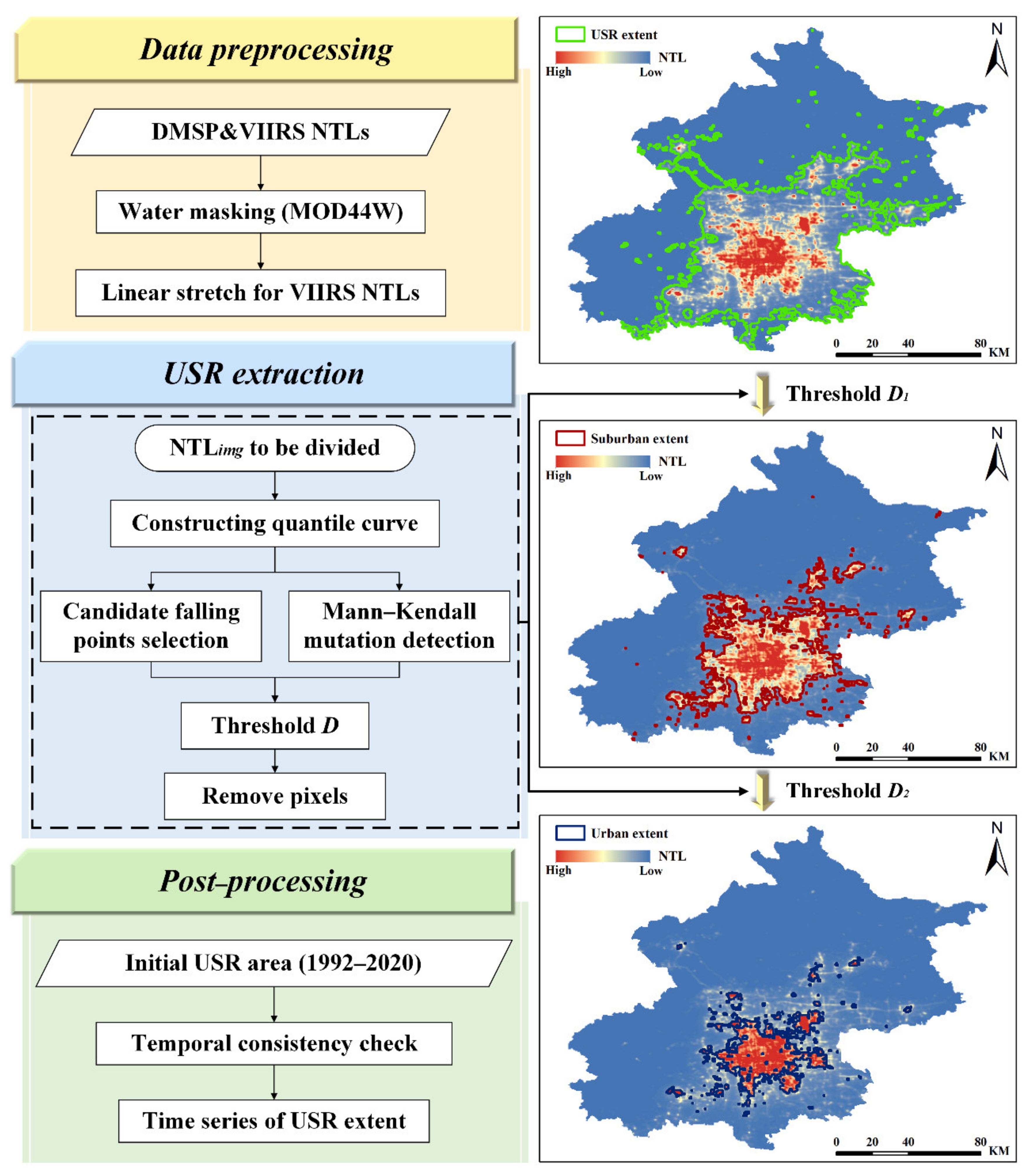
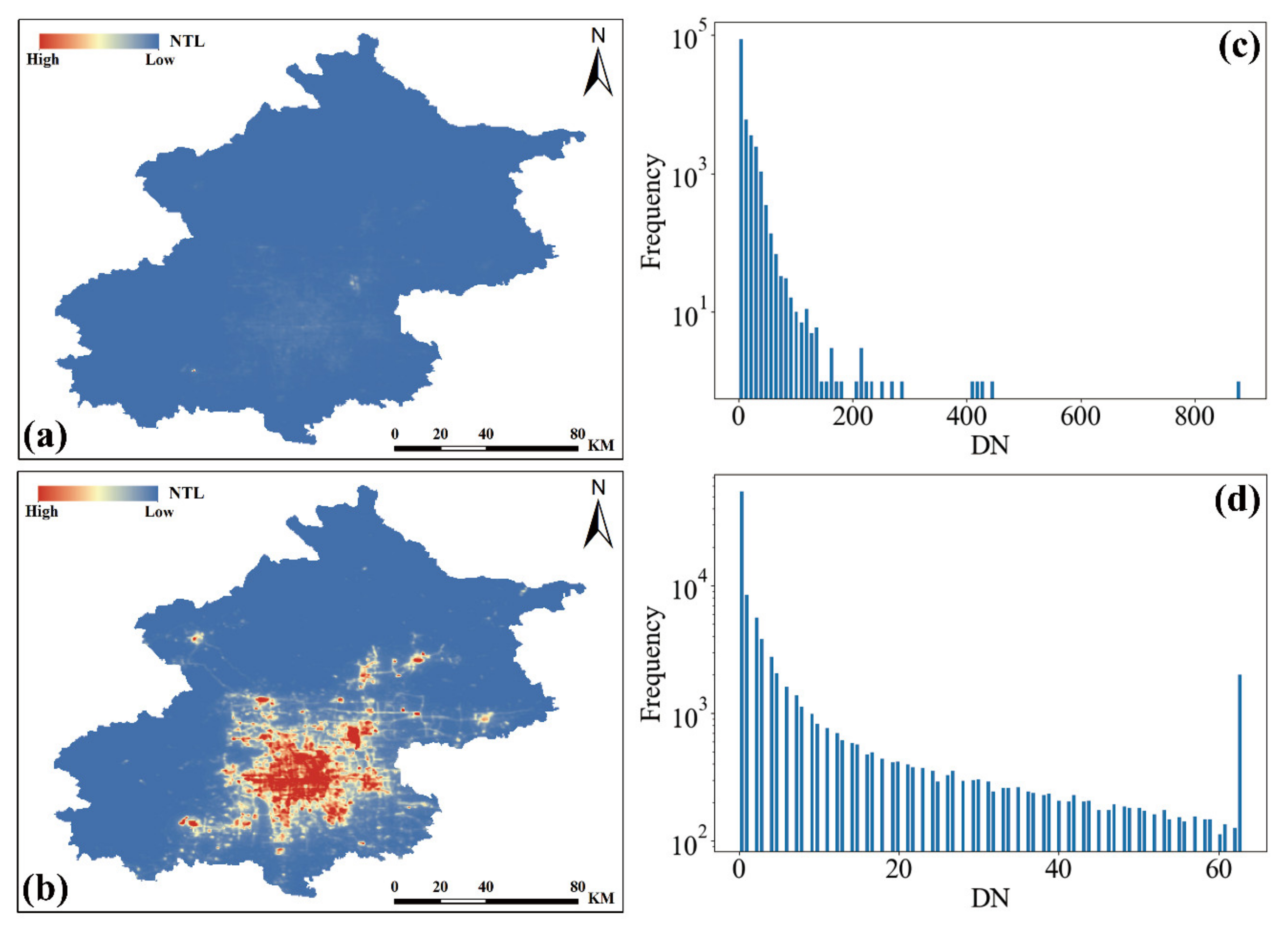
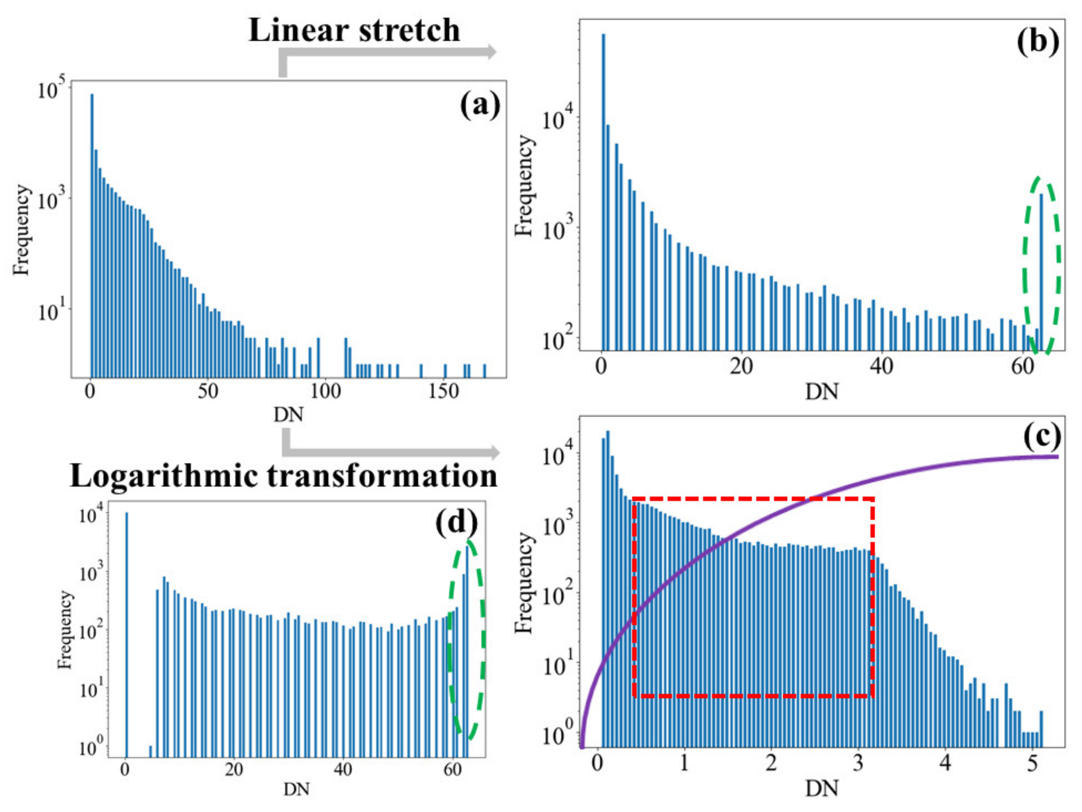
3.1. Data Preparation

The most basic definition of USR is a place where people live. That is, uninhabited places such as water and swaps should be removed first. To eliminate the pixels with nighttime light values greater than 0 caused by water, we first used the MODIS product MOD44W with a spatial resolution of 250 m to preprocess the original DMSP and VIIRS data. Compared with DMSP data with oversaturation, VIIRS data capture weaker nighttime lights and render them in a larger range of magnitude, which makes the pixel value of the most densely populated areas of human activity in the actual urban land far higher than that of the other urban land. Therefore, we performed a maximum–minimum (0–63) piecewise linear stretch on the initial VIIRS data to compress the exorbitant lighting values of some pixels in the actual urban land (Figure 2) to match the value ranges of DMSP/OLS data without changing the real USR distribution of VIIRS data. The piecewise linear stretch is expressed in the following equation:
X o u t p u t = 0 ,                                           X i n p u t Q 1 i n t X i n p u t Q 1 Q 2 Q 1 × 63 ,       Q 1 < X i n p u t < Q 2 63 ,                                     X i n p u t Q 2 ,
where Q 1 and Q 2 represent the 2nd percentile and 98th percentile of the input VIIRS data, respectively. X i n p u t means the value of each pixel in the input VIIRS data and X o u t p u t means the output value of the input pixel. The operator “int” is the antonomasia of the rounding function.

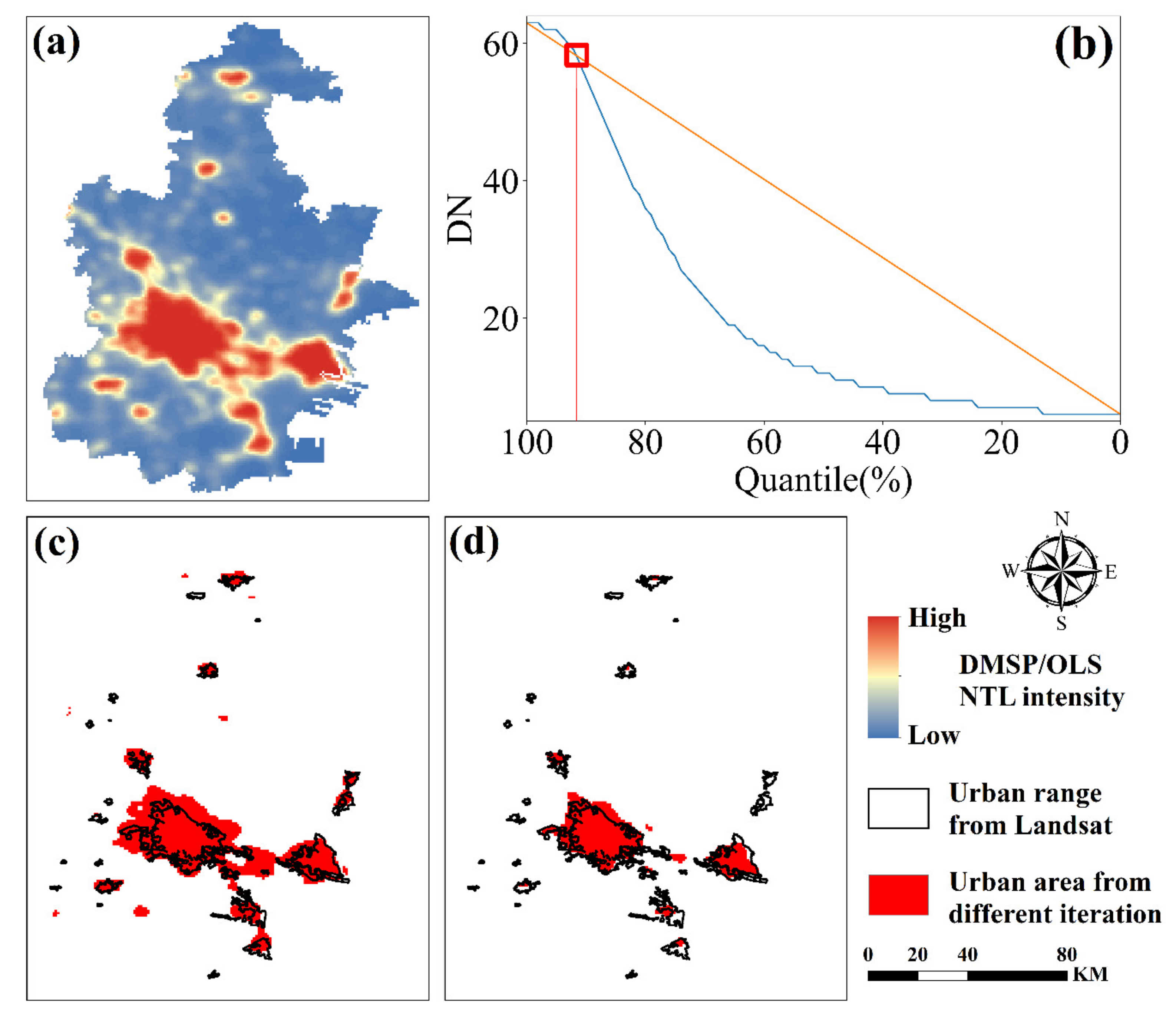
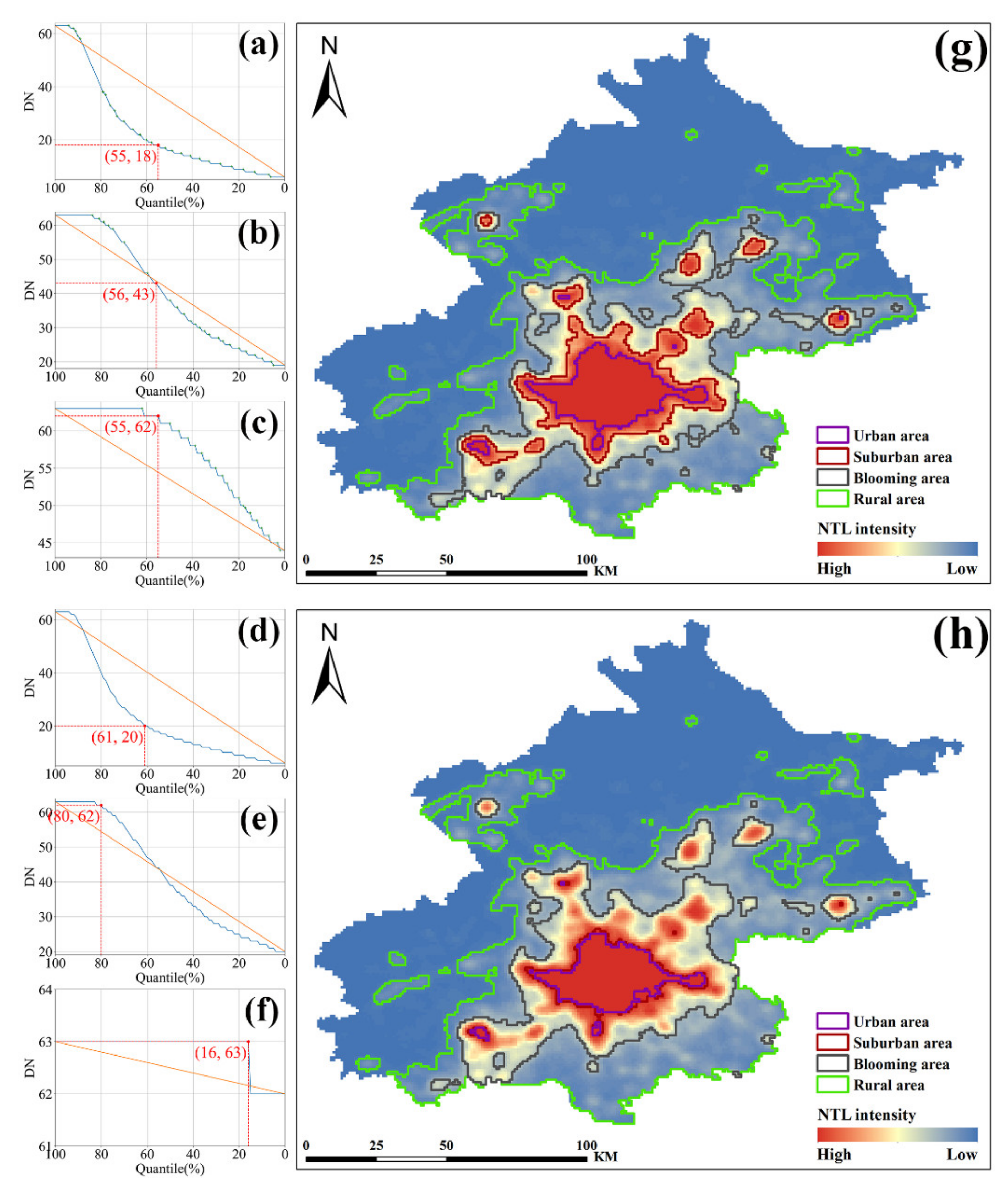
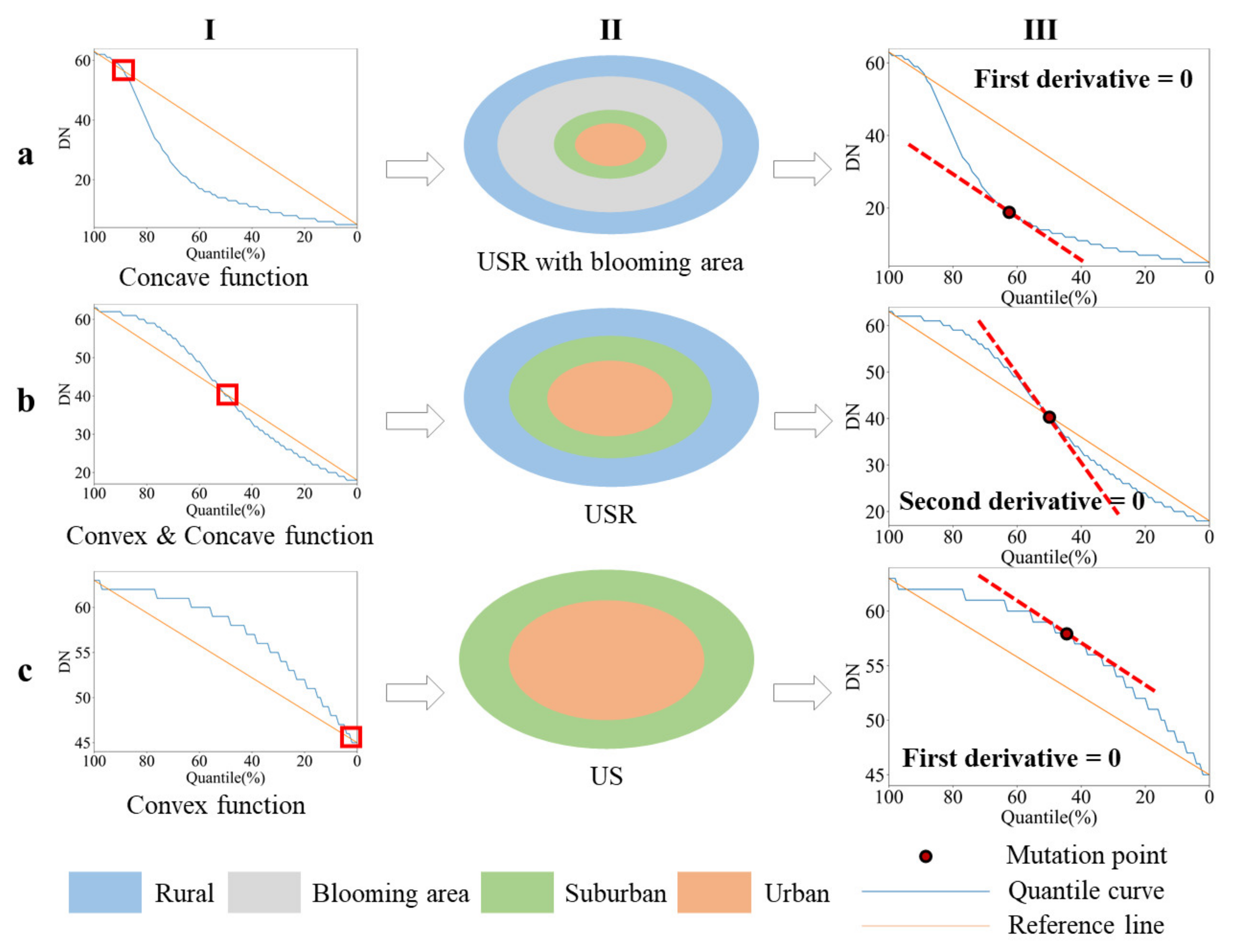
3.2. USR Extraction Based on Gradient Mutation Detection

We developed an innovative algorithm based on the gradient mutation detection of NTL images and the regulation of USR distribution to progressively determine the value of the thresholds between urban core, suburban, and rural areas. When the water area has already been removed, the remaining pixels with values larger than zero will still include areas where no people live because of the blooming effect of NTL images, especially in the DMSP data. To remove such unpopulated areas, we eliminated the pixels with values smaller than the 20th percentile of the DMSP data in the original DMSP data and the pixels with values smaller than the 5th percentile of the VIIRS data in the original VIIRS data because there are fewer blooming effects in the VIIRS data. Then, we assumed that all the remaining pixels belong to residential areas. This was then considered to be the whole USR extent for the next gradient mutation detection.
To fully recognize the gradient variation in the USR region extracted from NTL images, the whole USR extent was first used to construct a quantile curve that revealed the variation in NTL intensity with percentiles from 0 to 100 in the NTL image and along with the corresponding reference line directly connecting the two endpoints of the quantile curve [13]. Gradient mutation detection hypothesizes that the values of the pixels around the boundary lines between the urban core and suburban, and suburban and rural areas change rapidly and this leads to a sudden drop in the corresponding position of the quantile curve. For one potential extent of USR in the administrative region of a city, there can be several turning points corresponding to one sudden drop in the quantile curve. However, only the digital number (DN) values of two of them are needed, which will represent the threshold values of boundary lines segregating urban core and suburban or suburban and rural areas. The key to gradient mutation detection is determining the threshold values most efficiently.
To shorten the search time, we first established a list of candidate turning points based on the quantile curve to remove the redundant points. The two optimal threshold values of turning points can be considered as the mutation point in the quantile curve. In contrast to the perceptual determination with the maximum gap between the quantile curves and reference lines [13,23,32], the mutation point is redefined in this paper from the standpoint of derivatives. Based on the reference line, the quantile curve can be approximately regarded as a combination of a convex function and a concave function, the proportions of which in the whole quantile curve manifest the residential type of the input NTL image. This then determines where the mutation point lies (Figure 3). It is more significant to map USR than urban extent only. In this paper, we used a heuristic algorithm originating from the Mann–Kendall method, which is widely used for trend testing in hydrology [48,49], to determine the mutation point. The Mann–Kendall-inspired algorithm is expressed in the following equation:
s g n i = 1 ,   D i > D j 0 ,   D i D j ,   1 j i
S k = i = 1 k s g n i ,   2 k n
U F k = S k E S k V a r S k
  D i and D j represent the DN values of two neighboring points in the quantile curve. The number of the points in one quantile curve is n . The operator “ E ” is the antonomasia of calculating average value; The operator “ V a r ” is the antonomasia of calculating variance. The forward sequence U F k was computed by the formulas listed above with the input DN values ranking according to the percentile from 0 to 100, while the inverse sequence U B k was computed in the same way using the inverse DN values ranking according to the percentile from 100 to 0 as input. The mutation point of the original data was obtained by finding the intersection point of the forward and inverse sequences on the same abscissa. Figure 3 shows the three types of constructed quantile curves (column I), the specific USR structures corresponding to each quantile curve (column II), and the mutation points calculated by the Mann–Kendall-inspired algorithm (column III). When the quantile curve is regarded as a concave function (Figure 3(aⅠ)), it refers to the USR structure with blooming area (Figure 3(aⅡ)) and the point with the first derivative is zero on the quantile curve which is detected as the mutation point (Figure 3(aⅢ)); when the quantile curve is regarded as a combination of a convex function and a concave function (Figure 3(bⅠ)), it refers to the USR triad structure (Figure 3(bⅡ)) and the point with the second derivative is zero on the quantile curve is detected as the mutation point (Figure 3(bⅢ)); when the quantile curve is regarded as a convex function (Figure 3(cⅠ)), it refers to the urban core–suburban (US) structure (Figure 3(cⅡ)) and the point with the first derivative is zero on the quantile curve is detected as the mutation point (Figure 3(cⅢ)).
Combining all the steps mentioned above, the overall process of USR extraction can be divided into four major steps: (1) construct quantile curves based on the NTL image to be divided; (2) calculate all the candidate turning points in the quantile curve; (3) detect the mutation point using the heuristic algorithm originating from the Mann–Kendall method; and (4) determine the turning point with the closest DN value to that of the mutation point. According to the hypothesis of the three subcategories of the USR structure of cities varying greatly in population density and human activity intensity, this heuristic approach can retrieve urban core, suburban, and rural areas with two iterations. The first iteration separates the rural areas, and the second identifies the suburban areas, while the rest of the NTL image is recognized as the urban core. However, the blooming effect of the DMSP/OLS NTL data, which narrows the gap in the NTL intensity between the urban core and suburban areas in the cities with a low level of economic development in a specific year, makes it hard to distinguish the USR structure properly within two iterations when the inherent USR structure of cities was replaced by “urban core-suburban-blooming-rural” (USBR) NTL distribution in corresponding DMSP/OLS NTL images. To solve this problem, we used the percentile of the intersection point of the quantile curve and the reference line of the total USR range to determine whether the third iteration is needed to extract the real urban core (Figure 4). The USR range with a percentile of the intersection point greater than 70 is regarded as the rural-dominated type with fewer urban pixels, which is more likely to display the USBR NTL distribution. Thus, the second iteration separated the blooming area instead of the suburban area and the third iteration is needed.

3.3. Temporal Consistency Check

The time series DMSP NTL images acquired by different sensors lack time continuity due to the influence of many external factors, such as satellite orbit drift, along with the fact that the satellite sensors are not corrected by satellite radiometric correction. This will affect the identification of the DMSP NTL distribution and the number of iterations for USR extraction. Therefore, we first applied temporal filtering with a window size of 7 to revise the number of iterations for USR extraction for each city based on DMSP NTL imagery. Then, a temporal consistency check and logical reasoning modification based on the irreversibility of the urbanization process were employed for each pixel in both the DMSP and VIIRS USR ranges to obtain a more reliable USR-extent sequence with less temporal inconsistency from 1992 to 2020. A detailed description of the method can be found in Li et al. (2015).

4. Results

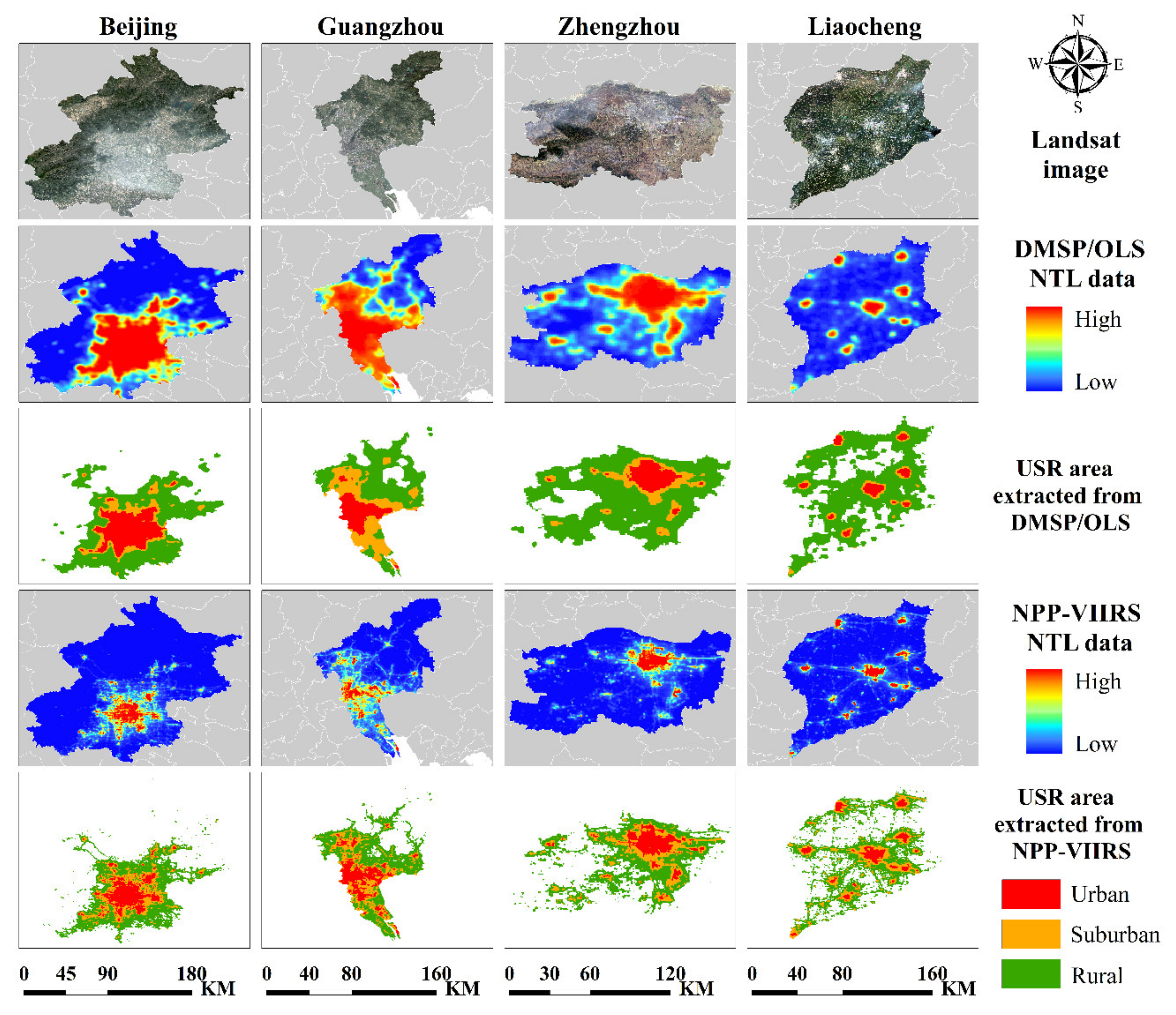
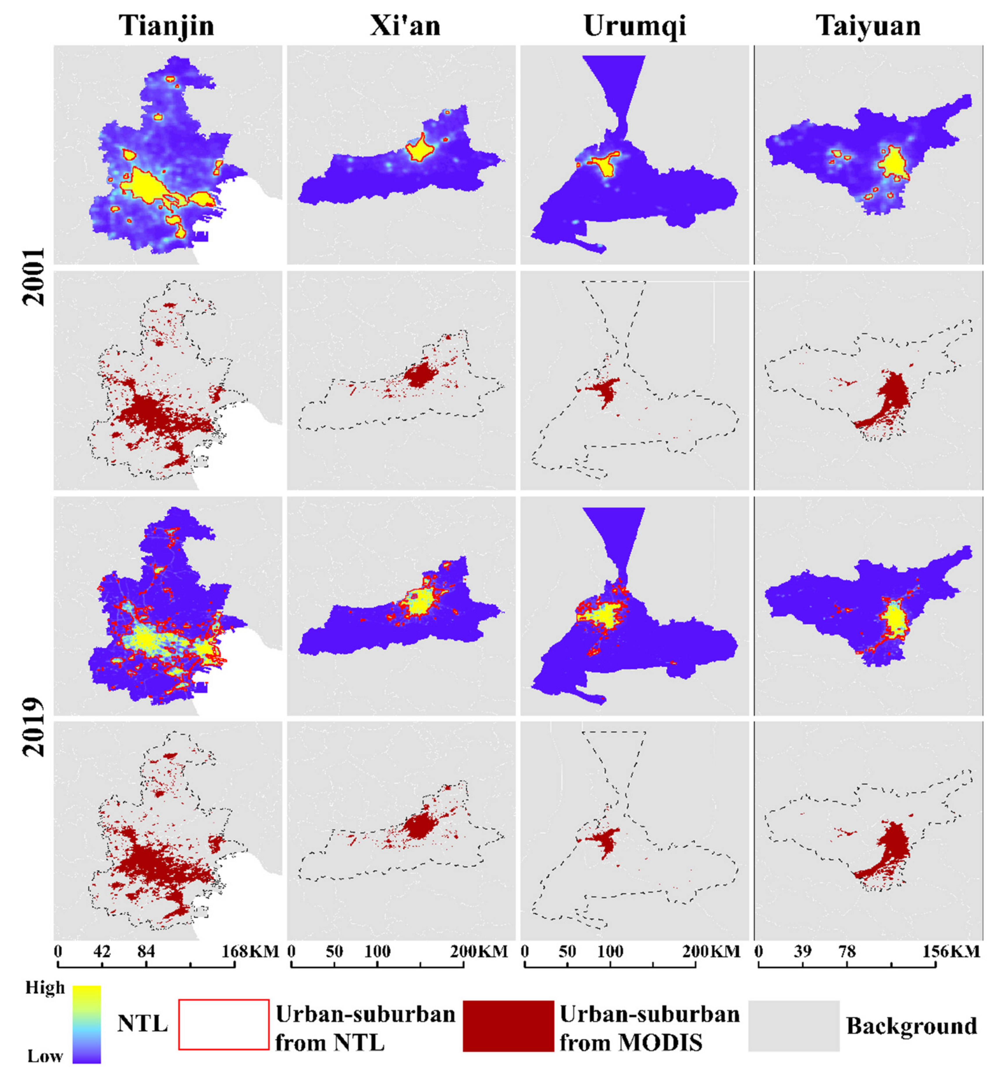
4.1. Performance of the Proposed Method on Different NTL Datasets

To validate the performance of the proposed method on different NTL datasets of DMSP and VIIRS, we chose the overlap datasets (2012–2013) to conduct both visual and quantitative evaluation. Figure 5 shows that the proposed method can effectively capture the spatial distribution of urban areas, suburban areas, and rural areas from different cities with various levels of urbanization and population sizes (supercity: Beijing; megacity: Guangzhou; large cities: Zhengzhou, Liaocheng) based on both DMSP and VIIRS NTL imagery. The urban extents retrieved from different NTL datasets present similar morphologies, such as bulked in Beijing and Guangzhou and dispersed in Liaocheng. The suburban extents retrieved from different NTL datasets all display as the adjacent areas of each urban core no matter what the pattern of city is. The rural extents extracted from different NTL datasets broadly share the same shape and distribution, while the areas of rural extents from DMSP are apparently larger than that from VIIRS due to the blooming effects of the DMSP.
Furthermore, we compared the USR results from two different NTL datasets (Table 3). The VIIRS result is more detailed because of its higher spatial resolution and small blooming effect. The four sample cities in Figure 5 show that the VIIRS dataset detected scattered urban areas around the core, which was missed by DMSP. Owing to the coarse resolution and the blooming effect, the DMSP dataset overestimated rural areas by polymerizing the transitional zones around several densely populated areas, which leads the area from VIIRS to be smaller than that from DMSP. However, the median deviation and average deviation between the urban and suburban results from DMSP and VIIRS were approximately 20%, and Pearson’s R reached 0.8, indicating the correlation between the urban and suburban results from DMSP and VIIRS. Notably, the median deviation and average deviation between the rural results from DMSP and VIIRS were reasonably high, as the rural areas with the dimmest night light were worst affected by the difference in spatial resolution between the DMSP and VIIRS NTL datasets. The inconsistency of the rural areas from different NTL datasets was caused by the coarse resolution and the blooming effect of DMSP/OLS. Overall, the comparison between the urban and suburban results from different NTL datasets shows a generally acceptable correlation.

4.2. Evaluations of Extracted USR Extent

To evaluate a consistent long-term series of USR extent, the spatial resolution of VIIRS NTL imagery was converted to be the same as that of DMSP NTL imagery. Considering that no reliable USR dataset has existed recently, the urban area in the land use map visual interpreted from Landsat imagery was used as an urban core for evaluations in this study. The built-up areas from MODIS land cover product MCD12Q1 were applied for the validation of the whole range of urban cores and suburban areas retrieved from consistent NTL datasets. Taking Wuhan city spanning 1992–2020 as an example (Figure 6), the extents of USR subcategories from NTL datasets show that urban area increased gradually in a reasonable way. To further quantitatively evaluate the performance of the proposed method in extracting urban cores, the overall accuracy (OA) and the kappa coefficient (KC) [50] were applied to 19 study cities with the visual interpretation results from Landsat imagery. With the average OA of all urban core extents retrieved from NTL imagery higher than 0.95 and the average KC reaching 0.6, the results of the proposed method for USR extraction show good spatial agreement with the urban area from Landsat imagery (see Table 4). Analyzing all the results through the entire period for each city, the urban core areas extracted from Taiyuan, Beijing, and Xi’an earn the best performance, with the top three average KCs all being greater than 0.7, while those from Sanya and Shangqiu performing the worst, with the average KCs being lower than 0.5. This indicates that the performance of the proposed method would be affected by the spatial pattern of the urban range itself. From the perspective of the level of urbanization and population size, the classification results of all the three supercities (Beijing, Shanghai, Tianjin) and the six large cities (Zhengzhou, Urumqi, Changchun, Qingdao, Datong, Taiyuan) are highly consistent with the average KC greater than 0.6, while those of the three medium-sized cities (Bengbu, Shangqiu, Yingkou), one large city (Liaocheng), and one small city (Sanya) are generally consistent. This can be explained by the lower proportion or the scattered form (Liaocheng) of the urban area in the city. For the five megacities (Guangzhou, Xi’an, Wuhan, Nanjing, Chengdu), some of the classification results are highly consistent with the average KCs larger than 0.6 and even reaching 0.7, while the others are generally consistent with the average KC approximately equal to 0.57. This reveals that both the population size and the spatial pattern of the city determined the urban extraction based on NTL datasets using a single-threshold method. From the perspective of annual NTL imagery, all the average KC of the classification results obtained from DMSP NTL imagery (1995, 2000, 2005, 2010) are greater than 0.6, and the extracted results based on the VIIRS dataset provided a maximum of 0.633 (2020) and a minimum of 0.577 (2015).
Figure 7 shows an example of the urban core and suburban areas extracted from the DMSP imagery (2001) and VIIRS imagery (2019) of four of the study cities (Tianjin, Xi’an, Urumqi, and Taiyuan) compared with the built-up areas from MODIS. It indicates good spatial consistency with the time series product. The results of linear fitting as shown in Figure 8 illustrate that the urban core and suburban areas extracted from DMSP imagery and VIIRS imagery are relatively consistent with the built-up areas from MODIS land cover product MCD12Q1, respectively, with the slope and the Pearson’s R values both being higher than 0.7. Meanwhile, the higher Pearson’s R values and lower bias of the linear regression equation composed of the VIIRS results and the MODIS product indicate that the urban core and suburban area extracted from the VIIRS dataset are closer to the MODIS-based built-up areas than the urban core and suburban area extracted from the DMSP dataset.

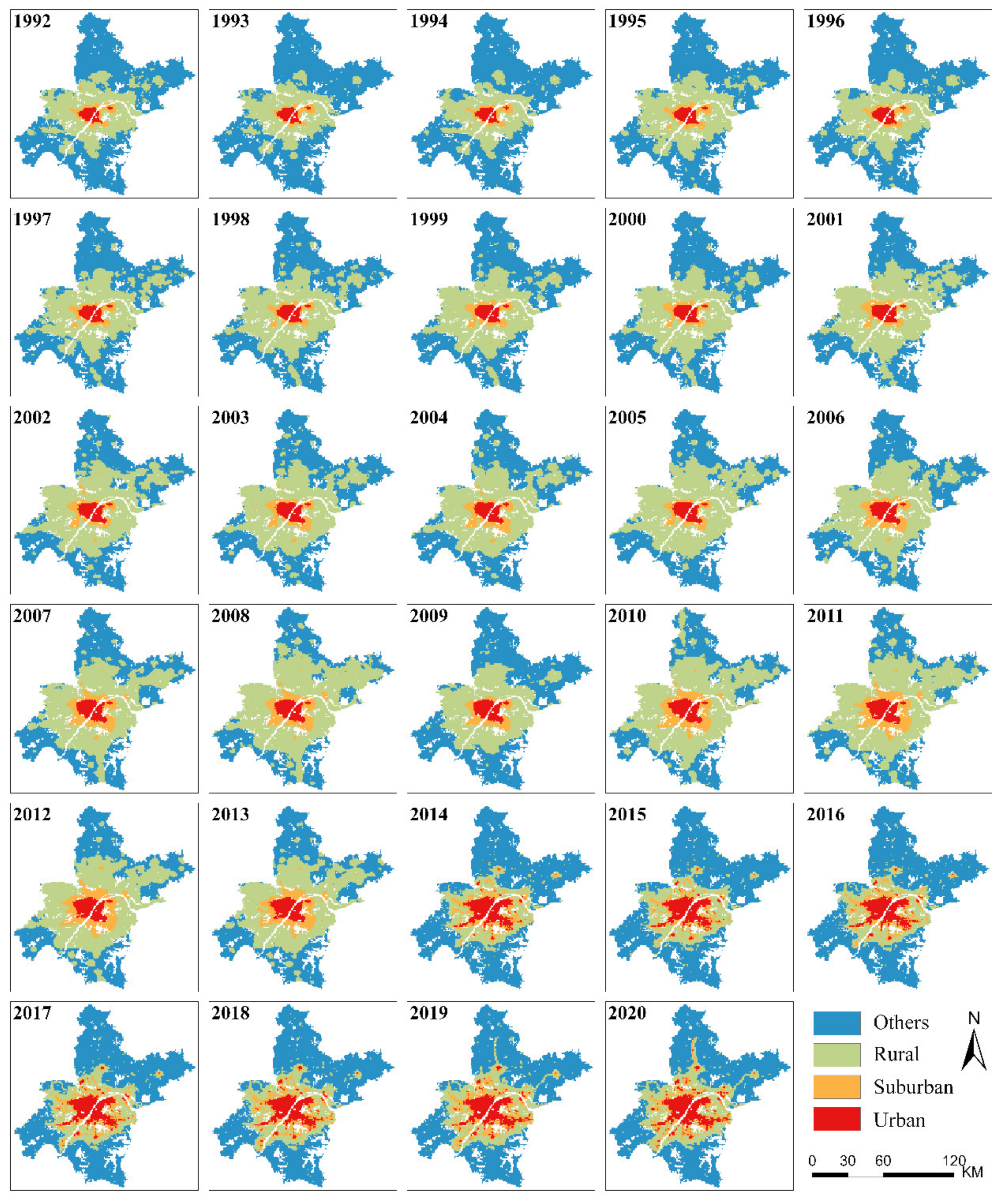
4.3. Spatiotemporal Analysis of Urbanization in the Study Area

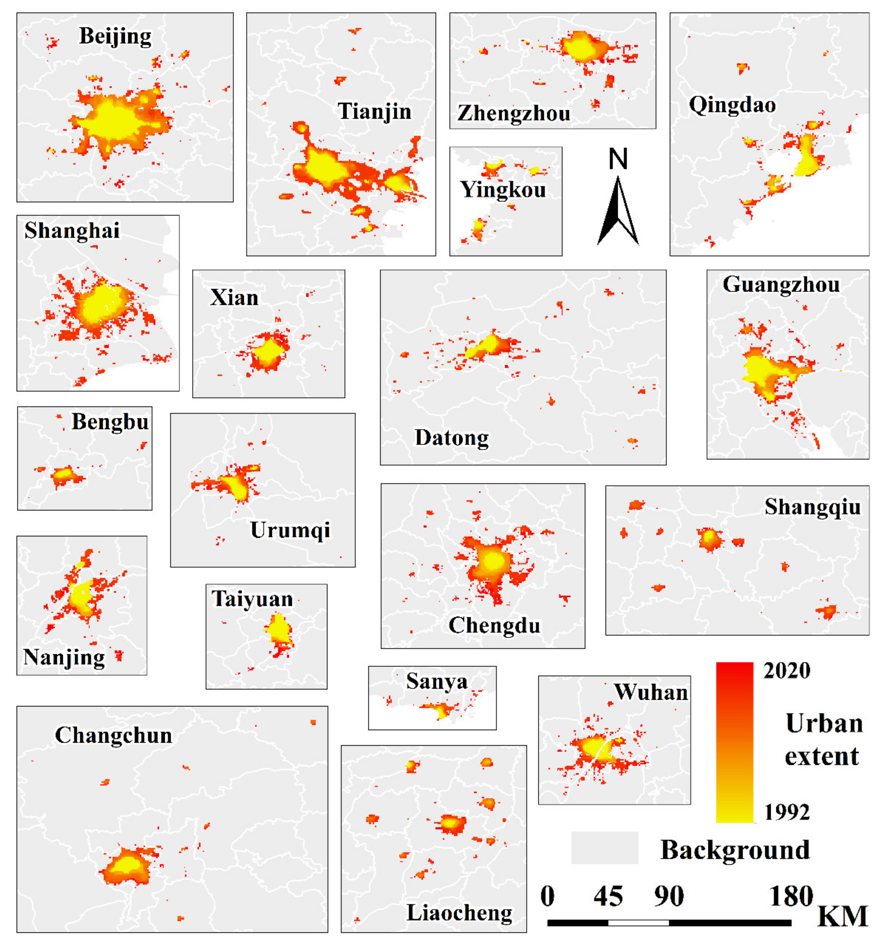
4.3.1. Urban Expansion throughout the Study Period

Obvious urbanization processes can be observed through the superposition of the urban areas retrieved from NTL data with diverse spatial patterns because of the different levels of socioeconomic development from 1992 to 2020. As shown in Figure 9, all the study cities have experienced notable urban expansion in recent decades with size, rate, and direction varying remarkably among different cities. Analyzing the expansion size of the cities, the three supercities (Beijing, Tianjin, and Shanghai) present a reasonable and noticeable urban growth with the top three increased areas, which are 1476 km2, 1479 km2, and 1275 km2, respectively. One of the large cities (Liaocheng) and one of the medium-sized cities (Shangqiu) have undergone the most numerous urban expansions compared to their urban areas in 1992, which attained growth rates of an urban expansion reaching 36 and 18, respectively. In addition, the directions of urban expansion also mark the difference in the urbanization process among different cities. This can be generally divided into two types: radiating outward from the center (type A) and radiating in a single direction (type B). For instance, the urban expansion occurring in Chengdu, Xi’an, and Nanjing displays a trend of expanding radially from the center outward, while the urban expansion of Datong, Taiyuan, and Sanya shows the tendency of expanding in a single direction, such as east, south, and north (Figure 10). This might be due to topographic factors.
From Table 5, the urban expansion of the supercities and megacities tends to be of type A, while that of some cities with smaller population sizes tends to be of type B. Only two of the supercities and megacities presented the urban expansion of type B because of geographical factors, while the other six presented the urban expansion of type A. Thus, the proportion of type A in supercities and megacities reached 75%. Correspondingly, two of the large cities and medium-sized cities presented the urban expansion of type A, as Liaocheng and Shangqiu are cities with multiple centers, while the other nine presented the urban expansion of type B. Thus, the proportion of type B in large cities, medium-sized cities, and small cities reached 82%. The percentage of the urban areas in 2020 transformed from rural areas in 1992 illustrated the degree and magnitude of urban expansion, which gradually increased as the population size of the city decreased.

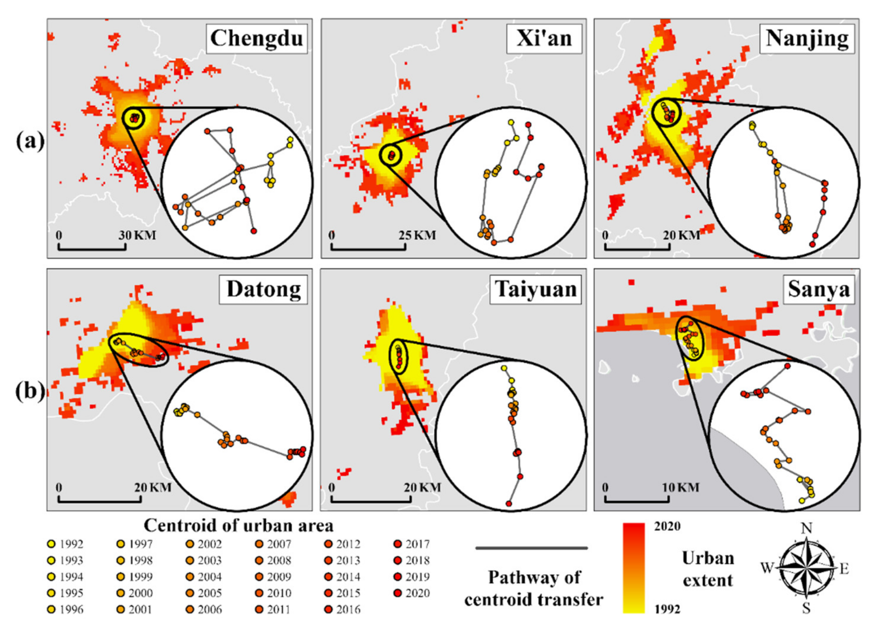
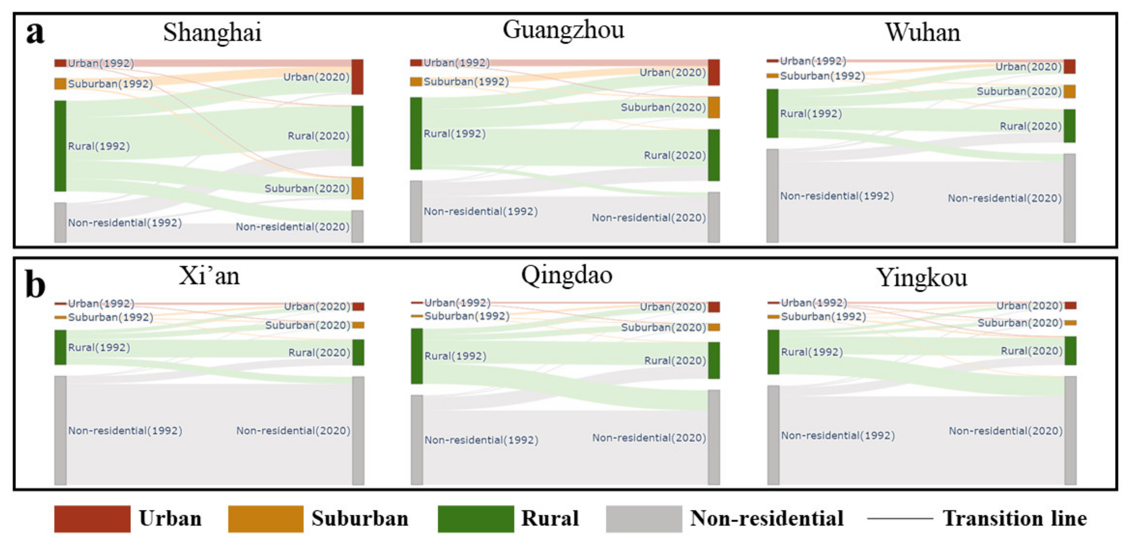
4.3.2. Transition Patterns of USR Interactions

In addition to the notable urban expansion, the spatial patterns of mutual transitions among the three USR subcategories also present an interesting tendency. Table 6 presents the part of the transition matrix of residential land use types from 1992 to 2020 for the study area, which illustrates that various conversion types into urban areas have taken place alongside the urban expansion. Almost all the main sources of urban areas in 2020 were rural areas in 1992, which indicates that profound and tremendous urbanization has occurred during the past few decades. Nevertheless, Taiyuan—one of the large cities with an urban resident population of more than 1 million and less than 5 million—has experienced less rapid urbanization compared with the urban areas in 1992 as the main sources of the urban area in 2020. According to the table, the degree and magnitude of urban expansion also vary among different cities with diverse population sizes. The urban expansion in Beijing, Shanghai, Tianjin, and Guangzhou—which are known as famous major metropolitan areas in China—eroded the rural areas at the lowest level, with a percentage of urban areas transformed from rural areas smaller than 0.5, while maintaining the urban areas at the highest level, with the percentage reaching an average of 0.243. As the population sizes of the cities decreased, the percentages of the urban areas in 2020 that transformed from rural and the other areas in 1992 increased, which illustrated that the transition pattern of urban expansion was related to the initial level of urbanization of the city.
The Sankey diagrams based on the land use transfer matrix between 1992 and 2020 provide a more intuitive way to analyze the characteristics of land use transfer in cities with different population sizes and economic locations. For example, Figure 11 shows the transformation of residential land use in six cities, which generally summarizes the situation of all cities. In Shanghai, Guangzhou, and Wuhan, the rural–urban and rural–suburban transformations top the list, and the proportion of them decreases progressively, indicating that these cities have experienced significant urbanization, as have other eastern and central supercities and megacities. In Xi’an, Qingdao, and Yingkou, the growth rates of urban and suburban areas were slower compared to the former, and rural and nonresidential areas still occupied the majority of the city. This represents the general situation of large cities and medium-sized cities in western and northeastern China.

5. Discussion

5.1. Less Adjustment of VIIRS NTL in Harmonized NTL Time Series Datasets

Long-term NTL time series data fill the gap of accessible data for retrieving time series of USR subcategories in a semiautomatic and more rapid way, among which the DMSP NTL imagery provides the data from 1992 to 2013, while the VIIRS NTL imagery makes the data spanning the years 2012–2020 available. However, there are some disadvantages to mapping USR extents using DMSP NTL data owing to the existing blooming and oversaturation effect [51], which exaggerates the extracted extent of suburban and rural areas compared with that from VIIRS NTL data. Using VIIRS NTL data of higher spatial resolution for USR extraction can improve the accuracies of the results to some extent (e.g., the average KC of urban areas extracted in Shangqiu from VIIRS NTL data reached 0.64, while that from DMSP NTL data was only 0.42 as shown in Table 4). In this study, we retrieved the USR based on their NTL gradient, which was directly displayed in VIIRS NTL datasets. Taking the processed VIIRS dataset proposed by Zhao et al. (2020) as an example, although over adjustments of VIIRS show sigmoid consistent temporal trends as DMSP NTL, it will lose the VIIRS details of USR with little area and introduce new uncertainty such as overestimation [39]. Figure 12 shows the comparison of the VIIRS variation after logarithmic transformation conducted by Zhao et al. and the adjusted VIIRS in this study. Compared to the histogram of the original VIIRS data (Figure 12a), the VIIRS variation after linear stretching in this paper basically follows the integral distribution pattern of the raw VIIRS imagery, while the VIIRS variation after logarithmic transformation shows a significant inconsistency with the raw VIIRS imagery in the middle- and low-DN areas (the red rectangle in Figure 12c). The logarithmic transformation indeed suppresses the sharp radiance jump between urban core areas and suburban and rural areas; however, the VIIRS radiance in suburban and rural areas tends to be homogenized. Compared to the histogram of the original DMSP data in the same year (Figure 12d), the VIIRS variation after linear stretching displays the same distribution in the high-DN areas (the green ellipses in Figure 12b,d), which might help to detect the urban core areas with high DN values. Hence, we propose that less adjustment of VIIRS to maintain its spatial and radiometric advantage is significant to USR retrieval for long-term consistent NTL datasets.

5.2. Uncertainty in the USR Extraction

The key feature of our approach for USR extraction lies in the combination of visualizing the gradient variation of NTL imagery using the quantile curve and mutation detection based on a heuristic algorithm originating from the Mann–Kendall method, which implied a hidden precondition that the result of the mutation detection must exactly match the corresponding DN values of the turning points obtained from the quantile curve. However, a spot of unmatching DN value pairs with gaps ranging from 1 to 4 was found during the experiments, and the solution to this was to seek out the turning point with the most proximate DN value to that of the mutation point; that is, the final DN value of the threshold was determined by the constructed quantile curve. On the other hand, determining the final DN value of the threshold based on a comparison of the DN values of the mutation point and the selected turning point, the results changed slightly. This is the optional fine-tuning for the USR extraction. The concrete practice of fine-tuning is to choose the DN value of the mutation point as the final threshold when the gap between the DN values of two points is greater than 1; otherwise, the DN value of the selected turning point is chosen as the final threshold. The results show that the fine-tuning technique can marginally ameliorate both overestimation (e.g., Changchun and Sanya in 2010) and underestimation (e.g., Wuhan in 2005) of the extracted urban area from DMSP datasets by acquiring a greater or smaller threshold.
The Mann–Kendall-based mutation point algorithm in this study is precise with mathematical implications. It consists of searching for the point at which the first or the second derivative is zero in the quantile curve according to different situations (Figure 3). Figure 13 shows the comparisons of extracted USR extent in Beijing with the quantile approach improved by Huang et al. to retrieve the extent of USR subcategories from NTL images, which just calculates the point on the quantile curve located farthest from the reference line [23]. Figure 13a–c are the threshold values of blooming, suburban, and urban areas using the Mann–Kendall-based mutation point algorithm, respectively, and Figure 13g displays the corresponding USR results. Meanwhile, Figure 13d–f are the threshold values of blooming, suburban, and urban areas based on the quantile approach, respectively, and Figure 13h displays the corresponding USR results. The quantile approach separating the USR subcategories based on the point on the quantile curve located farthest from the reference line can capture the point with the first derivative being zero when the patterns of NTL variations are the same as (d) or (f). However, it failed to identify the accurate mutation point regarding situations such as (e), as the retrieved suburban area was nearly the same as the retrieved urban area (Figure 13h), while the Mann–Kendall-based algorithm proposed in this paper succeeded in calculating the point with the second derivative of zero in the same situation (Figure 13b) and thus delineated the correct extent of the suburban area (Figure 13g).

5.3. Limitation

Compared with retrieving the urban core and suburban area from NTL datasets, there are challenges in mapping rural settlements based on NTL due to the discrete spatial distribution and the backward economy of rural areas. First, the basis of the close relation between NTL and human settlements lies in the NTL imagery seizing artificial lights at night, which are regarded as one of the most important signs of human activities. However, there are fewer detectable lights in rural settlements where people live than in metropolitan areas with higher economic development because of the traditional routine of “work at sunrise and rest at sunset” and the possible power shortage occurring in rural areas. Second, the scattered rural settlements are too small to be detected by the NTL sensors due to the coarse spatial resolution of NTL imagery (DMSP/OLS: 30 arc seconds, NPP-VIIRS: 15 arc seconds), leading to a resulting omission of part of the rural areas. Meanwhile, the rural areas for validation in 30 m or 100 m land use maps also exist as scattered areas, which further makes it difficult to compare with the extracted scope of rural areas from both DMSP and VIIRS NTL datasets when using the single-threshold method. In addition, some of the cities in China without the USR triad structure (e.g., Shenzhen did not have rural areas) need another specific strategy for urban core–suburban (US) extraction.
As for the data itself, the existing blooming effect and saturation problem of DMSP data might reduce the accuracy of the proposed method and lead to minor inconsistency with VIIRS data. For example, the blooming effect of DMSP NTL lightened the surroundings of aggregated rural settlements and thus obtained an overestimated scope of the whole area containing all rural settlements. As a result, the rural areas extracted from DMSP/OLS were apparently larger than that from NPP-VIIRS. Moreover, the linear stretch rounding the DN values of VIIRS as integers to match the data range of DMSP might probably miss the subtle changes of NTL intensity in low-DN regions. Therefore, the strategy of linear stretch for integrating DMSP and VIIRS NTL data can be further improved.

6. Conclusions

In this study, we developed an innovative approach based on the combination of NTL gradient variation and mutation detection using a heuristic algorithm inspired by the Mann–Kendall method. The goal is to map the extent of three USR subcategories from long-term NTL time series data spanning 1992–2020, which is set to meet the need for long time series of USR distributions. First, a maximum–minimum (0–63) piecewise linear stretch was applied for the VIIRS NTL data to match the value ranges of DMSP NTL data. Then, the USR extraction was processed through multiple iterations of the construction of the quantile curve and the detection of mutation points based on the quantile curve. Finally, a temporal consistency check was used to post-process the initial USR area to obtain a more consistent and reliable USR sequence from 1992 to 2020. Nineteen Chinese cities with different levels of urbanization and population sizes were chosen as the study area to verify the robustness and flexibility of the approach. The visual and quantitative evaluations of spatiotemporal consistency compared with the validation data indicate that the USR retrieval results showed good agreement with the land use map derived from Landsat images and the time series product from MODIS, with the average OA of overall urban extents higher than 0.95 and the average KC reaching 0.6.
According to the extracted USR distributions, the selected cities have experienced rapid and profound urbanization during the past decades. The rate, direction, and transition type of urban expansion vary among different cities with diverse levels of socioeconomic development. The growth rates of urban expansion in all the study cities range from 1.3 to the highest value of up to 36.5, and the average growth rate of the urban areas is 4.17. The directions of urban expansion can be generally divided into two types: radiating outward from the center (type A) and radiating in a single direction (type B). The urban expansion of the supercities and the megacities tends to be the former, while that of some cities with smaller population sizes tends to be the latter (Table 5). Specifically, Beijing, Tianjin, Wuhan, Chengdu, Xi’an, Nanjing, Liaocheng, and Shangqiu presented the urban expansion of type A, and the proportion of type A in all nineteen cities was 42%. On the other hand, Shanghai, Guangzhou, Zhengzhou, Changchun, Urumqi, Qingdao, Taiyuan, Datong, Bengbu, Yingkou, and Sanya presented the urban expansion of type B, and the proportion of type B in all 19 cities was 58%.
This study provides a new technique for mapping USR time series sequences using the integration of DMSP (1992–2013) and VIIRS (2014–2020) NTL data without altering the numerical distribution characteristics and spatial information features of the original VIIRS NTL. This makes it worthy of being promoted to the nationwide and even global scale. Notably, the blooming effect of DMSP NTL data led to an overestimation of the range of rural areas, which then generated an inconsistency between rural areas extracted from DMSP and VIIRS NTL since there was no blooming effect in the latter. Preprocessing of the low DN value region in DMSP NTL data referring to the corresponding area in VIIRS NTL data might help to improve the task of retrieving rural areas using the proposed approach. Moreover, the atmospheric factors might influence the extraction results of USR in relation to long-term time series data as the satellite measurements could be affected by aerosol concentration, humidity, and even lunar cycles [52,53,54,55,56]. Future implementation of the proposed method can also take the main atmospheric parameters into account.

Author Contributions

Conceptualization, Y.H. and M.C.; methodology, Y.H., J.Y. and M.C.; validation, Y.H., J.Y. and M.C.; data curation, J.Y. and C.W.; writing—original draft preparation, Y.H. and J.Y.; writing—review and editing, Y.H., J.Y., H.R. and Y.L.; funding acquisition, Y.H. All authors have read and agreed to the published version of the manuscript.

Funding

This research was funded by the National Natural Science Foundation of China (Grant NO. 41822104), the Strategic Priority Research Program of the Chinese Academy of Sciences (XDA19040402, XDA19040403), the National Key Research and Development Program of China (Grant NO. 2021YFC3002103), and the National Science and Technology Major Project of China’s High Resolution Earth Observation system (21-Y20B01-9001-19/22).

Conflicts of Interest

The authors declare no conflict of interest.

References

  1. Grimm, N.B.; Grove, J.G.; Pickett, S.T.A.; Redman, C.L. Integrated Approaches to Long-Term Studies of Urban Ecological Systems: Urban ecological systems present multiple challenges to ecologists—pervasive human impact and extreme heterogeneity of cities, and the need to integrate social and ecological approaches, concepts, and theory. BioScience 2000, 50, 571–584. [Google Scholar] [CrossRef] [Green Version]
  2. Wang, Y.; Li, X.; Kang, Y.; Chen, W.; Zhao, M.; Li, W. Analyzing the impact of urbanization quality on CO2 emissions: What can geographically weighted regression tell us? Renew. Sustain. Energy Rev. 2019, 104, 127–136. [Google Scholar] [CrossRef]
  3. Yang, J.; Yang, Y.; Sun, D.; Jin, C.; Xiao, X. Influence of urban morphological characteristics on thermal environment. Sustain. Cities Soc. 2021, 72, 103045. [Google Scholar] [CrossRef]
  4. Xie, P.; Yang, J.; Sun, W.; Xiao, X.; Cecilia Xia, J. Urban scale ventilation analysis based on neighborhood normalized current model. Sustain. Cities Soc. 2022, 80, 103746. [Google Scholar] [CrossRef]
  5. Wang, Q.; Wu, S.-D.; Zeng, Y.-E.; Wu, B.-W. Exploring the relationship between urbanization, energy consumption, and CO2 emissions in different provinces of China. Renew. Sustain. Energy Rev. 2016, 54, 1563–1579. [Google Scholar] [CrossRef]
  6. Luo, X.; Yang, J.; Sun, W.; He, B. Suitability of human settlements in mountainous areas from the perspective of ventilation: A case study of the main urban area of Chongqing. J. Clean. Prod. 2021, 310, 127467. [Google Scholar] [CrossRef]
  7. Ren, J.; Yang, J.; Zhang, Y.; Xiao, X.; Xia, J.C.; Li, X.; Wang, S. Exploring thermal comfort of urban buildings based on local climate zones. J. Clean. Prod. 2022, 340, 130744. [Google Scholar] [CrossRef]
  8. Yang, J.; Wang, Y.; Xue, B.; Li, Y.; Xiao, X.; Xia, J.; He, B. Contribution of urban ventilation to the thermal environment and urban energy demand: Different climate background perspectives. Sci. Total Environ. 2021, 795, 148791. [Google Scholar] [CrossRef]
  9. Chen, J. Rapid urbanization in China: A real challenge to soil protection and food security. Catena 2007, 69, 1–15. [Google Scholar] [CrossRef]
  10. Chen, M.; Ye, C.; Lu, D.; Sui, Y.; Guo, S. Cognition and construction of the theoretical connotations of new urbanization with Chinese characteristics. J. Geogr. Sci. 2019, 29, 1681–1698. [Google Scholar] [CrossRef] [Green Version]
  11. Ma, W.; Jiang, G.; Chen, Y.; Qu, Y.; Zhou, T.; Li, W. How feasible is regional integration for reconciling land use conflicts across the urban–rural interface? Evidence from Beijing–Tianjin–Hebei metropolitan region in China. Land Use Policy 2020, 92, 104433. [Google Scholar] [CrossRef]
  12. Sutton, P.C. A scale-adjusted measure of “Urban sprawl” using nighttime satellite imagery. Remote Sens. Environ. 2003, 86, 353–369. [Google Scholar] [CrossRef]
  13. Zhou, Y.; Li, X.; Asrar, G.R.; Smith, S.J.; Imhoff, M. A global record of annual urban dynamics (1992–2013) from nighttime lights. Remote Sens. Environ. 2018, 219, 206–220. [Google Scholar] [CrossRef]
  14. Cao, X.; Chen, J.; Imura, H.; Higashi, O. A SVM-based method to extract urban areas from DMSP-OLS and SPOT VGT data. Remote Sens. Environ. 2009, 113, 2205–2209. [Google Scholar] [CrossRef]
  15. Pandey, B.; Joshi, P.K.; Seto, K.C. Monitoring urbanization dynamics in India using DMSP/OLS night time lights and SPOT-VGT data. Int. J. Appl. Earth Obs. Geoinf. 2013, 23, 49–61. [Google Scholar] [CrossRef]
  16. Guindon, B.; Zhang, Y.; Dillabaugh, C. Landsat urban mapping based on a combined spectral–spatial methodology. Remote Sens. Environ. 2004, 92, 218–232. [Google Scholar] [CrossRef]
  17. Schneider, A.; Friedl, M.A.; Potere, D. Mapping global urban areas using MODIS 500-m data: New methods and datasets based on ‘urban ecoregions’. Remote Sens. Environ. 2010, 114, 1733–1746. [Google Scholar] [CrossRef]
  18. Demarchi, L.; Canters, F.; Chan, J.C.; Voorde, T.V.d. Multiple Endmember Unmixing of CHRIS/Proba Imagery for Mapping Impervious Surfaces in Urban and Suburban Environments. IEEE Trans. Geosci. Remote Sens. 2012, 50, 3409–3424. [Google Scholar] [CrossRef]
  19. Li, X.; Gong, P.; Liang, L. A 30-year (1984–2013) record of annual urban dynamics of Beijing City derived from Landsat data. Remote Sens. Environ. 2015, 166, 78–90. [Google Scholar] [CrossRef]
  20. Jacquin, A.; Misakova, L.; Gay, M. A hybrid object-based classification approach for mapping urban sprawl in periurban environment. Landsc. Urban Plan. 2008, 84, 152–165. [Google Scholar] [CrossRef]
  21. Herold, M.; Goldstein, N.C.; Clarke, K.C. The spatiotemporal form of urban growth: Measurement, analysis and modeling. Remote Sens. Environ. 2003, 86, 286–302. [Google Scholar] [CrossRef]
  22. Sawaya, K.E.; Olmanson, L.G.; Heinert, N.J.; Brezonik, P.L.; Bauer, M.E. Extending satellite remote sensing to local scales: Land and water resource monitoring using high-resolution imagery. Remote Sens. Environ. 2003, 88, 144–156. [Google Scholar] [CrossRef]
  23. Huang, Y.; Wu, C.; Chen, M.; Yang, J.; Ren, H. A Quantile Approach for Retrieving the “Core Urban-Suburban-Rural” (USR) Structure Based on Nighttime Light. Remote Sens. 2020, 12, 4179. [Google Scholar] [CrossRef]
  24. Levin, N.; Kyba, C.C.M.; Zhang, Q.; Sánchez de Miguel, A.; Román, M.O.; Li, X.; Portnov, B.A.; Molthan, A.L.; Jechow, A.; Miller, S.D.; et al. Remote sensing of night lights: A review and an outlook for the future. Remote Sens. Environ. 2020, 237, 111443. [Google Scholar] [CrossRef]
  25. Elvidge, C.D.; Imhoff, M.L.; Baugh, K.E.; Hobson, V.R.; Nelson, I.; Safran, J.; Dietz, J.B.; Tuttle, B.T. Night-time lights of the world: 1994–1995. ISPRS J. Photogramm. Remote Sens. 2001, 56, 81–99. [Google Scholar] [CrossRef]
  26. Elvidge, C.D.; Baugh, K.E.; Dietz, J.B.; Bland, T.; Sutton, P.C.; Kroehl, H.W. Radiance Calibration of DMSP-OLS Low-Light Imaging Data of Human Settlements. Remote Sens. Environ. 1999, 68, 77–88. [Google Scholar] [CrossRef]
  27. Croft, T. Nighttime Images of the Earth from Space. Sci. Am. 1978, 239, 86–98. [Google Scholar] [CrossRef]
  28. Song, Y.; Huang, B.; Cai, J.; Chen, B. Dynamic assessments of population exposure to urban greenspace using multi-source big data. Sci. Total Environ. 2018, 634, 1315–1325. [Google Scholar] [CrossRef]
  29. Li, X.; Zhao, L.; Li, D.; Xu, H. Mapping Urban Extent Using Luojia 1-01 Nighttime Light Imagery. Sensors 2018, 18, 3665. [Google Scholar] [CrossRef] [Green Version]
  30. Shi, K.; Huang, C.; Yu, B.; Yin, B.; Huang, Y.; Wu, J. Evaluation of NPP-VIIRS night-time light composite data for extracting built-up urban areas. Remote Sens. Lett. 2014, 5, 358–366. [Google Scholar] [CrossRef]
  31. Small, C.; Pozzi, F.; Elvidge, C. Spatial analysis of global urban extent from DMSP-OLS night lights. Remote Sens. Environ. 2005, 96, 277–291. [Google Scholar] [CrossRef]
  32. Zhao, M.; Zhou, Y.; Li, X.; Cheng, W.; Zhou, C.; Ma, T.; Li, M.; Huang, K. Mapping urban dynamics (1992–2018) in Southeast Asia using consistent nighttime light data from DMSP and VIIRS. Remote Sens. Environ. 2020, 248, 111980. [Google Scholar] [CrossRef]
  33. Su, Y.; Chen, X.; Wang, C.; Zhang, H.; Liao, J.; Ye, Y.; Wang, C. A new method for extracting built-up urban areas using DMSP-OLS nighttime stable lights: A case study in the Pearl River Delta, southern China. GIScience Remote Sens. 2015, 52, 218–238. [Google Scholar] [CrossRef]
  34. Zhou, Y.; Smith, S.J.; Elvidge, C.D.; Zhao, K.; Thomson, A.; Imhoff, M. A cluster-based method to map urban area from DMSP/OLS nightlights. Remote Sens. Environ. 2014, 147, 173–185. [Google Scholar] [CrossRef]
  35. Sutton, P.; Roberts, D.; Elvidge, C.; Baugh, K. Census from Heaven: An estimate of the global human population using night-time satellite imagery. Int. J. Remote Sens. 2001, 22, 3061–3076. [Google Scholar] [CrossRef]
  36. Ma, T.; Zhou, Y.; Zhou, C.; Haynie, S.; Pei, T.; Xu, T. Night-time light derived estimation of spatio-temporal characteristics of urbanization dynamics using DMSP/OLS satellite data. Remote Sens. Environ. 2015, 158, 453–464. [Google Scholar] [CrossRef]
  37. Zheng, Q.; Weng, Q.; Wang, K. Developing a new cross-sensor calibration model for DMSP-OLS and Suomi-NPP VIIRS night-light imageries. ISPRS J. Photogramm. Remote Sens. 2019, 153, 36–47. [Google Scholar] [CrossRef]
  38. Zhao, M.; Zhou, Y.; Li, X.; Cao, W.; He, C.; Yu, B.; Li, X.; Elvidge, C.D.; Cheng, W.; Zhou, C. Applications of Satellite Remote Sensing of Nighttime Light Observations: Advances, Challenges, and Perspectives. Remote Sens. 2019, 11, 1971. [Google Scholar] [CrossRef] [Green Version]
  39. Zhao, M.; Zhou, Y.; Li, X.; Zhou, C.; Cheng, W.; Li, M.; Huang, K. Building a Series of Consistent Night-Time Light Data (1992–2018) in Southeast Asia by Integrating DMSP-OLS and NPP-VIIRS. IEEE Trans. Geosci. Remote Sens. 2020, 58, 1843–1856. [Google Scholar] [CrossRef]
  40. Yu, B.; Tang, M.; Wu, Q.; Yang, C.; Deng, S.; Shi, K.; Peng, C.; Wu, J.; Chen, Z. Urban Built-Up Area Extraction From Log- Transformed NPP-VIIRS Nighttime Light Composite Data. IEEE Geosci. Remote Sens. Lett. 2018, 15, 1279–1283. [Google Scholar] [CrossRef]
  41. Li, X.; Zhou, Y.; Zhao, M.; Zhao, X. A harmonized global nighttime light dataset 1992–2018. Sci. Data 2020, 7, 168. [Google Scholar] [CrossRef]
  42. Kendall, M.G. Rank Correlation Methods. Br. J. Psychol. 1990, 25, 86–91. [Google Scholar] [CrossRef]
  43. Mann, H.B. Nonparametric Tests Against Trend. Econometrica 1945, 13, 245–259. [Google Scholar] [CrossRef]
  44. Elvidge, C.D.; Zhizhin, M.; Ghosh, T.; Hsu, F.-C.; Taneja, J. Annual Time Series of Global VIIRS Nighttime Lights Derived from Monthly Averages: 2012 to 2019. Remote Sens. 2021, 13, 922. [Google Scholar] [CrossRef]
  45. Elvidge, C.D.; Ziskin, D.; Baugh, K.E.; Tuttle, B.T.; Ghosh, T.; Pack, D.W.; Erwin, E.H.; Zhizhin, M. A Fifteen Year Record of Global Natural Gas Flaring Derived from Satellite Data. Energies 2009, 2, 595–622. [Google Scholar] [CrossRef]
  46. Xu, X.L.; Liu, J.Y.; Zhang, S.W.; Li, R.D.; Yan, C.Z.; Wu, S.X. China Multi-period Land Use Land Cover Remote Sensing Monitoring Data Set (CNLUCC). Data Registration and Publishing System of the Resource and Environmental Science Data Center of the Chinese Academy of Sciences. 2018. Available online: http://www.resdc.cn/DOI (accessed on 15 October 2021).
  47. Friedl, M.A.; Sulla-Menashe, D.; Tan, B.; Schneider, A.; Ramankutty, N.; Sibley, A.; Huang, X. MODIS Collection 5 global land cover: Algorithm refinements and characterization of new datasets. Remote Sens. Environ. 2010, 114, 168–182. [Google Scholar] [CrossRef]
  48. Dinpashoh, Y.; Jhajharia, D.; Fakheri-Fard, A.; Singh, V.P.; Kahya, E. Trends in reference crop evapotranspiration over Iran. J. Hydrol. 2011, 399, 422–433. [Google Scholar] [CrossRef]
  49. Gocic, M.; Trajkovic, S. Analysis of changes in meteorological variables using Mann-Kendall and Sen’s slope estimator statistical tests in Serbia. Glob. Planet. Chang. 2013, 100, 172–182. [Google Scholar] [CrossRef]
  50. Cohen, J. A Coefficient of Agreement for Nominal Scales. Educ. Psychol. Meas. 1960, 20, 37–46. [Google Scholar] [CrossRef]
  51. Liu, Z.; He, C.; Zhang, Q.; Huang, Q.; Yang, Y. Extracting the dynamics of urban expansion in China using DMSP-OLS nighttime light data from 1992 to 2008. Landsc. Urban Plan. 2012, 106, 62–72. [Google Scholar] [CrossRef]
  52. Cao, C.; Zhang, B.; Xia, F.; Bai, Y. Exploring VIIRS Night Light Long-Term Time Series with CNN/SI for Urban Change Detection and Aerosol Monitoring. Remote Sens. 2022, 14, 3126. [Google Scholar] [CrossRef]
  53. Fiorentin, P.; Cavazzani, S.; Ortolani, S.; Bertolo, A.; Binotto, R. Instrument assessment and atmospheric phenomena in relation to the night sky brightness time series. Measurement 2022, 191, 110823. [Google Scholar] [CrossRef]
  54. Cavazzani, S.; Ortolani, S.; Bertolo, A.; Binotto, R.; Fiorentin, P.; Carraro, G.; Zitelli, V. Satellite measurements of artificial light at night: Aerosol effects. Mon. Not. R. Astron. Soc. 2020, 499, 5075–5089. [Google Scholar] [CrossRef]
  55. Sawyer, V.; Levy, R.C.; Mattoo, S.; Cureton, G.; Shi, Y.; Remer, L.A. Continuing the MODIS Dark Target Aerosol Time Series with VIIRS. Remote Sens. 2020, 12, 308. [Google Scholar] [CrossRef] [Green Version]
  56. Kocifaj, M.; Bará, S. Aerosol characterization using satellite remote sensing of light pollution sources at night. Mon. Not. R. Astron. Soc. Lett. 2020, 495, L76–L80. [Google Scholar] [CrossRef] [Green Version]
Figure 1. Flow chart for USR extraction from NTL datasets.
Remotesensing 14 03642 g001
Figure 2. Comparison of VIIRS data before (a) and after (b) linear stretch. Histograms of the VIIRS data before (c) and after (d) linear stretch.
Remotesensing 14 03642 g002
Figure 3. Schematic diagram of the gradient mutation detection for USR extraction. Quantile curve (aI) of the USR structure with blooming area (aII) and the corresponding mutation point with the first derivative is zero (aIII). Quantile curve (bI) of the USR structure (bII) and the corresponding mutation point with the second derivative is zero (bIII). Quantile curve (cI) of the US structure (cII) and the corresponding mutation point with the first derivative is zero (cIII).
Remotesensing 14 03642 g003
Figure 4. A schematic diagram of the third iteration for USR extraction. (a) A sample DMSP NTL image in Tianjin. (b) The first quantile curve conducted based on the image with the quantile value of the intersection point higher than 70%. (c) Extracted urban area from the second iteration. (d) Extracted urban area from the third iteration.
Remotesensing 14 03642 g004
Figure 5. A comparison of urban areas extracted from DMSP and VIIRS in 2012.
Remotesensing 14 03642 g005
Figure 6. Extent of USR subcategories in Wuhan spanning 1992–2020.
Remotesensing 14 03642 g006
Figure 7. Examples of the urban core and suburban areas extracted from the DMSP imagery (2001) and VIIRS imagery (2019).
Remotesensing 14 03642 g007
Figure 8. Comparisons of urban–suburban areas from NTL and MODIS. The blue dots represent the comparisons of urban–suburban areas from DMSP and MODIS spanning 2001–2013, and VIIRS and MODIS spanning 2012–2019.
Remotesensing 14 03642 g008
Figure 9. Urban expansion of all cities spanning 1992–2020.
Remotesensing 14 03642 g009
Figure 10. Examples of two types of urban expansion, (a) radiating outward from the center, and (b) radiating in a single direction.
Remotesensing 14 03642 g010
Figure 11. Examples of two situations of residential land transformation. (a) Representation for eastern and central supercities and megacities. (b) Representation for large cities and medium-sized cities in western and northeastern China.
Remotesensing 14 03642 g011
Figure 12. Comparison of the VIIRS variation after linear stretch (b) and the VIIRS variation after logarithmic transformation (c). (a) Histogram of the original VIIRS data. (d) Histogram of the original DMSP data.
Remotesensing 14 03642 g012
Figure 13. Comparisons of extracted USR extent in Beijing with the quantile approach. (ac) are the threshold values of blooming, suburban, and urban areas using the Mann–Kendall-based mutation point algorithm, respectively, and (g) displays the corresponding USR results. (df) are the threshold values of blooming, suburban, and urban areas based on the quantile approach, respectively, and (h) displays the corresponding USR results.
Remotesensing 14 03642 g013
Table 1. Basic information of the 19 cities.
City ScaleCityPopulation Size (10,000 Persons)Economic Location
SupercityShanghai2428.14 Eastern
Beijing1916.40 Eastern
Tianjin1174.44 Eastern
MegacityChengdu760.63 Western
Guangzhou719.14 Eastern
Nanjing644.84 Eastern
Xi’an643.50 Western
Wuhan611.30 Central
Large cityQingdao433.94 Eastern
Zhengzhou416.64 Central
Changchun362.09 Northeastern
Taiyuan301.93 Central
Urumqi225.65 Western
Datong122.98 Central
Liaocheng114.59 Eastern
Medium-sized cityShangqiu96.38 Central
Bengbu82.70 Central
Yingkou77.70 Northeastern
Small citySanya32.69 Eastern
Table 2. Detailed information on the data used.
Satellite/SensorProductDataset TypeAvailable PeriodSpatial Resolution
DMSP/OLSStable lightTime series NTL dataset1992–2013 Annually30 arc second (~1000 m at the Equator)
NPP-VIIRSAnnual VNL V2Time series NTL dataset2012–2020 Annually15 arc second (~500 m at the Equator)
MODISMOD44WWater mask2000–2015 Annually250 m
MODISMCD12Q1LUCC2001–2019 Annually500 m
Landsat TM/OLI100 m Land useLUCC1995/2000/2005/2010/2015/2020100 m
Table 3. Comparisons of USR results from DMSP and VIIRS.
Residential TypeMedian DeviationAverage DeviationPearson’s R
2012Urban23.87%23.63%0.846
Suburban17.15%24.14%0.853
Rural51.84%44.64%0.682
2013Urban21.76%21.74%0.873
Suburban26.62%28.94%0.762
Rural45.14%44.46%0.781
Table 4. Accuracies of extracted urban from different cities based on NTL imagery (OA: overall accuracy, KC: kappa coefficient).
Year199520002005201020152020Average
CityOAKCOAKCOAKCOAKCOAKCOAKCOAKappa
Beijing0.975 0.748 0.972 0.735 0.963 0.713 0.951 0.699 0.941 0.676 0.943 0.709 0.958 0.713
Shanghai0.949 0.687 0.947 0.690 0.925 0.662 0.925 0.660 0.879 0.596 0.853 0.625 0.913 0.653
Tianjin0.969 0.653 0.965 0.631 0.957 0.654 0.956 0.639 0.906 0.540 0.921 0.645 0.945 0.627
Guangzhou0.960 0.621 0.957 0.612 0.931 0.622 0.929 0.634 0.915 0.633 0.903 0.617 0.933 0.623
Xi’an0.991 0.762 0.991 0.773 0.987 0.727 0.985 0.711 0.971 0.633 0.967 0.646 0.982 0.709
Wuhan0.978 0.593 0.978 0.620 0.971 0.595 0.966 0.575 0.947 0.549 0.930 0.484 0.962 0.569
Nanjing0.970 0.581 0.963 0.568 0.954 0.570 0.940 0.513 0.918 0.545 0.923 0.678 0.945 0.576
Chengdu0.987 0.552 0.984 0.552 0.978 0.596 0.971 0.587 0.955 0.559 0.946 0.595 0.970 0.574
Zhengzhou0.981 0.661 0.979 0.658 0.969 0.672 0.963 0.647 0.948 0.616 0.931 0.618 0.962 0.645
Urumqi0.991 0.616 0.988 0.581 0.988 0.599 0.989 0.689 0.983 0.680 0.981 0.727 0.987 0.649
Changchun0.991 0.552 0.992 0.588 0.991 0.619 0.985 0.623 0.983 0.663 0.985 0.767 0.988 0.636
Qingdao0.981 0.644 0.978 0.636 0.969 0.616 0.968 0.618 0.959 0.608 0.957 0.679 0.969 0.634
Datong0.994 0.646 0.993 0.622 0.993 0.681 0.989 0.630 0.976 0.493 0.977 0.613 0.987 0.614
Taiyuan0.985 0.736 0.984 0.731 0.982 0.720 0.981 0.719 0.977 0.697 0.972 0.710 0.980 0.719
Bengbu0.994 0.576 0.993 0.521 0.993 0.591 0.986 0.480 0.972 0.467 0.970 0.487 0.985 0.520
Shangqiu0.992 0.345 0.990 0.365 0.988 0.407 0.988 0.562 0.977 0.592 0.980 0.707 0.986 0.496
Yingkou0.987 0.580 0.986 0.585 0.982 0.519 0.977 0.519 0.964 0.440 0.965 0.573 0.977 0.536
Liaocheng0.991 0.471 0.989 0.457 0.984 0.535 0.985 0.677 0.966 0.590 0.968 0.692 0.980 0.570
Sanya0.990 0.495 0.989 0.531 0.978 0.377 0.965 0.368 0.946 0.384 0.940 0.460 0.968 0.436
Average0.982 0.606 0.980 0.603 0.973 0.604 0.968 0.608 0.952 0.577 0.948 0.633 0.967 0.605
Table 5. Types of urban expansion (Type A: radiating outward from the center, Type B: radiating in a single direction).
City ScaleCityPopulation SizeEconomic LocationType of Urban Expansion
SupercityBeijingHigher than 10 million EasternA
ShanghaiEasternB
TianjinEasternA
MegacityGuangzhouHigher than 5 million less than 10 millionEasternB
WuhanCentralA
ChengduWesternA
Xi’anWesternA
NanjingEasternA
Large cityZhengzhouHigher than 1 million less than 5 millionCentralB
ChangchunNortheasternB
UrumqiWesternB
QingdaoEasternB
TaiyuanCentralB
DatongCentralB
LiaochengEasternA
Medium-sized cityBengbuHigher than 500 thousand less than 1 millionCentralB
YingkouNortheasternB
ShangqiuCentralA
Small citySanyaLess than 500 thousandEasternB
Table 6. Percentage of transition area from different residential types to urban area in 2020 (%).
Residential TypeUrbanSuburbanRuralNon-Residential
Beijing0.285 0.271 0.436 0.008
Shanghai0.211 0.263 0.475 0.051
Tianjin0.217 0.265 0.496 0.023
Guangzhou0.259 0.264 0.456 0.021
Xi’an0.270 0.224 0.506 0.000
Wuhan0.198 0.238 0.528 0.036
Nanjing0.195 0.244 0.536 0.026
Chengdu0.077 0.088 0.554 0.281
Zhengzhou0.180 0.143 0.556 0.121
Urumqi0.183 0.211 0.504 0.103
Changchun0.182 0.196 0.599 0.023
Qingdao0.166 0.187 0.567 0.080
Datong0.176 0.120 0.547 0.157
Taiyuan0.435 0.223 0.342 0.000
Bengbu0.108 0.142 0.636 0.114
Shangqiu0.052 0.085 0.602 0.262
Yingkou0.250 0.167 0.429 0.154
Liaocheng0.027 0.044 0.871 0.059
Sanya0.073 0.098 0.605 0.224
Publisher’s Note: MDPI stays neutral with regard to jurisdictional claims in published maps and institutional affiliations.

