Article

Comparing PlanetScope and Sentinel-2 Imagery for Mapping Mountain Pines in the Sarntal Alps, Italy

1
Department of Physical Geography, Institute of Geography and Geology, University of Würzburg, Am Hubland, D-97074 Wuerzburg, Germany
2
Department of Remote Sensing, Institute of Geography and Geology, University of Würzburg, Am Hubland, D-97074 Wuerzburg, Germany
3
Institute for Earth Observation, Eurac Research, Drususallee 1, 39100 Bolzano, Italy
*
Author to whom correspondence should be addressed.
Remote Sens. 2022, 14(13), 3190; https://doi.org/10.3390/rs14133190
Submission received: 11 May 2022 / Revised: 25 June 2022 / Accepted: 27 June 2022 / Published: 2 July 2022
(This article belongs to the Special Issue Remote Sensing for Mountain Ecosystems)

Abstract

:
The mountain pine (Pinus mugo ssp. Mugo Turra) is an important component of the alpine treeline ecotone and fulfills numerous ecosystem functions. To understand and quantify the impacts of increasing logging activities and climatic changes in the European Alps, accurate information on the occurrence and distribution of mountain pine stands is needed. While Earth observation provides up-to-date information on land cover, space-borne mapping of mountain pines is challenging as different coniferous species are spectrally similar, and small-structured patches may remain undetected due to the sensor’s spatial resolution. This study uses multi-temporal optical imagery from PlanetScope (3 m) and Sentinel-2 (10 m) and combines them with additional features (e.g., textural statistics (homogeneity, contrast, entropy, spatial mean and spatial variance) from gray level co-occurrence matrix (GLCM), topographic features (elevation, slope and aspect) and canopy height information) to overcome the present challenges in mapping mountain pine stands. Specifically, we assessed the influence of spatial resolution and feature space composition including the GLCM window size for textural features. The study site is covering the Sarntal Alps, Italy, a region known for large stands of mountain pine. Our results show that mountain pines can be accurately mapped (PlanetScope (90.96%) and Sentinel-2 (90.65%)) by combining all features. In general, Sentinel-2 can achieve comparable results to PlanetScope independent of the feature set composition, despite the lower spatial resolution. In particular, the inclusion of textural features improved the accuracy by +8% (PlanetScope) and +3% (Sentinel-2), whereas accuracy improvements of topographic features and canopy height were low. The derived map of mountain pines in the Sarntal Alps supports local forest management to monitor and assess recent and ongoing anthropogenic and climatic changes at the treeline. Furthermore, our study highlights the importance of freely available Sentinel-2 data and image-derived textural features to accurately map mountain pines in Alpine environments.

Graphical Abstract

1. Introduction

The mountain pine (P. mugo) is a shrublike, multi-stemmed tree species [1] that occurs on ecologically unfavorable sites in mountainous environments [2]. As an adaption to harsh climatic conditions, mountain pines have low-lying, elastically branches [3,4] and normally do not grow higher than 3 m [1]. Due to the low requirements of nutrients and heat [4,5,6], mountain pines primarily colonize the treeline ecotone [2] but can also occur in more complex terrain (e.g., talus or mudflow slopes) [5] or pioneer subalpine open areas (e.g., former clearings or pastures) [7]. The mountain pine is widespread and native to the subalpine zone of the eastern and southern European Alps, the Carpathians and the Dinaric Alps [1,8,9,10], while small-scale populations also exist in the Apennine mountains, Jura mountains and Vosges [3,7,11].
The mountain pine is a key species within the treeline ecotone, providing multiple ecosystem functions. The extensive root system stabilizes the soil and thus protects it from erosion [4]. Furthermore, mountain pines can protect lower-altitude forest from rockfalls, avalanches and intensive surface runoff [5,9,12]. Mountain pines also provide shelter for the regrowing tree species on former clearing areas [2,4] and thus can contribute to long-term reforestation [5]. Climatic changes in the alpine environment [13] lead to changes in the species composition at the treeline ecotone, with warm-adapted species expanding and cold-adapted species retrieving [11,14]. The mountain pine benefits from the warming trend and advances into higher altitudes (e.g., the alpine altitudinal zone) [12,15]. However, human activities are one of the greatest threats to the mountain pine and responsible for widespread changes [16], e.g., logging for pasture management [7] or extraction of mountain pine oil [5], which is often used in wellness or cosmetic products due to its curative effect against respiratory diseases [16,17]. For this, mountain pines are mostly harvested by clear-cutting, with negative impacts on biodiversity [18] and soil functions [19].
Based on this, up-to-date and accurate maps of mountain pines are needed to monitor and understand climatically and anthropogenically induced changes. However, such maps are rare and traditionally require time- and labor-intensive field surveys in alpine terrains [5], which strongly limit their spatial coverage and repeatability [10,20]. Using optical remote sensing data, alpine vegetation species can be mapped more comprehensively and cost-effectively. Thereby, only a few studies have assessed how accurate mountain pines can be classified and were mostly using airborne remote sensing imagery [7,9]. Only a small number of studies employed spaceborne sensors but focused on the temporal changes in greenness [12] or the ecological favorability of mountain pine sites [6] rather than on the accurate mapping of mountain pine stands.
Mountain pines tend to grow in dense patches ranging from several square meters up to multiple hectares [1,5]. However, the physiognomic resemblance of mountain pines and other subalpine conifers [3,21] results in a high spectral similarity, which causes ambiguities in multispectral Earth observation data [10,22,23,24], especially in areas with a varying position of the treeline and strong intertwining between mountain pines and forested areas. Depending on the study area and patch size, increasing the spatial resolution may have a positive effect on the classification accuracy.
In general, studies focusing on the mapping of subalpine vegetation have shown benefits from a high spatial sensor resolution, ranging from submeter aerial imagery [22,25] to, most commonly used, spaceborne data, e.g., Sentinel-2 (10–20 m) [8,10,20,23,24,26], SPOT 5 (10 m) [27], RapidEye (5 m) [28] and GeoEye-1 (2 m) [29]. Besides sensor choice, the usage of additional features results in an increased accuracy of alpine vegetation classes. The combination of multi- and hyperspectral datasets with features derived from airborne light detection and ranging (LiDAR) information (e.g., digital terrain model (DTM) and canopy height model (CHM)) improved the mapping of treeline vegetation [26,27,28,29]. Additionally, image-derived features increased class separability and classification accuracy, such as textural properties based on a gray level co-occurrence matrix (GLCM) [22,24,25,28,30] or phenological information derived from spectral indices [6,12,20,23,24] or multi-temporal imagery [8,10,20,23,24,28]. In studies classifying alpine vegetation, the usage of additional features resulted in an increased accuracy on the classification of mountain pines [10,23,24,25,28]. However, the mountain pine never was of a main interest in any of the above-mentioned studies, potentially as their distribution is comparably small to other subalpine tree species [10,28,29], and research focused on different tree species [22,24,27] or methodological approaches [23,25,30].
Considering the lack of knowledge about the distribution of mountain pines in the European Alps and the missing studies focusing on the classification of mountain pines, our overall research goal is developing an approach to map mountain pines from spaceborne optical remote sensing imagery. For this, we chose the Sarntal Alps, Italy, where large areas of mountain pine are present and which have been harvested intensively in recent years. The objectives of our study are:
(i)
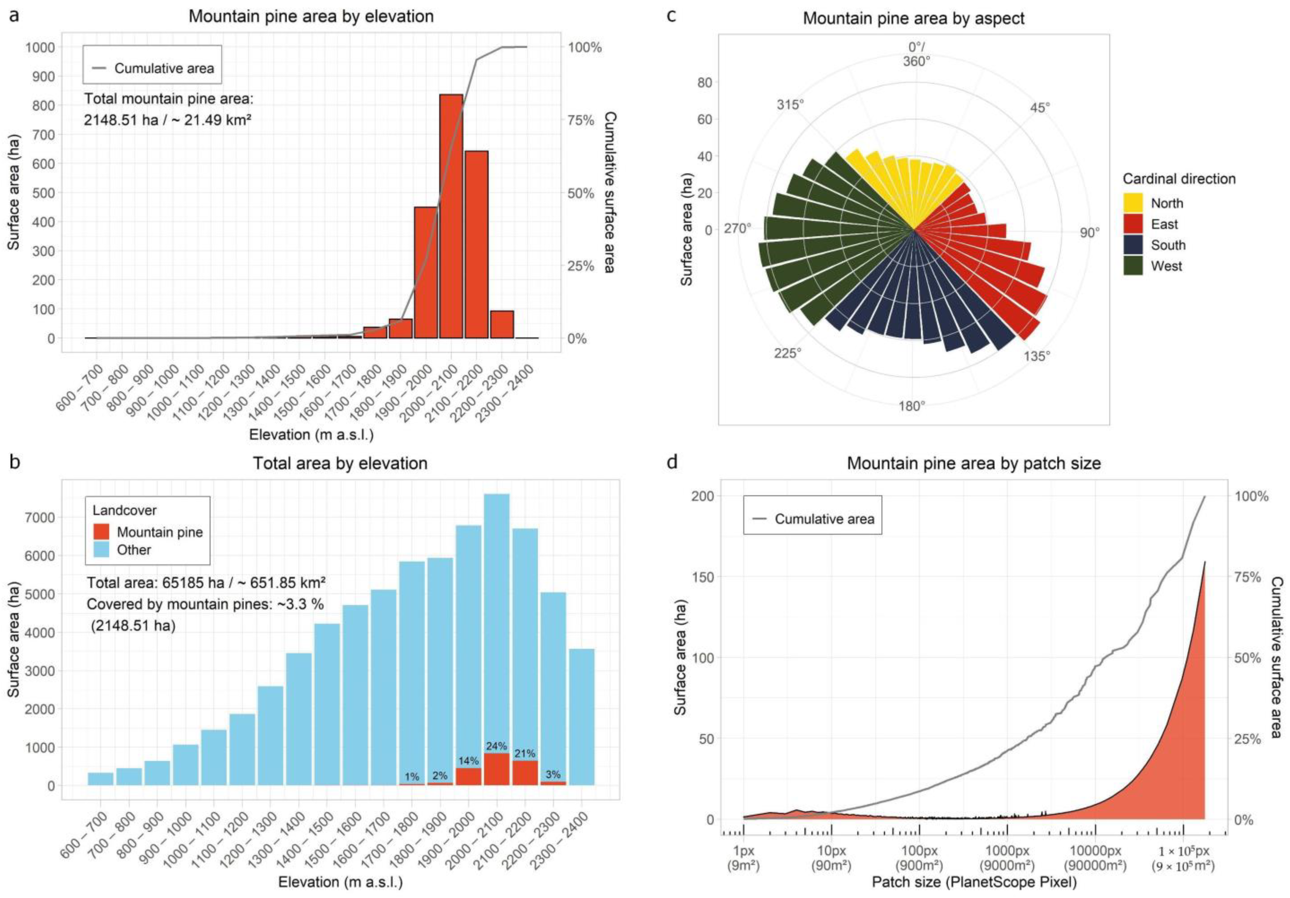
To create an accurate map of the overall coverage and spatial distribution of mountain pines in the Sarntal Alps,
(ii)
To quantify how the spatial resolutions of open-access Sentinel-2 (10 m) and commercial PlanetScope (3 m) data influence the mapping accuracy of mountain pines,
(iii)
To analyze which of the features previously used for alpine vegetation classification are the most useful for the delineation of mountain pines.
Our study will improve the overall understanding of how mountain pines can be accurately mapped using satellite observations by assessing the choice of satellite data and classification features. The derived mountain pine map for our study region is expected to support local forest management to monitor and assess recent and ongoing anthropogenic and climatic changes at the treeline.

2. Materials and Methods
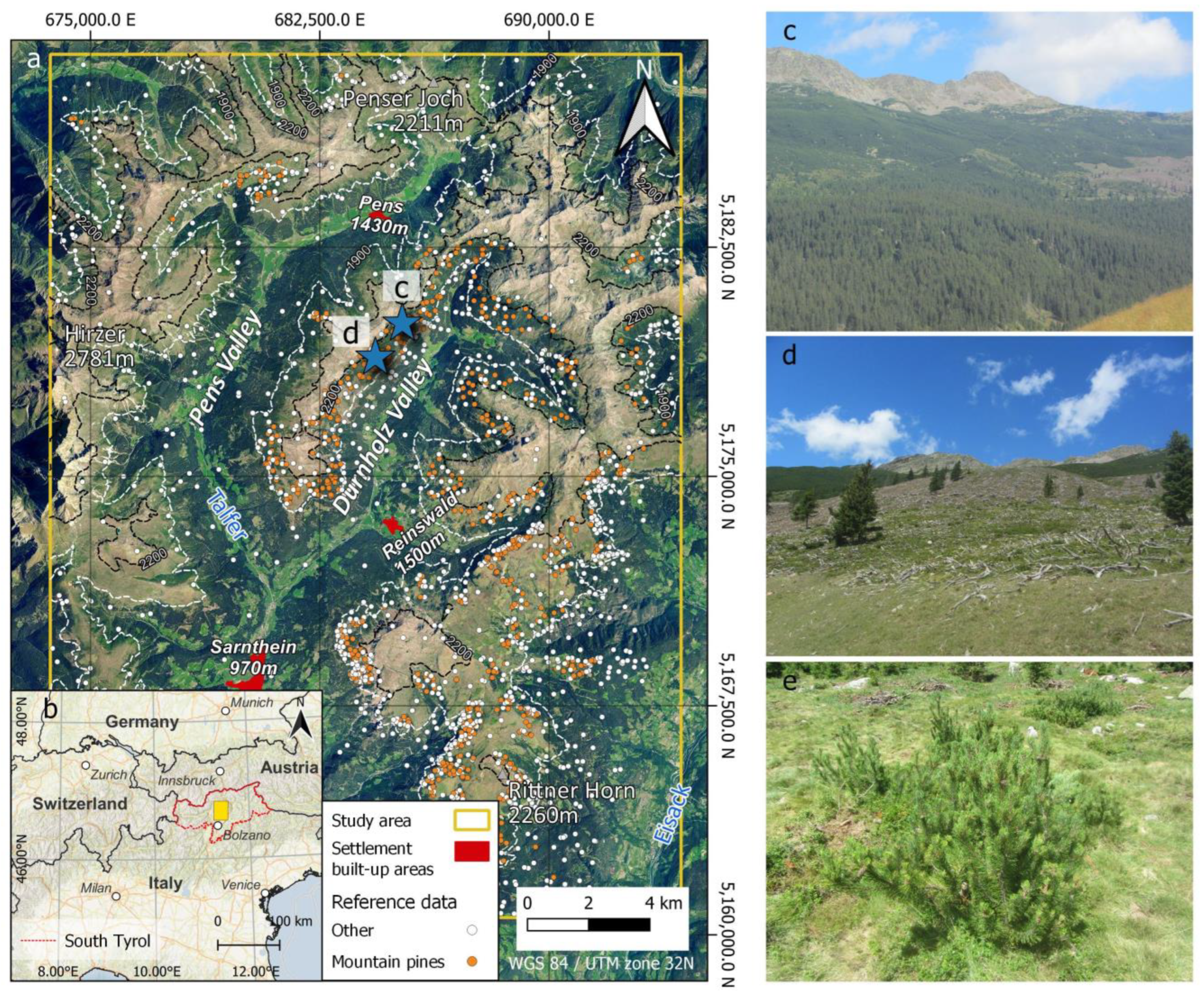
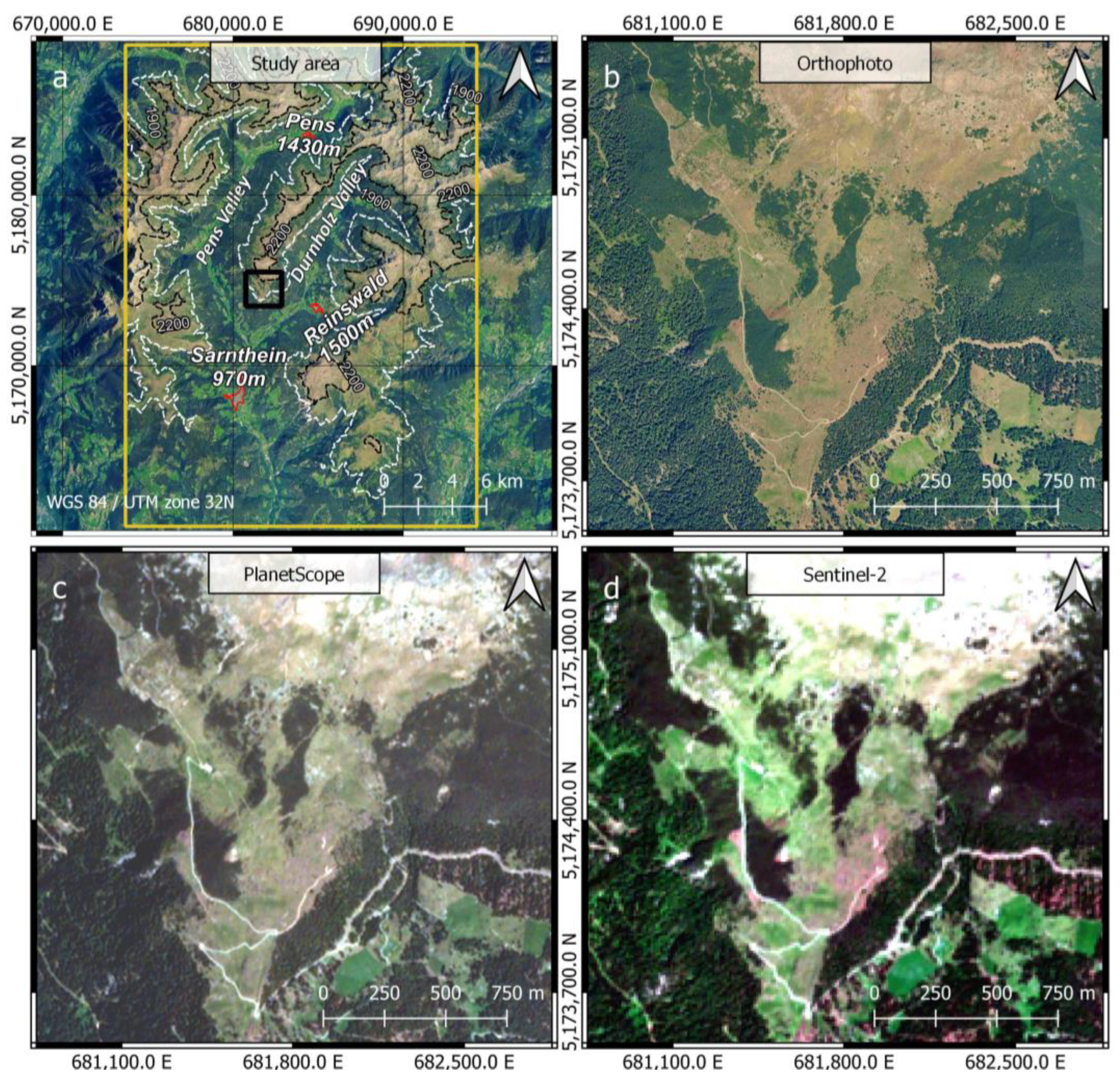
2.1. Study Area

The study area is located in South Tyrol, Northern Italy, and includes the subalpine and alpine altitudinal zones of the Sarntal Alps (Figure 1). It covers an area of 583 km2 and includes the entire Sarntal Valley with its side valleys (Pens Valley and Durnholz Valley). The orography of the Sarntal Alps is characterized by mostly gentle, moderately steep slopes, with elevations ranging from 923 m a.s.l. to 2781 m a.s.l. Due to the location at the southern edge of the Alps, the climate is characterized by moderate precipitation and a high number of sunny days [31]. At the valley floor (Sarnthein 970 m a.s.l.), the annual mean temperature is 8.4 C, while annual mean precipitation sums up to 908.7 mm/year [13]. With increasing altitude, annual mean temperature decreases to 1.1 C at 2260 m a.s.l. (Rittner Horn), and annual mean precipitation increases to 1016 mm/year [13].
The study area is dominated by conifers, which grow up to the treeline between 1800 and 2000 m a.s.l., while deciduous woods are rare [5]. While spruce-fire forests occur at the valley flood, subalpine spruce forests cover most slopes below the treeline. Mountain pines dominate the treeline, especially on the south-facing slopes of the Durnholz Valley and around the Rittner Horn, where they form large contiguous patches. Where mountain pines are less abundant, larch-pine forests characterize the treeline with the sporadic growing of green alder (Alnus virids). Overall, mountain pines occur in combination with green alder (Alnus viridis), spruce (Picea abies), larch (Larix decidua), swiss pine (Pinus cembra) and alpine dwarf shrubs (e.g., alpine rose (Rhododendron ferrugineum)) in our study area [5].
The use of mountain pine stands in the Sarntal Valley has intensified in the last years to serve the rising demand for wellness products in South Tyrol [32]. As a result, large contiguous mountain pine areas on the southeast-facing slopes of the Durnholz Valley have been clear-cut for the oil production by the three distilleries in the Sarntal Valley (Figure 1c,d).

2.2. Data

2.2.1. PlanetScope Imagery

We selected four cloud-free PlanetScope image datasets acquired in the snow-free summer months of 2020 (1 June 2020; 5 July 2020; 5 August 2020; 18 September 2020). PlanetScope is a satellite constellation consisting of over 150 CubeSats (Doves) flying in a near-polar orbit at 475 km altitude [33], which allows for observing the entire Earth’s land surface on a daily basis [34]. The constellation has been continuously recording data since 2016 and has been enlarged by additional Dove generations with enhanced sensor systems (1st generation: PS2, 2nd generation: PS2.SD and 3rd generation: PSB.SD). PlanetScope imagery is acquired at a spatial resolution of 3.7 m and three (Blue, wavelength λ = 455–515 nm; Green λ = 500–90 nm; Red λ = 590–70 nm) or four bands (additional near infrared (NIR) λ = 780–860 nm) depending on the generation [33].
For this study, we used the PlanetScope PS2 (Blue, Green, Red and NIR) orthorectified and atmospherically corrected “Analytic Ortho Scene” surface reflectance product (resampled to 3 m) [33]. Further pre-processing and analysis steps were performed using the open-source software R [35] and QGIS [36]. First, for each time step the individual scenes of each date were mosaicked by averaging the spectral information of overlapping areas. Second, remaining patches of snow and cloud covered areas (present in scenes acquired on 1 June 2020 and 18 September 2020) were masked using PlanetScope’s data product mask (UDM2) [33] and an additional threshold based on overall brightness [37,38]. We then filled these data gaps with the information from the closest observations in time.

2.2.2. Sentinel-2 Imagery

Complementary to PlanetScope, we obtained multi-temporal images from the Sentinel-2 Multispectral Instrument (MSI). The European Space Agency’s (ESA) Sentinel-2 mission consists of two identical satellites (Sentinel-2A & Sentinel-2B) with a repetition rate of 5 days. The MSI sensor has thirteen spectral bands in the wavelength range between blue (λ = 443 nm) and shortwave infrared (SWIR) (λ = 2190 nm) in three different geometric resolutions (10 m, 20 m, 60 m) [39].
We downloaded four cloud-free Sentinel-2 L2A (surface reflectance) images from the summer period of 2020 (2 June 2020; 7 July 2020; 26 August 2020; 5 September 2020) that were close in time to the acquisition dates of PlanetScope. For comparability, we selected only the bands (Blue, Green, Red and NIR) with a pixel size of 10 m. We cropped the Sentinel-2 images to the extent of the study area and masked snow and cloud cover using an overall brightness threshold of these four spectral bands. The resulting data gaps were then filled with the observations closest in time.

2.2.3. LiDAR Data Derivatives

We obtained a DTM at 2.5 m spatial resolution that was generated from airborne Light Detection and Ranging (LiDAR) data acquired in 2006 [40]. The DTM was resampled to the resolution of PlanetScope and Sentinel-2 using a bilinear resampling technique. Additionally, we used a canopy height model (CHM) (2.5 m) derived from the same LiDAR data, which we resampled to the two satellite sensor pixel sizes (3 m and 10 m).

2.2.4. Reference Dataset

Reference data in mountain environments are often limited and outdated since field surveys in these regions are expensive, time consuming and demanding [20]. For our study, reference data on mountain pines were derived by the photointerpretation of recent aerial images by local experts (foresters working in the Sarntal Valley) and provided by the Forest Service of the Autonomous Province of Bolzano. Overall, reference vector data included 31 polygons indicating mountain pine stands (23.19 ha) and 13 polygons indicating other vegetation classes at the treeline ecotone (e.g., Pinus cembra, Alnus viridis, Rhododendron ferrugineum) (7.06 ha). From these polygons, 562 points were randomly extracted with a minimum distance of 30 m, resulting in 310 points for mountain pine class (class 1) and 252 points for other land cover classes (class 0). To ensure that bare areas in between mountain pine patches were not sampled for the mountain pine class, we applied a threshold based on the Normalized Difference Vegetation Index (NDVI) of the PlanetScope scene from 5 August 2020 and selected only sample points with NDVI values >0.4. Sample points in forest boundary regions were visually verified using an RGB airborne orthophoto (20 cm) from summer 2020 [41]. To also include other land cover classes present in the study area (e.g., grassland, bare soil, rocks and coniferous forest) and to account for the spatial restriction of the foresters’ reference data to the northern part of the Sarntal Valley, additional reference data (1654 points: 556 points (class 1) and 1098 points (class 0)) were randomly set and manually labeled over the entire study area with respect to the minimum distance (30 m) using the 2020 orthophoto as a visual interpretation reference. Additionally, an orthophoto from 2006 was used to ensure that no reference points in recently cleared mountain pine areas were included in the reference data set, which could cause confusion due to the outdated CHM. In combination with the randomly extracted reference points, this resulted in a reference dataset with 2216 points (Figure 1): 866 points (class 1) and 1350 points (class 0). The reference dataset was then split into training and validation datasets with a ratio of 70:30.

2.3. Methods

Mountain pine stands have similar morphological and anatomical needle characteristics to other subalpine coniferous trees (e.g., Scots pine (Pinus sylvestris) and Swiss pine (Pinus cembra)) [3,21] which lead to similar spectral characteristics (Figure 2). As a result, the satellite-based mapping of mountain pines is challenging [6,23,28,29] as they cannot be differentiated from other coniferous tree species based on their spectral properties only [23,28]. Moreover, the spectral confusion between mountain pine areas and alpine grasslands or dwarf shrub species can also reduce the classification accuracy [8,20]. To increase the class separability of mountain pines, we first derived complementary features from satellite and LiDAR data (Section 2.3.1), which we combined in different feature spaces (Section 2.3.2) for the subsequent classification (Section 2.3.3).

2.3.1. Feature Extraction

We extracted multiple features to quantify and understand their added value for mapping mountain pines.
Vegetation indices such as the NDVI provide reliable information on the photosynthetic activity and health of plants [42], and additional NDVI layers can improve the tree species mapping in mountain environments [6,10,23,24]. Therefore, we calculated the NDVI for each PlanetScope and Sentinel-2 image.
Topographic features allow for identifying the species-specific distribution within an alpine environment [23,24] and can increase the discrimination of alpine species [6,9,28]. The direct linkage of alpine vegetation with the relief offers a unique opportunity for the mapping of mountain pine areas. Mountain pines are mainly distributed at the treeline, colonize slopes, which are too steep for upright growing tree species, and are influenced by the exposition [1,6]; e.g., north-facing slopes in the Sarntal Alps are scarcely populated by the pine species [5]. For this reason, we calculated the slope and aspect based on the DTM.
Mountain pines grow in dense patches and show a characteristic growth structure that is more homogenous compared to other subalpine conifers [2,20,24]. By including this textural information, the class separability between mountain pines and other coniferous tree species can be improved [10,25,28,43]. We calculated a gray level co-occurrence matrix (GLCM) by Haralick et al. [44] for every PlanetScope and Sentinel-2 image. The GLCM is a popular approach to derive textural features and was successfully applied to map alpine vegetation types [22,24,25,28]. The GLCM describes the relationship of the gray values of two or more neighboring pixels and combines this into a frequency matrix [43,45] that can be used to calculate secondary textural statistics [46]. We chose the respective NIR band to calculate the GLCM due to its sensitivity to vegetation type, density and general plant health, following recent studies [28,29,46]. For computational reasons and statistical validity, quantization levels were reduced to 5-bit [43]. The distance between pixels during the calculation of GLCM was kept constant at one. We used the average of the four main interpixel angles (0°, 45°, 90° and 135°) based on our assumption that mountain pine areas do not have a preferred texture orientation. The selection of the secondary statistical features has a significant impact on the classification [43,46]. The homogeneity is particularly useful to capture the characteristic dense and intertwined growing form of mountain pines [28]. Additionally, secondary statistical features detecting edges can be useful to delineate single mountain pine patches [46]. Five secondary statistics—homogeneity, contrast, entropy, spatial mean and spatial variance (for a detailed description see [45,46])—were derived from GLCM for every PlanetScope resp. Sentinel-2 image.
The GLCM window size plays a crucial role, as the secondary statistics are calculated depending on it [46,47]. To exploit the complete capabilities of textural analysis, the selection of GLCM window size should be performed with respect to the target size and sensor spatial resolution [43]. Too-small windows cannot recognize the patterns as a whole, and too-large windows can mix the patterns of several classes [43,46]. For this reason, we calculated the five secondary statistics with iteratively increasing GLCM window sizes (3 × 3, 5 × 5, 7 × 7, 9 × 9, 11 × 11, 13 × 13, 15 × 15, 17 × 17, 23 × 23, 29 × 29, 35 × 35, 43 × 43 and 51 × 51 pixels) for both PlanetScope and Sentinel-2 data. Starting from the minimum window size of 3 × 3 pixels, we increased the windows by the minimum step size of 2 pixels until reaching a window size of 17 × 17 pixels. After this size, we chose larger increasing steps to calculate the GLCM window sizes in order to minimize spatial autocorrelation and computation time. We stopped the calculation after a window size of 51 × 51 pixels since no further increase in overall accuracy was visible for either PlanetScope or Sentinel-2 data.

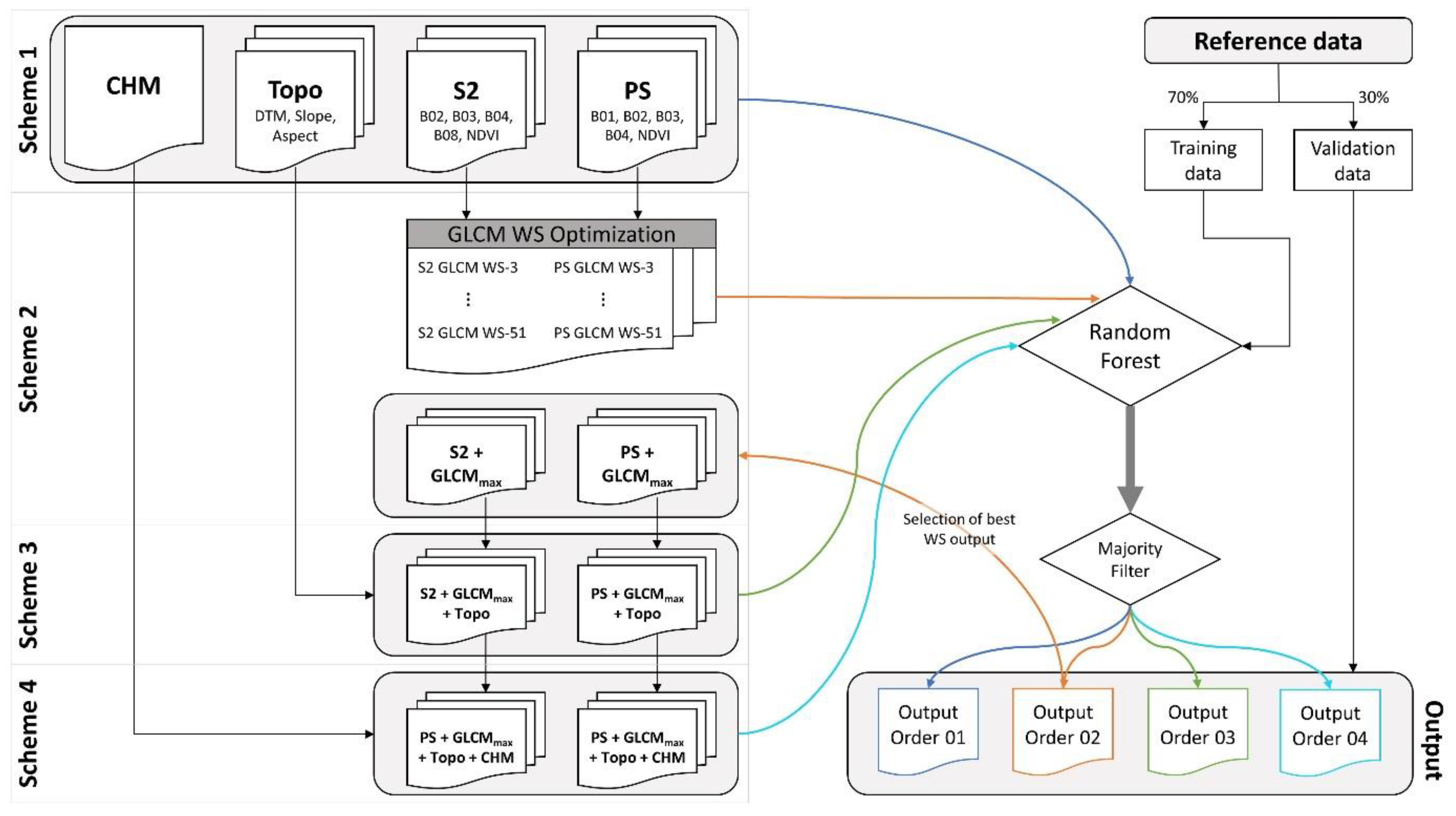
2.3.2. Feature Spaces and Classification Schemes

To assess the influence of the generated features and the spatial resolutions of PlanetScope and Sentinel-2, multiple feature spaces were created (Table 1) and tested in our classification workflow (Figure 3). The first feature space is a multi-temporal image stack of the four 4-band PlanetScope resp. Sentinel-2 images and the NDVI layer of each image (20 layers in total). The feature spaces were named PS and S2, respectively (Table 1). We used multi-temporal satellite imagery stacks because intra-annual changes in vegetation greenness can improve the classification of alpine vegetation [48] and especially of mountain pines [6,28]. Our third feature space (Topo) consisted of the LiDAR derived topographical features (elevation, slope and aspect) (Table 1). A valuable source for identifying alpine vegetation cover and species distribution is the CHM [27,49]. The characteristic growing height (<3 m) of mountain pines [1,2] can be used to differentiate the mountain pine from other conifers or dwarf shrubs at the treeline ecotone. Therefore, one feature space only includes the CHM. The four feature spaces (PS, S2, Topo and CHM) comprised classification scheme 1 and were classified individually.
Classification scheme 2 included the feature spaces PS + GLCMMAX and S2 + GLCMMAX. These feature spaces contain the multi-temporal imagery and NDVI stacks from classification scheme 1 combined with the five textural statistics for each image of the optimal GLCM window size. The optimal GLCM window size (GLCMMAX) was determined by iteratively classifying and validating each feature space and subsequently selecting the one with the highest overall accuracy (Figure 3).
Classification scheme 3 combines the feature spaces of scheme 2 (PS + GLCMMAX, S2 + GLCMMAX) with the Topo feature space. Classification scheme 4 joins the feature spaces from scheme 3 (PS + GLCMMAX + Topo, S2 + GLCMMAX + Topo) with the CHM feature space.

2.3.3. Random Forest Classification and Validation

We selected a Random Forest model [50] to map the mountain pine stands in the Sarntal Alps. Random Forest is a non-parametric machine learning algorithm that can handle high-dimensional datasets and was shown to be highly capable of accurately classifying alpine tree species [10,23,24,25,29]. For the individual feature spaces of each classification scheme (Table 1), we trained a Random Forest model with identical training data (Figure 3) using the R package “caret” [51]. The number of trees was kept constant at 500, as suggested in previous studies [23,24], and confirmed by our initial classification tests, which did not show a notable influence of the number of trees on the model output accuracies. To find the optimal number of features at each decision node for each feature space, we tuned the respective parameter using a 10-fold cross-validation approach. A majority filter (3 × 3) was then applied to each model output to reduce classification noise.
To assess the accuracy of the different mountain pine classifications, we compared the classification maps visually and derived the confusion matrix for each classification result using the validation dataset (Section 2.2.4). We calculated the overall accuracy (OA) (Equation (1)), Kappa coefficient, user’s accuracy (UA) (Equation (2)), and producer’s accuracy (PA) (Equation (3)) (Table A1, Table A2, Table A3, Table A4, Table A5, Table A6, Table A7, Table A8, Table A9 and Table A10):
Overall   accuracy   ( OA ) = N 00 + N 11 N
User s   accuracy   ( UA ) = N 11 N 10 + N 11
Producer s   Accuracy   ( PA ) = N 11 N 01 + N 11
with N equivalent to the total number of reference points and N00 and N11 the number of correctly classified reference points for the other land cover class (class 0) and mountain pine class (class 1). The formulae of UA and PA are displayed for class 1 with N10 equivalent to the number of reference points falsely not classified as mountain pine (false negative) and N01 the number of reference points falsely classified as mountain pine (false positive).
Additionally, receiver operating characteristic (ROC) curves and the respective area under the curve (AUC) [52] were calculated for each classification result. ROC visualizes the tradeoff between true positive and false positive rates, which helps to assess the actual predictive power of a model [52]. AUC is a measure for the area between a model’s ROC curve and the diagonal representing a random classification result. High AUC values indicate a high class separability of the model [52].
We selected the classification with the highest OA to map and analyze the spatial pattern of mountain pines in the Sarntal Alps. To reduce the effects of the topographic relief in mountainous regions [53], we calculated the real surface area using the software SAGA GIS Version 8 [54] using the function “Real Surface Area” and the slope derived from the DTM. Additionally, we derived spatial statistics considering elevation, slope, aspect and patch size to better understand the distribution of mountain pines in our final classification result.

3. Results

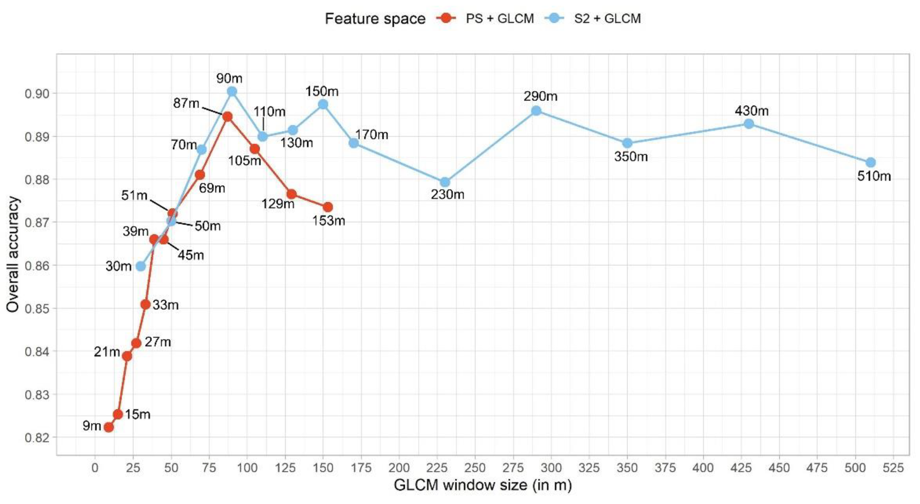
3.1. GLCM Window Size Optimization

The GLCM window size showed a noteable effect on the overall accuracy of the PS and S2 feature spaces (Figure 4). In general, overall accuracy increased at small GLCM window sizes for both satellite feature spaces. The effect of larger GLCM window sizes showed a stronger impact on overall accuracies of PS (0.82–0.89) than S2 (0.86–0.90) feature spaces. Thereby, S2 approaches the maximum OA at a GLCM window size of 9 pixels (90 m) and saturates afterwards. In comparison, the OA of PS rises until a GLCM window size of 29 pixels (87 m) and decreases then with increasing window sizes. Within this range, the GLCM secondary statistics can best describe the mountain pine stands in the study area and determine the optimal GLCM window sizes (GLCMMAX) for PS (29 × 29 pixels) and S2 (9 × 9 pixels).

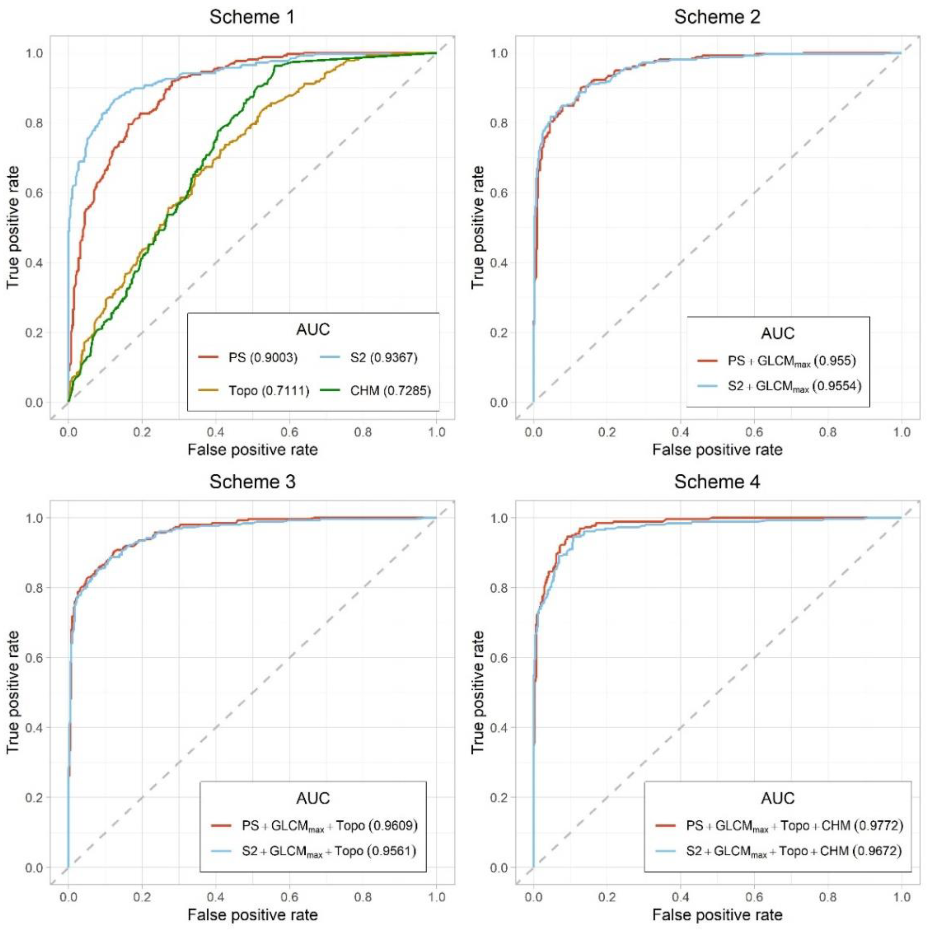
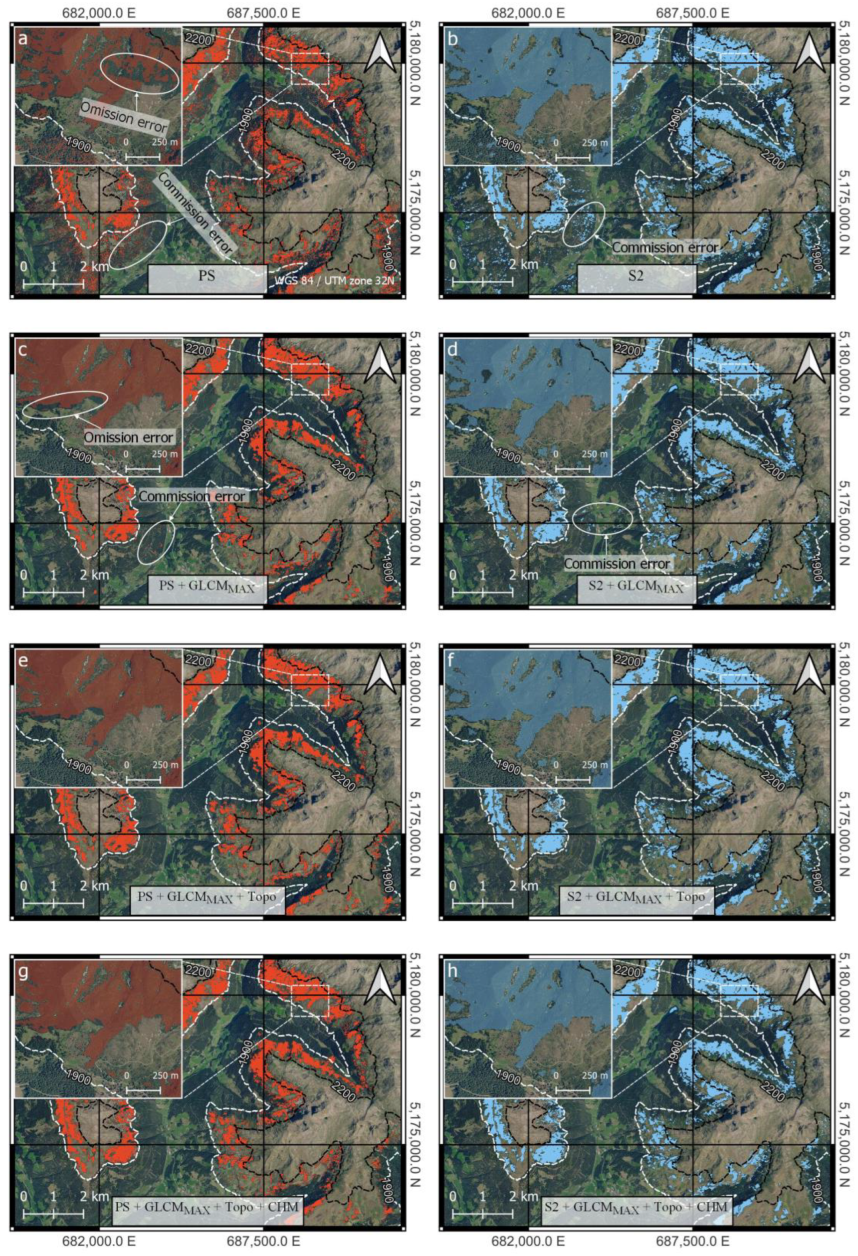
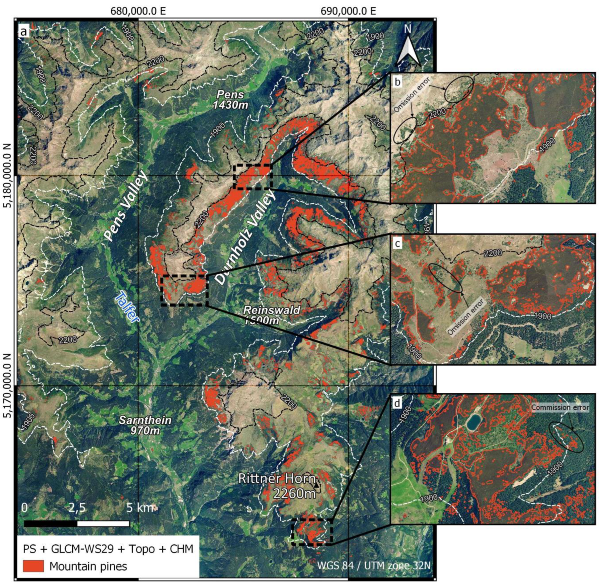
3.2. Classification Results

Classification accuracies of scheme 1 varied strongly among the different feature spaces and showed the overall lowest accuracy among all schemes (Figure 5, Table A1, Table A2, Table A3, Table A4, Table A5, Table A6, Table A7, Table A8, Table A9 and Table A10). LiDAR derived feature spaces resulted in overall accuracies of 65.0% (Topo) and 64.2 % (CHM), while the multi-temporal satellite feature spaces performed significantly better. Thereby, the overall accuracy of PS (81.2%) was lower than S2 (87.2%). For PS also, the PA (74.5%) and UA (76.6%) were considerably lower compared to the PA (80.9%) and UA (85.3%) of the S2 feature space. Particularly visible are false positive pixels (commission error) in the forest areas on the south-facing slopes of Durnholz Valley (Figure 6a), which are also visible in the results of the S2 feature space (Figure 6b). For PS, additional false negative pixels (omission error) occurred in some large, contiguous patches, where mountain pine was incorrectly not detected (Figure 6a). Mountain pine classifications of scheme 2 showed overall higher OAs than scheme 1 and a slightly higher accuracy for S2 + GLCMMAX (90.0%) than for PS + GLCMMAX (89.5%). The inclusion of GLCM textural features led to an increase in the PA and UA of PS + GLCMMAX (80.3% and 91.6%) and S2 + GLCMMAX (81.7% and 91.7%), which is also visible in the decrease of false positive pixels (Figure 6c,d). The addition of GLCMMAX also resulted in a reduction of the omitted mountain pine pixels in the PS + GLCMMAX feature space, while some boundary areas still experienced some confusion (Figure 6c). The OAs of mountain pine classifications did not change significantly when topographical features were added to the feature space scheme 3). However, our visual assessment showed that false positive pixels in the valley were almost completely eliminated (Figure 6e,f). The inclusion of CHM (scheme 4) slightly improved both classification results and led to the best results for PS + GLCMMAX + Topo + CHM (91.0%) and S2 + GLCMMAX + Topo + CHM (90.6%).
ROC and AUC values confirmed the accuracy assessments and our visual evaluation of the different mountain pine classifications (Figure 5 and Figure 6). For scheme 1, the performance of the S2 classification model based on ROC curves indicated a higher true positive rate compared to PS (Figure 7). However, PS performed much better in predicting true positive pixels than Topo or CHM. Likewise, the AUC of S2 (0.94) indicated that the class separability performance is significantly higher compared to the PS classification model (0.90). ROC curves and AUC values of classification scheme 2 confirmed a similar predictive power of both models, and AUC increased to 0.96 for both PS + GLCMMAX and S2 + GLCMMAX. For scheme 3, class separability for PS + GLCMMAX + Topo (0.96) and S2 + GLCMMAX + Topo remained constant (0.96). The ROC curves of classification scheme 4 showed a slightly better performance of PS + GLCMMAX + Topo + CHM compared to S2 + GLCMMAX + Topo + CHM, due to the lower number of false positive and the higher number of true positive pixels. Additionally, AUC indicated a minor improvement in class separability for both feature spaces (PS + GLCMMAX + Topo + CHM, AUC: 0.98; S2 + GLCMMAX + Topo + CHM, AUC: 0.97).
Figure 8 shows the spatial pattern of mountain pines in the entire study area classified by the PS + GLCMMAX + Topo + CHM feature space (OA 91%). Large areas of extensive and homogenous mountain pine patches were classified in the northern Sarntal Alps (Durnholz Valley) (Figure 8b,c). In general, mountain pine stands could be accurately delineated from the forest boundary (Figure 8b). However, smaller single patches of mountain pines at the border of large mountain pine stands were sometimes omitted (Figure 8b,c) while few mountain pines stands were wrongfully detected within the forest areas close to the timber line (Figure 8d). Around the Rittner Horn, mountain pines are more sparsely distributed but occur in large patches (Figure 8d). Our map suggests that mountain pines do not grow in the western mountain range of Sarntal Alps, except small parts in the northwestern part of the Pens Valley.
Based on our map, mountain pines cover 21.49 km2 of the Sarntal Alps (Figure 9), which accounts for 3.3% of the entire study area (Figure 9b). The largest mountain pine stands are found at altitudes between 2000–2100 m a.s.l. (Figure 9a), summing up to 24% (837 ha) of the total surface area at this elevation (Figure 9b). Overall, 90% (1929 ha) of all mountain pines in the Sarntal Alps grow at altitudes between 1900 and 2200 m a.s.l. (Figure 9a) and primarily occur on west- (29%) and south-facing (28%) slopes (Figure 9c). This pattern aligns with the large mountain pine areas on the west- and southeast-facing slopes in Durnholz Valley (Figure 8). At north- and east-facing slopes, mountain pine stands are less common, covering 20% and 23% of the total mountain pine surface area. The mountain pine in the Sarntal Alps tends to grow in large, contiguous patches (Figure 9d).
Although small patches are much more frequent, they cover only a small area. The 10,851 patches with a size smaller than 10 PlanetScope pixels (90 m2) only account for 2% (41 ha) of the mountain pine surface area. In comparison, the single largest patch (176,784 pixels; 159 ha) covers 8%, while the ten largest patches account for 37 % (726 ha) of the mountain pine area.

4. Discussion

The classification of mountain pines in an alpine environment was tested using optical satellite imagery with different spatial resolutions—PlanetScope (3 m) and Sentinel-2 (10 m)—and additional textural (GLCM), topographical (elevation, slope and aspect) and canopy height (CHM) features.

4.1. Influence of Spatial Resolution

In recent years, the usage of high-resolution satellite data for treeline ecotone mapping applications increased [55]. Especially in mountain regions with a complex treeline ecotone, a high spatial sensor resolution is needed to accurately map the different vegetation species [56,57]. We assumed that due to the higher resolution of PlanetScope, the mountain pine stands could be better delineated from conifers, especially in areas with strong intertwining between mountain pines and forested areas. However, our results indicate that Sentinel-2 behaves similarly to PlanetScope and even outperforms it by solely using the multitemporal image stacks (scheme 1). With the successive inclusion of textural and topographical features (schemes 2–4), the classification accuracy of PlanetScope and Sentinel-2 converges with only minimal differences in OA and AUC values. The best classification was achieved by the PlanetScope feature space (scheme 4) having the highest OA and AUC values. Yet, despite the marginally worse validation statistics, S2 + GLCMMAX + Topo + CHM still achieves excellent results in the delineation of mountain pine areas. A possible explanation for the similar behavior of PlanetScope and Sentinel-2 is the size distribution of the mountain pine fields. In the Sarntal Alps, mountain pine grows over large areas in contiguous patches. These can be accurately detected even with the lower resolution of Sentinel-2. Therefore, the good performance of Sentinel-2 also depends on the local specific growing forms of the mountain pines in the Sarntal Alps and may lead to worse results if the size distribution of the mountain pines changes (e.g., smaller, scattered patches). However, a good performance of Sentinel-2 was previously reported in other studies that classified mountain pine stands (e.g., PA 91.98%, UA 97.39% [10]; PA 85.3%, UA 93.9% [23]). The addition of the SWIR bands could further improve the classification results [26,48]. In contrast to other studies [56,57], it can be concluded that the higher spatial resolution does not necessarily lead to an improved classification of treeline species such as mountain pines. Further mapping approaches could therefore make use of the freely available Sentinel-2 imagery, which thus allows investigating larger study areas.

4.2. Feature Selection and Importance

The satisfactory results from feature spaces PS and S2 (scheme 1) are most likely due to their composition as multitemporal stacks, confirming several studies showing such effects (e.g., [10,23,48]). However, obtaining multiple useful optical acquisitions over a regional-scale mountainous area such as the Sarntal Alps (583 km2) is challenging due to short seasons, long snow cover presence and high cloud cover. Especially the high repetition rate of PlanetScope (majority of acquired images with revisit time <36 h) [34], allows to generate multitemporal image stacks in alpine environments. Temporal differences between the August (21 days) and September (13 days) scenes of PlanetScope and Sentinel-2 may capture differences in the phenological cycle of different species. Compared to other species (e.g., Larix decidua), the mountain pine remains constant in color and does not lose its needles. Therefore, the results of both feature spaces (PS and S2) should still be comparable.
The addition of the GLCM statistics (scheme 2), led to the greatest improvement of the OA for both PlanetSope (8.29%) and Sentinel-2 (2.87%). Texture features circumvent the challenging spectral discrimination between mountain pines and other subalpine conifers [23,28] by including the characteristic physiognomy of the mountain pine. While previous studies used GLCM features to map alpine vegetation species with a predefined window size without prior testing [22,24,25], our results suggest that an optimization process to identify the best GLCM window size (GLCMMAX) can improve the classification result significantly and should be implemented in future mapping approaches to account for study site characteristics and observed classes. In this study, mountain pine stands in the Sarntal Valley can be best captured with a window size ranging from 87 to 90 m–29 × 29 (PlanetScope) (7569 m2) and 9 × 9 (Sentinel-2) pixels (8100 m2).
Topographical features (scheme 3) eliminated misclassifications on the slopes of the Sarntal Valley (Figure 6), but changes in the OA are indistinct. Our results indicate that LiDAR-derived high-resolution topographic data (2.5 m) could be likely substituted by freely available lower resolution DEMs (e.g., Copernicus DEM (30 m) or SRTM DEM (30 m)) since the DEM does not lead to a more accurate detection of small-scale patches but, rather, incorporates large-scale elevation differences into the classification.
The CHM is a valuable feature for identifying mountain pines due to the distinct height difference to other coniferous trees [1,26,49] but only in combination with other information. When using just CHM as the input, confusion with objects of a similar height leads to a low OA (64.21%). The added value of CHM as an additional dataset is visible in classification scheme 4, where the best OA for both PlanetScope (90.96%) and Sentinel-2 (90.65%) was achieved. The temporal mismatch between the CHM and reference data might have had an influence on all classification results, including the CHM feature. However, we ensured that no reference points are located in areas affected by clearings between 2006 and 2020 by visually comparing orthophotos of these years. Our results indicate that with an adequate reference sampling technique and classification scheme, even an outdated CHM is useful for classifying mountain pines. Nevertheless, the findings indicate that using solely multitemporal spectral and textural information from four-band (blue, green, red, NIR) optical imagery already produces satisfactory results for mapping mountain pines in the study area—without considering auxiliary data sources (e.g., DTM or CHM). It should be noted that airborne LiDAR acquisitions are expensive and not available for large areas, which limits the transferability of an approach relying on the CHM. While we used LiDAR metrics only as an additional optional feature to test its added value, future research could also assess LiDAR metrics features of globally available missions (e.g., NASA´s Global Ecosystem Dynamics Investigation (GEDI) [58]) without computing textural features.

4.3. Classification Evaluation

The final classification accurately mapped mountain pine stands in the complex treeline ecotone. However, few misclassifications were apparent. Our classification underpredicted mountain pines slightly with a higher user´s accuracy (UA: 90.28%) than producer´s accuracy (PA: 86.1%), which aligns with the results of other studies [8,10,23,26]. Additionally, single conifers within mountain pine stands could not be detected due to the spatial resolution of the satellite imagery (Figure 8c). In some areas, confusion also occurred in areas where the regrowth of mountain pines was visible (Figure 8d). This was probably due to the low textural and spectral contrast between the small regrowing mountain pines and surrounding grasslands. Additionally, omitted mountain pine stands can be found in some edge areas around larger mountain pine patches (Figure 8b,c). One possible explanation could be that, due to the relatively large GLCMMAX window sizes, the textural signal of the smaller and more heterogeneous edge mountain pine stands were obliterated during the GLCM statistic calculation [43,46]. A smaller GLCM window size could reduce this error to some degree but would introduce misclassifications in other regions of the study area (e.g., at forest boundaries). To account for misclassifications at the boundary areas of mountain pine patches, an object-based approach implementing a region growing algorithm might produce beneficial results [26].
Besides, the further differentiation of subclasses within the “other land cover” class might increase the classification accuracy. However, high-quality, expert-based reference data were only available for the mountain pine class, and detailed knowledge about the land cover in the study area was not available. Hence, a binary classification model was chosen, which also reduces the amount of work required to sample reference data.
Current mapping methods used by local foresters have consisted of intensive field campaigns and time-consuming orthophoto interpretation so far. Therefore, our automated mapping process reduces the required resources for mapping mountain pines tremendously and fosters a continued monitoring of the mountain pine areas. In the future, our approach will be used to map mountain pine stands in the Sarntal Alps over time to support the local forest authorities in assuring their sustainable use. Recent logging activities, for instance, could be detected by comparing maps in time and PlanetScope or Sentinel-2 date back to 2016 and 2015. For the mapping of mountain pine stands of the more distant past, other comparable optical satellite imagery (e.g., RapidEye [28], Landsat 5–8 [6]) or multispectral orthophotos [22,25] could be used. Additionally, long-term monitoring could also inform of the climate-induced expansion of mountain pines towards the alpine altitudinal zone [7,12,15]. Furthermore, this methodology could possibly be transferred to other alpine regions if sufficient reference data are available.

5. Conclusions

This study used multitemporal PlanetScope (3 m) and Sentinel-2 (10 m) imagery in combination with NDVI to map mountain pine (P. mugo) stands in the Sarntal Alps, South Tyrol. By successively adding additional features (textural features (GLCM), topographic features (elevation, slope and aspect) and canopy height model (CHM)), the overall classification accuracy of mountain pines improved. Thereby, the largest accuracy increase was obtained by including textural information based on an optimal GLCM window size for PlanetScope (29 × 29 pixels (87 × 87 m)) and Sentinel-2 (9 × 9 pixels (90 × 90 m)). The inclusion of LiDAR-derived high-resolution auxiliary datasets, such as topographical data and canopy height, only marginally improved the classification result. Since textural features directly derived from the satellite imagery already produce sufficient mapping results, there is no pressing need for the implementation of costly auxiliary datasets (e.g., Lidar derived DTM or CHM). This results in the easy transferability of our methodology to other study regions if sufficient reference data are available. The best classification was obtained when combining PlanetScope with the GLCM statistics, topographical features and canopy height model. However, comparable results were achieved with Sentinel-2 data instead of PlanetScope, indicating that the spatial resolution has no major influence on the mapping accuracy of mountain pines in our study area. Because of the free availability of Sentinel-2 data, this classification approach is particularly well-suited for further mapping of mountain pine stands in other alpine regions.
The final mountain pine map will support local forest management by reducing the required resources to map P. mugo stands. This allows for more comprehensive monitoring and provides the basis for understanding changes due to the mountain pine usage and climatic changes at the treeline ecotone. Therefore, further research should implement the presented classification approach to map the annual extent of mountain pines in future years.

Author Contributions

Conceptualization, M.R., R.S., S.B. and T.U.; Formal analysis, M.R.; Methodology, M.R., R.S., S.B. and T.U.; Resources, M.R. and R.S.; Software, M.R.; Supervision, R.S., S.B. and T.U.; Validation, M.R.; Visualization, M.R.; Writing—original draft, M.R.; Writing—review and editing, M.R., R.S., S.B. and T.U. All authors have read and agreed to the published version of the manuscript.

Funding

This publication was supported by the Open Access Publication Fund of the University of Wuerzburg and the Department of Innovation, Research and University of the Autonomous Province of Bozen/Bolzano. No further external funding was received.

Data Availability Statement

The PlanetScope imagery used in this work was provided by Planet Labs through DLR’s RESA program (RESA-RESA, BMWi grant 50 EE 1612). The datasets generated during the study are available from the corresponding author on reasonable request.

Acknowledgments

We kindly thank Martin Stecher (Office for Forest Planning, Autonomous Province of Bolzano), Dieter Senn and Dominik Trenkwalder (Forestry station Sarntal, Autonomous Province of Bolzano) for providing the reference data, sharing their local knowledge, and expertise and organization of the field trip. The authors thank the Department of Innovation, Research and University of the Autonomous Province of Bozen/Bolzano for covering the Open Access publication costs.

Conflicts of Interest

The authors declare no conflict of interest.

Appendix A. Confusion Matrices and Accuracy Statistics for Classification Schemes

Table A1. PS classification (“scheme 1”).
Reference
Classification Class 0Class 1Total
Class 034666412
Class 159193252
Total405259664
Overall Accuracy and Kappa coefficient
OAKappa
0.81170.6024
Class Statistics
PAUA
Class 00.85430.8398
Class 10.74520.7659
Class 1 represents mountain pines. Class 0 represents other land cover types. OA = overall accuracy; PA = producer’s accuracy; UA = user’s accuracy; Kappa = Kappa coefficient.
Table A2. S2 classification (“scheme 1”).
Reference
Classification Class 0Class 1Total
Class 037049419
Class 136208244
Total406257663
Overall Accuracy and Kappa coefficient
OAKappa
0.87180.7274
Class Statistics
PAUA
Class 00.91130.8831
Class 10.80930.8525
Class 1 represents mountain pines. Class 0 represents other land cover types. OA = overall accuracy; PA = producer´s accuracy; UA = user´s accuracy; Kappa = Kappa coefficient.
Table A3. Topo classification (“scheme 1”).
Reference
Classification Class 0Class 1Total
Class 0302140442
Class 193130223
Total395270665
Overall Accuracy and Kappa coefficient
OAKappa
0.64960.253
Class Statistics
PAUA
Class 00.76460.6833
Class 10.48150.5830
Class 1 represents mountain pines. Class 0 represents other land cover types. OA = overall accuracy; PA = producer´s accuracy; UA = user´s accuracy; Kappa = Kappa coefficient.
Table A4. CHM classification (“scheme 1”).
Reference
Classification Class 0Class 1Total
Class 0280123403
Class 1115147262
Total395270665
Overall Accuracy and Kappa coefficient
OAOAKappa
0.64210.64210,2545
Class Statistics
PAUA
Class 00.70890.6948
Class 10.54440.5611
Class 1 represents mountain pines. Class 0 represents other land cover types. OA = overall accuracy; PA = producer´s accuracy; UA = user´s accuracy; Kappa = Kappa coefficient.
Table A5. PS + GLCMMAX (window size 29×29 pixels (87×87 m)) classification (“scheme 2”).
Reference
Classification Class 0Class 1Total
Class 038651437
Class 119208227
Total405259664
Overall Accuracy and Kappa coefficient
OAKappa
0.89460.7734
Class Statistics
PAUA
Class 00.95310.8833
Class 10.80310.9163
Class 1 represents mountain pines. Class 0 represents other land cover types. OA = overall accuracy; PA = producer´s accuracy; UA = user´s accuracy; Kappa = Kappa coefficient.
Table A6. S2 + GLCMMAX (window size 9 × 9 pixels (90 × 90 m)) classification (“scheme 2”).
Reference
Classification Class 0Class 1Total
Class 038747434
Class 119210229
Total406257663
Overall Accuracy and Kappa coefficient
OAKappa
0.90050.786
Class Statistics
PAUA
Class 00.95320.8917
Class 10.81710.9170
Class 1 represents mountain pines. Class 0 represents other land cover types. OA = overall accuracy; PA = producer´s accuracy; UA = user´s accuracy; Kappa = Kappa coefficient.
Table A7. PS + GLCMMAX + Topo classification (“scheme 3”).
Reference
Classification Class 0Class 1Total
Class 039559454
Class 110200210
Total405259664
Overall Accuracy and Kappa coefficient
OAKappa
0.89610.7739
Class Statistics
PAUA
Class 00.97530.8700
Class 10.77220.9524
Class 1 represents mountain pines. Class 0 represents other land cover types. OA = overall accuracy; PA = producer´s accuracy; UA = user´s accuracy; Kappa = Kappa coefficient.
Table A8. S2 + GLCMMAX + Topo classification (“scheme 3”).
Reference
Classification Class 0Class 1Total
Class 038551436
Class 121206227
Total406257663
Overall Accuracy and Kappa coefficient
OAKappa
0.89140.7662
Class Statistics
PAUA
Class 00.94830.8830
Class 10.80160.9075
Class 1 represents mountain pines. Class 0 represents other land cover types. OA = overall accuracy; PA = producer´s accuracy; UA = user´s accuracy; Kappa = Kappa coefficient.
Table A9. PS + GLCMMAX + Topo + CHM classification (“scheme 4”).
Reference
Classification Class 0Class 1Total
Class 038136417
Class 124223247
Total405259664
Overall Accuracy and Kappa coefficient
OAKappa
0.90960.8085
Class Statistics
PAUA
Class 00.94070.9137
Class 10.86100.9028
Class 1 represents mountain pines. Class 0 represents other land cover types. OA = overall accuracy; PA = producer´s accuracy; UA = user´s accuracy; Kappa = Kappa coefficient.
Table A10. S2 + GLCMMAX + Topo + CHM classification (“scheme 4”).
Reference
Classification Class 0Class 1Total
Class 038238420
Class 124219243
Total406257663
Overall Accuracy and Kappa coefficient
OAKappa
0.90650.801
Class Statistics
PAUA
Class 00.94090.9095
Class 10.85210.9012
Class 1 represents mountain pines. Class 0 represents other land cover types. OA = overall accuracy; PA = producer´s accuracy; UA = user´s accuracy; Kappa = Kappa coefficient.

References

  1. Leuschner, C.; Ellenberg, H. Ecology of Central European Forests: Vegetation Ecology of Central Europe, Volume I; Springer: Cham, Switzerland, 2017; ISBN 9783319430423. [Google Scholar]
  2. Holtmeier, F.-K. What Does the Term “Krummholz” Really Mean? Observations with Special Reference to the Alps and the Colorado Front Range. Mt. Res. Dev. 1981, 1, 253. [Google Scholar] [CrossRef]
  3. Boratyńska, K.; Jasińska, A.K.; Boratyński, A. Taxonomic and geographic differentiation of Pinus mugo complex on the needle characteristics. Syst. Biodivers. 2015, 13, 581–595. [Google Scholar] [CrossRef]
  4. Stiegler, J.; Binder, F. Grünerle oder Latsche?—Eine Frage des Standorts. In LWF Aktuell 108: Energieholz Nutzen-Nährstoffe Bewahren; Schmidt, O., Zahner, V., Eds.; Bayrische Landesanstalt für Wald und Forstwirtschaft: Freising, Germany, 2016; pp. 54–57. [Google Scholar]
  5. Autonome Provinz Bozen. Waldtypisierung Südtirol Band 2: Waldgruppen, Naturräume, Glossar; 2010. Available online: https://www.provincia.bz.it/land-forstwirtschaft/wald-holz-almen/interaktive-karte.asp?publ_action=300&publ_image_id=197931 (accessed on 29 June 2022).
  6. Roșca, S.; Șimonca, V.; Bilașco, Ș.; Vescan, I.; Fodorean, I.; Petrea, D. The Assessment of Favourability and Spatio-Temporal Dynamics of Pinus Mugo in the Romanian Carpathians Using GIS Technology and Landsat Images. Sustainability 2019, 11, 3678. [Google Scholar] [CrossRef] [Green Version]
  7. Dai, L.; Palombo, C.; van Gils, H.; Rossiter, D.G.; Tognetti, R.; Luo, G. Pinus mugo Krummholz Dynamics During Concomitant Change in Pastoralism and Climate in the Central Apennines. Mt. Res. Dev. 2017, 37, 75–86. [Google Scholar] [CrossRef]
  8. Rujoiu-Mare, M.-R.; Olariu, B.; Mihai, B.-A.; Nistor, C.; Săvulescu, I. Land cover classification in Romanian Carpathians and Subcarpathians using multi-date Sentinel-2 remote sensing imagery. Eur. J. Remote Sens. 2017, 50, 496–508. [Google Scholar] [CrossRef] [Green Version]
  9. Švajda, J.; Solár, J.; Janiga, M.; Buliak, M. Dwarf Pine (Pinus mugo) and Selected Abiotic Habitat Conditions in the Western Tatra Mountains. Mt. Res. Dev. 2011, 31, 220–228. [Google Scholar] [CrossRef]
  10. Kovačević, J.; Cvijetinović, Ž.; Lakušić, D.; Kuzmanović, N.; Šinžar-Sekulić, J.; Mitrović, M.; Stančić, N.; Brodić, N.; Mihajlović, D. Spatio-Temporal Classification Framework for Mapping Woody Vegetation from Multi-Temporal Sentinel-2 Imagery. Remote Sens. 2020, 12, 2845. [Google Scholar] [CrossRef]
  11. Calabrese, V.; Carranza, M.; Evangelista, A.; Marchetti, M.; Stinca, A.; Stanisci, A. Long-Term Changes in the Composition, Ecology, and Structure of Pinus mugo Scrubs in the Apennines (Italy). Diversity 2018, 10, 70. [Google Scholar] [CrossRef] [Green Version]
  12. Lukasová, V.; Bucha, T.; Mareková, Ľ.; Buchholcerová, A.; Bičárová, S. Changes in the Greenness of Mountain Pine (Pinus mugo Turra) in the Subalpine Zone Related to the Winter Climate. Remote Sens. 2021, 13, 1788. [Google Scholar] [CrossRef]
  13. Crespi, A.; Matiu, M.; Bertoldi, G.; Petitta, M.; Zebisch, M. A high-resolution gridded dataset of daily temperature and precipitation records (1980–2018) for Trentino-South Tyrol (north-eastern Italian Alps). Earth Syst. Sci. Data 2021, 13, 2801–2818. [Google Scholar] [CrossRef]
  14. Gottfried, M.; Pauli, H.; Futschik, A.; Akhalkatsi, M.; Barančok, P.; Benito Alonso, J.L.; Coldea, G.; Dick, J.; Erschbamer, B.; Fernández Calzado, M.R.; et al. Continent-wide response of mountain vegetation to climate change. Nat. Clim. Chang. 2012, 2, 111–115. [Google Scholar] [CrossRef]
  15. Dirnböck, T.; Dullinger, S.; Grabherr, G. A regional impact assessment of climate and land-use change on alpine vegetation. J. Biogeogr. 2003, 30, 401–417. [Google Scholar] [CrossRef]
  16. Ballian, D.; Ravazzi, C.; de Rigo, D.; Caudullo, G. Pinus mugo in Europe: Distribution, habitat, usage and threats. In European Atlas of Forest Tree Species, 2016th ed.; San-Miguel-Ayanz, J., de Rigo, D., Caudullo, G., Durrant, T.H., Mauri, A., Eds.; Publication Office of the European Union: Luxembourg, 2016; pp. 124–125. ISBN 9789279367403. [Google Scholar]
  17. Petelka, J.; Plagg, B.; Säumel, I.; Zerbe, S. Traditional medicinal plants in South Tyrol (northern Italy, southern Alps): Biodiversity and use. J. Ethnobiol. Ethnomed. 2020, 16, 74. [Google Scholar] [CrossRef] [PubMed]
  18. Rosenvald, R.; Lõhmus, A. For what, when, and where is green-tree retention better than clear-cutting? A review of the biodiversity aspects. For. Ecol. Manag. 2008, 255, 1–15. [Google Scholar] [CrossRef]
  19. Bowd, E.J.; Banks, S.C.; Strong, C.L.; Lindenmayer, D.B. Long-term impacts of wildfire and logging on forest soils. Nat. Geosci. 2019, 12, 113–118. [Google Scholar] [CrossRef]
  20. Wakulińska, M.; Marcinkowska-Ochtyra, A. Multi-Temporal Sentinel-2 Data in Classification of Mountain Vegetation. Remote Sens. 2020, 12, 2696. [Google Scholar] [CrossRef]
  21. Mosca, E.; Gugerli, F.; Eckert, A.J.; Neale, D.B. Signatures of natural selection on Pinus cembra and P. mugo along elevational gradients in the Alps. Tree Genet. Genomes 2016, 12, 9. [Google Scholar] [CrossRef]
  22. Král, K. Classification of Current Vegetation Cover and Alpine Treeline Ecotone in the Praděd Reserve (Czech Republic), Using Remote Sensing. Mt. Res. Dev. 2009, 29, 177–183. [Google Scholar] [CrossRef]
  23. Kollert, A.; Bremer, M.; Löw, M.; Rutzinger, M. Exploring the potential of land surface phenology and seasonal cloud free composites of one year of Sentinel-2 imagery for tree species mapping in a mountainous region. Int. J. Appl. Earth Obs. Geoinf. 2021, 94, 102208. [Google Scholar] [CrossRef]
  24. Spracklen, B.D.; Spracklen, D.V. Identifying European Old-Growth Forests using Remote Sensing: A Study in the Ukrainian Carpathians. Forests 2019, 10, 127. [Google Scholar] [CrossRef] [Green Version]
  25. Toscani, P.; Immitzer, M.; Atzberger, C. Texturanalyse mittels diskreter Wavelet Transformation für die objektbasierte Klassifikation von Orthophotos. Photogramm. Fernerkund. Geoinf. 2013, 2, 105–121. [Google Scholar] [CrossRef]
  26. Rüetschi, M.; Weber, D.; Koch, T.L.; Waser, L.T.; Small, D.; Ginzler, C. Countrywide mapping of shrub forest using multi-sensor data and bias correction techniques. Int. J. Appl. Earth Obs. Geoinf. 2021, 105, 102613. [Google Scholar] [CrossRef]
  27. Reese, H.; Nyström, M.; Nordkvist, K.; Olsson, H. Combining airborne laser scanning data and optical satellite data for classification of alpine vegetation. Int. J. Appl. Earth Obs. Geoinf. 2014, 27, 81–90. [Google Scholar] [CrossRef]
  28. Polychronaki, A.; Spindler, N.; Schmidt, A.; Stoinschek, B.; Zebisch, M.; Renner, K.; Sonnenschein, R.; Notarnicola, C. Integrating RapidEye and ancillary data to map alpine habitats in South Tyrol, Italy. Int. J. Appl. Earth Obs. Geoinf. 2015, 37, 65–71. [Google Scholar] [CrossRef]
  29. Dalponte, M.; Bruzzone, L.; Gianelle, D. Tree species classification in the Southern Alps based on the fusion of very high geometrical resolution multispectral/hyperspectral images and LiDAR data. Remote Sens. Environ. 2012, 123, 258–270. [Google Scholar] [CrossRef]
  30. Vaglio Laurin, G.; Del Frate, F.; Pasolli, L.; Notarnicola, C.; Guerriero, L.; Valentini, R. Discrimination of vegetation types in alpine sites with ALOS PALSAR-, RADARSAT-2-, and lidar-derived information. Int. J. Remote Sens. 2013, 34, 6898–6913. [Google Scholar] [CrossRef]
  31. Wilhalm, T. Floristic Biodiversity in South Tyrol (Alto Adige). In Climate Gradients and Biodiversity in Mountains of Italy; Pedrotti, F., Ed.; Springer International Publishing: Cham, Switzerland, 2018; pp. 1–17. ISBN 9783319679679. [Google Scholar]
  32. Osti, L.; Goffi, G. Lifestyle of health & sustainability: The hospitality sector’s response to a new market segment. J. Hosp. Tour. Manag. 2021, 46, 360–363. [Google Scholar] [CrossRef]
  33. Planet Labs. PlanetScope Product Specifications. Available online: https://assets.planet.com/docs/Planet_PSScene_Imagery_Product_Spec_June_2021.pdf (accessed on 8 July 2021).
  34. Roy, D.P.; Huang, H.; Houborg, R.; Martins, V.S. A global analysis of the temporal availability of PlanetScope high spatial resolution multi-spectral imagery. Remote Sens. Environ. 2021, 264, 112586. [Google Scholar] [CrossRef]
  35. R Core Team. R: A Language and Environment for Statistical Computing; R Foundation for Statistical Computing: Wien, Austria, 2021. [Google Scholar]
  36. QGIS Development Team. QGIS Geographic Information System; Open Source Geospatial Foundation: Beaverton, OR, USA, 2021. [Google Scholar]
  37. Crane, R.G.; Anderson, M.R. Satellite discrimination of snow/cloud surfaces. Int. J. Remote Sens. 1984, 5, 213–223. [Google Scholar] [CrossRef]
  38. Dozier, J. Spectral signature of alpine snow cover from the landsat thematic mapper. Remote Sens. Environ. 1989, 28, 9–22. [Google Scholar] [CrossRef]
  39. European Space Agency. Sentinel-2 User Handbook. Available online: https://sentinel.esa.int/documents/247904/0/Sentinel-2_User_Handbook/8869acdf-fd84-43ec-ae8c-3e80a436a16c (accessed on 20 July 2021).
  40. Autonome Provinz Bozen. Digitales Geländemodell DTM (2.5 × 2.5m). Available online: http://daten.buergernetz.bz.it/de/dataset/modello-digitale-del-terreno-dtm-25m (accessed on 14 January 2022).
  41. Autonome Provinz Bozen. Orthofoto 2020. Available online: http://daten.buergernetz.bz.it/de/dataset/ortofoto-2020 (accessed on 14 January 2022).
  42. Tucker, C.J.; Sellers, P.J. Satellite remote sensing of primary production. Int. J. Remote Sens. 1986, 7, 1395–1416. [Google Scholar] [CrossRef]
  43. Marceau, D.J.; Howarth, P.J.; Dubois, J.M.; Gratton, D.J. Evaluation Of The Grey-level Co-occurrence Matrix Method For Land-cover Classification Using Spot Imagery. IEEE Trans. Geosci. Remote Sens. 1990, 28, 513–519. [Google Scholar] [CrossRef]
  44. Haralick, R.M.; Shanmugam, K.; Dinstein, I. Textural Features for Image Classification. IEEE Trans. Syst. Man Cybern. 1973, SMC-3, 610–621. [Google Scholar] [CrossRef] [Green Version]
  45. Gebejes, A.; Huertas, R. Texture characterization based on grey-level co-occurrence matrix. Proc. Conf. Inform. Manag. Sci. 2013, 2, 375–378. [Google Scholar]
  46. Hall-Beyer, M. Practical guidelines for choosing GLCM textures to use in landscape classification tasks over a range of moderate spatial scales. Int. J. Remote Sens. 2017, 38, 1312–1338. [Google Scholar] [CrossRef]
  47. Zhou, J.; Yan Guo, R.; Sun, M.; Di, T.T.; Wang, S.; Zhai, J.; Zhao, Z. The Effects of GLCM parameters on LAI estimation using texture values from Quickbird Satellite Imagery. Sci. Rep. 2017, 7, 7366. [Google Scholar] [CrossRef] [PubMed]
  48. Immitzer, M.; Neuwirth, M.; Böck, S.; Brenner, H.; Vuolo, F.; Atzberger, C. Optimal Input Features for Tree Species Classification in Central Europe Based on Multi-Temporal Sentinel-2 Data. Remote Sens. 2019, 11, 2599. [Google Scholar] [CrossRef] [Green Version]
  49. Torresani, M.; Rocchini, D.; Sonnenschein, R.; Zebisch, M.; Hauffe, H.C.; Heym, M.; Pretzsch, H.; Tonon, G. Height variation hypothesis: A new approach for estimating forest species diversity with CHM LiDAR data. Ecol. Indic. 2020, 117, 106520. [Google Scholar] [CrossRef]
  50. Breiman, L. Random Forests. Mach. Learn. 2001, 45, 5–32. [Google Scholar] [CrossRef] [Green Version]
  51. Kuhn, M. Building Predictive Models in R Using the caret Package. J. Stat. Softw. 2008, 28, 1–26. [Google Scholar] [CrossRef] [Green Version]
  52. Fawcett, T. An introduction to ROC analysis. Pattern Recognit. Lett. 2006, 27, 861–874. [Google Scholar] [CrossRef]
  53. Hoechstetter, S.; Walz, U.; Le Dang, H.; Thinh, N.X. Effects of topography and surface roughness in analyses of landscape structure—A proposal to modify the existing set of landscape metrics. Landsc. Online 2008, 3, 1–14. [Google Scholar] [CrossRef]
  54. Conrad, O.; Bechtel, B.; Bock, M.; Dietrich, H.; Fischer, E.; Gerlitz, L.; Wehberg, J.; Wichmann, V.; Böhner, J. System for Automated Geoscientific Analyses (SAGA) v. 2.1.4. Geosci. Model Dev. 2015, 8, 1991–2007. [Google Scholar] [CrossRef] [Green Version]
  55. Chhetri, P.K.; Thai, E. Remote sensing and geographic information systems techniques in studies on treeline ecotone dynamics. J. For. Res. 2019, 30, 1543–1553. [Google Scholar] [CrossRef]
  56. Hill, R.; Granica, K.; Smith, G.; Schardt, M. Representation of an alpine treeline ecotone in SPOT 5 HRG data. Remote Sens. Environ. 2007, 110, 458–467. [Google Scholar] [CrossRef]
  57. Luo, G.; Dai, L. Detection of alpine tree line change with high spatial resolution remotely sensed data. J. Appl. Remote Sens 2013, 7, 73520. [Google Scholar] [CrossRef]
  58. Dubayah, R.; Blair, J.B.; Goetz, S.; Fatoyinbo, L.; Hansen, M.; Healey, S.; Hofton, M.; Hurtt, G.; Kellner, J.; Luthcke, S.; et al. The Global Ecosystem Dynamics Investigation: High-resolution laser ranging of the Earth’s forests and topography. Sci. Remote Sens. 2020, 1, 100002. [Google Scholar] [CrossRef]
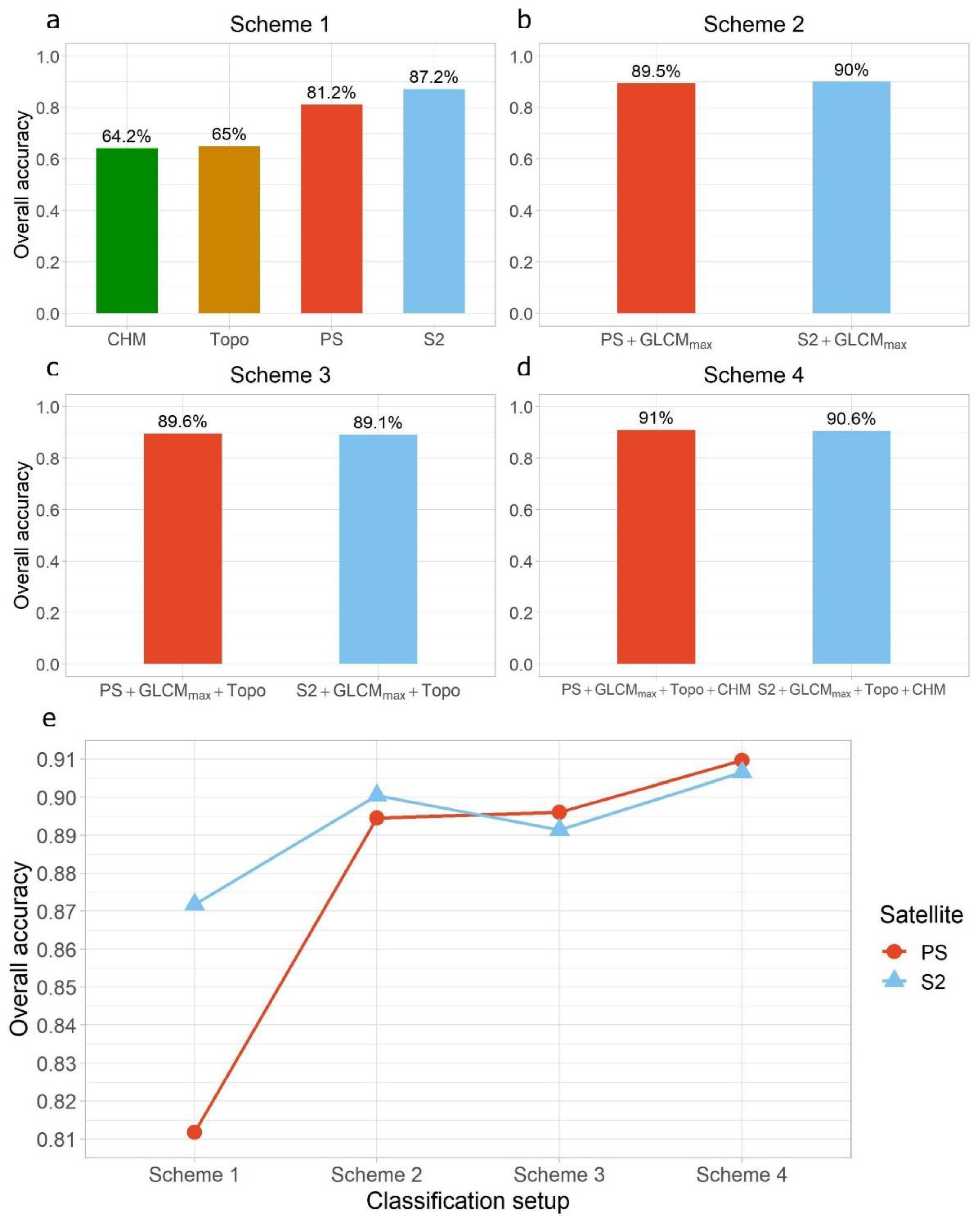
Figure 1. (a) Study area in Sarntal Valley with reference data points for mountain pines and other land cover classes. Blue stars indicate the locations of the field photography seen in c,d. Background: Orthophoto 2020 (Autonomous Province of Bolzano); (b) location of study area in South Tyrol, Italy. Basemap and Hillshade: OpenStreetMap, SRTM; (c,d) mountain pine fields in Durnholz Valley with visible clear-cuts. Pictures were taken during a field visit in July 2021 and (e) typical appearance of young, regrowing mountain pine. Picture was taken near location (d).
Remotesensing 14 03190 g001
Figure 2. (a) Study area (in yellow) and settlement areas (in red) in the Sarntal Alps with a black rectangle showing the extent of the example imagery in (bd). Background: Orthophoto 2020; (b) Orthophoto 2020 (20 cm) (Autonomous Province of Bolzano); (c) PlanetScope (5 July 2020) (3 m); (d) Sentinel-2 (7 July 2020) (10 m) and (e) Spectral signatures of grassland, mountain pines and coniferous forest. Spectral signatures are mean reflectance values from reference polygons within the extent of bd based on PlanetScope bands (5 July 2020).
Remotesensing 14 03190 g002aRemotesensing 14 03190 g002b
Figure 3. Methodology workflow for mountain pine mapping in the Sarntal Alps. A detailed description of the different feature spaces is given in Table 1. Each individual feature space of the respective classification schemes is classified using a Random Forest model. A subsequent majority filter generates the respective final output for the different feature spaces for the four classification schemes. For identifying the optimal GLCM window size (WS) for PS and S2 feature space, each GLCM WS feature space is classified and validated. The GLCM WS feature space with the highest overall accuracy is chosen as GLCMMAX for PlanetScope and Sentinel-2, respectively.
Remotesensing 14 03190 g003
Figure 4. Overall accuracies of mountain pine classifications based on PS and S2 (Table 1) feature spaces combined with different GLCM window sizes (in meter). GLCM window sizes were calculated from 3 × 3, 5 × 5, 7 × 7, 9 × 9, 11 × 11, 13 × 13, 15 × 15, 17 × 17, 23 × 23, 29 × 29, 35 × 35, 43 × 43 and 51 × 51 pixels for both PlanetScope and Sentinel-2 data (Section 2.3.1.).
Remotesensing 14 03190 g004
Figure 5. Overall accuracies of classification results for each feature space in: (a) classification scheme 1; (b) classification scheme 2; (c) classification scheme 3; (d) classification scheme 4 and (e) overall accuracy of PlanetScope and Sentinel-2 feature spaces in classification schemes 1–4.
Remotesensing 14 03190 g005
Figure 6. Mountain pine stands in the Durnholz Valley, classified by different feature space combinations. (a,c,e,g) Classification results based on PlanetScope feature spaces. Mountain pine areas derived from PlanetScope feature spaces are colored in red. (b,d,f,h) Classification results based on Sentinel-2 feature spaces. Mountain pine areas derived from Sentinel-2 feature spaces are colored in blue. Commission errors occur where pixels of other land cover classes are classified as mountain pines (false positive). Omission errors occur where mountain pine pixels are incorrectly not detected (false negative). Background: Orthophoto 2020 (Autonomous Province of Bolzano).
Remotesensing 14 03190 g006
Figure 7. ROC curves and AUC for different feature spaces of each classification scheme.
Remotesensing 14 03190 g007
Figure 8. (a) Classified mountain pine stands in the Sarntal Alps, South Tyrol. Displayed classification based on PS + GLCMMAX + Topo + CHM feature space (OA 91%). Background: Orthophoto 2020 (Autonomous Province of Bolzano); (bd) Zoom-in examples of classification result with indication of omission and commission errors.
Remotesensing 14 03190 g008
Figure 9. Landscape metrics for mountain pine stands in the Sarntal Alps, South Tyrol, based on final classification result (PS + GLCMMAX + Topo + CHM). (a) Surface area covered by mountain pines at different altitudes; (b) relative land cover of mountain pines at different altitudes; (c) surface area covered by mountain pines by cardinal direction; (d) surface area by mountain pine patches at different patch sizes.
Remotesensing 14 03190 g009
Table 1. Classification schemes and feature space description.
Classification SchemesFeature SpacesFeaturesNumber of LayersSpatial Resolution
Scheme 1PSMulti-temporal PlanetScope + NDVI203 m
S2Multi-temporal Sentinel-2 + NDVI2010 m
TopoElevation + slope + aspect33 m
CHMCanopy height model13 m
Scheme 2PS + GLCMMAXPS + GLCM statistics for optimal window size403 m
S2 + GLCMMAXS2 + GLCM statistics for optimal window size4010 m
Scheme 3PS + GLCMMAX + TopoPS + GLCM statistics for optimal window size + Topo433 m
S2 + GLCMMAX + TopoS2 + GLCM statistics for optimal window size + Topo4310 m
Scheme 4PS + GLCMMAX + Topo + CHMPS + GLCM statistics for optimal window size + Topo + CHM443 m
S2 + GLCMMAX + Topo + CHMS2 + GLCM statistics for optimal window size + Topo + CHM4410 m
Publisher’s Note: MDPI stays neutral with regard to jurisdictional claims in published maps and institutional affiliations.

