
Improved Object-Based Estimation of Forest Aboveground Biomass by Integrating LiDAR Data from GEDI and ICESat-2 with Multi-Sensor Images in a Heterogeneous Mountainous Region

 ,
, 

 , ,
, ,  and
and
Abstract
:
1. Introduction
2. Materials and Methods
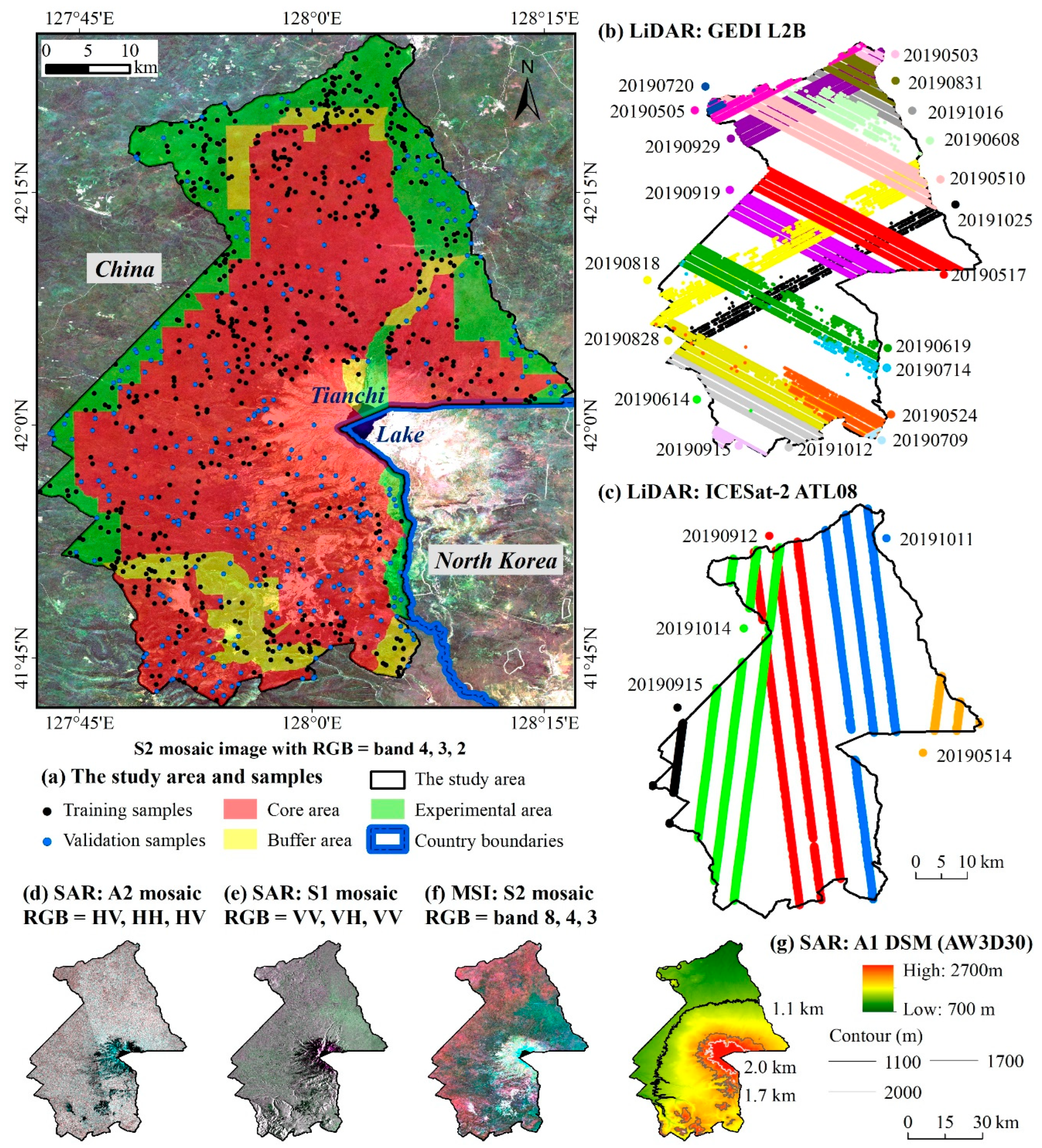
2.1. The Study Area
2.2. Data
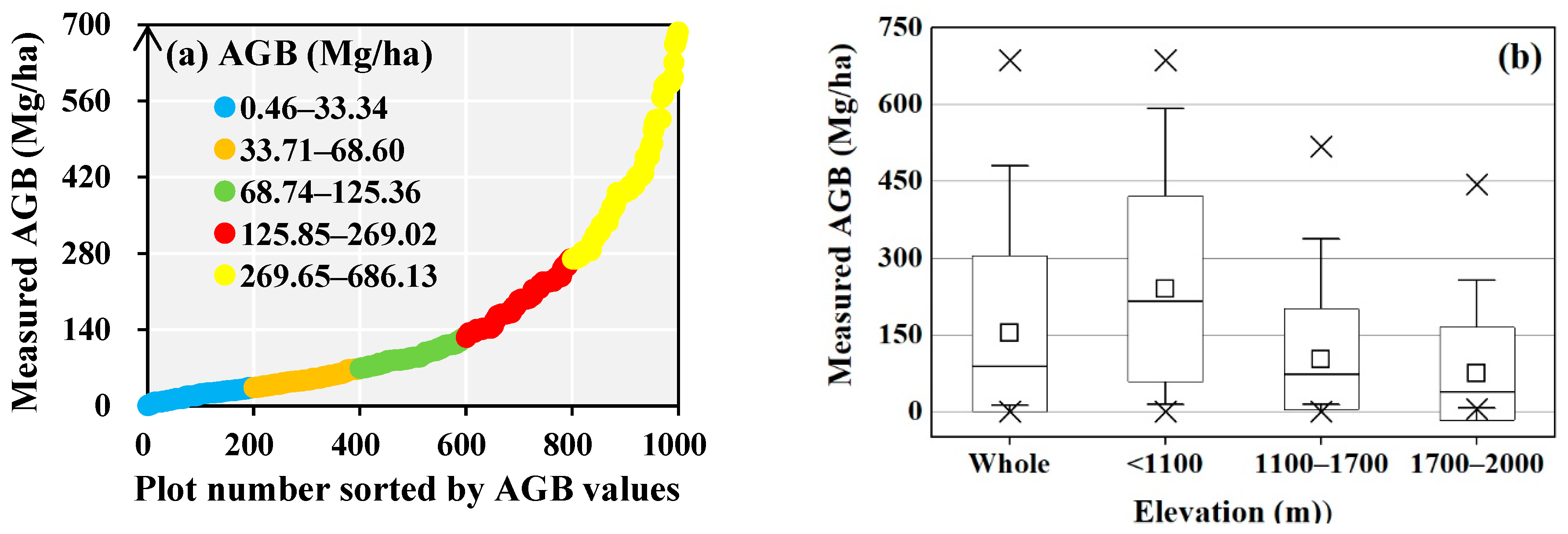
2.2.1. Field Data
2.2.2. LiDAR Data and Pre-Processing
2.2.3. Optical and SAR Images and Pre-Processing
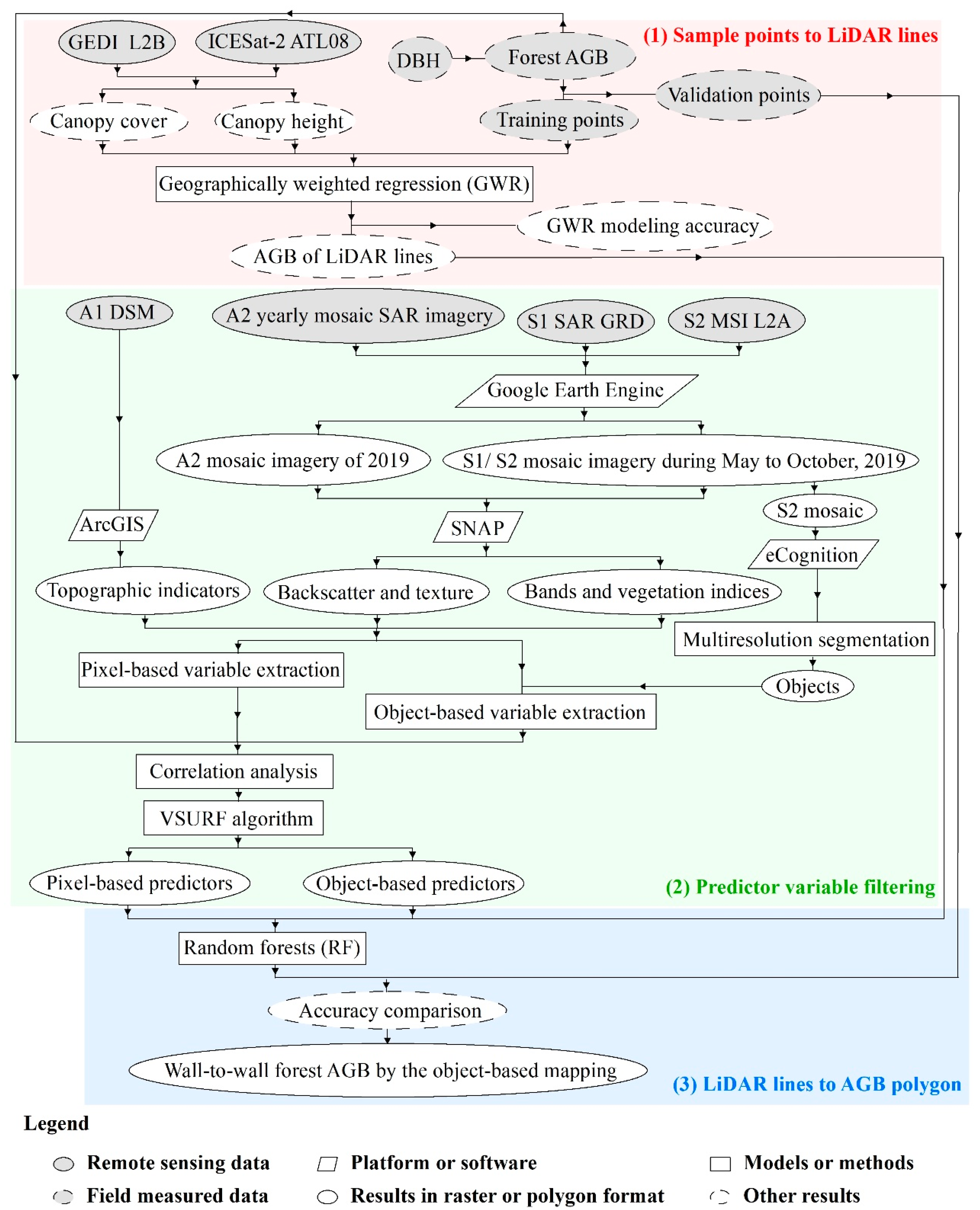
2.3. Methods
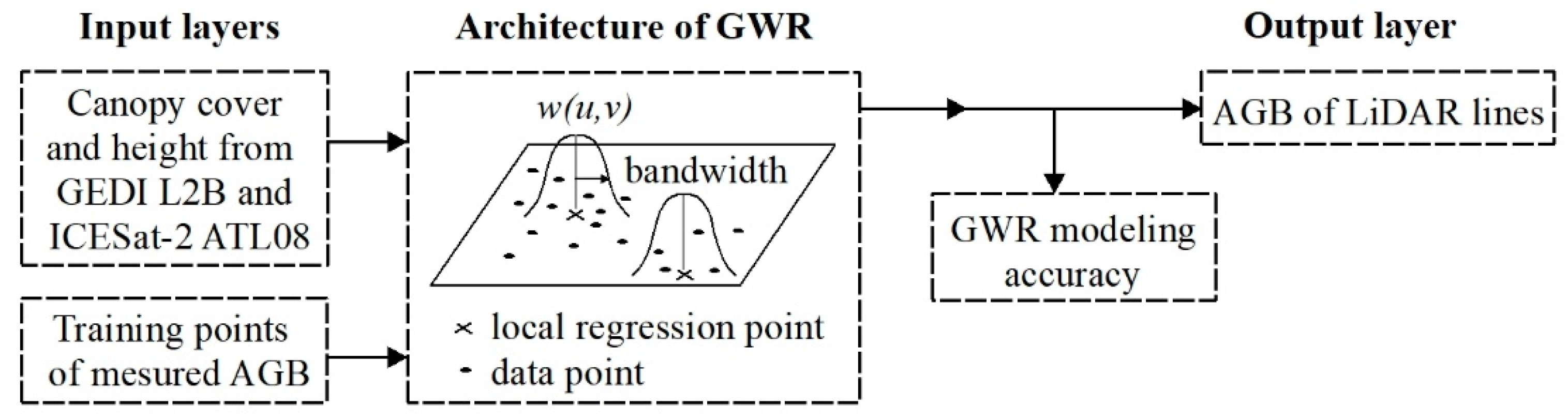
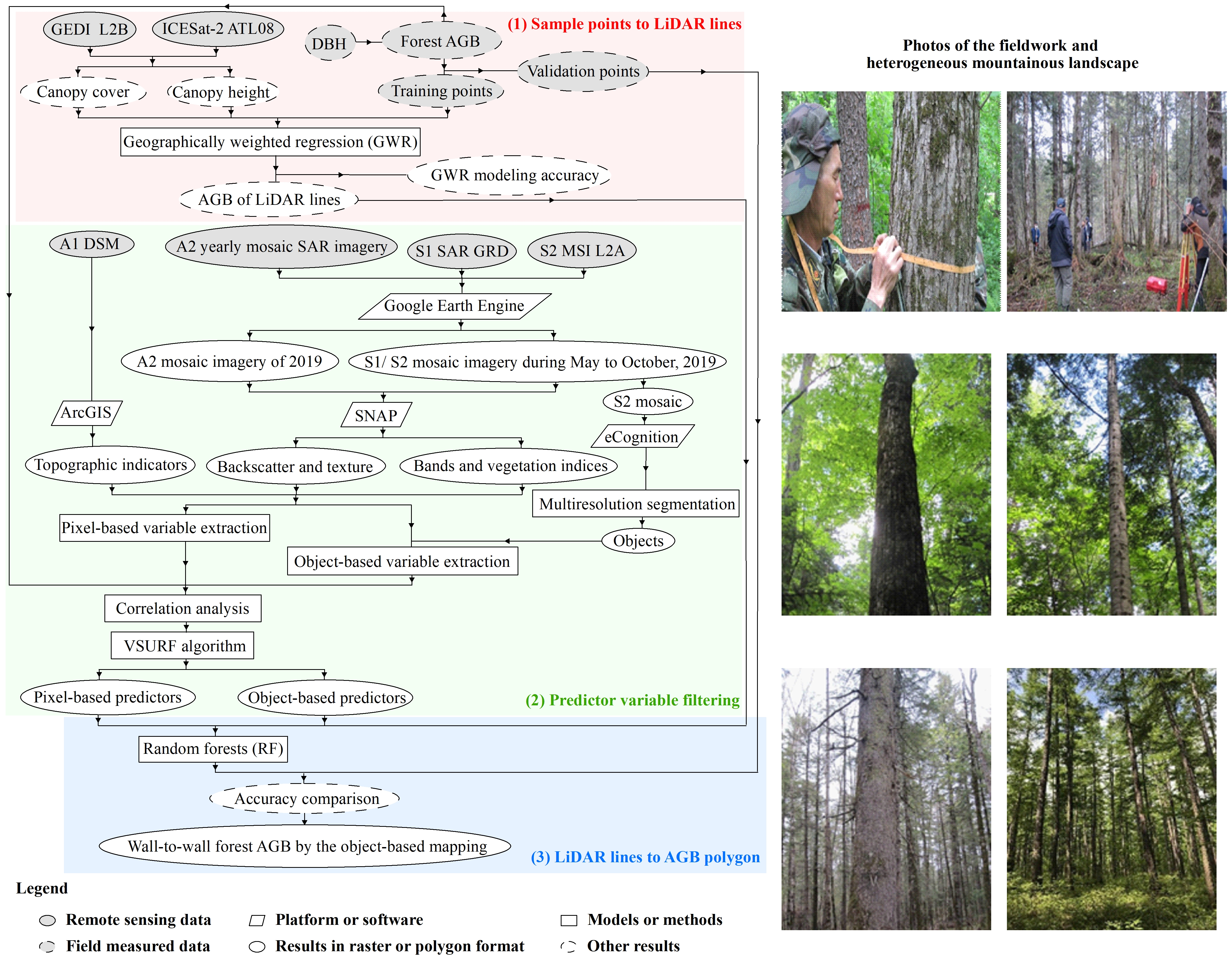
2.3.1. Estimation of AGB Lines from GEDI and ICESAT-2 Data by GWR
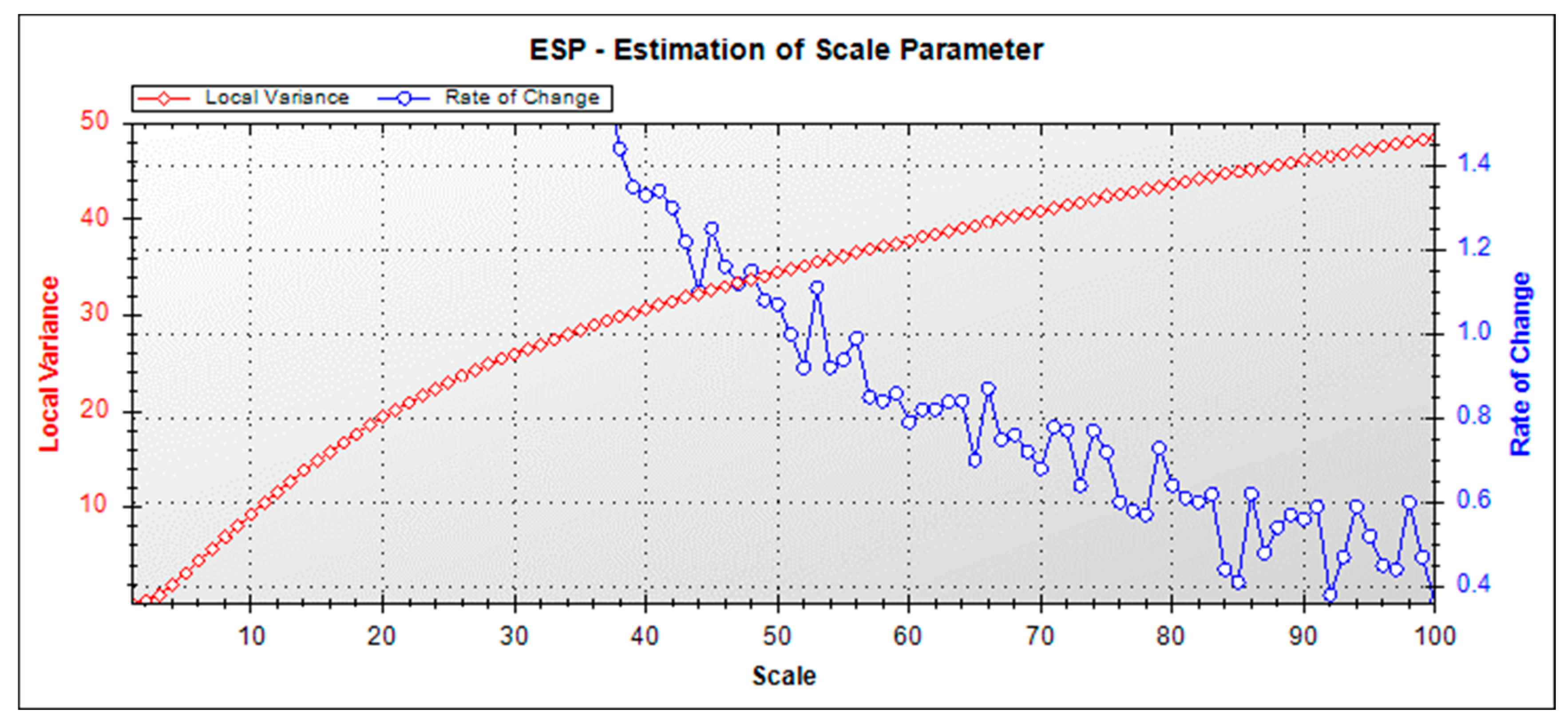
2.3.2. Filtering Predictors Based on Pixel- or Object-Based Analysis
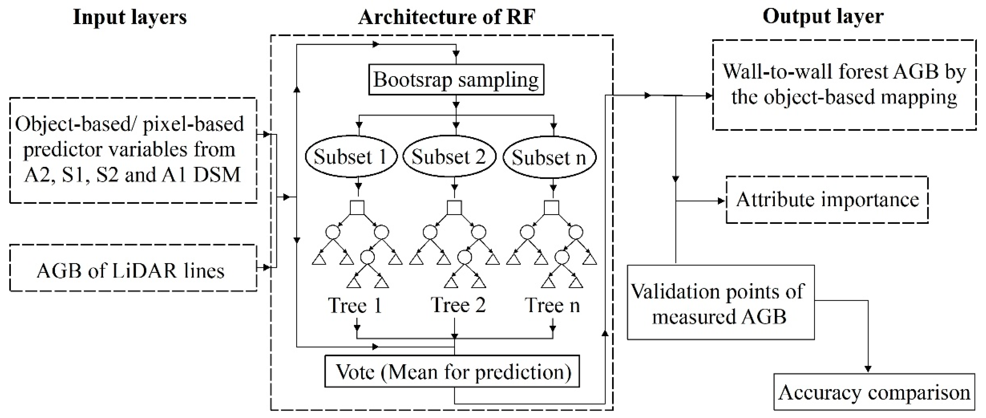
2.3.3. Mapping AGB Polygons from AGB Lines and Multi-Sensor Predictors by Random Forests
3. Results
3.1. The GWR Model and LiDAR-Based AGB Lines
3.2. Predictor Variables
3.3. Forest AGB in the CMNNR Mapped by RF Models
4. Discussion
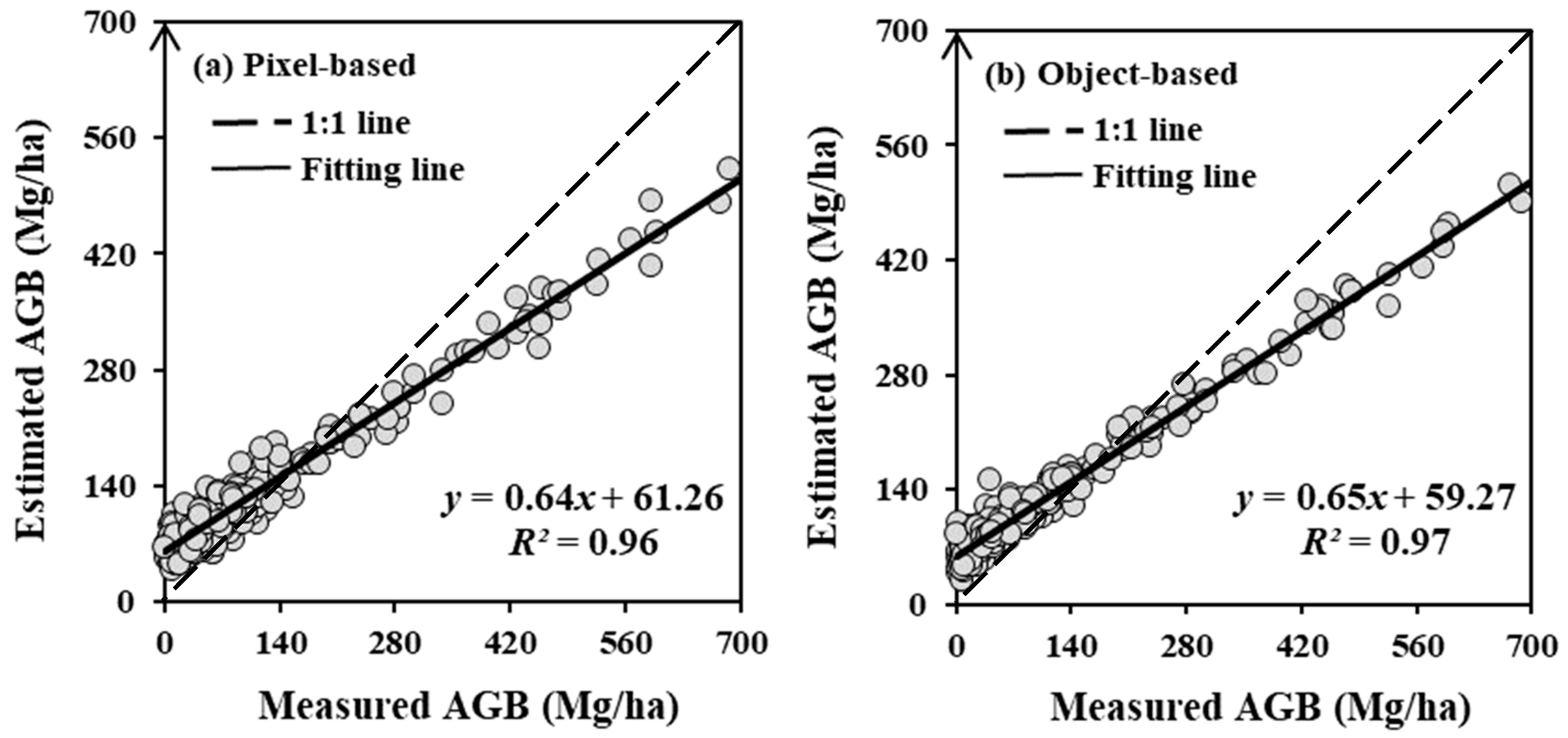
4.1. Pixel- versus Object-Based RF Modeling
4.2. Contributions of Multi-Sensor Variables to AGB Modeling
4.3. Uncertainty and Management in a Heterogeneous Mountain Landscape
5. Conclusions
- (1)
- The object-based approach accurately mapped AGB of heterogeneous forests in the CMNNR, and improved accuracy of 4.46% compared to the pixel-based process. The object-based approach also selected more optimized predictors and markedly decreased the prediction time compared to the pixel-based analysis.
- (2)
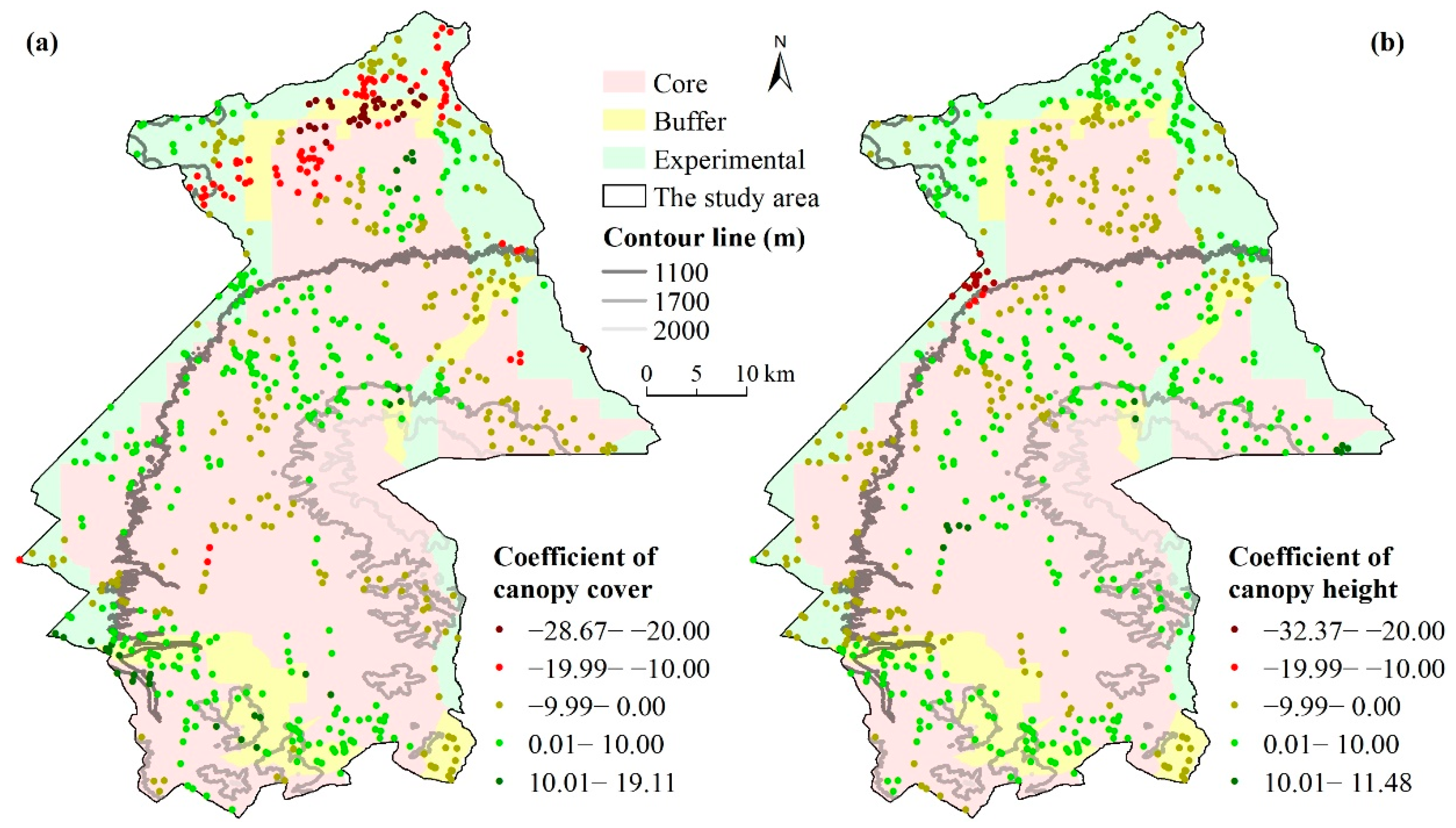
- Canopy cover and height explained forest AGB to a large extent (RMSE = 25.32%), and their effects on biomass varied by the elevation. The elevation from DSM and variables involved in red-edge bands from MSI were the most contributive predictors, and impacts of backscatters from C band SAR as well as their calculation were marginal.
- (3)
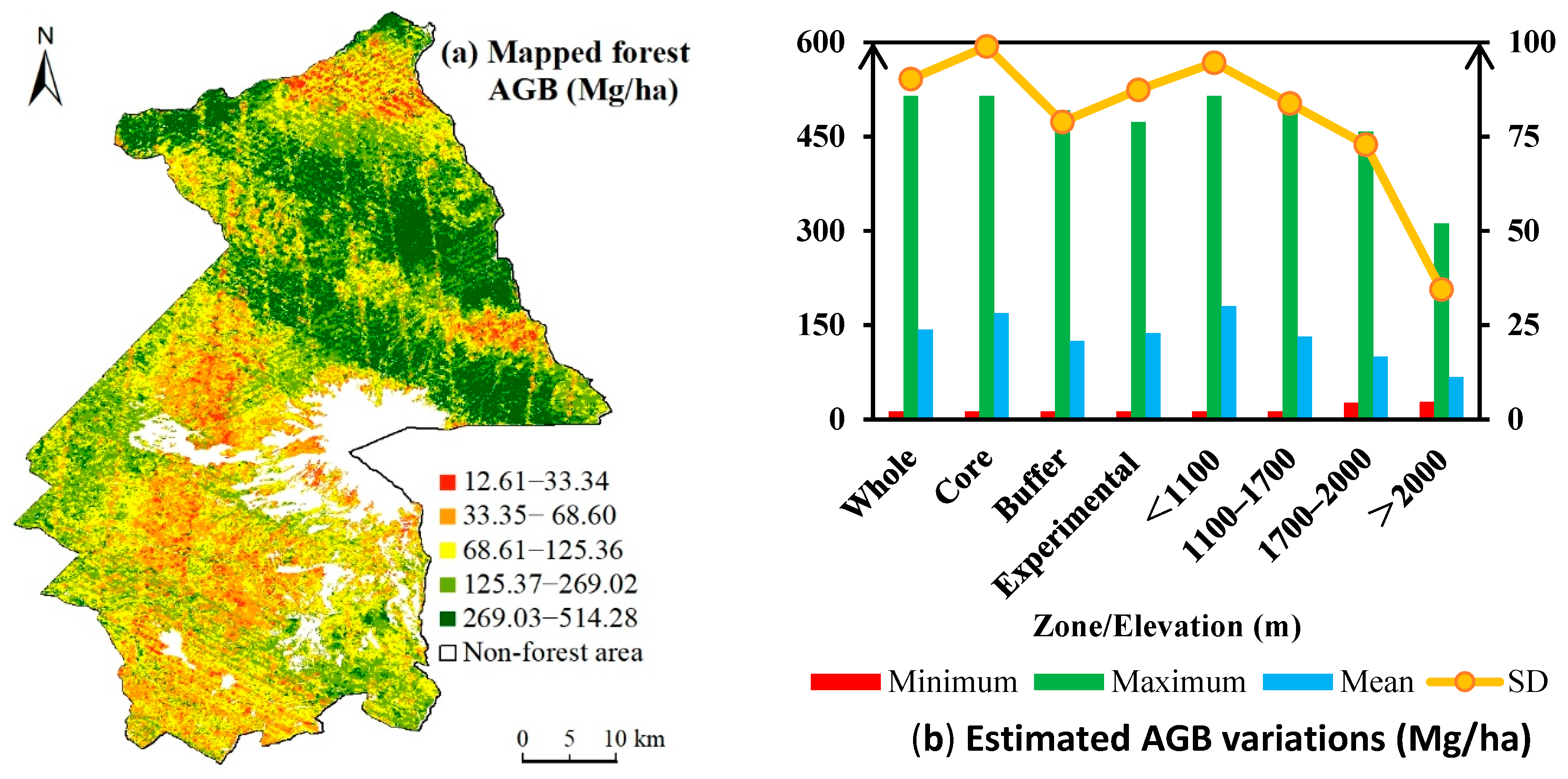
- The map illustrated that forest AGB of CMNNR varied along elevation gradients, with values from 12.61 to 514.28 Mg/ha. The north slope of the CMNNR with the lowest elevation (<1100 m) had the largest mean value, while forests in the south slope with the altitude above 2000 m had the smallest mean AGB. Forests in core areas had a much larger mean value of AGB than that in buffer and experimental zones.
Author Contributions
Funding
Data Availability Statement
Acknowledgments
Conflicts of Interest
References
- Lucas, R.M.; Mitchell, A.L.; Armston, J. Measurement of forest above-ground biomass using active and passive remote sensing at large (subnational to global) scales. Curr. For. Rep. 2015, 1, 162–177. [Google Scholar] [CrossRef] [Green Version]
- Yue, Q.; Hao, M.; Li, X.; Zhang, C.; von Gadow, K.; Zhao, X. Assessing biotic and abiotic effects on forest productivity in three temperate forests. Ecol. Evol. 2020, 10, 7887–7900. [Google Scholar] [CrossRef] [PubMed]
- Canadell, J.G.; Le Quéré, C.; Raupach, M.R.; Field, C.B.; Buitenhuis, E.T.; Ciais, P.; Conway, T.J.; Gillett, N.P.; Houghton, R.A.; Marland, G. Contributions to accelerating atmospheric CO2 growth from economic activity, carbon intensity, and efficiency of natural sinks. Proc. Natl. Acad. Sci. USA 2007, 104, 18866. [Google Scholar] [CrossRef] [PubMed] [Green Version]
- FAO. The State of the World’s Forests 2018—Forest Pathways to Sustainable Development. 2018. Rome. License: CC BY-NC-SA 3.0 IGO. Available online: http://www.fao.org/3/I9535EN/i9535en.pdf (accessed on 15 August 2019).
- Koju, U.A.; Zhang, J.; Maharjan, S.; Zhang, S.; Bai, Y.; Vijayakumar, D.B.I.P.; Yao, F. A two-scale approach for estimating forest aboveground biomass with optical remote sensing images in a subtropical forest of Nepal. J. For. Res. 2019, 30, 2119–2136. [Google Scholar] [CrossRef]
- Maltamo, M.; Bollandsås, O.M.; Gobakken, T.; Næsset, E. Large-scale prediction of aboveground biomass in heterogeneous mountain forests by means of airborne laser scanning. Can. J. For. Res. 2016, 46, 1138–1144. [Google Scholar] [CrossRef]
- Wang, Y.; Ni, W.; Sun, G.; Chi, H.; Zhang, Z.; Guo, Z. Slope-adaptive waveform metrics of large footprint lidar for estimation of forest aboveground biomass. Remote Sens. Environ. 2019, 224, 386–400. [Google Scholar] [CrossRef]
- Ene, L.T.; Naesset, E.; Gobakken, T.; Gregoire, T.G.; Stahl, G.; Holm, S. A simulation approach for accuracy assessment of two-phase post-stratified estimation in large-area LiDAR biomass surveys. Remote Sens. Environ. 2013, 133, 210–224. [Google Scholar] [CrossRef]
- Zhang, R.; Zhou, X.; Ouyang, Z.; Avitabile, V.; Qi, J.; Chen, J.; Giannico, V. Estimating aboveground biomass in subtropical forests of China by integrating multisource remote sensing and ground data. Remote Sens. Environ. 2019, 232, 111341. [Google Scholar] [CrossRef]
- Searle, E.B.; Chen, H.Y.H. Tree size thresholds produce biased estimates of forest biomass dynamics. For. Ecol. Manag. 2017, 400, 468–474. [Google Scholar] [CrossRef]
- Adnan, S.; Maltamo, M.; Mehtätalo, L.; Ammaturo, R.N.L.; Packalen, P.; Valbuena, R. Determining maximum entropy in 3D remote sensing height distributions and using it to improve aboveground biomass modelling via stratification. Remote Sens. Environ. 2021, 260, 112464. [Google Scholar] [CrossRef]
- Babcock, C.; Finley, A.O.; Andersen, H.E.; Pattison, R.; Cook, B.D.; Morton, D.C.; Alonzo, M.; Nelson, R.; Gregoir, T.; Ene, L.; et al. Geostatistical estimation of forest biomass in interior Alaska combining Landsat-derived tree cover, sampled airborne lidar and field observations. Remote Sens. Environ. 2018, 212, 212–230. [Google Scholar] [CrossRef] [Green Version]
- Liu, Y.; Gong, W.; Xing, Y.; Hu, X.; Gong, J. Estimation of the forest stand mean height and aboveground biomass in Northeast China using SAR Sentinel-1B, multispectral Sentinel-2A, and DEM imagery. ISPRS J. Photogram. Remote Sens. 2019, 151, 277–289. [Google Scholar] [CrossRef]
- Dube, T.; Mutanga, O. Evaluating the utility of the medium-spatial resolution Landsat 8 multispectral sensor in quantifying aboveground biomass in uMgeni catchment, South Africa. ISPRS J. Photogram. Remote Sens. 2015, 101, 36–46. [Google Scholar] [CrossRef]
- Lu, D.; Chen, Q.; Wang, G.; Liu, L.; Li, G.; Moran, E. A survey of remote sensing-based aboveground biomass estimation methods in forest ecosystems. Int. J. Digit. Earth 2016, 9, 63–105. [Google Scholar] [CrossRef]
- Karila, K.; Yu, X.; Vastaranta, M.; Karjalainen, M.; Puttonen, E.; Hyyppä, J. TanDEM-X digital surface models in boreal forest above-ground biomass change detection. ISPRS J. Photogram. Remote Sens. 2019, 148, 174–183. [Google Scholar] [CrossRef]
- Cartus, O.; Santoro, M.; Kellndorfer, J. Mapping forest aboveground biomass in the Northeastern United States with ALOS PALSAR dual-polarization L-band. Remote Sens. Environ. 2012, 124, 466–478. [Google Scholar] [CrossRef]
- Poorazimy, M.; Shataee, S.; McRoberts, R.E.; Mohammadi, J. Integrating airborne laser scanning data, space-borne radar data and digital aerial imagery to estimate aboveground carbon stock in Hyrcanian forests, Iran. Remote Sens. Environ. 2020, 240, 111669. [Google Scholar] [CrossRef]
- Ma, J.; Xiao, X.; Qin, Y.; Chen, B.; Hu, Y.; Li, X.; Zhao, B. Estimating aboveground biomass of broadleaf, needleleaf, and mixed forests in Northeastern China through analysis of 25-m ALOS/PALSAR mosaic data. For. Ecol. Manag. 2017, 389, 199–210. [Google Scholar] [CrossRef]
- Ningthoujam, R.K.; Joshi, P.K.; Roy, P.S. Retrieval of forest biomass for tropical deciduous mixed forest using ALOS PALSAR mosaic imagery and field plot data. Int. J. Appl. Earth Obs. Geoinf. 2018, 69, 206–216. [Google Scholar] [CrossRef]
- Carreiras, J.M.B.; Vasconcelos, M.J.; Lucas, R.M. Understanding the relationship between aboveground biomass and ALOS PALSAR data in the forests of Guinea-Bissau (West Africa). Remote Sens. Environ. 2012, 121, 426–442. [Google Scholar] [CrossRef]
- Baig, S.; Qazi, W.A.; Akhtar, A.M.; Waqar, M.M.; Ammar, A.; Gilani, H.; Mehmood, S.A. Above ground biomass estimation of Dalbergia sissoo forest plantation from dual-polarized ALOS-2 PALSAR data. Can. J. Remote Sens. 2017, 43, 297–308. [Google Scholar] [CrossRef]
- Castillo, J.A.A.; Apan, A.A.; Maraseni, T.N.; Salmo III, S.G. Estimation and mapping of above-ground biomass of mangrove forests and their replacement land uses in the Philippines using Sentinel imagery. ISPRS J. Photogram. Remote Sens. 2017, 134, 70–85. [Google Scholar] [CrossRef]
- Forkuor, G.; Zoungrana, J.B.B.; Dimobe, K.; Ouattara, B.; Vadrevu, K.P.; Tondoh, J.E. Above-ground biomass mapping in West African dryland forest using Sentinel-1 and 2 datasets—A case study. Remote Sens. Environ. 2020, 236, 111496. [Google Scholar] [CrossRef]
- Aslan, A.; Rahman, A.F.; Robeson, S.M. Investigating the use of Alos Prism data in detecting mangrove succession through canopy height estimation. Ecol. Indic. 2018, 87, 136–143. [Google Scholar] [CrossRef]
- Florinsky, I.V.; Skrypitsyna, T.N.; Luschikova, O.S. Comparative accuracy of the AW3D30 DSM, ASTER GDEM, and SRTM1 DEM: A case study on the Zaoksky testing ground, Central European Russia. Remote Sens. Lett. 2018, 9, 706–714. [Google Scholar] [CrossRef]
- Narine, L.L.; Popescu, S.; Neuenschwander, A.; Zhou, T.; Srinivasan, S.; Harbeck, K. Estimating aboveground biomass and forest canopy cover with simulated ICESat-2 data. Remote Sens. Environ. 2019, 224, 1–11. [Google Scholar] [CrossRef]
- Hernández-Stefanoni, J.L.; Castillo-Santiago, M.Á.; Mas, J.F.; Wheeler, C.E.; Andres-Mauricio, J.; Tun-Dzul, F.; George-Chacón, S.P.; Reyes-Palomeque, G.; Castellanos-Basto, B.; Vaca, R.; et al. Improving aboveground biomass maps of tropical dry forests by integrating LiDAR, ALOS PALSAR, climate and field data. Carbon Balance Manag. 2020, 15, 15. [Google Scholar] [CrossRef]
- Narine, L.L.; Popescu, S.; Zhou, T.; Srinivasan, S.; Harbeck, K. Mapping forest aboveground biomass with a simulated ICESat-2 vegetation canopy product and Landsat data. Ann. For. Res. 2019, 62, 69–86. [Google Scholar] [CrossRef]
- Dubayah, R.; Blair, J.B.; Goetz, S.; Fatoyinbo, L.; Hansen, M.; Healey, S.; Hofton, M.; Hurtt, G.; Kellner, J.; Luthcke, S.; et al. The Global Ecosystem Dynamics Investigation: High-resolution laser ranging of the Earth’s forests and topography. Sci. Remote Sens. 2020, 1, 100002. [Google Scholar] [CrossRef]
- Li, W.; Niu, Z.; Shang, R.; Qin, Y.; Wang, L.; Chen, H. High-resolution mapping of forest canopy height using machine learning by coupling ICESat-2 LiDAR with Sentinel-1, Sentinel-2 and Landsat-8 data. Int. J. Appl. Earth Obs. Geoinf. 2020, 92, 102163. [Google Scholar] [CrossRef]
- Potapov, P.; Li, X.; Hernandez-Serna, A.; Tyukavina, A.; Hansen, M.C.; Kommareddy, A.; Pickens, A.; Turubanova, S.; Tang, H.; Silva, C.E.; et al. Mapping global forest canopy height through integration of GEDI and Landsat data. Remote Sens. Environ. 2021, 253, 112165. [Google Scholar] [CrossRef]
- Duncanson, L.; Neuenschwander, A.; Hancock, S.; Thomas, N.; Fatoyinbo, T.; Simard, M.; Silva, C.A.; Armston, J.; Luthcke, S.B.; Hofton, M.; et al. Biomass estimation from simulated GEDI, ICESat-2 and NISAR across environmental gradients in Sonoma County, California. Remote Sens. Environ. 2020, 242, 111779. [Google Scholar] [CrossRef]
- Shen, W.; Li, M.; Huang, C.; Tao, X.; Wei, A. Annual forest aboveground biomass changes mapped using ICESat/GLAS measurements, historical inventory data, and time-series optical and radar imagery for Guangdong province, China. Agric. For. Meteorol. 2018, 259, 23–38. [Google Scholar] [CrossRef] [Green Version]
- Fayad, I.; Baghdadi, N.; Guitet, S.; Bailly, J.S.; Hérault, B.; Gond, V.; El Hajj, M.; Minh, D.H.T. Aboveground biomass mapping in French Guiana by combining remote sensing, forest inventories and environmental data. Int. J. Appl. Earth Obs. Geoinf. 2016, 52, 502–514. [Google Scholar] [CrossRef] [Green Version]
- Urbazaev, M.; Thiel, C.; Cremer, F.; Dubayah, R.; Migliavacca, M.; Reichstein, M.; Schmullius, C. Estimation of forest aboveground biomass and uncertainties by integration of field measurements, airborne LiDAR, and SAR and optical satellite data in Mexico. Carbon Balance Manag. 2018, 13, 5. [Google Scholar] [CrossRef] [Green Version]
- Wang, Y.; Zhang, X.; Guo, Z. Estimation of tree height and aboveground biomass of coniferous forests in North China using stereo ZY-3, multispectral Sentinel-2, and DEM data. Ecol. Indic. 2021, 126, 107645. [Google Scholar] [CrossRef]
- Huang, H.; Liu, C.; Wang, X.; Zhou, X.; Gong, P. Integration of multi-resource remotely sensed data and allometric models for forest aboveground biomass estimation in China. Remote Sens. Environ. 2019, 221, 225–234. [Google Scholar] [CrossRef]
- Wang, D.; Wan, B.; Liu, J.; Su, Y.; Guo, Q.; Qiu, P.; Wu, X. Estimating aboveground biomass of the mangrove forests on northeast Hainan Island in China using an upscaling method from field plots, UAV-LiDAR data and Sentinel-2 imagery. Int. J. Appl. Earth Obs. Geoinf. 2020, 85, 101986. [Google Scholar] [CrossRef]
- Silveira, E.M.O.; Silva, S.H.G.; Acerbi-Junior, F.W.; Carvalho, M.C.; Carvalho, L.M.T.; Scolforo, J.R.S.; Wulder, M.A. Object-based random forest modelling of aboveground forest biomass outperforms a pixel-based approach in a heterogeneous and mountain tropical environment. Int. J. Appl. Earth Obs. Geoinf. 2019, 78, 175–188. [Google Scholar] [CrossRef]
- Wang, Y.; Wu, Z.; Yuan, X.; Zhang, H.; Zhang, J.; Xu, J.; Lu, Z.; Zhou, Y.; Feng, J. Resources and ecological security of the Changbai Mountain region in Northeast Asia. In Remote Sensing of Protected Lands; Wang, Y.Q., Ed.; CRC Press: Boca Raton, FL, USA, 2011. [Google Scholar]
- Dai, L.; Jia, J.; Yu, D.; Lewis, B.J.; Zhou, L.; Zhou, W.; Zhao, W.; Jiang, L. Effects of climate change on biomass carbon sequestration in old-growth forest ecosystems on Changbai Mountain in Northeast China. For. Ecol. Manag. 2013, 300, 106–116. [Google Scholar] [CrossRef]
- Chen, L.; Ren, C.; Zhang, B.; Wang, Z.; Wang, Y. Mapping spatial variations of structure and function parameters for forest condition assessment of the Changbai Mountain National Nature Reserve. Remote Sens. 2019, 11, 3004. [Google Scholar] [CrossRef] [Green Version]
- Yang, X.; Xu, M. Biodiversity conservation in Changbai Mountain Biosphere Reserve, northeastern China: Status, problem, and strategy. Biodivers. Conserv. 2003, 12, 883–903. [Google Scholar] [CrossRef]
- Xu, Z.; Yu, G.; Zhang, X.; Ge, J.; He, N.; Wang, Q.; Wang, D. The variations in soil microbial communities, enzyme activities and their relationships with soil organic matter decomposition along the northern slope of Changbai Mountain. Appl. Soil Ecol. 2015, 86, 19–29. [Google Scholar] [CrossRef]
- Zhou, G.; Yi, G.; Tang, X.; Wen, Z.; Liu, C.; Kuang, Y.; Wang, W. Carbon Stock of Forest Ecosystems in China—Biomass Equations; Science Press: Beijing, China, 2018. [Google Scholar]
- Popescu, S.C.; Zhao, K.; Neuenschwander, A.; Lin, C. Satellite lidar vs. small footprint airborne lidar: Comparing the accuracy of aboveground biomass estimates and forest structure metrics at footprint level. Remote Sens. Environ. 2011, 115, 2786–2797. [Google Scholar] [CrossRef]
- Zald, H.S.J.; Wulder, M.A.; White, J.C.; Hilker, T.; Hermosilla, T.; Hobart, G.W.; Coops, N.C. Integrating Landsat pixel composites and change metrics with lidar plots to predictively map forest structure and aboveground biomass in Saskatchewan, Canada. Remote Sens. Environ. 2016, 176, 188–201. [Google Scholar] [CrossRef] [Green Version]
- Ni-Meister, W.; Jupp, D.L.B.; Dubayah, R. Modeling lidar waveforms in heterogeneous and discrete canopies. IEEE Trans. Geosci. Remote Sens. 2001, 39, 1943–1958. [Google Scholar] [CrossRef] [Green Version]
- Silva, C.A.; Hamamura, C.; Valbuena, R.; Hancock, S.; Cardil, A.; Broadbent, E.N.; Almeida, D.R.A.; Silva Junior, C.H.L.; Klauberg, C. rGEDI: NASA’s Global Ecosystem Dynamics Investigation (GEDI) Data Visualization and Processing, version 0.1.2. 2020. Available online: https://CRAN.R-project.org/package=rGEDI (accessed on 1 April 2020).
- Neuenschwander, A.; Pitts, K. The ATL08 land and vegetation product for the ICESat-2 Mission. Remote Sens. Environ. 2019, 221, 247–259. [Google Scholar] [CrossRef]
- NSIDC. ATL08 Product Data Dictionary. 2020. Available online: https://nsidc.org/sites/nsidc.org/files/technical-references/ICESat2_ATL08_data_dict_v003.pdf (accessed on 3 February 2020).
- Hird, J.N.; DeLancey, E.R.; McDermid, G.J.; Kariyeva, J. Google Earth Engine, open-access satellite data, and machine learning in support of large-area probabilistic wetland mapping. Remote Sens. 2017, 9, 1315. [Google Scholar] [CrossRef] [Green Version]
- Chen, L.; Ren, C.; Zhang, B.; Wang, Z.; Liu, M.; Man, W.; Liu, J. Improved estimation of forest stand volume by the integration of GEDI LiDAR data and multi-sensor imagery in the Changbai Mountains Mixed Forests Ecoregion (CMMFE), Northeast China. Int. J. Appl. Earth Obs. Geoinf. 2021, 100, 102326. [Google Scholar] [CrossRef]
- Aslan, A.; Rahman, A.F.; Warren, M.W.; Robeson, S.M. Mapping spatial distribution and biomass of coastal wetland vegetation in Indonesian Papua by combining active and passive remotely sensed data. Remote Sens. Environ. 2016, 183, 65–81. [Google Scholar] [CrossRef]
- Chen, L.; Wang, Y.; Ren, C.; Zhang, B.; Wang, Z. Assessment of multi-wavelength SAR and multispectral instrument data for forest aboveground biomass mapping using random forest kriging. For. Ecol. Manag. 2019, 447, 12–25. [Google Scholar] [CrossRef]
- Nie, S.; Wang, C.; Zeng, H.; Xi, X.; Li, G. Above-ground biomass estimation using airborne discrete-return and full-waveform LiDAR data in a coniferous forest. Ecol. Indic. 2017, 78, 221–228. [Google Scholar] [CrossRef]
- Bell, D.M.; Gregory, M.J.; Kane, V.; Kane, J.; Kennedy, R.E.; Roberts, H.M.; Yang, Z. Multiscale divergence between Landsat- and lidar-based biomass mapping is related to regional variation in canopy cover and composition. Carbon Balance Manag. 2018, 13, 15. [Google Scholar] [CrossRef] [Green Version]
- Brunsdon, C.; Fotheringham, A.S.; Charlton, M.E. Geographically weighted regression: A method for exploring spatial nonstationarity. Geogr. Anal. 1996, 28, 281–298. [Google Scholar] [CrossRef]
- Brunsdon, C.; Fotheringham, A.S.; Charlton, M.E. Geographically Weighted Regression–Modelling Spatial Non-stationarity. In Workshop on Local Indicators of Spatial Association; University of Leicester: Leicester, UK, 1998. [Google Scholar]
- Chen, L.; Ren, C.; Zhang, B.; Wang, Z.; Xi, Y. Estimation of forest above-ground biomass by geographically weighted regression and machine learning with Sentinel imagery. Forests 2018, 9, 582. [Google Scholar] [CrossRef] [Green Version]
- Fotheringham, A.S.; Brunsdon, C.; Charlton, M.E. Geographically Weighted Regression: The Analysis of Spatially Varying Relationships; Wiley: Chichester, UK, 2002. [Google Scholar]
- Nakaya, T.; Charlton, M.; Lewis, P.; Brunsdon, C.; Yao, J.; Fotheringham, S. GWR4 User Manual, Windows Application for Geographically Weighted Regression Modelling; Ritsumeikan University: Kyoto, Japan, 2014. [Google Scholar]
- Ahmed, M.A.A.; Abd-Elrahman, A.; Escobedo, F.J.; Cropper, W.P.; Martin, T.A.; Timilsina, N. Spatially-explicit modeling of multi-scale drivers of aboveground forest biomass and water yield in watersheds of the Southeastern United States. J. Environ. Manag. 2017, 199, 158–171. [Google Scholar] [CrossRef] [PubMed]
- Jia, M.; Mao, D.; Wang, Z.; Ren, C.; Zhu, Q.; Li, X.; Zhang, Y. Tracking long-term floodplain wetland changes: A case study in the China side of the Amur River Basin. Int. J. Appl. Earth Obs. Geoinf. 2020, 92, 102185. [Google Scholar] [CrossRef]
- Drǎguţ, L.; Tiede, D.; Levick, S.R. ESP: A tool to estimate scale parameter for multiresolution image segmentation of remotely sensed data. Int. J. Geogr. Inf. Sci. 2010, 24, 859–871. [Google Scholar] [CrossRef]
- Fassnacht, F.E.; Poblete-Olivares, J.; Rivero, L.; Lopatin, J.; Ceballos-Comisso, A.; Galleguillos, M. Using Sentinel-2 and canopy height models to derive a landscape-level biomass map covering multiple vegetation types. Int. J. Appl. Earth Obs. Geoinf. 2021, 94, 102236. [Google Scholar] [CrossRef]
- Genuer, R.; Poggi, J.-M.; Tuleau-Malot, C. VSURF: An R package for variable selection using random forests. R J. R Found. Stat. Comput. 2015, 7, 19–33. [Google Scholar] [CrossRef] [Green Version]
- Puliti, S.; Hauglin, M.; Breidenbach, J.; Montesano, P.; Neigh, C.S.R.; Rahlf, J.; Solberg, S.; Klingenberg, T.F.; Astrup, R. Modelling above-ground biomass stock over Norway using national forest inventory data with ArcticDEM and Sentinel-2 data. Remote Sens. Environ. 2020, 236, 111501. [Google Scholar] [CrossRef]
- Wittke, S.; Yu, X.W.; Karjalainen, M.; Hyyppä, J.; Puttonen, E. Comparison of two-dimensional multitemporal Sentinel-2 data with three dimensional remote sensing data sources for forest inventory parameter estimation over a boreal forest. Int. J. Appl. Earth Obs. Geoinf. 2019, 76, 167–178. [Google Scholar] [CrossRef]
- Laurin, G.V.; Pirotti, F.; Callegari, M.; Chen, Q.; Cuozzo, G.; Lingua, E.; Notarnicola, C.; Papale, D. Potential of ALOS2 and NDVI to estimate forest above-ground biomass, and comparison with Lidar-derived estimates. Remote Sens. 2017, 9, 18. [Google Scholar] [CrossRef] [Green Version]
- Sinha, S.; Santra, A.; Sharma, L.; Jeganathan, C.; Nathawat, M.S.; Das, A.K.; Mohan, S. Multi-polarized Radarsat-2 satellite sensor in assessing forest vigor from above ground biomass. J. For. Res. 2018, 29, 1139–1145. [Google Scholar] [CrossRef]
- Astola, H.; Häme, T.; Sirro, L.; Molinier, M.; Kilpi, J. Comparison of Sentinel-2 and Landsat 8 imagery for forest variable prediction in boreal region. Remote Sens. Environ. 2019, 223, 257–273. [Google Scholar] [CrossRef]
- Rodríguez-Veiga, P.; Quegan, S.; Carreiras, J.; Persson, H.J.; Fransson, J.E.S.; Hoscilo, A.; Ziółkowski, D.; Stereńczak, K.; Lohberger, S.; Stängel, M.; et al. Forest biomass retrieval approaches from earth observation in different biomes. Int. J. Appl. Earth Obs. Geoinf. 2019, 77, 53–68. [Google Scholar] [CrossRef]
- Silva, C.A.; Duncanson, L.; Hancock, S.; Neuenschwander, A.; Thomas, N.; Hofton, M.; Fatoyinbo, L.; Simard, M.; Marshak, C.Z.; Armston, J.; et al. Fusing simulated GEDI, ICESat-2 and NISAR data for regional aboveground biomass mapping. Remote Sens. Environ. 2021, 253, 112234. [Google Scholar] [CrossRef]
- Chi, H.; Sun, G.; Huang, J.; Li, R.; Ren, X.; Ni, W.; Fu, A. Estimation of forest aboveground biomass in Changbai Mountain region using ICESat/GLAS and Landsat/TM data. Remote Sens. 2017, 9, 707. [Google Scholar] [CrossRef] [Green Version]
- Shen, C.; Liang, W.; Shi, Y.; Lin, X.; Zhang, H.; Wu, X.; Xie, G.; Chain, P.; Grogan, P.; Chu, H. Contrasting elevational diversity patterns between eukaryotic soil microbes and plants. Ecology 2014, 95, 3190–3202. [Google Scholar] [CrossRef] [Green Version]
- Cong, Y.; Li, M.; Liu, K.; Dang, Y.; Han, H.; He, H. Decreased temperature with increasing elevation decreases the end-season leaf-to-wood reallocation of resources in deciduous Betula ermanii Cham. Trees. Forests 2019, 10, 166. [Google Scholar] [CrossRef] [Green Version]
- Yuan, Z.; Ali, A.; Jucker, T.; Ruiz-Benito, P.; Wang, S.; Jiang, L.; Wang, X.; Lin, F.; Ye, J.; Hao, Z.; et al. Multiple abiotic and biotic pathways shape biomass demographic processes in temperate forests. Ecology 2019, 100, e02650. [Google Scholar] [CrossRef] [PubMed] [Green Version]
- Puliti, S.; Saarela, S.; Gobakken, T.; Ståhl, G.; Naesset, E. Combining UAV and Sentinel-2 auxiliary data for forest growing stock volume estimation through hierarchical model-based inference. Remote Sens. Environ. 2018, 204, 485–497. [Google Scholar] [CrossRef]
- Sinha, S.; Jeganathan, C.; Sharma, L.K.; Nathawat, M.S. A review of radar remote sensing for biomass estimation. Int. J. Environ. Sci. Technol. 2015, 12, 1779–1792. [Google Scholar] [CrossRef] [Green Version]
- Morin, D.; Planells, M.; Guyon, D.; Villard, L.; Mermoz, S.; Bouvet, A.; Thevenon, H.; Dejoux, J.-F.; Toan, T.L.; Dedieu, G. Estimation and mapping of forest structure parameters from open access satellite images: Development of a generic method with a study case on coniferous plantation. Remote Sens. 2019, 11, 1275. [Google Scholar] [CrossRef] [Green Version]
- Lefsky, M.A.; Cohen, W.B.; Acker, S.A.; Parker, G.G.; Spies, T.A.; Harding, D. Lidar remote sensing of the canopy structure and biophysical properties of Douglas-Fir Western Hemlock Forests. Remote Sens. Environ. 1999, 70, 339–361. [Google Scholar] [CrossRef]
- Rodríguez-Veiga, P.; Saatchi, S.; Tansey, K.; Balzter, H. Magnitude, spatial distribution and uncertainty of forest biomass stocks in Mexico. Remote Sens. Environ. 2016, 183, 265–281. [Google Scholar] [CrossRef] [Green Version]


| Tree Species/Family/Types | Trunk | Branch | Leaf |
|---|---|---|---|
| Betula platyphylla Suk. | 0.1951 × DBH2.2398 | 0.0228 × DBH2.2723 | 0.0111 × DBH1.9708 |
| Tilia tuan Szyszyl. | 0.1286 × DBH2.2255 | 0.0445 × DBH1.9516 | 0.0197 × DBH1.6667 |
| Betula costata Trautv. | 0.1555 × DBH2.2273 | 0.0134 × DBH2.4932 | 0.0092 × DBH2.0967 |
| Populus L. | 0.2538 × DBH1.1815 | 0.0470 × DBH1.9739 | 0.0222 × DBH2.1885 |
| Ulmus pumila L. | 0.0971 × DBH2.3253 | 0.0278 × DBH2.3540 | 0.0239 × DBH2.0051 |
| Quercus L. | 0.1030 × DBH2.2950 | 0.0160 × DBH2.6080 | 0.0110 × DBH2.2170 |
| Pinus koraiensis Sieb. et Zucc. | 0.0418 × DBH2.5919 | 0.0208 × DBH1.9612 | 0.0873 × DBH1.3480 |
| Abies fabri (Mast.) Craib | 0.0543 × DBH2.4242 | 0.0255 × DBH2.0726 | 0.0773 × DBH1.5761 |
| Picea asperata Mast. | 0.0562 × DBH2.4608 | 0.1298 × DBH1.8070 | 0.1436 × DBH1.6729 |
| Pinus sylvestris var. mongolica Litv. | 0.1790 × DBH2.0310 | 0.0844 × DBH1.7692 | 0.0732 × DBH1.6675 |
| Larix gmelinii (Rupr.) Kuzen. | 0.0526 × DBH2.5257 | 0.0085 × DBH2.4815 | 0.0168 × DBH2.0026 |
| Other broad-leaved trees | 0.2266 × DBH2.1699 | 0.0121 × DBH2.5685 | 0.0229 × DBH1.9485 |
| Other coniferous trees | 0.0425 × DBH2.5971 | 0.0177 × DBH2.0585 | 0.0618 × DBH1.4771 |
| Source | Level | Spatial Resolution | Date | Elements |
|---|---|---|---|---|
| GEDI | 2B | 25 m | 20190503, 0505, 0510, 0517, 0524, 0530, 0608. 0614, 0619, 0630, 0709, 0714, 0720, 0804, 0813, 0818, 0828, 0831, 0910, 0915, 0919, 0929, 1012, 1016, 1025 | T1602, 2593, 1296, 1143, 2260, 5439, 1449, 4628, 2413, 0531, 4781, 3683, 3863, 1476, 4448, 4322, 3530, 0026, 0512, 3377, 2566, 1170, 0684, 4142, 2899 |
| ICESat-2 | ATL08 | 100 m | 20190514, 0912, 0915, 1011, 1014 | 07040306, 11690402, 12070406, 02240502, 02620506 |
| Source | Level | Spatial Resolution | Date | Elements |
|---|---|---|---|---|
| A2 | Yearly mosaic | 25 m | 2019 | N42E127, N42E128, N43E127, N43E128 |
| S1 | Ground Range Detected (GRD) scenes | 10 m | 20190504, 0511, 0523, 0604, 0616, 0628, 0710, 0722, 0803, 0815, 0827, 0901, 0908, 0913, 0920, 1002, 1014, 1026 | S1A_030CEC_4C1D, 3104D_C272, 315C5_F0B1, 31B36_F05C, 3207F_6155, 325B7_927A, 32B0B_9904, 33052_2FEE, 335A7_2036, 33B72_710E, 34189_6AF3, 34415_3340, 3479D_8BE2, 34A27_DC13, 34DA7_D875, 353AB_F55C, 359B8_7567, 35FB6_A688 |
| 20190503, 0508, 0515, 0520, 0527, 0601, 0608, 0613, 0620, 0625, 0702, 0714, 0719, 0726, 0731, 0807, 0812, 0819, 0831, 0905, 0912, 0917, 0924, 0929, 1006, 1011, 1018, 1023, 1030 | S1B_1E41C_F791, 1E671_C1F2, 1E9A3_E18A, 1EBD2_89DA, 1EEFF_9395, 1F128_5411, 1F438_AF2E, 1F65C_F904, 1F96F_3C04, 1FB87_96B7, 1FE9A_9303, 203C2_5BAE, 205CF_E75B, 208D7_5F71, 20B01_D973, 20E22_7E43, 2105F_D04A, 21398_0C46, 21909_5957, 21B40_2E33, 21E81_62C0, 220BA_841B, 223E8_0AF8, 2261D_DA49, 2296A_F309, 22B9B_574C, 22ECA_6BF5, 230F2_5472, 2343E_D938 | |||
| S2 | 2A, orthorectified atmospherically corrected surface reflectance | 10 m | 20190503, 0506, 0513, 0516, 0518, 0523, 0526, 0602, 0605, 0612, 0615, 0622, 0625, 0702, 0705, 0712, 0715, 0722, 0725, 0801, 0804, 0811, 0814, 0821, 0824, 0831, 0903, 0910, 0913, 0920, 0923, 0930, 1003, 1010, 1013, 1020, 1023, 1030 | There are three images on each date as S2A_T52TCM, T52TDM, and T52TDN. |
| 20190501, 0508, 0511, 0528, 0531, 0607, 0610, 0617, 0620, 0627, 0630, 0707, 0710, 0717, 0720, 0727, 0730, 0806, 0809, 0816, 0819, 0826, 0829, 0905, 0908, 0915, 0918, 0925, 0928, 1005, 1008, 1015, 1018, 1025, 1028 | There are three images on each date as S2B_T52TCM, T52TDM, and T52TDN. | |||
| A1 | DSM | 30 m | Derived from A1 SAR data during 2006 to 2011 | N41E127, N41E128, N42E127, N42E128 |
| Images | Variables | Description | |
|---|---|---|---|
| A2 mosaic | Backscatter | HH | Normalized backscatter coefficient of horizontal transmit-horizontal channel in dB |
| HV | Normalized backscatter coefficient of vertical transmit-vertical channel in dB | ||
| RFDI | Radar forest degradation index, (HH − HV)/(HH + HV) | ||
| V/H_L | HV/HH | ||
| S1 mosaic | Backscatter | VV | Normalized backscatter coefficient of vertical transmit-vertical channel in dB |
| VH | Normalized backscatter coefficient of vertical transmit-horizontal channel in dB | ||
| NP | Normalized polarization, (VH − VV)/(VH + VV) | ||
| V/H_C | VV/VH | ||
| Texture | VV/VH_CON | Contrast | |
| VV/VH_DIS | Dissimilarity | ||
| VV/VH_HOM | Homogeneity | ||
| VV/VH_ASM | Angular second moment | ||
| VV/VH_ENE | Energy | ||
| VV/VH_MAX | Maximum probability | ||
| VV/VH_ENT | Entropy | ||
| VV/VH_MEA | Gray-level co-occurrence matrix (GLCM) mean | ||
| VV/VH_VAR | GLCM variance | ||
| VV/VH_COR | GLCM correlation | ||
| S2 mosaic | Multispectral bands | B2 | Blue, 490 nm |
| B3 | Green, 560 nm | ||
| B4 | Red, 665 nm | ||
| B5 | Red edge, 705 nm | ||
| B6 | Red edge, 749 nm | ||
| B7 | Red edge, 783 nm | ||
| B8 | Near infrared, 842 nm | ||
| B8a | Near infrared, 865 nm | ||
| B11 | Short-wave infrared, 1610 nm | ||
| B12 | Short-wave infrared, 2190 nm | ||
| Vegetation indices | RVI | Ratio vegetation index, B8/B4 | |
| DVI | Difference vegetation index, B8 − B4 | ||
| NDVI | Normalized difference vegetation index, (B8 − B4)/(B8 + B4) | ||
| EVI | Enhanced vegetation index, 2.5 × (B8 − B4)/(B8 + 6 × B4 − 7.5 × B2 + 1) | ||
| S2REP | Sentinel-2 red-edge position index, 705 + 35 × [(B4 + B7)/2 − B5] × (B6 − B5) | ||
| REIP | Red-edge infection point index, 700 + 40 × [(B4 + B7)/2 − B5]/(B6 − B5) | ||
| SAVI | Soil adjusted vegetation index, 1.5 × (B8 − B4)/8 × (B8 + B4 + 0.5) | ||
| MTCI | Meris terrestrial chlorophyll index, (B6 − B5)/(B5 − B4) | ||
| MCARI | Modified chlorophyll absorption ratio index, [(B5 − B4) − 0.2 × (B5 − B3)] × (B5 − B4) | ||
| NDVI45 | Normalized difference vegetation index with bands 4 and 5, (B5 − B4)/(B5 + B4) | ||
| NDVI56 | Normalized difference vegetation index with bands 5 and 6, (B6 − B5)/(B6 + B5) | ||
| NDVI57 | Normalized difference vegetation index with bands 5 and 7, (B7 − B5)/(B7 + B5) | ||
| NDVI58a | Normalized difference vegetation index with bands 5 and 8a, (B8a − B5)/(B8a + B5) | ||
| NDVI67 | Normalized difference vegetation index with bands 6 and 7, (B7 − B6)/(B7 + B6) | ||
| NDVI68a | Normalized difference vegetation index with bands 6 and 8a, (B8a − B6)/(B8a + B6) | ||
| NDVI78a | Normalized difference vegetation index with bands 7 and 8a, (B8a − B7)/(B8a + B7) | ||
| DSM | Topographic indicators | H | Elevation |
| β | Slope | ||
| A | Aspect | ||
| M | Surface roughness, 1/cosβ | ||
| TWI | Topographic wetness index, Ln [Ac/tanβ], Ac is the catchment area directed to the vertical flow | ||
| SPI | Stream power index, Ln [Ac × tanβ × 100] | ||
| Variables | Minimum | Maximum | Mean | Medium | SD |
|---|---|---|---|---|---|
| C | 0.002 | 11.61 | 1.78 | 0.61 | 2.68 |
| Ht (m) | 1.76 | 45.91 | 22.84 | 24.45 | 7.55 |
| AGB (Mg/ha) | 0.39 | 684.09 | 179.50 | 151.48 | 117.99 |
| Images | Variables | r | VSURF-Selected Predictors | ||
|---|---|---|---|---|---|
| Pixel-Based | Object-Based | Pixel-Based | Object-Based | ||
| A2 mosaic | HH | 0.12 ** | 0.11 ** | No | No |
| HV | 0.17 ** | Yes | |||
| RFDI | −0.08 * | −0.12 ** | No | No | |
| V/H_L | 0.09 ** | 0.13 ** | No | No | |
| S1 mosaic | VV_DIS | 0.08 * | No | ||
| VV_HOM | −0.15 ** | −0.17 ** | No | No | |
| VV_ASM | −0.11 ** | −0.11 ** | No | No | |
| VV_ENE | −0.14 ** | −0.15 ** | No | No | |
| VV_MAX | −0.13 ** | −0.14 ** | No | No | |
| VV_ENT | 0.15 ** | 0.17 ** | No | No | |
| VV_MEA | 0.11 ** | 0.11 ** | Yes | Yes | |
| VV_COR | 0.17 ** | 0.19 ** | Yes | No | |
| VH_DIS | 0.06 * | No | |||
| VH_HOM | −0.14 ** | −0.16 ** | Yes | No | |
| VH_ASM | −0.11 ** | −0.11 ** | No | No | |
| VH_ENE | −0.13 ** | −0.14 ** | No | No | |
| VH_MAX | −0.13 ** | −0.14 ** | No | No | |
| VH_ENT | 0.14 ** | 0.16 ** | No | No | |
| VH_COR | 0.11 ** | 0.13 ** | Yes | No | |
| S2 mosaic | B2 | −0.11 ** | −0.10 ** | No | No |
| B3 | −0.16 ** | −0.17 ** | No | No | |
| B4 | −0.17 ** | −0.17 ** | No | No | |
| B5 | −0.15 ** | −0.15 ** | Yes | No | |
| B6 | 0.08 * | 0.09 ** | No | No | |
| B7 | 0.11 ** | 0.13 ** | No | No | |
| B8 | 0.09 ** | 0.10 ** | No | No | |
| B8a | 0.09 ** | 0.10 ** | No | No | |
| RVI | 0.23 ** | 0.25 ** | No | No | |
| DVI | 0.13 ** | 0.15 ** | No | No | |
| NDVI | 0.20 ** | 0.21 ** | No | No | |
| EVI | 0.15 ** | 0.17 ** | Yes | Yes | |
| S2REP | 0.21 ** | 0.23 ** | No | No | |
| REIP | 0.26 ** | 0.30 ** | No | No | |
| SAVI | 0.08 ** | 0.10 ** | No | No | |
| MTCI | 0.25 ** | 0.30 ** | No | Yes | |
| MCARI | 0.11 ** | 0.12 ** | No | No | |
| NDVI45 | 0.12 ** | 0.13 ** | No | Yes | |
| NDVI56 | 0.26 ** | 0.30 ** | No | Yes | |
| NDVI57 | 0.27 ** | 0.29 ** | No | Yes | |
| NDVI58a | 0.26 ** | 0.27 ** | Yes | No | |
| NDVI67 | 0.22 ** | 0.29 ** | No | No | |
| NDVI68a | 0.09 ** | 0.07 * | No | No | |
| NDVI78a | 0.15 ** | 0.28 ** | No | Yes | |
| DSM | H | −0.43 ** | −0.43 ** | Yes | Yes |
| A | −0.11 ** | No | |||
| M | 0.16 ** | 0.21 ** | No | No | |
| TWI | 0.22 ** | Yes | |||
| Modeling Approach | ME | RMSE | R2 | RIRMSE (%) | ||
|---|---|---|---|---|---|---|
| Mg/ha | % | Mg/ha | % | |||
| Pixel-based | –24.22 | –15.87 | 54.47 | 35.69 | 0.96 | 0 |
| Object-based | –23.44 | –15.36 | 52.04 | 34.10 | 0.97 | 4.46 |
| Variable Source | Bandwidth | AICc | RMSE (Mg/ha) |
|---|---|---|---|
| GEDI | 158.67 | 6560.47 | 41.67 |
| ICESat-2 | 147.84 | 1630.92 | 56.75 |
| Both | 104.33 | 8099.31 | 38.64 |
Publisher’s Note: MDPI stays neutral with regard to jurisdictional claims in published maps and institutional affiliations. |
© 2022 by the authors. Licensee MDPI, Basel, Switzerland. This article is an open access article distributed under the terms and conditions of the Creative Commons Attribution (CC BY) license (https://creativecommons.org/licenses/by/4.0/).
Share and Cite
Chen, L.; Ren, C.; Bao, G.; Zhang, B.; Wang, Z.; Liu, M.; Man, W.; Liu, J. Improved Object-Based Estimation of Forest Aboveground Biomass by Integrating LiDAR Data from GEDI and ICESat-2 with Multi-Sensor Images in a Heterogeneous Mountainous Region. Remote Sens. 2022, 14, 2743. https://doi.org/10.3390/rs14122743
Chen L, Ren C, Bao G, Zhang B, Wang Z, Liu M, Man W, Liu J. Improved Object-Based Estimation of Forest Aboveground Biomass by Integrating LiDAR Data from GEDI and ICESat-2 with Multi-Sensor Images in a Heterogeneous Mountainous Region. Remote Sensing. 2022; 14(12):2743. https://doi.org/10.3390/rs14122743
Chicago/Turabian StyleChen, Lin, Chunying Ren, Guangdao Bao, Bai Zhang, Zongming Wang, Mingyue Liu, Weidong Man, and Jiafu Liu. 2022. "Improved Object-Based Estimation of Forest Aboveground Biomass by Integrating LiDAR Data from GEDI and ICESat-2 with Multi-Sensor Images in a Heterogeneous Mountainous Region" Remote Sensing 14, no. 12: 2743. https://doi.org/10.3390/rs14122743
APA StyleChen, L., Ren, C., Bao, G., Zhang, B., Wang, Z., Liu, M., Man, W., & Liu, J. (2022). Improved Object-Based Estimation of Forest Aboveground Biomass by Integrating LiDAR Data from GEDI and ICESat-2 with Multi-Sensor Images in a Heterogeneous Mountainous Region. Remote Sensing, 14(12), 2743. https://doi.org/10.3390/rs14122743