Abstract
Hyperspectral image change detection (HSI-CD) is an interesting task in the Earth’s remote sensing community. However, current HSI-CD methods are feeble at detecting subtle changes from bitemporal HSIs, because the decision boundary is partially stretched by strong changes so that subtle changes are ignored. In this paper, we propose a superpixel-by-superpixel clustering framework (SSCF), which avoids the confusion of different changes and thus reduces the impact on decision boundaries. Wherein the simple linear iterative clustering (SLIC) is employed to spatially segment the different images (DI) of the bitemporal HSIs into superpixels. Meanwhile, the Gaussian mixture model (GMM) extracts uncertain pixels from the DI as a rough threshold for clustering. The final CD results are obtained by passing the determined superpixels and uncertain pixels through K-means. The experimental results of two spaceborne bitemporal HSIs datasets demonstrate competitive efficiency and accuracy in the proposed SSCF.
1. Introduction
1.1. Background of Hyperspectral Change Detection
Change detection (CD) is a sensing task that analyzes the bitemporal or multitemporal images for the identification of the changed scene over time. Recently, lots of satellite missions carrying hyperspectral sensors have been launched consecutively, which means hyperspectral images (HSIs) have become an important data source for Earth observation. The abundant spectral information can boost target detection [1,2,3], anomaly detection [4,5,6], and classification [7,8,9]. Binary hyperspectral image CD (HSI-CD) is a special task in which the final change map (change map) reflects the change or not at the pixel level, i.e., zeros denote unchanged regions, and ones indicate changed regions. Such tasks can be applied to disaster assessment [10,11], agriculture and forestry monitoring [12,13], urban expansion research [14,15], etc. The HSI-CD task consists of three steps: data preprocessing, change identification, and change map output and evaluation. Among them, change identification is the most important and challenging step. The changes can be divided into strong and subtle changes according to the change intensity [16]. Strong changes are associated with bitemporal HSIs that have significantly different spectral features. In contrast, subtle changes just have small differences in spectral features between the bitemporal HSIs. For example, during the transition of land cover from bare land to crop, different water contents or different growth rates of the crops indicate different changes, where the lower water content or slower growth rate corresponds to subtle changes. Furthermore, subtle changes may be induced by mixed pixels that are usually present in the edge areas of the HSIs, because the spatial resolution of HSIs is limited. The changes of partial endmembers in the mixed pixels belong to subtle changes. However, the detection of subtle changes is challenging. Since HSIs can provide intensive sampling of spectral features over a wide spectral range, it is possible to accurately monitor changes at fine spectral scales. That is, HSIs have the advantage of being able to characterize subtle changes.
To exploit changes, kinds of methods have been proposed, including supervised and unsupervised methods. The former ones are limited by the availability of ground truths. Contrarily, the later ones do not require any a priori information and have aroused wide attention. Furthermore, the accurate detection of subtle changes without a priori data and with a lower false alarm rate is an interesting and meaningful task for HSI-CD. Therefore, we focus on unsupervised methods. Unsupervised binary CD methods that are applicable for HSI-CD can be generally classified into four types: (a) image algorithm-based methods [17], (b) image transform-based methods [18], (c) HSI-CD specified methods [19], and (d) deep learning-based methods [20].
1.1.1. Image Algorithm-Based Methods
The image algorithm-based methods assume that changes lead to significant differences in gray pixel levels and thus directly perform algebraic operations on bitemporal HSIs to determine pixel changes. The simple and commonly used arithmetical operations are image subtraction [21], image regression [22], and image rationing [23]. One typical algorithm is the change vector analysis (CVA) [24], which uses spectral vector subtraction to analyze the differences in the spectral bands. Recently, some modified CVA algorithms have also been proposed [25,26]. Structural similarity (SSIM) is also introduced into the image similarity measurement based on structural information degradation [27] and then used for the HSI-CD in [28]. These methods directly detect pixel pairs independently, which makes them sensitive to noise and misalignment errors.
1.1.2. Image Transform-Based Methods
Image transformation-based methods transform images into a specific feature space to emphasize changed pixels and suppress unchanged ones. Principal component analysis (PCA) [29] is a common algorithm for dimensionality reduction. Nielsen et al. [30] proposed a multivariate alteration detection (MAD) method based on typical correlation analysis, which used linear transformations of bitemporal HSIs to maximize changes. MAD has been successfully applied to vegetation monitoring in HSIs [31]. Iterative reweighted MAD (IR-MAD) [32] is an expanded version of MAD in iterative form. In addition, the slow feature analysis (SFA) method extracts slowly changing features from a time series [33,34]. It can be used for HSI-CD by suppressing unchanged features and highlighting the changed features [35]. Iterative SFA (ISFA) [36] assigns high weights to invariant pixels during iteration so that they can play a greater role in feature extraction.
1.1.3. HSI-CD Specified Methods
Recently, many CD methods have been proposed specifically for HSI-CD. Chen et al. [37] proposed an HSI-CD model based on spectrally and spatially regularized low-rank and sparse decomposition. It improved the already established low-rank and sparse decomposition to implement HSI-CD. Wu et al. [38] proposed an HSI anomalous CD method based on joint-sparse representation. In this method, the background dictionary is constructed by randomly selecting background pixels from the image. Then, it uses the constructed background dictionary to capture changes. In addition, spectral unmixing is also widely used in the implementation of HSI-CD [39,40,41,42,43]. These methods use spectral unmixing to determine whether the pixel changes directly or indirectly.
The tensor decomposition reconstruction detector (TDRD) HSI-CD method [44] implements a Tucker decomposition and reconstruction strategy for bitemporal HSIs to form new HSIs with increased separability. A novel patch tensor-based CD method (PTCD) [45] considers the non-overlapping local similarity property to make full use of the spatial structure information of bitemporal HSIs. In [46], MaxtreeCD is first proposed to exploit multiple morphological attributes to fully explore the spatial information, then a spectral angle weighted-based local absolute distance (SALA) is designed to determine the spectral change. It is found that MaxtreeCD can detect the complete changes and have good detection performance.
1.1.4. Deep Learning-Based Methods
Deep learning has swept across the field of remote sensing image interpretation due to the significant advantages in deep feature representation and nonlinear problem modeling [47,48,49,50]. For unsupervised HSI-CD, the pseudo-labels generated with unsupervised model-driven methods are usually used for training an artificial neural net (ANN). Li et al. [51] proposed a noise modeling-based unsupervised HSI-CD framework, in which the noise model is used to purify pseudo-labels for the end-to-end training process. Song et al. [52] proposed an HSI-CD architecture based on a recurrent 3D fully convolutional network, in which the pseudo-labels were generated by principal component analysis (PCA) and spectral correlation angle (SCA). Wang et al. [53] proposed a general end-to-end 2-D CNN (GETNET) HSI-CD framework, in which mixed-affinity matrices were formed, and features were extracted for classification. The pseudo-labels of the GETNET were produced by CVA. Du et al. [54] proposed a DSFA framework that extracted unchanged paired pixels from the CVA as training samples. The two trained ANNs were used to transform the bitemporal images separately. The invariant pairwise pixels were suppressed, and the changed pairwise pixels were highlighted using SFA constraint. Li et al. [28] proposed an improved pseudo-label generation mechanism that utilized CVA and SSIM to jointly guide the pseudo-label generation, which can be called the self-generated credible labels method (SGCL). In this case, the simple ANN with a single convolution layer can obtain accurate CD results. However, the generalization of the method needs to be improved because it cannot achieve desirable results on complex datasets with various changes, and the quality of the pseudo-label depends on both CVA and SSIM. Sun et al. [55] designed a new population confidence-based sample selection method to extract better quality and diverse pseudo-labels. However, the method is time-consuming. The image difference (ID) algorithm and spectral unmixing (SU) manner were also used to generate pseudo-training data [56], and the performance of this method is heavily dependent on the quality of spectral unmixing. In addition, some methods do not rely on pseudo-labels to achieve unsupervised HSI-CD [57,58,59] but exploit the characteristics of HSIs and the power of neural networks.
1.2. Problem Statements
The detection of subtle changes is challenging. Subtle changes arise from changes in similar species or mixed image elements. In general, subtle changes refer to changes with small differences in spectral features, and such changes are easy to be ignored. Moreover, the intensity of spurious changes caused by spectral susceptibility to distortion is similarly small. Therefore, it is difficult to correctly detect subtle changes while suppressing false changes. In [60], the results of some HSI-CD methods based on real HSIs datasets were compared. It is found that the methods without a priori knowledge are hard to detect subtle changes.
The performance of unsupervised data-driven CD methods such as deep learning is limited by the accuracy of pseudo-label. Moreover, deep learning CD methods are difficult to apply practically due to the high computational resource requirements and high time costs. In contrast, for model-driven CD methods, the decision boundary is susceptible to strong changes. As a result, subtle changes are ignored. Specifically, the model-driven CD methods do not distinguish between strong changes and subtle changes during detection, so the threshold for capturing subtle changes is subject to the presence of strong changes. In this case, subtle changes with a change intensity lower than the threshold are ignored. Therefore, an effective model-driven CD method is expected to detect the subtle changes specific to HSI.
1.3. Contributions of the Paper
In this paper, HSI-CD is specifically considered for a clustering task. To detect the subtle changes accurately, we propose a concise and effective hyperspectral change detection framework named SSCF. In SSCF, a single superpixel is the data to be detected, and the uncertain pixel from GMM can be considered as a rough threshold, and then a comparison between the two is implemented using K-means. The main contributions are summarized as follows.
- We propose ingenious strategies to achieve the detection of subtle changes. SLIC in SSCF can spatially segment different changes according to the intensity of the changes, which greatly increases the possibility of subtle changes being detected. GMM in SSCF separates uncertain pixels from the whole image as a rough threshold to highlight changes and accurately capture subtle changes. Consequently, the experimental results show that SSCF is able to detect subtle changes without increasing the false alarm rate.
- Compared with the existing traditional methods, SSCF can achieve more accurate detection. Compared with deep learning methods, SSCF achieves higher accuracy and shorter detection time.
2. Methodology
The structure is shown in Figure 1. The input is the bitemporal HSIs, T1 and T2, and the output is the change map. SSCF consists of four key parts: (1) the difference image (DI) is obtained according to T1 and T2, (2) all superpixels are acquired using SLIC, (3) uncertain pixels are obtained using GMM as a rough threshold, and (4) K-means clustering is used to obtain CD results for individual superpixels. The number of clustering is equal to the number of superpixels, and all results from all superpixels are assembled into a complete change map.
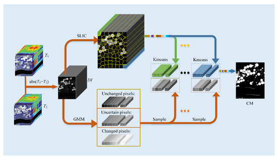
Figure 1.
The proposed SSCF for change detection of HSIs.
In this section, we describe, in detail, the basic principles of SLIC and GMM, as well as the process of SSCF.
2.1. SLIC
Superpixel segmentation can divide an image into non-overlapping superpixels, and each superpixel consists of a set of pixels with a similar color or other low-level cues. It is a useful preprocessing step in various HSIs processing and computer vision applications. Among the various superpixel algorithms, the simple linear iterative clustering (SLIC) algorithm [61] outperforms others in terms of computational complexity, storage efficiency, boundary consistency, undivided error, and boundary error. Specifically, SLIC provides a tradeoff between superpixels compactness control and boundary consistency.
SLIC is a superpixel segmentation algorithm inspired by K-means clustering. It is first introduced for RGB images, which converts the image from RGB color space to CIELAB. Then SLIC divides the CIELAB image into non-overlapping regions, which are controllable in size and compactness.
The first step is initialization. We initialize B clustering centers in a regular grid. To make the size of each superpixel consistent, the grid spacing should be , where N is the number of pixels and B is the number of superpixels. Then the gradient values of all pixels in the neighborhood 3 × 3 are calculated, and the clustering center is moved to the place with the smallest gradient in that neighborhood. This operation can avoid the clustering center falling on the contour boundary with a large gradient, which may affect the subsequent clustering effect.
The second step is assignment. This step assigns clustering centers to pixels. The desired superpixel size is set as S × S, and the search area is limited to 2S × 2S around the cluster center. By evaluating the specific distances of all pixels from the cluster center in the search area, the pixels are then specified to the nearest cluster center. The limited search area instead of all of the area is the key to speeding up the efficiency of the SLIC segmentation method. This is the significant difference between SLIC and K-means, where the search area of K-means clustering is not limited, i.e., each pixel must be compared with all cluster centers. Let the pixel of the image be expressed as , where represents the CIELAB color space and denotes the spatial position. Then, two distance s between pixel i and cluster center (pixel j) are defined as:
where dc and ds are color distance and spatial distance, respectively. The two distances are normalized and combined into the total distance D’:
where S becomes the maximum spatial distance, and w is a constant indicating the maximum color distance. Then, D′ is simplified to the specific distance:
In this case, w is allowed to measure the relative importance between color similarity and spatial proximity. If compactness w is larger, the spatial proximity is more important, and the resulting superpixels are more compact (i.e., they have a lower area to perimeter ratio). If compactness w is smaller, the resulting superpixels adhere more tightly to the image boundaries but do not have a regular size and shape. When using the CIELAB color space, compactness w can be in the range 1–40. A detailed interpretation of D′ can be found in [61].
The third step is update. The second step has grouped all pixels into their corresponding superpixels based on distances. However, once each pixel is assigned to the nearest cluster center, it is necessary to update the cluster center. Therefore, the third step needs to calculate the new cluster centers. The new cluster center is the average of all pixels’ vectors specified to the previous cluster center. L2norm is used to compute the residual E between the new cluster center and the previous cluster center. The assignment and update steps can be repeated iteratively until the error converges. Finally, the post-processing step enhances the connectivity by reassigning the disconnected pixels to nearby superpixels.
2.2. GMM
The Gaussian mixture model (GMM) is an effective statistical model that can be used for clustering data into several finite components. It assumes that each component belongs to a Gaussian distribution, and the whole components become a Gaussian mixture distribution. GMM is first proposed for background subtraction [62]. Thus far, it has been used in the field of image processing.
GMM assumed that an image is a mixture of K Gaussian distributions. Let each pixel on the image be expressed as over M bands. Then the assembly of all N pixels on the image is . In this case, the probability density function of is modeled as
where is the mixture parameter that satisfies and , and consists of the mean , and covariance matrix of the kth Gaussian distribution . The parameters determine the joint probability of the assemble using the likelihood function
Correspondingly, the log-likelihood expression is
Then, is estimated with maximum likelihood estimate (MLE) as
The expectation-maximization (EM) algorithm is effective for the MLE of mixture models. It can fit the GMM to the observed data by maximizing the log-likelihood function with respect to the parameters of the model (mean, covariance, and prior probability). The EM algorithm is based on the interpretation of is incomplete data. Herein, the affiliation of to the specific GMM components is unknown. We let this incompletion be a set of latent vectors with . If is generated from the kth component, , otherwise . Then the log-likelihood of the complete data is defined as
Finally, the EM algorithm iterates both the E-step and the M-step until the likelihood function converges to a certain optimal value.
E-step:
Due to the existence of the latent variable , a conditional expectation is defined
where is the parameter estimated by the current iteration t. Using the Bayes theorem, it is easy to draw the following formula
where
The probabilistic assignment can achieve the clustering of each pixel.
M-step:
Maximizing the expectation of the log-likelihood function, i.e., updating by maximizing the Q-function
2.3. Proposed SSCF Method
The difference image (DI) between the bitemporal HSIs, T1 and T2, is defined as
where each pixel in the DI corresponds to an M-dimensional spectral change vector (SCV). The DI characterizes the change intensity of each pixel in all bands. Therefore, The DI replaces the bitemporal HSI for subsequent detection.
Since the DI is a 3D data cube equal in size to bitemporal HSIs, SLIC theory for RGB images cannot be used directly for the DI. To make SLIC applicable to 3D data, the spectral distance needs to be measured explicitly, and the rest remains the same. Let each pixel on the DI be expressed as , where denotes SCV over M bands, and indicates the pixel’s spatial position. Then, the spectral distance between pixel i and cluster center (pixel j) is defined as:
It is found that the Euclidean distance metric is the most suitable one in SLIC to tackle high-dimensional vectors [61]. The DI is segmented by SLIC into B superpixels, which can be indicated as .
Figure 2 shows the segmentation result using SLIC on the fifth band DI of the USA dataset. As seen, the pixels in the boxed circular area have a similar color in each of the three images. That means the circular area is a superpixel and the changes in the pixels in this superpixel are similar. Therefore, SLIC can successfully separate different variations in the spatial dimension.
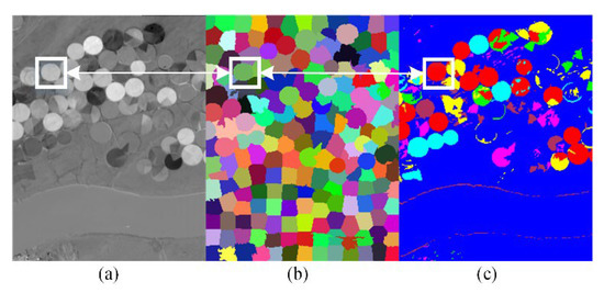
Figure 2.
The function of SLIC. (a) The fifth band DI of the USA dataset, (b) SLIC segmented superpixels with different colors, (c) the ground-truth for multiple change classes with different colors. The boxed circular area in each image is the same position.
The GMM assumed that the DI is a mixture of K = 3 Gaussian distributions. Let each pixel on the DI be expressed as over M bands. Then the assembly of all N pixels on the DI is . In this case, GMM divides the into K = 3 components: unchanged pixels, uncertain pixels, and changed pixels, as shown in Figure 3. Where the uncertain pixels are denoted as .
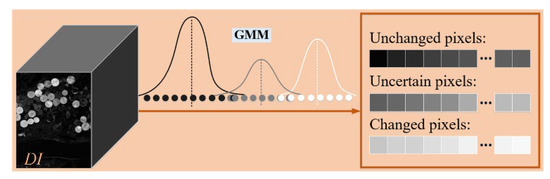
Figure 3.
The schematic diagram of GMM in SSCF.
After obtaining the superpixels, , and uncertain pixels, , K-means clustering is used to determine the superpixels. K-means reassigns all pixels of sp and un to two classes, changed and unchanged. The determination process can be expressed as
When sp is overall greater or less than un, sp is simply determined as changed pixels or unchanged pixels, respectively, and the two clustering centers are from sp and un, respectively. When sp is slightly different from un, the determination of sp is challenged, and the source of the clustering center needs to be constantly updated.
It should be noted that the ground truth for multiple change classes with different colors in Figure 2c is to verify that the superpixel segmentation can split the different changes. However, the number of components in GMM is set as three classes to extract the uncertainty pixels as a rough threshold during clustering. That is, the uncertain pixels extracted by GMM are used to cluster superpixels segmented by SLIC.
A flow chart of the proposed SSCF algorithm is shown in Figure 4. The important parameters involved are the number of superpixels and the compactness w in SLIC. The relevant hyperspectral tasks empirically set the number of superpixels and the compactness to [50, 100, 150, … 500] and [0, 0.1, … 1]. These parameter settings are also adaptable to any bitemporal HSIs. The selection of the number of superpixels parameters depends on the complexity of the ground feature. The choice of the compactness parameter depends on the contrast of the image and the shape of the ground feature. The optimal choice of the parameters differs for different HSI datasets. In any case, neither parameter has a decisive influence on the results.
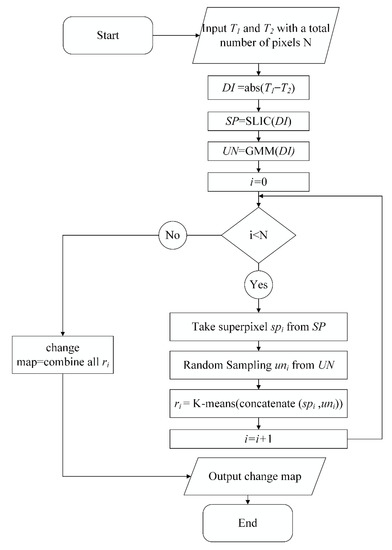
Figure 4.
The flow chart of the proposed SSCF algorithm.
3. Experiment
3.1. Datasets
Two main aspects should be considered in the selection of the datasets. The first is the availability of ground-truth data. Only high-quality and reliable ground-truth data are available to accurately assess the model’s performance. The second is the diversity among the datasets. Both simple and complex datasets are required to fully validate the generalization capability of the model. In terms of these points, two real-world HSIs datasets are used to evaluate the performance of SSCF [16,60], both of which have been widely used for the evaluation of existing HSI-CD efforts. Both datasets were acquired by the Hyperion sensor mounted onboard the EO-1 satellite and open access via the website (http://rslab.ut.ac.ir, accessed on 1 February 2022) [63]. They have a swath width of 7.7 km with a spatial resolution of 30 m and a spectral range of 0.4–2.5 µm with a spectral resolution of 10 nm [64,65].
As shown in Figure 5, each dataset consists of three elements: bitemporal HSIs and binarized ground-truth change map. The white pixels in the ground-truth change map indicate the changed classes, and the black pixels indicate the unchanged classes. The two datasets are described in detail as follows.
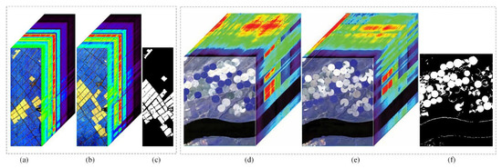
Figure 5.
Experimental datasets. (a) China imagery on 3 May 2006. (b) China imagery on 23 April 2007. (c) Ground-truth change map of the China dataset. (d) USA imagery on 1 May 2004. (e) USA imagery on 8 May 2007. (f) Ground-truth change map of the USA dataset.
The first dataset (China) is farmland near the city of Yancheng Jiangsu province in China, which was acquired on 3 May 2006 and 23 April 2007 [66]. This scene is mainly a combination of soil, rivers, trees, buildings, roads, and agricultural fields. Almost all the changes in this area are related to changes in the crop and soil in the fields. Each HSI has 155 bands with a spatial size of 450 × 140 pixels. While the changed regions contain 18,277 pixels, the unchanged regions contain 42,723 pixels.
The second dataset (USA) belongs to an irrigated agricultural field of Hermiston city in Umatilla County, Oregon, OR, the USA, which was acquired on 1 May 2004 and 8 May 2007 [60]. The land cover types are soil, irrigated fields, rivers, buildings, types of cultivated land, and grassland. Almost all the changes in this area are related to changes in the crop, soil, or water content (caused by different amounts of irrigated water) in the fields. Each HSI has 154 bands with a spatial size of 307 × 241 pixels. The changed regions contain 16,676 pixels, whereas the unchanged regions contain 57,311 pixels.
Both datasets have their own specific changes. Figure 6 shows the heatmap of DI in the 14th band and multiple SCVs from specified pixels. The heatmap visually reflects the change intensity of each pixel, and the SCV reflects the changes. The SCVs belong to three ground-truth changed pixels (C1, C2, C3) in the China dataset, six ground-truth changed pixels (C1, C2, …, C6) in the USA dataset, and two ground-truth unchanged pixels (UCs).
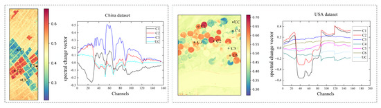
Figure 6.
The heatmap of DI in the 14th band and multiple SCVs from specified pixels.
As seen, the heatmap of the USA dataset contains more colors, which means the changes are more diverse. Both datasets have subtle changes, such as C2 in the China dataset and C4 and C5 in the USA dataset. Since the SCVs of these pixels are very close to UC, it is challenging to detect these points. Therefore, the separation of different changes becomes necessary and meaningful.
3.2. Parameter Setup
The performance of our proposed model SSCF is compared with seven existing HSI-CD methods (CVA [24], SSIM [27], ISFA [37], IRMAD [32], MaxtreeCD [46], Unet [67], SGCL [28]). The code of the MaxtreeCD method is implemented with Matlab, and other methods are implemented with Python.
SLIC segments the DI into specified 300 superpixels spatially with the compactness of 1. GMM divides the DI image into K = 3 components: unchanged pixels, uncertain pixels, and changed pixels. Figure 7 shows the pixels’ number and percentage of each component. As can be seen, the uncertain pixels occupy a large percentage, which are more than the test pixels in each superpixel (detection unit). To reduce the computational effort, only a fraction of the uncertain pixels are randomly selected as a rough threshold. The fraction selection experiments are implemented in Section 4. It is found that 10% of the uncertain pixels are good candidates and will be used in the comparison experiments. These 10% uncertain pixels are selected completely randomly without any dependence.
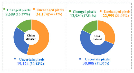
Figure 7.
Statistical information of K = 3 components: unchanged pixels, uncertain pixels, and changed pixels.
3.3. Evaluations Measures
Evaluation measures are critical to analyzing the performance of CD methods. To demonstrate our proposed SSCF comprehensively, three evaluation metrics are applied, namely, overall accuracy (OA), F1-score, and Kappa coefficient. We first calculate four indexes: (a) the true-positives (TP), (b) the true-negatives (TN), (c) the false-positives (FP), and (d) the false-negatives (FN). Then, their practical values are counted by comparing the change map and ground truth, as shown in Table 1. Then precision and recall are calculated with

Table 1.
Four indices.
Finally, the F1-score, OA, and Kappa coefficient are obtained, respectively, as
They can reveal the overall performance. The larger the value, the better the performance. Especially, F1 score combines both precision and recall metrics. The Kappa coefficient indicates the consistency between the change map and ground truth.
3.4. Results
The experimental results are presented in three forms: quantitative evaluation metrics, binary change maps, and zoomed-in analysis of the subtle change regions.
Table 2 shows the evaluation metrics of the eight methods. Obviously, our proposed SSCF on the two datasets outperforms the other seven methods on each metric, which fully validates the feasibility of SSCF. It is found that the performance of the seven compared methods is similar in the China dataset and diverse in the USA dataset. All evaluation metrics on the USA dataset are lower than that on the China dataset. Mainly because the detection difficulty is proportional to the complexity of the dataset. The USA dataset contains more subtle changes, which makes the detection more challenging. Therefore, detection methods that are insensitive to subtle changes will not achieve the desired results in the USA dataset. In contrast, SSCF has the advantage of detecting subtle changes. It should be noted that the parameter setting is the same for both datasets (the number of superpixels is 300, the percentage of random uncertain pixels is 10%, and the compactness is 1). However, this setting is not the best, for example, the China dataset has a better result when the compactness is 0.6. A detailed comparison and discussion are presented in Section 4.
Table 2.
OA, F1, and Kappa of all methods.
To further demonstrate the superiority of SSCF in the accurate extraction of subtle changes, the edges in region R0 shown in Figure 8a should be analyzed carefully.
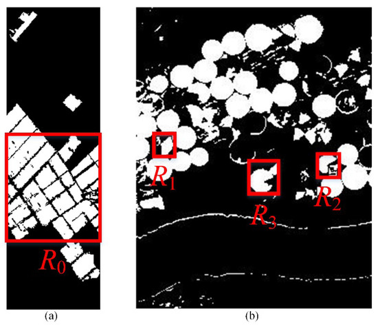
Figure 8.
Four regions are selected for analysis in detail from (a) the China dataset and (b) the USA dataset.
Figure 9 shows the change maps of all methods on the China dataset. As seen, while all methods can capture large areas, the detection details of each method are different. The detection difficulty of this dataset exists on the edges, corresponding to the subtle changes caused by the mixture of crops, bare land, and field ridges. SSCF maintains a high degree of agreement with the ground-truth map over these regions.
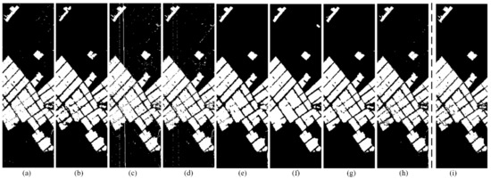
Figure 9.
Binary CM of the China dataset using different methods: (a) CVA, (b) SSIM, (c) ISFA, (d) IRMAD, (e) MaxtreeCD, (f) Unet, (g) SGCL, (h) SSCF, (i) Ground-truth.
Figure 10 shows the details of R0 with four colors, indicating four detection results. While the regions with the green and white colors are correctly detected as changed and unchanged, respectively, the areas with the pink and blue colors represent missed detections and false alarms, respectively. Obviously, SSCF has fewer missed detections and false alarms. Especially in the lower-left region, there are fewer pink and blue points relative to other methods.
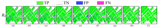
Figure 10.
Detection details of the selected region R0 on the China dataset using different methods: (a) CVA, (b) SSIM, (c) ISFA, (d) IRMAD, (e) MaxtreeCD, (f) Unet, (g) SGCL, (h) SSCF, (i) Ground-truth.
Figure 11 shows the change maps from all methods on the USA dataset. Intuitively, the change map of SSCF is closest to the ground truth. Both the large change regions and most discrete change points are detected. The false alarm rate of the ISFA method is high. The missed detection rate of the CVA, SSIM, IRMAD, and SGCL methods is high. The change map of MaxtreeCD is far away from the ground truth. Although the Unet can detect the aggregated change regions, fragmented change points are incomplete.
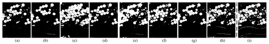
Figure 11.
Binary CM of the USA dataset using different methods: (a) CVA, (b) SSIM, (c) ISFA, (d) IRMAD, (e) MaxtreeCD, (f) Unet, (g) SGCL, (h) SSCF, (i) Ground-truth.
Figure 12 shows the details of the three selected areas (R1, R2, and R3 in Figure 8b). SSCF has the least missed detections and false alarms. Although MaxtreeCD also has fewer missed detections in these areas, the false alarms on the whole change map are higher.
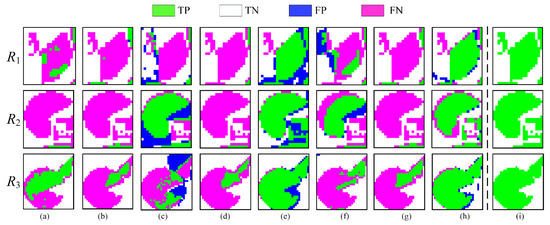
Figure 12.
Detection details of the selected regions R1, R2, and R3 on the USA dataset using different methods: (a) CVA, (b) SSIM, (c) ISFA, (d) IRMAD, (e) MaxtreeCD, (f) Unet, (g) SGCL, (h) SSCF, (i) Ground-truth.
The computation time of SSCF is compared with two deep learning methods. The computing device is equipped with Intel(R) Xeon(R) Gold 6136 CPU (2.99 GHz) and NVIDIA GeForce RTX 3090 GPU. The Unet method and the SGCL method are written in Python via the code library of PyTorch. The SSCF method does not use parallel computing. Here, we list the computing time for each dataset in Table 3. This figure shows that SSCF outperforms these two deep learning methods in terms of efficiency.
Table 3.
Time cost (seconds) of each dataset.
4. Discussion
The sensitivity of parameters needs to be analyzed. For SSCF, the selection of two parameters, the number of superpixels and the proportion of uncertain pixels, on the detection results are revealed in graphs.
Additional experiments are performed to clarify the effects of the number of superpixels parameters or the proportions of uncertain pixels on the detection results. Figure 13 shows that the influence of the number of superpixels is weak, especially for the China dataset. Furthermore, the results of SSCF at any superpixel number are more accurate than those of the comparison method. Therefore, the number of superpixels is experimentally set to 300 for better performance. It should be noted that the number of superpixels, as a parameter to be set in advance, is independent of the ground truth. For unknown data (no ground-truth available), it is recommended to choose the values in a reasonable range of 50–500, and 300 is a relatively good choice.
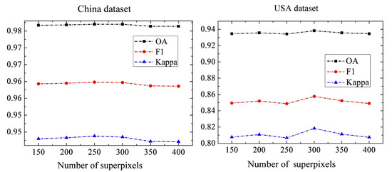
Figure 13.
SSCF experiments using different numbers of superpixels.
To evaluate the effects of randomly selecting uncertain pixels with different proportions, 10 trials with random sampling are conducted, and the average of the indexes is taken as the final result. As shown in Figure 14, the effects with different ratios are similar and steady. The lower ratio of 5% leads to a slight decrease in accuracy. To save computational resources, the ratio of 10% is preferred.
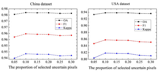
Figure 14.
SSCF experiments using different proportions of uncertain pixels.
Figure 15 shows the effect of the compactness w in SLIC on the detection performance of SSCF. Figure 16 shows the schematic diagram of the superpixel segmentation results for the two datasets based on different compactness w. The higher compactness w values lead to more complex edges. The optimal compactness of different datasets varies depending on the data characteristics. Compared with the China dataset, the USA dataset is more affected by the parameter compactness w because the spatial information is more important. As a result, a parameter of 0.6 to 1 is a good choice for both datasets. In our work, the compactness is set to 1.
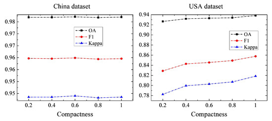
Figure 15.
SSCF experiments using different compactness w.
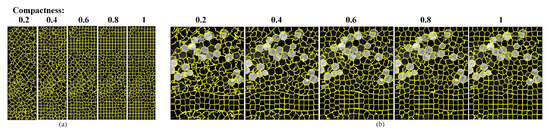
Figure 16.
Superpixel segmentation with different compactness’s on (a) the China dataset and (b) the USA dataset.
In summary, SSCF outperforms seven comparison methods with a simple and easy-to-implement framework. In particular, SSCF has a clear advantage in the simultaneous and correct detection of the subtle changes and strong changes. In addition, the robustness of the method to noise needs to be improved. The ability of SSCF to highlight subtle changes is prone to spurious changes when there is much noise in the bitemporal HSIs. Therefore, SSCF requires high preprocessing of the data.
5. Conclusions
The decision boundary of the existing HSI-CD methods is adversely affected by strong changes, which leads to the submergence of subtle changes. In this paper, SSCF is proposed to detect weak changes. SSCF treats CD as a clustering task and clusters superpixels and a randomly selected portion of uncertain pixels (rough threshold) to obtain the detection results of superpixels. In this case, the threshold is a statistical distribution independent of strong changes, so the strategy of SSCF can significantly reduce the decision boundary being adversely affected. Meanwhile, SSCF outperforms deep learning methods in terms of efficiency and outperforms other methods in terms of accuracy. It requires fewer computation resources to implement the HSI-CD task. The overall accuracy and Kappa coefficient of SSCF exceed 93% and 0.81, respectively, on the two real bitemporal HSIs datasets. The total detection time is less than 100 s. These improved detection accuracy and speed for our SSCF are important for the detection of weakly change scenes and the implementation of emergency tasks. In the future, we will combine deep learning methods with other methods to carry out HSI-CD multi-classification tasks.
Author Contributions
Conceptualization, Q.L; methodology, Q.L. and T.M.; software and experiments, Q.L. and H.G.; validation, Q.L., W.W., F.H., H.L., and A.T.; writing—original draft preparation, Q.L., X.L., Z.L., and B.W.; writing—review and editing, T.M.; funding acquisition, T.M., C.L., H.D., and Z.H. All authors contributed to the results analysis and reviewed the manuscript. All authors have read and agreed to the published version of the manuscript.
Funding
This work was supported, in part, by the National Natural Science Foundation of China (NSFC) under Grants 62175196, 61775176, and 62125505, in part, by the Shaanxi Province Key Research and Development Program under Grants 2021GXLH-Z-058, 2020GY-131, and 2021SF-135, in part, by the Innovation Capability Support Program of Shaanxi under Grant 2021TD-57, and, in part, by the Fundamental Research Funds for the Central Universities under Grant xjh012020021.
Conflicts of Interest
The authors declare no conflict of interest.
References
- Willett, R.M.; Duarte, M.F.; Davenport, M.A.; Baraniuk, R.G. Sparsity and Structure in Hyperspectral Imaging: Sensing, Reconstruction, and Target Detection. IEEE Signal Process. Mag. 2013, 31, 116–126. [Google Scholar] [CrossRef] [Green Version]
- Manolakis, D.; Marden, D.; Shaw, G.A. Hyperspectral Image Processing for Automatic Target Detection Applications. Linc. Lab. J. 2003, 14, 79–116. [Google Scholar]
- Nasrabadi, N.M. Hyperspectral Target Detection: An Overview of Current and Future Challenges. IEEE Signal Process. Mag. 2013, 31, 34–44. [Google Scholar] [CrossRef]
- Tan, K.; Hou, Z.; Wu, F.; Du, Q.; Chen, Y. Anomaly Detection for Hyperspectral Imagery Based on the Regularized Subspace Method and Collaborative Representation. Remote Sens. 2019, 11, 1318. [Google Scholar] [CrossRef] [Green Version]
- Liu, J.; Hou, Z.; Li, W.; Tao, R.; Orlando, D.; Li, H. Multipixel Anomaly Detection with Unknown Patterns for Hyperspectral Imagery. IEEE Trans. Neural Networks Learn. Syst. 2021, 2–10. [Google Scholar] [CrossRef]
- Hu, M.; Wu, C.; Zhang, L.; Du, B. Hyperspectral Anomaly Change Detection Based on Autoencoder. IEEE J. Sel. Top. Appl. Earth Obs. Remote Sens. 2021, 14, 3750–3762. [Google Scholar] [CrossRef]
- Gong, H.; Li, Q.; Li, C.; Dai, H.; He, Z.; Wang, W.; Li, H.; Han, F.; Tuniyazi, A.; Mu, T. Multiscale Information Fusion for Hyperspectral Image Classification Based on Hybrid 2D-3D CNN. Remote Sens. 2021, 13, 2268. [Google Scholar] [CrossRef]
- Zhao, Y.; Yuan, Y.; Wang, Q. Fast Spectral Clustering for Unsupervised Hyperspectral Image Classification. Remote Sens. 2019, 11, 399. [Google Scholar] [CrossRef] [Green Version]
- He, L.; Li, J.; Plaza, A.; Li, Y. Discriminative Low-Rank Gabor Filtering for Spectral–Spatial Hyperspectral Image Classification. IEEE Trans. Geosci. Remote Sens. 2016, 55, 1381–1395. [Google Scholar] [CrossRef]
- Liu, S.; Chi, M.; Zou, Y.; Samat, A.; Benediktsson, J.A.; Plaza, A.; Liu, S.; Chi, M.; Zou, Y.; Samat, A.; et al. Oil Spill Detection via Multitemporal Optical Remote Sensing Images: A Change Detection Perspective. IEEE Geosci. Remote Sens. Lett. 2017, 14, 324–328. [Google Scholar] [CrossRef]
- Bovolo, F.; Bruzzone, L. A Split-Based Approach to Unsupervised Change Detection in Large-Size Multitemporal Images: Application to Tsunami-Damage Assessment. IEEE Trans. Geosci. Remote Sens. 2007, 45, 1658–1670. [Google Scholar] [CrossRef]
- Du, P.; Liu, S.; Bruzzone, L.; Bovolo, F. Target-Driven Change Detection Based on Data Transformation and Similarity Measures. In Proceedings of the 2012 IEEE International Geoscience and Remote Sensing Symposium, Munich, Germany, 22–27 July 2012. [Google Scholar]
- Coppin, P.; Lambin, E.; Jonckheere, I.; Muys, B. Digital Change Detection Methods in Natural Ecosystem Monitoring: A Review. In Analysis of Multi-Temporal Remote Sensing Images; World Scientific: Singapore, 2002; pp. 3–36. [Google Scholar]
- Mundia, C.N.; Aniya, M. Analysis of land use/cover changes and urban expansion of Nairobi city using remote sensing and GIS. Int. J. Remote Sens. 2005, 26, 2831–2849. [Google Scholar] [CrossRef]
- Wen, D.; Huang, X.; Zhang, L.; Benediktsson, J.A. A Novel Automatic Change Detection Method for Urban High-Resolution Remotely Sensed Imagery Based on Multiindex Scene Representation. IEEE Trans. Geosci. Remote Sens. 2016, 54, 609–625. [Google Scholar] [CrossRef]
- Liu, S.; Marinelli, D.; Bruzzone, L.; Bovolo, F. A Review of Change Detection in Multitemporal Hyperspectral Images: Current Techniques, Applications, and Challenges. IEEE Geosci. Remote Sens. Mag. 2019, 7, 140–158. [Google Scholar] [CrossRef]
- Bruzzone, L.; Prieto, D. Automatic analysis of the difference image for unsupervised change detection. IEEE Trans. Geosci. Remote Sens. 2000, 38, 1171–1182. [Google Scholar] [CrossRef] [Green Version]
- Celik, T. Unsupervised Change Detection in Satellite Images Using Principal Component Analysis and k-Means Clustering. IEEE Geosci. Remote Sens. Lett. 2009, 6, 772–776. [Google Scholar] [CrossRef]
- Ertürk, A.; Iordache, M.-D.; Plaza, A. Sparse Unmixing-Based Change Detection for Multitemporal Hyperspectral Images. IEEE J. Sel. Top. Appl. Earth Obs. Remote Sens. 2016, 9, 708–719. [Google Scholar] [CrossRef]
- Dai, X.L.; Khorram, S. Remotely Sensed Change Detection Based on Artificial Neural Networks. Photogramm. Eng. Remote Sens. 1999, 65, 1187–1194. [Google Scholar]
- Singh, A. Change Detection in the Tropical Forest Environment of Northeastern India Using Landsat. In Remote Sensing and Tropical Land Management; John Wiley and Sons Ltd.: New York, NY, USA, 1986. [Google Scholar]
- Jackson, R.D. Spectral Indices in N-Space. Remote Sens. Environ. 1983, 13, 409–421. [Google Scholar] [CrossRef]
- Todd, W.J. Urban and Regional Land Use Change Detected by Using Landsat Data. J. Res. US Geol. Surv. 1977, 5, 529–534. [Google Scholar]
- Malila, W.A. Change Vector Analysis: An Approach for Detecting Forest Changes with Landsat. In Proceedings of the Sixth Annual Symposium on Machine Processing of Remotely Sensed Data and Soil Information Systems and Remote Sensing and Soil Survey, West Lafayette, IN, USA, 3–6 June 1980; pp. 326–336. [Google Scholar]
- Bovolo, F.; Marchesi, S.; Bruzzone, L. A Framework for Automatic and Unsupervised Detection of Multiple Changes in Multitemporal Images. IEEE Trans. Geosci. Remote Sens. 2012, 50, 2196–2212. [Google Scholar] [CrossRef]
- Bovolo, F.; Bruzzone, L. A Theoretical Framework for Unsupervised Change Detection Based on Change Vector Analysis in the Polar Domain. IEEE Trans. Geosci. Remote Sens. 2007, 45, 218–236. [Google Scholar] [CrossRef] [Green Version]
- Wang, Z.; Bovik, A.; Sheikh, H.; Simoncelli, E. Image Quality Assessment: From Error Visibility to Structural Similarity. IEEE Trans. Image Process. 2004, 13, 600–612. [Google Scholar] [CrossRef] [PubMed] [Green Version]
- Li, Q.; Gong, H.; Dai, H.; Li, C.; He, Z.; Wang, W.; Feng, Y.; Han, F.; Tuniyazi, A.; Li, H.; et al. Unsupervised Hyperspectral Image Change Detection via Deep Learning Self-Generated Credible Labels. IEEE J. Sel. Top. Appl. Earth Obs. Remote Sens. 2021, 14, 9012–9024. [Google Scholar] [CrossRef]
- Zhang, H.; Gong, M.; Zhang, P.; Su, L.; Shi, J. Feature-Level Change Detection Using Deep Representation and Feature Change Analysis for Multispectral Imagery. IEEE Geosci. Remote Sens. Lett. 2016, 13, 1666–1670. [Google Scholar] [CrossRef]
- Nielsen, A.A.; Conradsen, K.; Simpson, J.J. Multivariate Alteration Detection (MAD) and MAF Postprocessing in Multispectral, Bitemporal Image Data: New Approaches to Change Detection Studies. Remote Sens. Environ. 1998, 64, 1–19. [Google Scholar] [CrossRef] [Green Version]
- Frank, M.; Canty, M. Unsupervised Change Detection for Hyperspectral Images. In Proceedings of the 12th JPL Airborne Earth Science Workshop, Pasadena, CA, USA, February 2003. [Google Scholar]
- Nielsen, A.A. The Regularized Iteratively Reweighted MAD Method for Change Detection in Multi- and Hyperspectral Data. IEEE Trans. Image Process. 2007, 16, 463–478. [Google Scholar] [CrossRef] [Green Version]
- Wiskott, L.; Sejnowski, T.J. Slow Feature Analysis: Unsupervised Learning of Invariances. Neural Comput. 2002, 14, 715–770. [Google Scholar] [CrossRef]
- Wiskott, L.; Berkes, P.; Franzius, M.; Sprekeler, H.; Wilbert, N. Slow Feature Analysis. Scholarpedia 2011, 6, 5282. [Google Scholar] [CrossRef]
- Wu, C.; Zhang, L.; Du, B. Kernel Slow Feature Analysis for Scene Change Detection. IEEE Trans. Geosci. Remote Sens. 2017, 55, 2367–2384. [Google Scholar] [CrossRef]
- Wu, C.; Du, B.; Zhang, L. Slow Feature Analysis for Change Detection in Multispectral Imagery. IEEE Trans. Geosci. Remote Sens. 2014, 52, 2858–2874. [Google Scholar] [CrossRef]
- Chen, Z.; Wang, B. Spectrally-Spatially Regularized Low-Rank and Sparse Decomposition: A Novel Method for Change Detection in Multitemporal Hyperspectral Images. Remote Sens. 2017, 9, 1044. [Google Scholar] [CrossRef] [Green Version]
- Wu, C.; Du, B.; Zhang, L. Hyperspectral anomalous change detection based on joint sparse representation. ISPRS J. Photogramm. Remote Sens. 2018, 146, 137–150. [Google Scholar] [CrossRef]
- Ertürk, A. Constrained Nonnegative Matrix Factorization for Hyperspectral Change Detection. In Proceedings of the 2020 Mediterranean and Middle-East Geoscience and Remote Sensing Symposium (M2GARSS), Tunis, Tunisia, 9–11 March 2020. [Google Scholar]
- Borsoi, R.A.; Imbiriba, T.; Bermudez, J.C.M.; Richard, C. Fast Unmixing and Change Detection in Multitemporal Hyperspectral Data. IEEE Trans. Comput. Imaging 2021, 7, 975–988. [Google Scholar] [CrossRef]
- Guo, Q.; Zhang, J.; Zhang, Y. Multitemporal Hyperspectral Images Change Detection Based on Joint Unmixing and Information Coguidance Strategy. IEEE Trans. Geosci. Remote Sens. 2021, 59, 9633–9645. [Google Scholar] [CrossRef]
- Guo, Q.; Zhang, J.; Zhong, C.; Zhang, Y. Change Detection for Hyperspectral Images Via Convolutional Sparse Analysis and Temporal Spectral Unmixing. IEEE J. Sel. Top. Appl. Earth Obs. Remote Sens. 2021, 14, 4417–4426. [Google Scholar] [CrossRef]
- Seydi, S.T.; Shah-Hosseini, R.; Hasanlou, M. New framework for hyperspectral change detection based on multi-level spectral unmixing. Appl. Geomat. 2021, 13, 763–780. [Google Scholar] [CrossRef]
- Hou, Z.; Li, W.; Tao, R.; Du, Q. Three-Order Tucker Decomposition and Reconstruction Detector for Unsupervised Hyperspectral Change Detection. IEEE J. Sel. Top. Appl. Earth Obs. Remote Sens. 2021, 14, 6194–6205. [Google Scholar] [CrossRef]
- Hou, Z.; Wei, L.; Qian, D. A Patch Tensor-Based Change Detection Method for Hyperspectral Images. In Proceedings of the 2021 IEEE International Geoscience and Remote Sensing Symposium IGARSS, Brussels, Belgium, 11–16 July 2021. [Google Scholar]
- Hou, Z.; Li, W.; Li, L.; Tao, R.; Du, Q. Hyperspectral Change Detection Based on Multiple Morphological Profiles. IEEE Trans. Geosci. Remote Sens. 2021, 60, 1–12. [Google Scholar] [CrossRef]
- Chen, H.; Wu, C.; Du, B.; Zhang, L.; Wang, L. Change Detection in Multisource VHR Images via Deep Siamese Convolutional Multiple-Layers Recurrent Neural Network. IEEE Trans. Geosci. Remote Sens. 2020, 58, 2848–2864. [Google Scholar] [CrossRef]
- Peng, D.; Zhang, Y.; Guan, H. End-to-End Change Detection for High Resolution Satellite Images Using Improved UNet++. Remote Sens. 2019, 11, 1382. [Google Scholar] [CrossRef] [Green Version]
- Li, Q.; Zhong, R.; Du, X.; Du, Y. TransUNetCD: A Hybrid Transformer Network for Change Detection in Optical Remote-Sensing Images. IEEE Trans. Geosci. Remote Sens. 2022, 60, 5622519. [Google Scholar] [CrossRef]
- Shi, Q.; Liu, M.; Li, S.; Liu, X.; Wang, F.; Zhang, L. A Deeply Supervised Attention Metric-Based Network and an Open Aerial Image Dataset for Remote Sensing Change Detection. IEEE Trans. Geosci. Remote Sens. 2021, 60, 5604816. [Google Scholar] [CrossRef]
- Li, X.; Yuan, Z.; Wang, Q. Unsupervised Deep Noise Modeling for Hyperspectral Image Change Detection. Remote Sens. 2019, 11, 258. [Google Scholar] [CrossRef] [Green Version]
- Song, A.; Choi, J.; Han, Y.; Kim, Y. Change Detection in Hyperspectral Images Using Recurrent 3D Fully Convolutional Networks. Remote Sens. 2018, 10, 1827. [Google Scholar] [CrossRef] [Green Version]
- Wang, Q.; Yuan, Z.; Du, Q.; Li, X. GETNET: A General End-to-End 2-D CNN Framework for Hyperspectral Image Change Detection. IEEE Trans. Geosci. Remote Sens. 2019, 57, 3–13. [Google Scholar] [CrossRef] [Green Version]
- Du, B.; Ru, L.; Wu, C.; Zhang, L. Unsupervised Deep Slow Feature Analysis for Change Detection in Multi-Temporal Remote Sensing Images. IEEE Trans. Geosci. Remote Sens. 2019, 57, 9976–9992. [Google Scholar] [CrossRef] [Green Version]
- Sun, J.; Liu, J.; Hu, L.; Wei, Z.; Xiao, L. A Mutual Teaching Framework with Momentum Correction for Unsupervised Hyperspectral Image Change Detection. Remote Sens. 2022, 14, 1000. [Google Scholar] [CrossRef]
- Seydi, S.T.; Hasanlou, M. A New Structure for Binary and Multiple Hyperspectral Change Detection Based on Spectral Unmixing and Convolutional Neural Network. Measurement 2021, 186, 110137. [Google Scholar] [CrossRef]
- Zhou, F.; Chen, Z. Hyperspectral Image Change Detection by Self-Supervised Tensor Network. In Proceedings of the IGARSS 2020–2020 IEEE International Geoscience and Remote Sensing Symposium, Waikoloa, HI, USA, 26 September–2 October 2020. [Google Scholar]
- Saha, S.; Kondmann, L.; Zhu, X.X. Deep no learning approach for unsupervised change detection in hyperspectral images. ISPRS Ann. Photogramm. Remote Sens. Spat. Inf. Sci. 2021, 3, 311–316. [Google Scholar] [CrossRef]
- Lei, J.; Li, M.; Xie, W.; Li, Y.; Jia, X. Spectral mapping with adversarial learning for unsupervised hyperspectral change detection. Neurocomputing 2021, 465, 71–83. [Google Scholar] [CrossRef]
- Hasanlou, M.; Seydi, S.T. Hyperspectral change detection: An experimental comparative study. Int. J. Remote Sens. 2018, 39, 7029–7083. [Google Scholar] [CrossRef]
- Achanta, R.; Shaji, A.; Smith, K.; Lucchi, A.; Fua, P.; Süsstrunk, S. SLIC Superpixels Compared to State-of-the-Art Superpixel Methods. IEEE Trans. Pattern Anal. Mach. Intell. 2012, 34, 2274–2282. [Google Scholar] [CrossRef] [Green Version]
- Friedman, N.; Russell, S. Image Segmentation in Video Sequences: A Probabilistic Approach. arXiv 2013, arXiv:1302.1539. [Google Scholar]
- Datt, B.; McVicar, T.; Van Niel, T.; Jupp, D.; Pearlman, J. Preprocessing eo-1 hyperion hyperspectral data to support the application of agricultural indexes. IEEE Trans. Geosci. Remote Sens. 2003, 41, 1246–1259. [Google Scholar] [CrossRef] [Green Version]
- Folkman, M.; Pearlman, J.; Liao, L.; Jarecke, P. Eo-1/Hyperion Hyperspectral Imager Design, Development, Characterization, and Calibration. Proc. SPIE 2001, 4151, 40–51. [Google Scholar]
- Pearlman, J.; Barry, P.; Segal, C.; Shepanski, J.; Beiso, D.; Carman, S. Hyperion, a space-based imaging spectrometer. IEEE Trans. Geosci. Remote Sens. 2003, 41, 1160–1173. [Google Scholar] [CrossRef]
- Yuan, Y.; Lv, H.; Lu, X. Semi-supervised change detection method for multi-temporal hyperspectral images. Neurocomputing 2015, 148, 363–375. [Google Scholar] [CrossRef]
- Ronneberger, O.; Fischer, P.; Brox, T. U-Net: Convolutional Networks for Biomedical Image Segmentation. In Proceedings of the International Conference on Medical Image Computing and Computer-Assisted Intervention, Munich, Germany, 5–9 October 2015. [Google Scholar]
Publisher’s Note: MDPI stays neutral with regard to jurisdictional claims in published maps and institutional affiliations. |
© 2022 by the authors. Licensee MDPI, Basel, Switzerland. This article is an open access article distributed under the terms and conditions of the Creative Commons Attribution (CC BY) license (https://creativecommons.org/licenses/by/4.0/).