
Remote Sensing Analysis of Ecological Maintenance in Subtropical Coastal Mountain Area, China

 ,
, 

Abstract
:
1. Introduction
2. Materials and Methods
2.1. Survey and Data Sources of Study Areas
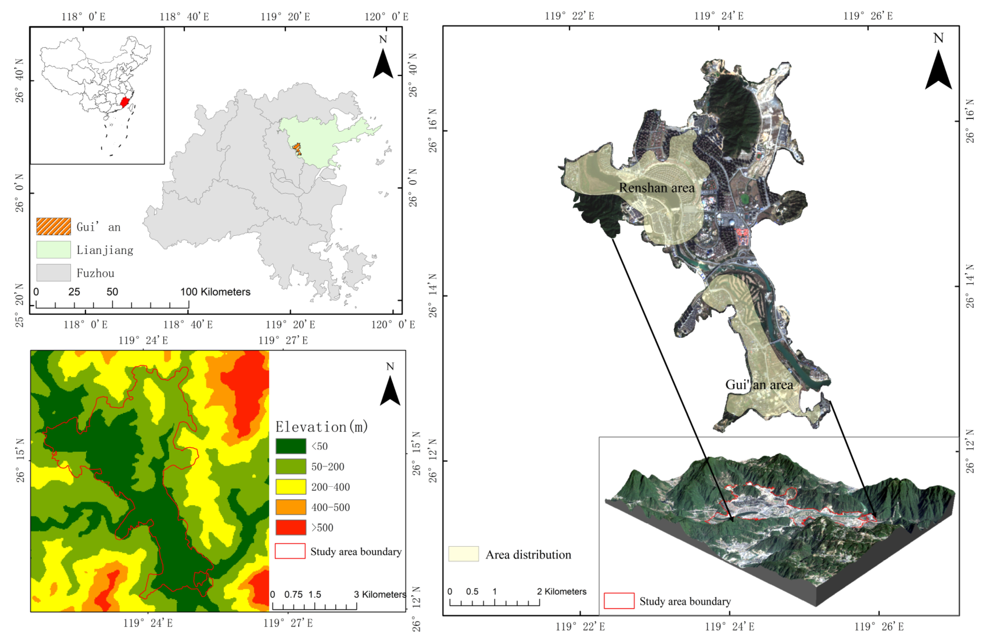
2.1.1. Study Area
2.1.2. Data Sources and Pre-Processing
2.2. Research Methods
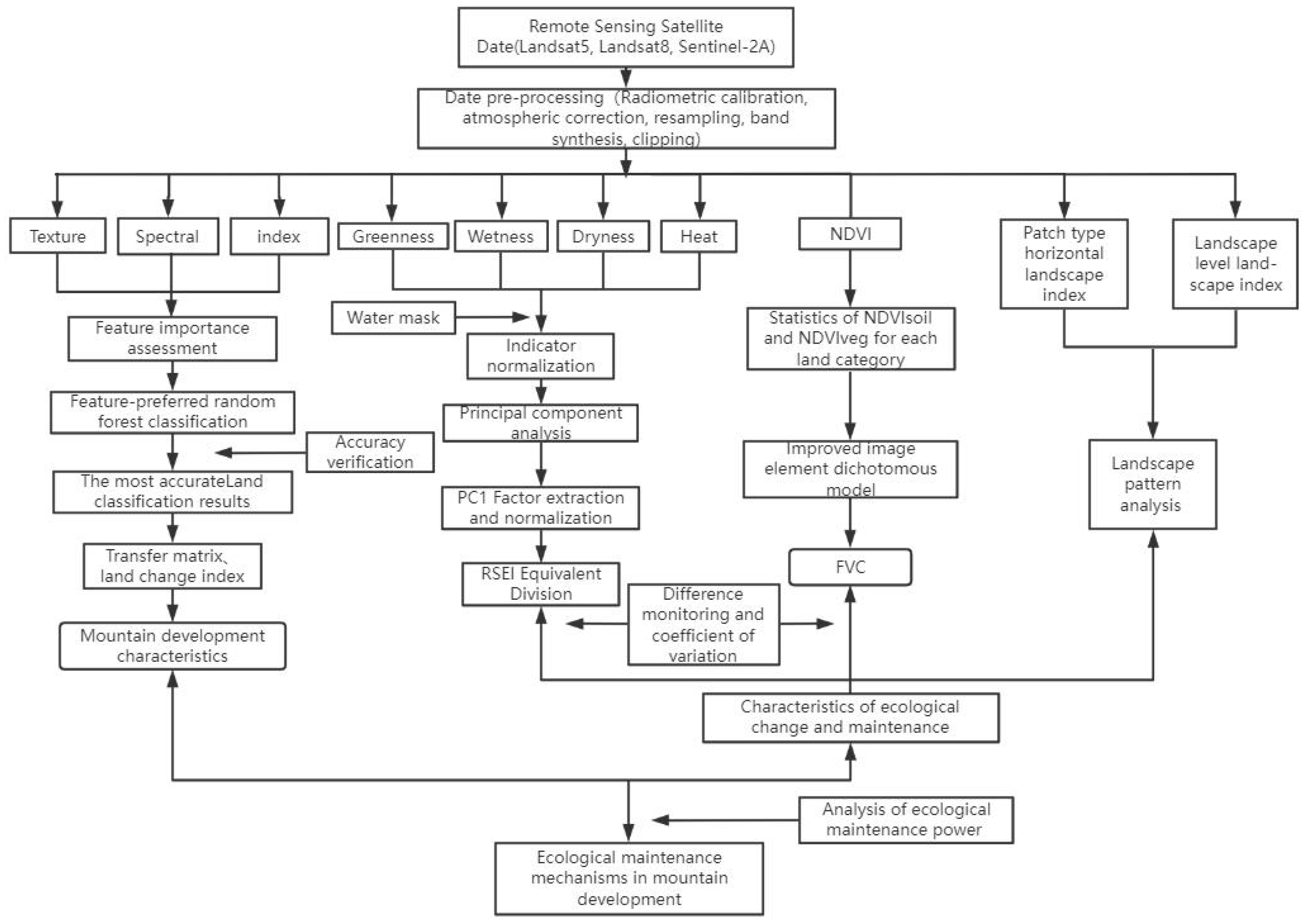
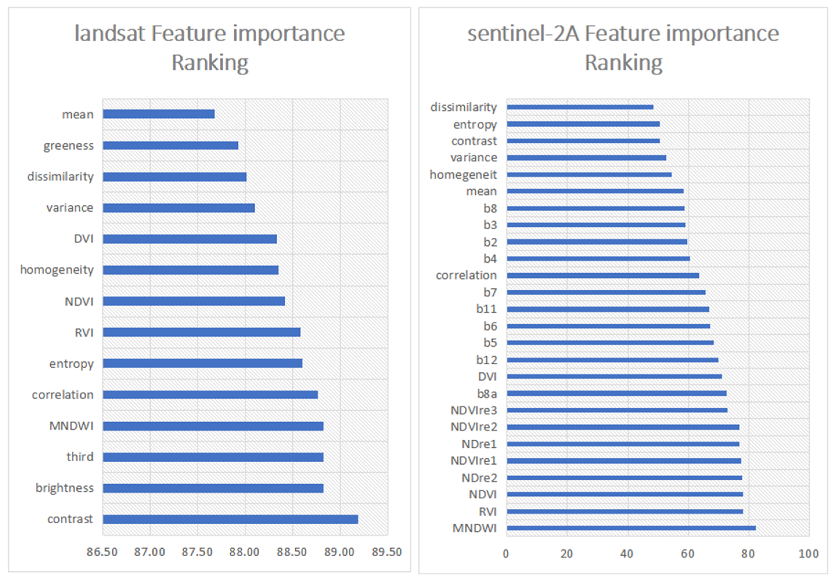
2.2.1. Optimization of Random Forest Classification
2.2.2. Land-Use Change Index
2.2.3. Analysis of the Transfer Matrix
2.2.4. Landscape Pattern Index
2.2.5. Remote Sensing Ecological Index Model
- (1)
- Greenness index (NDVI)
- (2)
- Humidity index (Wet)
- (3)
- Dryness index
- (4)
- Heat index (LST)
2.2.6. Fractional Vegetation Cover
2.2.7. Coefficient of Variation
2.2.8. Difference Calculation
3. Results
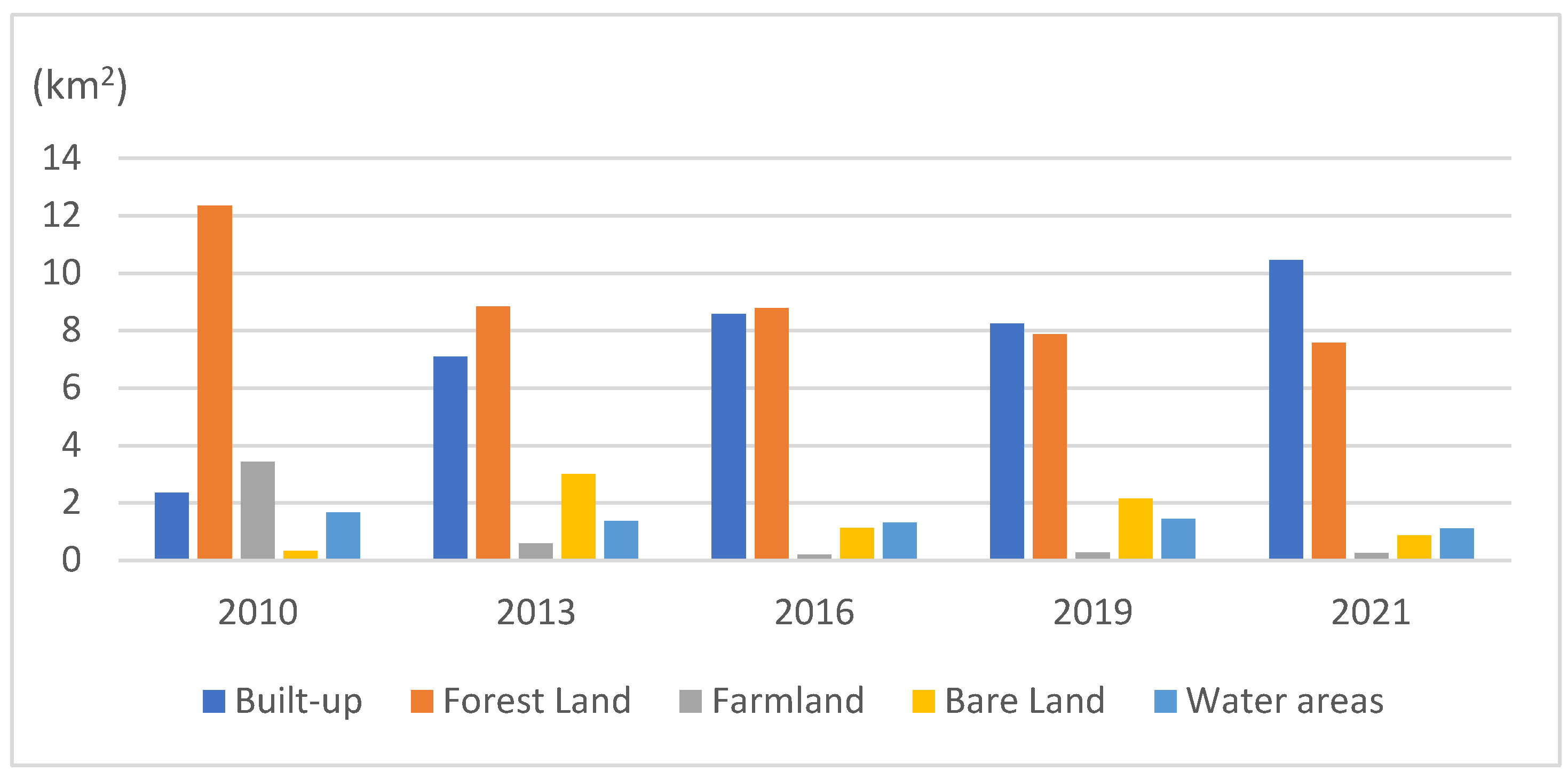
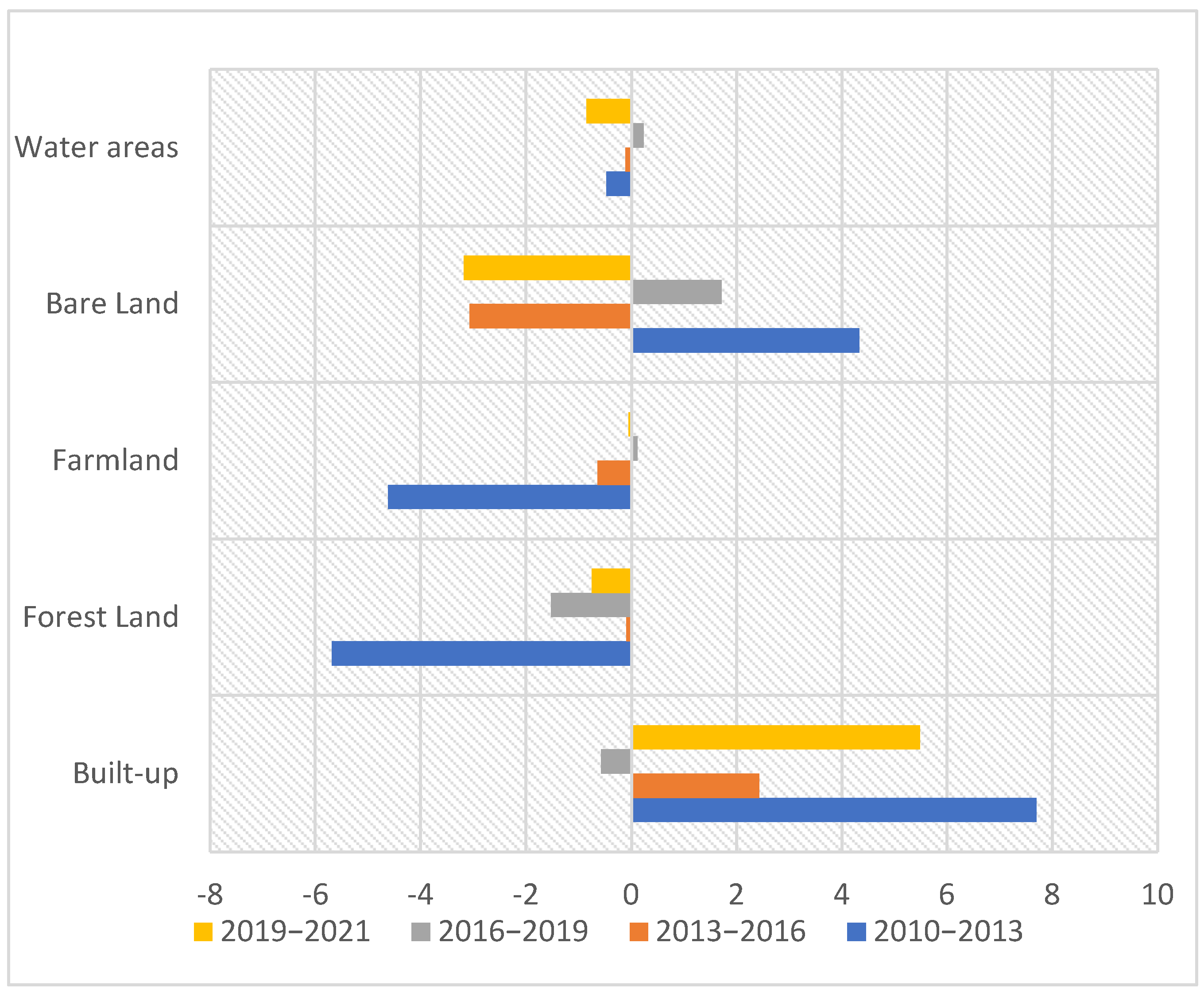
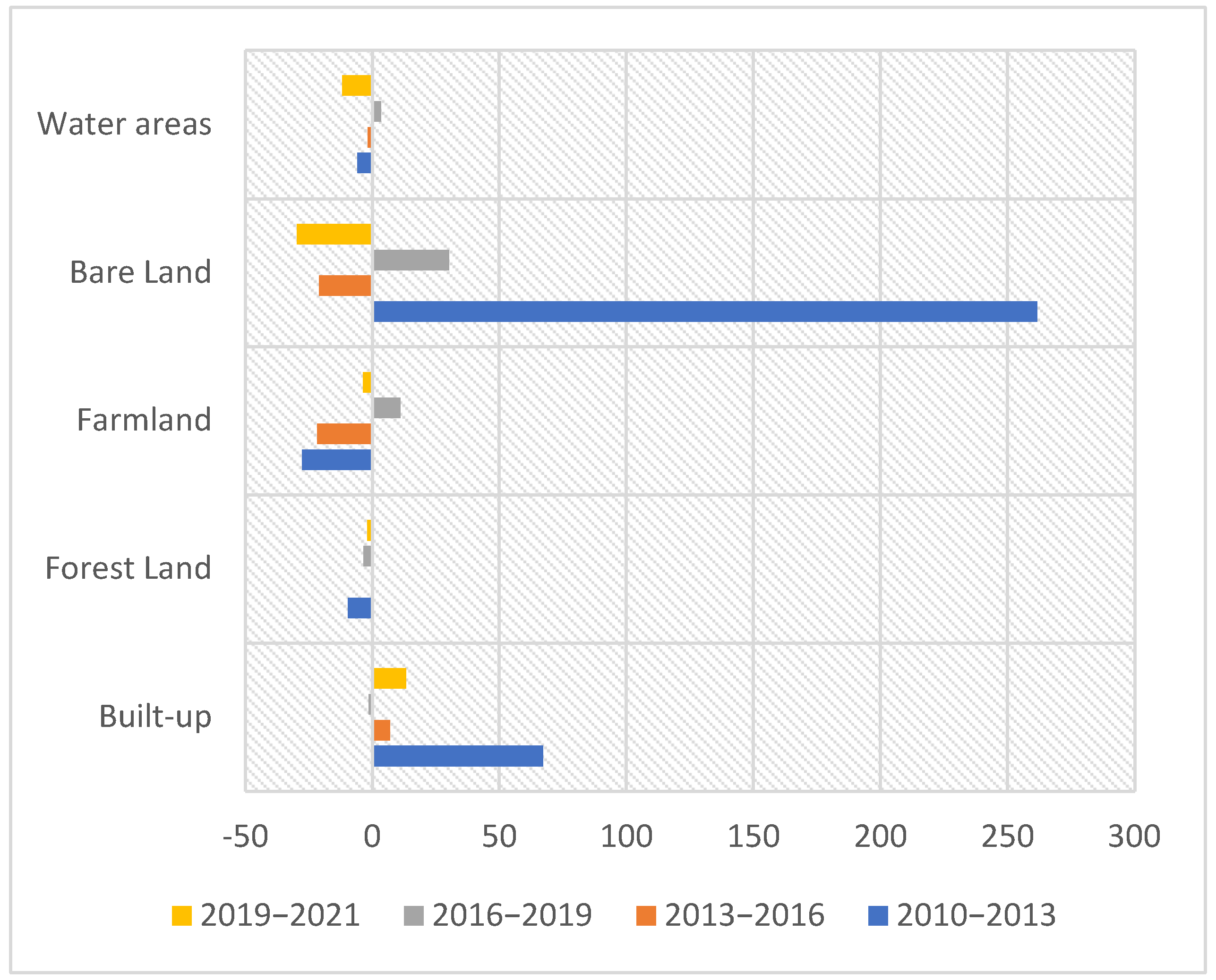
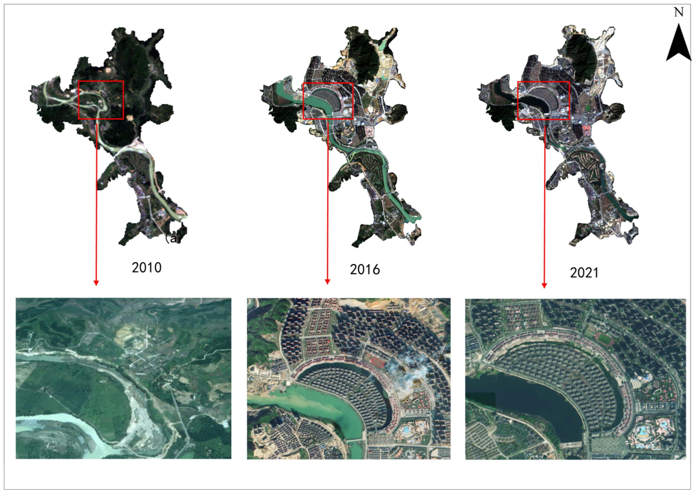
3.1. Characteristics of Mountain Development Pattern
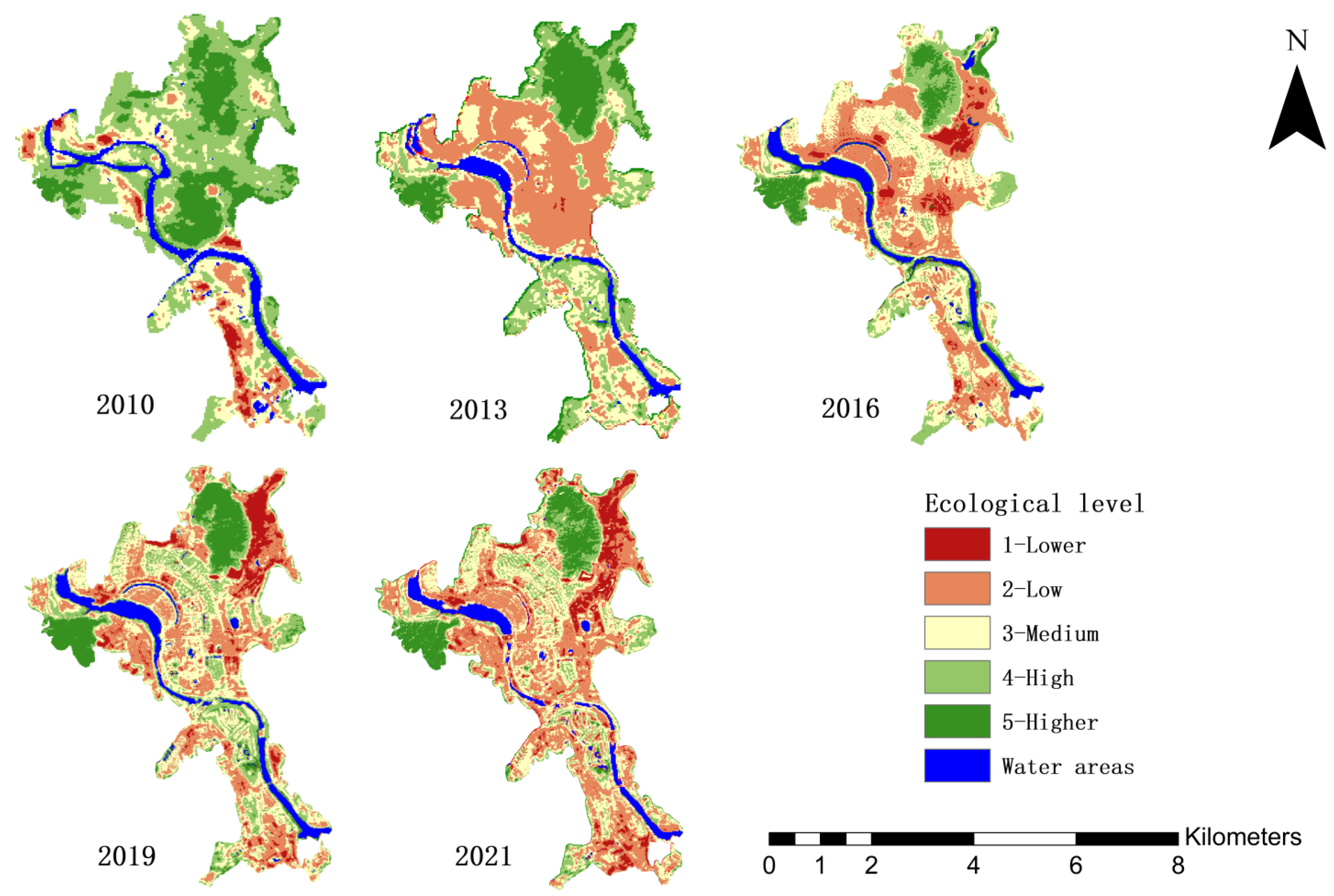
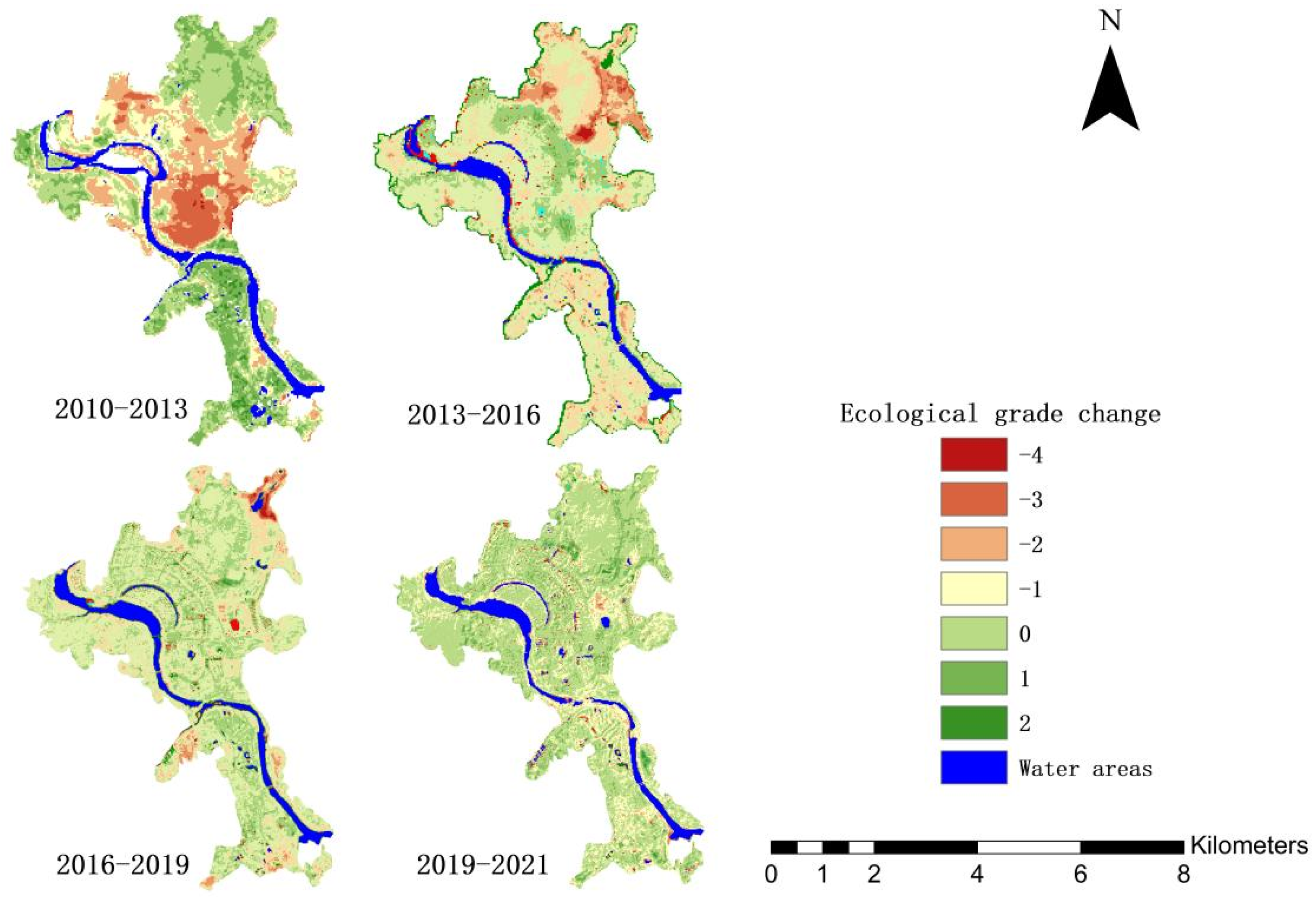
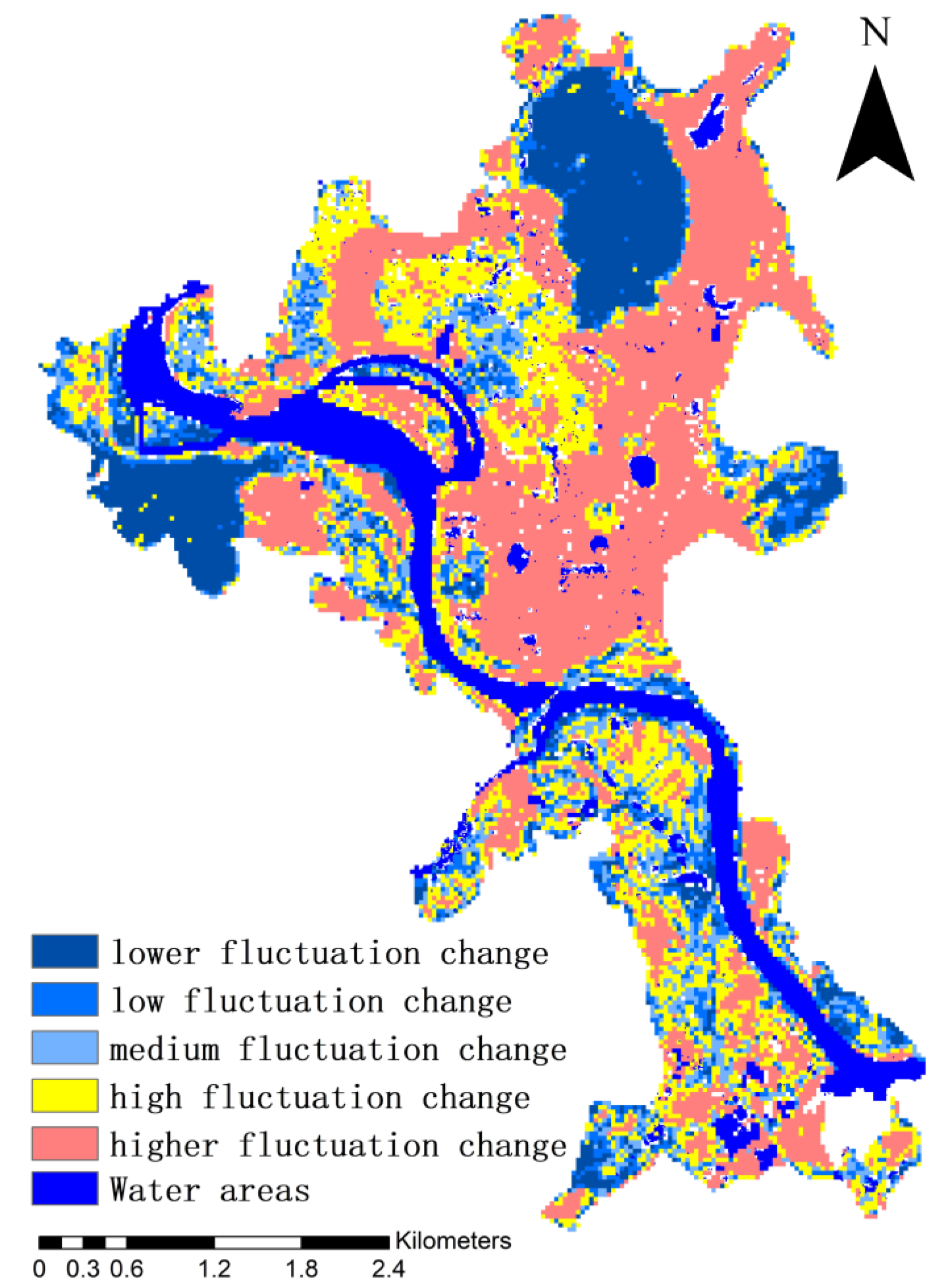
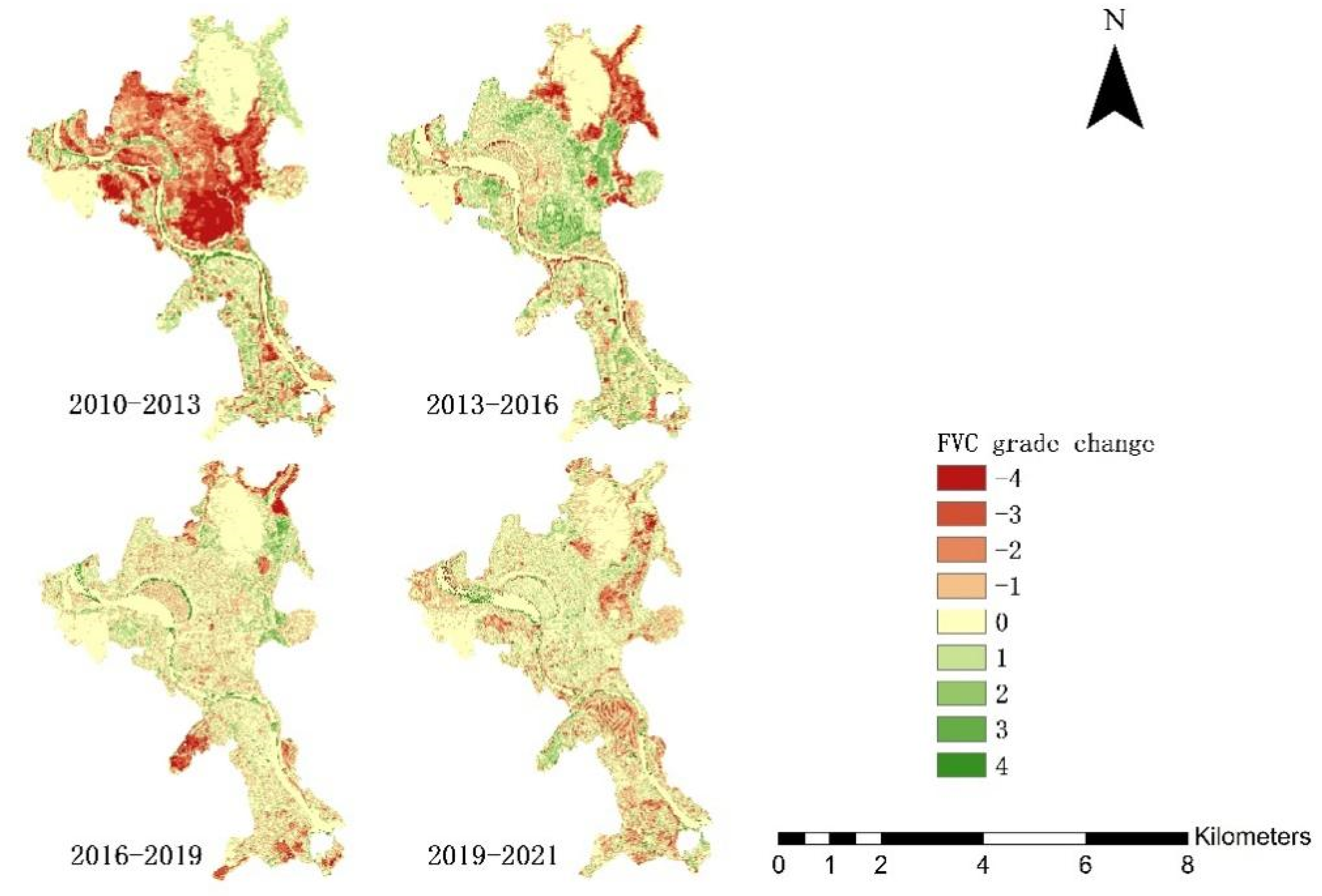
3.2. Analysis of Spatial and Temporal Changes in Ecological Maintenance
4. Discussion
5. Conclusions
Author Contributions
Funding
Data Availability Statement
Acknowledgments
Conflicts of Interest
References
- Holdren, J.P.; Ehrlich, P.R. Human population and the global environment. Am. Sci. 1974, 62, 282–297. [Google Scholar]
- Ehrlich, P.R.; Ehrlich, A.H. The value of biodiversity. Ambio 1992, 21, 219–226. [Google Scholar]
- Zhang, X.; Li, Y.; Lu, C.; BI, R.; Xia, L.; Guo, Y.; Wang, Y.; Xu, C.; Sun, B. Ecosystem services based on InVEST model. Appl. Res. Prog. Ecol. Sci. 2022, 41, 237–242. [Google Scholar]
- Sun, H.; Hu, J.; Cui, Y.; Yang, N.; Cai, C. Spatial-temporal evolution trend analysis of ecosystem services based on multi-source remote sensing data. Bull. Surv. Mapp. 2021, 4, 1–7. [Google Scholar]
- Li, A.N.; Wang, A.S.; Liang, S.L.; Zhou, W.C. Eco-environmental vulnerability evaluation in mountainous region using remote sensing and GIS-A case study in the upper reaches of Minjiang River, China. Ecol. Model. 2006, 192, 175–187. [Google Scholar] [CrossRef]
- Liao, K. Mapping method of eco-environmental remote sensing complex series. Acta Geogr. Sin. 2005, 60, 479–486. [Google Scholar]
- Li, A.; Bian, J.; Zhang, Z.; Zhao, W.; Yin, G. Research progress, opportunities and challenges of mountain remote sensing. J. Remote Sens. 2016, 20, 1199–1215. [Google Scholar]
- Bian, J.H.; Li, A.N.; Song, M.Q.; Ma, L.Q.; Jiang, J.G. Reconstruction of NDVI time-series datasets of MODIS based on Savitzky Golay filter. J. Remote Sens. 2010, 14, 725–741. [Google Scholar]
- Feng, Y.; Cao, Y.; Li, S.; Wang, S.; Liu, S.; Bai, Z. Ecosystem services tradeoffs and collaborative research, development and research characteristics. J. Agric. Resour. Environ. 2022, 33, 11–25. [Google Scholar]
- Zhang, S.; Liu, R.; Hou, H.; Yang, Y. Research progress in ecological restoration monitoring: A statistical analysis based on the reports of the last three World Congress on Ecological Restoration. Chin. J. Ecol. 2018, 37, 1605–1611. [Google Scholar]
- Fu, B. National spatial ecological restoration to grasp the main points. Proc. Chin. Acad. Sci. 2021, 4, 64–69. [Google Scholar]
- Cao, Y.; Wang, J.; Li, G.-Y. Concept of national spatial ecological restoration: Speculative and cognitive theory. J. China Land Sci. 2019, 7, 1–10. [Google Scholar]
- UN. Transforming Our World: The 2030 Agenda for Sustainable Development; United Nations: New York, NY, USA, 2015.
- Zhang, H.; LI, Z.; Li, Y. Study on sustainable land use pattern in mountain towns based on ecological security: A case study of Dali City, Yunnan Province. Geogr. Res. 2019, 38, 2681–2694. [Google Scholar]
- Meyfroidt, P.; de Bremond, A.; Ryan, C.M.; Archer, E.; Aspinall, R.; Chhabra, A.; Camara, G.; Corbera, E.; DeFries, R.; Díaz, S.; et al. Ten facts about land systems for sustainability. Proc. Natl. Acad. Sci. USA 2022, 119, e2109217118. [Google Scholar] [CrossRef]
- Ding, Y.; Zhang, L.; Wu, Y. The dilemma and way out of mountain urbanization: Taking Dali Prefecture in Yunnan Province as an example. J. Mt. Land 2018, 36, 917–929. [Google Scholar]
- Gu, X.-T.; Gao, X.-H.; Ma, H.-J.; Shi, F.-F.; Liu, X.-M.; Cao, X.-M. Comparison of machine learning methods for land use/land cover classification in complex terrain areas. Remote Sens. Technol. Appl. 2019, 34, 57–67. [Google Scholar]
- Zhao, D.; Gu, H.; Jia, Y. Comparision of Machine Learning Method in Object-based Image Classification. Sci. Surv. Mapp. 2016, 41, 181–186. [Google Scholar] [CrossRef]
- Li, M.; Wang, M.; Wang, F.; Chen, X.; Ding, W. Urban land use classification by multi-featured random forest. Mapp. Sci. 2022, 6, 1–8. Available online: http://kns.cnki.net/kcms/detail/11.4415.P.20210923.0819.004.html (accessed on 30 May 2022).
- Li, Q.; Shi, M.W. A study on multi-temporal Landsat8 land use classification based on random forest. Inf. Technol. Informatiz. 2019, 7, 181–183. [Google Scholar]
- Ma, H.; Gao, X.; Gu, X. A study on land use/land cover classification in complex terrain areas supported by random forest method. J. Geoinf. Sci. 2019, 21, 359–371. [Google Scholar]
- Zhang, X.; Li, F.; Zhen, Z.; Zhao, Y. Forest vegetation classification using Landsat 8 remote sensing images based on random forest model. J. Northeast. For. Univ. 2016, 44, 53–57. [Google Scholar]
- Gong, P. Vegetation classification based on phenology indices derived from MO-DIS Data in Northeastern China. Resour. Sci. 2010, 32, 1154–1160. [Google Scholar]
- Chen, W.Q.; Ding, J.L.; Li, Y.H.; Niu, Z.Y. Extraction of water information based on China-made GF-1 remote sense image. Resour. Sci. 2015, 37, 1166–1172. [Google Scholar]
- Li, Z.; Zhu, G.; Dong, T. Image texture feature classification based on gray co-occurrence matrix. Geol. Explor. 2011, 47, 456–461. [Google Scholar]
- Hu, Y.-F.; Deng, L.-J.; Kuang, X.-H.; Wang, P.; He, S.; Xiong, L. Land use classification based on texture features in high-resolution remote sensing images. Geogr. Geo-Inf. Sci. 2011, 27, 42–45. [Google Scholar]
- He, Y.; Huang, C.; Li, H.; Liu, Q.S.; Liu, G.h.; Zhou, Z.C.; Zhang, C.C. Random forest land cover classification based on Sentinel-2A image feature preference. Resour. Sci. 2019, 41, 992–1001. [Google Scholar]
- Zhang, H.H.; Zhao, W.C.; Liu, Q.K. Feature-preferred random forest for land use classification. J. Heilongjiang Univ. Sci. Technol. 2020, 30, 490–494. [Google Scholar]
- Zhang, L.; Gong, Z.; Wang, Q.; Jin, D.; Wang, X. Extraction of wetland information from Sentinel-2 image based on multi-feature optimization. J. Remote Sens. 2019, 23, 313–326. [Google Scholar]
- Zhan, G.Q.; Yang, G.D.; Wang, F.Y.; Xin, X.W.; Guo, C.; Zhao, Q. Research on random forest algorithm based on feature space optimization in GF-2 image wetland classification. J. Geoinf. Sci. 2018, 20, 1520–1528. [Google Scholar]
- Fang, J.; Sha, J.; Zhou, Z.; Lin, Q. Random forest based land use change and urban driven analysis. Comput. Syst. Appl. 2021, 30, 12–20. [Google Scholar]
- Sun, Y.; Zhao, S.Q.; Qu, W.Y. Quantifying spatiotemporal patterns of urban expansion in three capital cities in Northeast China over the past three decades. Environ. Earth Sci. 2015, 73, 7221–7235. [Google Scholar] [CrossRef]
- Wu, B.; Ci, L. Study on the change of landscape pattern in Mawusu Sandy. J. Ecol. 2001, 21, 191–196. [Google Scholar]
- Liang, X.; Gu, Z.; Lei, M.; Wang, X. A Study on the Differences between Land Function and Land Use Characterization Land System and Landscape Pattern-Shaanxi. A Case Study of Lantian County, Shanxi province. J. Nat. Resour. 2014, 29, 1127–1135. [Google Scholar]
- Pang, B.; Chen, D.; Li, W.; Wang, Y.L. Study on the stability of land use landscape pattern with the example of Changde City. Geoscience 2013, 33, 1484–1488. [Google Scholar]
- Svoray, T.; Bar, P.; Bannet, T. Urban land-use allocation in a Mediterranean ecotone: Habitat heterogeneity model incorporated in a GIS using a multi-criteria mechanism. Landsc. Urban Plan. 2005, 72, 337–351. [Google Scholar] [CrossRef]
- Buyantuyev, A.; Wu, J.; Gries, C. Multiscale analysis of the urbanization pattern of the Phoenix metropolitan landscape of USA: Time, space and thematic resolution. Landsc. Urban Plan. 2015, 94, 206–217. [Google Scholar] [CrossRef]
- Xu, H. The creation of urban remote sensing ecological index and its application. J. Ecol. 2013, 33, 7853–7862. [Google Scholar]
- Xu, H. Remote sensing evaluation index of regional ecological environment change. China Environ. Sci. 2013, 33, 889–897. [Google Scholar]
- Yang, H.; Xu, H. Vegetation coverage change and ecological quality assessment in Wuyi Mountain National Nature Reserve based on remote sensing spatial information. Chin. J. Appl. Ecol. 2020, 31, 533–542. [Google Scholar]
- Li, T.; Ma, C.; Guo, C. Evaluation and influencing factors of ecological quality in Helan Mountain based on RSEI model. Chin. J. Ecol. 2021, 40, 1154–1165. [Google Scholar] [CrossRef]
- Crist, E.P. A TM tasseled cap equivalent transformation for reflectance factor data. Remote Sens. Environ. 1985, 17, 301–306. [Google Scholar] [CrossRef]
- Li, B.; Lun, X.; Chao, P.; Yan, X. Derivation of tasseled cap transformation for Landsat 8 land imager images. Surv. Mapp. Sci. 2016, 41, 102–107. [Google Scholar]
- Roy, P.S.; Rikimaru, A.; Miyatake, S. Tropical forest cover density mapping. Trop. Ecol. 2002, 43, 39–47. [Google Scholar]
- Hu, D.Y.; Qiao, K.; Wang, X.L.; Zhao, L.; Ji, G. Single-window algorithm for inversion of surface temperature with Landsat8 thermal infrared data. J. Remote Sens. 2015, 19, 964–976. [Google Scholar]
- Jin, D.; Gong, Z. Comparative analysis of surface temperature inversion algorithms based on Landsat series data—Take Qiqihar city district as an example. Remote Sens. Technol. Appl. 2018, 33, 830–841. [Google Scholar]
- Zhang, F.; Guo, Y. Surface temperature inversion of Landsat imagery and its intensity variation analysis. Mapp. Sci. 2020, 45, 61–66+94. [Google Scholar]
- Kutiel, P.; Cohen, O.; Shoshany, M.; Shub, M. Vegetation establishment on the southern Israeli coastal sand dunes between the years 1965 and 1999. Landsc. Urban Plan. 2004, 67, 141–156. [Google Scholar] [CrossRef]
- Gan, C.-Y.; Wang, R.; Li, B.; Liang, Z.-X.; Li, Z.-W.; Wen, X.-H. Analysis of vegetation cover changes in the Lianjiang River Basin over the past 18 years. Geoscience 2011, 31, 1019–1024. [Google Scholar]
- Li, M.; Wu, B.; Yan, C.; Zhou, W.F. Remote sensing estimation of vegetation cover in the upper reaches of Miyun Reservoir. Resour. Sci. 2004, 26, 153–159. [Google Scholar]
- Zhang, S.; Zhang, R.; Liu, T.; Xu, R.; Zhang, P. Analysis of spatial and temporal dynamics and influencing factors of vegetation cover in Xilingole grassland. J. Agric. Mach. 2017, 48, 253–260. [Google Scholar]
- Xiong, J.; Peng, C.; Cheng, W.; Li, W.; Liu, Z.; Fan, C.; Sun, H. Analysis of vegetation cover change in Yunnan Province based on MODIS-NDVI. J. Geoinf. Sci. 2018, 20, 1830–1840. [Google Scholar]
- Wang, G.; Bi, R.; Zhang, W.P.; Zhang, X.J.; Yao, D. Spatial and temporal distribution characteristics and influencing factors of vegetation cover in typical mining areas. J. Ecol. 2020, 40, 6046–6056. [Google Scholar]
- Huang, Y.; Yang, D.; Feng, L. Spatial and temporal variation of vegetation cover and its drivers in Ningxia from 2000–2016. J. Ecol. 2019, 38, 2515–2523. [Google Scholar]
- Zhang, S.; Zhao, H.; Zhang, F.; Shang, S. Spatial and temporal dynamics of Xilinguole grassland based on MODIS NDVI in the past 10 years. Grassl. Sci. 2014, 31, 1416–1423. [Google Scholar]
- Nong, L.; Wang, J.; Yu, Y. Research on ecological environment quality in central Yunnan based on the improved remote sensing ecological index (MRSEI) model. J. Ecol. Rural Environ. 2021, 37, 972–982. [Google Scholar]
- Wang, Q.; Zhao, W.; Zhang, Y. Research on ecological environment changes in the Songnen Plain based on FVC index. Mapp. Spat. Geogr. Inf. 2021, 44, 164–167. [Google Scholar]
- Hu, S.; Yao, Y.; Fu, J.; Zhao, J.; Hao, D. Evaluation of ecological quality changes in mining areas in Northeast China based on RSEI index: An example from Gongchangling District, Liaoning. J. Ecol. 2021, 40, 4053–4060. [Google Scholar] [CrossRef]
- Li, X.; Yin, J.; Li, X. Research on the development model of mountain ecotourism in western region based on spatio-temporal three-dimensional perspective. Ecol. Econ. 2011, 7, 124–127. [Google Scholar]


| The Data Type | Image Time | Row Number | Spatial Resolution |
|---|---|---|---|
| Landsat 5 | 24 May 2010 | 119/042 | 30 m |
| Landsat 8 | 4 August 2013 | ||
| Sentinel-2A | 25 January 2016 | 10 m | |
| 29 January 2019 | |||
| 18 January 2021 | |||
| DEM | 2009 | 30 m |
| Feature Type | Feature Variable | Abbreviation | Description |
|---|---|---|---|
| Spectral | Band | Band | b2, b3, b4, b5, b6, b7, b8, b8a, b11, b12 |
| Vegetation index | Normalized Difference Vegetation Index | NDVI | (b8 − b4)/(b8 + b4) |
| Ratio Vegetation Index | RVI | b8/b4 | |
| Difference Vegetation Index | DVI | b8 − b4 | |
| Water index | Modified Normalized Difference Water Index | MNDWI | (b3 − b11)/(b3 + b11) |
| Red edge index | Normalized Difference Vegetation Index1 | NDVIre1 | (b8a − b5)/(b8a + b5) |
| Normalized Difference Vegetation Index2 | NDVIre2 | (b8a − b6)/(b8a + b6) | |
| Normalized Difference Vegetation Index3 | NDVIre3 | (b8a − b7)/(b8a + b7) | |
| Normalized Difference 1 | NDre1 | (b6 − b5)/(b6 + b5) | |
| Normalized Difference2 | NDre2 | (b7 − b5)/(b7 + b5) | |
| Texture | Mean | Mean | - |
| Variance | Variance | - | |
| Contrast | Contrast | - | |
| Entropy | Entropy | - | |
| Correlation | Correlation | - | |
| Homogeneity | Homogeneity | - | |
| Dissimilarity | Dissimilarity | - |
| Feature Type | Feature Variable | Abbreviation | Description |
|---|---|---|---|
| Vegetation index | Normalized Difference Vegetation Index | NDVI | (NIR − R)/(NIR + R) |
| Ratio Vegetation Index | RVI | NIR/R | |
| Difference Vegetation Index | DVI | NIR − R | |
| Water index | Modified Normalized Difference Water Index | MNDWI | (Green − MIR)/(Green + MIR) |
| Texture | Mean | Mean | - |
| Variance | Variance | - | |
| Contrast | Contrast | - | |
| Entropy | Entropy | - | |
| Correlation | Correlation | - | |
| Homogeneity | Homogeneity | - | |
| Dissimilarity | Dissimilarity | - | |
| Tassel cap change | Brightness | Brightness | - |
| Greenness | Greenness | - | |
| Wetness | Wetness | - |
| Image Data Type | Scheme | Number of Features | Kappa% |
|---|---|---|---|
| Sentinel-2A | 1 | 6 | 89.53 |
| 2 | 10 | 90.16 | |
| 3 | 14 | 89.61 | |
| 4 | 20 | 89.56 | |
| 5 | 26 | 89.31 | |
| Landsat | 1 | 5 | 90.11 |
| 2 | 10 | 88.85 | |
| 3 | 14 | 89.35 |
| Year (Latter\Early) | Built-Up | Water Areas | Bare Land | Farmland | Forest Land | |
|---|---|---|---|---|---|---|
| Built-up | 71.89 | 25.20 | 74.41 | 43.47 | 25.94 | |
| Water areas | 4.10 | 53.75 | 2.61 | 3.35 | 1.93 | |
| 2010–2013 | Bare land | 6.40 | 1.67 | 13.58 | 17.71 | 17.61 |
| Farmland | 2.57 | 2.16 | 1.57 | 5.89 | 2.31 | |
| Forest land | 15.05 | 17.22 | 7.83 | 29.58 | 52.23 | |
| 2013–2016 | Built-up | 65.69 | 4.96 | 76.53 | 24.33 | 14.65 |
| Water areas | 1.45 | 76.58 | 0.72 | 1.94 | 1.35 | |
| Bare land | 4.35 | 0 | 7.46 | 8.51 | 6.63 | |
| Farmland | 0.61 | 0.13 | 0.36 | 9.41 | 0.90 | |
| Forest land | 26.39 | 16.12 | 14.58 | 50.60 | 66.55 | |
| Built-up | 72.74 | 5.98 | 36.34 | 10.00 | 17.01 | |
| Water areas | 1.29 | 84.98 | 1.01 | 1.74 | 2.37 | |
| 2016–2019 | Bare land | 10.52 | 4.52 | 50.04 | 8.55 | 7.02 |
| Farmland | 0.91 | 0.66 | 3.16 | 14.73 | 1.46 | |
| Forest land | 14.54 | 3.86 | 9.45 | 64.98 | 72.14 | |
| 2019–2021 | Built-up | 89.48 | 29.34 | 50.64 | 37.03 | 17.74 |
| Water areas | 0.61 | 68.72 | 0.19 | 3.42 | 0.62 | |
| Bare land | 1.92 | 1.06 | 27.58 | 4.13 | 1.22 | |
| Farmland | 0.35 | 0.01 | 0.30 | 12.56 | 2.37 | |
| Forest land | 7.64 | 0.86 | 21.29 | 42.87 | 78.05 |
| RSEI Level | 2010 | 2013 | 2016 | 2019 | 2021 | |||||
|---|---|---|---|---|---|---|---|---|---|---|
| Area km2 | Scale% | Area km2 | Scale% | Area km2 | Scale% | Area km2 | Scale% | Area km2 | Scale% | |
| Lower | 0.45 | 2.45 | 0.0675 | 0.36 | 0.7122 | 3.92 | 1.3607 | 7.34 | 1.5738 | 8.44 |
| Low | 1.8459 | 10.05 | 6.9192 | 36.66 | 6.5334 | 35.96 | 5.5576 | 29.97 | 6.903 | 37.03 |
| Medium | 4.0671 | 22.15 | 4.923 | 26.08 | 6.4388 | 35.44 | 5.8897 | 31.76 | 6.036 | 32.38 |
| High | 7.9434 | 43.25 | 4.2039 | 22.27 | 3.0807 | 16.96 | 3.6833 | 19.86 | 2.408 | 12.92 |
| Higher | 4.059 | 22.10 | 2.7603 | 14.62 | 1.4022 | 7.72 | 2.0511 | 11.06 | 1.723 | 9.24 |
| Category | Level Difference | Level Area | Class Area | Scale% | |
|---|---|---|---|---|---|
| 2010–2013 | Falling | −4 | 0.0279 | 8.2026 | 45.64 |
| −3 | 1.4778 | ||||
| −2 | 3.1833 | ||||
| −1 | 3.5136 | ||||
| Unchanged | 0 | 6.084 | 6.084 | 33.85 | |
| Rising | 1 | 3.4515 | 3.6864 | 20.51 | |
| 2 | 0.2349 | ||||
| 3 | — | ||||
| 2013–2016 | Falling | −4 | 0.054 | 6.3216 | 35.04 |
| −3 | 0.2916 | ||||
| −2 | 1.2357 | ||||
| −1 | 4.7403 | ||||
| Unchanged | 0 | 8.4456 | 8.4456 | 46.82 | |
| Rising | 1 | 2.9619 | 3.2724 | 18.14 | |
| 2 | 0.3015 | ||||
| 3 | 0.009 | ||||
| 2016–2019 | Falling | −4 | 0.0444 | 2.9669 | 16.48 |
| −3 | 0.1089 | ||||
| −2 | 0.4288 | ||||
| −1 | 2.3848 | ||||
| Unchanged | 0 | 10.0074 | 10.0074 | 55.58 | |
| Rising | 1 | 4.819 | 5.0312 | 27.94 | |
| 2 | 0.2003 | ||||
| 3 | 0.0119 | ||||
| 2019–2021 | Falling | −4 | 0.0019 | 5.0522 | 27.56 |
| −3 | 0.0373 | ||||
| −2 | 0.4631 | ||||
| −1 | 4.5499 | ||||
| Unchanged | 0 | 11.3518 | 11.3518 | 61.93 | |
| Rising | 1 | 1.8435 | 1.9264 | 10.51 | |
| 2 | 0.0829 | ||||
| 3 | — |
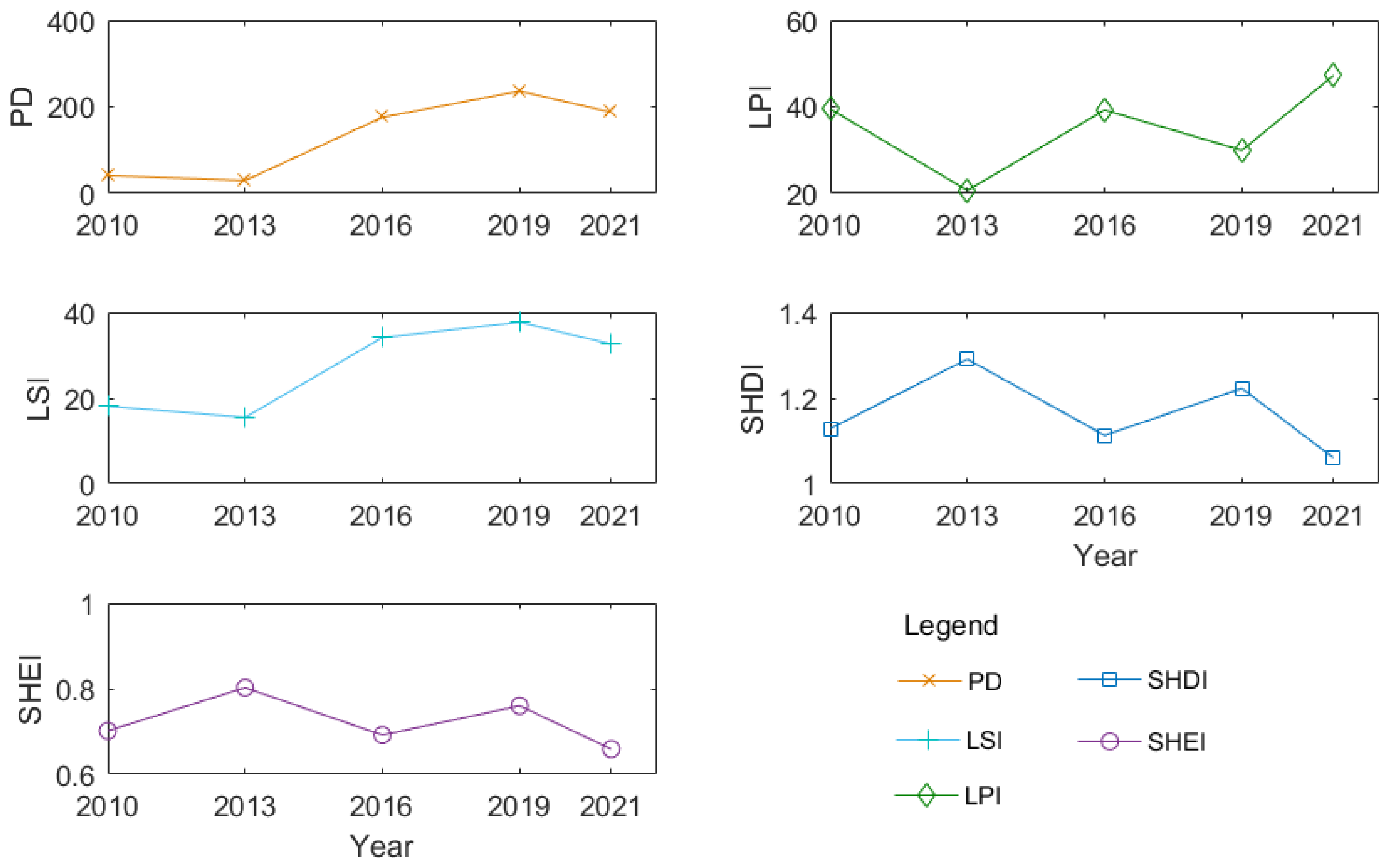
| Year | Item | PLAND | NP | PD | LPI | LSI |
|---|---|---|---|---|---|---|
| 2010 | Built-up | 11.66 | 169.00 | 8.39 | 3.47 | 18.08 |
| Forest land | 61.24 | 124.00 | 6.16 | 39.52 | 14.23 | |
| Farm land | 17.09 | 387.00 | 19.21 | 1.47 | 28.61 | |
| Bare land | 1.71 | 95.00 | 4.72 | 0.36 | 10.33 | |
| Water area | 8.29 | 55.00 | 2.73 | 3.81 | 9.43 | |
| 2013 | Built-up | 33.91 | 110.00 | 5.26 | 20.68 | 17.25 |
| Forest land | 42.25 | 131.00 | 6.26 | 19.55 | 14.43 | |
| Farm land | 2.88 | 242.00 | 11.57 | 0.18 | 16.71 | |
| Bare land | 14.37 | 101.00 | 4.83 | 8.51 | 10.18 | |
| Water area | 6.59 | 34.00 | 1.62 | 2.43 | 7.82 | |
| 2016 | Built-up | 42.87 | 645.00 | 32.24 | 39.26 | 40.87 |
| Forest land | 43.88 | 1166.00 | 58.28 | 10.32 | 39.04 | |
| Farm land | 1.03 | 682.00 | 34.09 | 0.16 | 26.71 | |
| Bare land | 5.67 | 855.00 | 42.74 | 1.82 | 30.03 | |
| Water area | 6.55 | 169.00 | 8.45 | 2.68 | 11.00 | |
| 2019 | Built-up | 41.20 | 927.00 | 46.34 | 29.94 | 45.22 |
| Forest land | 39.35 | 1546.00 | 77.28 | 8.92 | 37.80 | |
| Farm land | 1.41 | 799.00 | 39.94 | 0.10 | 28.74 | |
| Bare land | 10.81 | 1201.00 | 60.03 | 4.35 | 37.10 | |
| Water area | 7.24 | 257.00 | 12.85 | 3.61 | 14.69 | |
| 2021 | Built-up | 51.54 | 579.00 | 28.56 | 47.24 | 37.74 |
| Forest land | 37.37 | 1228.00 | 60.58 | 8.57 | 36.36 | |
| Farm land | 1.28 | 956.00 | 47.16 | 0.09 | 33.19 | |
| Bare land | 4.34 | 640.00 | 31.57 | 1.28 | 28.81 | |
| Water area | 5.47 | 396.00 | 19.54 | 2.51 | 1.13 |
| Stage | Period | Time Range | Characteristics of Land Change | Ecological Maintenance |
|---|---|---|---|---|
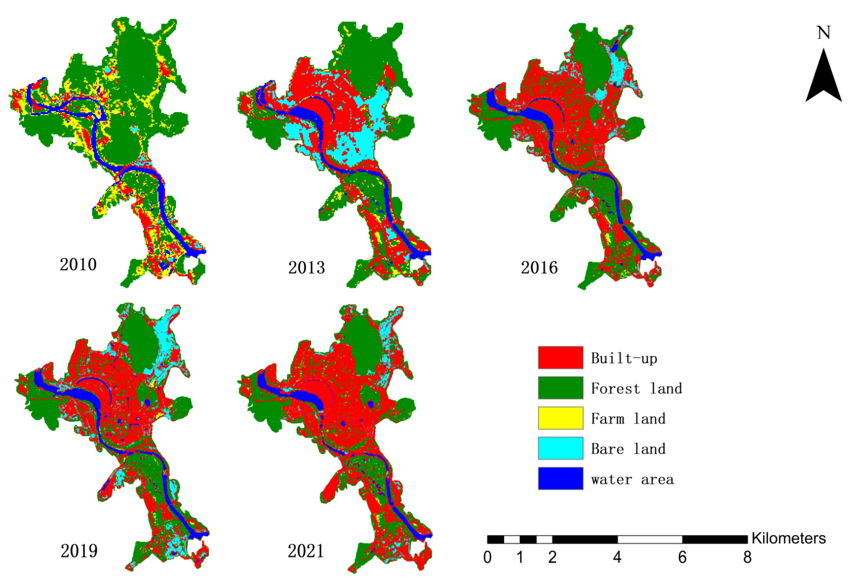
| The first stage | Development and expansion period | 2010–2013 | Forest land and farm land decrease, while built-up and bare land increase (with great changes); the expansion strength is large and the change speed is fast | RSEI excellent grade decreases significantly, and the decline degree is mainly medium; FVC is mainly decreased; the heterogeneity and uniformity of landscape increase, but the degree of fragmentation and shape index do not change much. The two forest lands in the northeast and west of Renshan area have always been the most undeveloped ecological protection areas. The ecological quality fluctuates greatly in the middle of Renshan area |
| Construction and conservation period | 2013–2016 | The forest land is basically unchanged, the bare land decreases and the built-up land increases; rapid construction of built-upland ; the intensity and rate of change are large | RSEI remains unchanged and the downward trend is controlled; FVC remains unchanged and rises; the uniformity and diversity of landscape decreases while the degree of fragmentation and shape index increase | |
| The second stage | Development and expansion period | 2016–2019 | Mainly the forest land and bare land increase (change small compared with 2010–2013); the intensity and rate of change decrease | RSEI is mainly unchanged with the phenomenon of ecological quality recovery; FVC is mainly constant; the diversity and uniformity of landscape are increased, and the degree of fragmentation and complexity of landscape shape are controlled |
| Construction and conservation period | 2019–2021 | Mainly an increase in built-up land and the decrease in bare land (small change); the intensity and rate of change decrease | RSEI remains unchanged and tends to be stable as a whole; FVC is mainly constant and tends to be stable; landscape diversity and uniformity decreases, fragmentation degree and shape index decrease |
Publisher’s Note: MDPI stays neutral with regard to jurisdictional claims in published maps and institutional affiliations. |
© 2022 by the authors. Licensee MDPI, Basel, Switzerland. This article is an open access article distributed under the terms and conditions of the Creative Commons Attribution (CC BY) license (https://creativecommons.org/licenses/by/4.0/).
Share and Cite
Han, R.; Sha, J.; Li, X.; Lai, S.; Lin, Z.; Lin, Q.; Wang, J. Remote Sensing Analysis of Ecological Maintenance in Subtropical Coastal Mountain Area, China. Remote Sens. 2022, 14, 2734. https://doi.org/10.3390/rs14122734
Han R, Sha J, Li X, Lai S, Lin Z, Lin Q, Wang J. Remote Sensing Analysis of Ecological Maintenance in Subtropical Coastal Mountain Area, China. Remote Sensing. 2022; 14(12):2734. https://doi.org/10.3390/rs14122734
Chicago/Turabian StyleHan, Run, Jinming Sha, Xiaomei Li, Shuhui Lai, Zejing Lin, Qixin Lin, and Jinliang Wang. 2022. "Remote Sensing Analysis of Ecological Maintenance in Subtropical Coastal Mountain Area, China" Remote Sensing 14, no. 12: 2734. https://doi.org/10.3390/rs14122734
APA StyleHan, R., Sha, J., Li, X., Lai, S., Lin, Z., Lin, Q., & Wang, J. (2022). Remote Sensing Analysis of Ecological Maintenance in Subtropical Coastal Mountain Area, China. Remote Sensing, 14(12), 2734. https://doi.org/10.3390/rs14122734