Article

Probabilistic Evaluation of Slope Reliability Considering Groundwater Level Uncertainty Based on Dynamic Agent Model Using Uniform Design

1
School of Civil Engineering, Lanzhou University of Technology, Lanzhou 730050, China
2
College of Geology Engineering and Geomatics, Chang’an University, Xi’an 710054, China
*
Author to whom correspondence should be addressed.
Remote Sens. 2022, 14(12), 2779; https://doi.org/10.3390/rs14122779
Submission received: 9 May 2022 / Revised: 6 June 2022 / Accepted: 6 June 2022 / Published: 9 June 2022

Abstract

:
Due to the adverse influence of landslide disasters on human lives, property, and infrastructures, slope reliability analysis has attracted worldwide attention. However, many problems such as the neglect of the uncertainty in the water table level and the balance between the performance and efficiency in conventional models are still unresolved. This study investigates the influence of the uncertainty in the water table level on the benefit of considering such uncertainty in slope reliability analysis. For this purpose, a new method, i.e., a dynamic whale optimization algorithm (WOA)–Gaussian process regression (GPR) agent model using uniform design with the consideration of uncertainty in the groundwater level, is proposed for slope probabilistic analysis in this paper. Then the developed technique is integrated with Monte Carlo Simulation (MCS) to obtain the slope failure probability. The benefit of the proposed method is illustrated through two practical landslides. The results demonstrate that the developed technique has better performance, as compared to MCS, the v-support vector machine (v-SVR), and the generalized regression neural network (GRNN). This may be attributed to the dynamic updating of the training samples provided by the uniform design, the optimal hyper-parameters optimized by WOA, or the GPR model that has strong generalization ability with limited samples. Furthermore, a small failure probability is obtained without considering the groundwater level uncertainty, which offers an optimistic estimate of landslide stability. Therefore, it is necessary to consider the probabilistic features of the groundwater level, especially for complicated landslides in high mountainous areas where the location of the water table level is not accurately available due to their inaccessibility to people and instruments.

1. Introduction

At present, landslides have not only imposed huge direct economic losses on industrial and agricultural production and the safety of human lives and properties but have also resulted in incalculable indirect losses due to the suspension of amphibious transportation. Therefore, it is urgent to conduct effective early-warning research on landslides, where the reliability of slope stability analysis has been an important prerequisite. However, various categories of inevitable uncertainties (e.g., the boundary conditions uncertainty, geological model uncertainty, soil parameter uncertainty, and external trigger uncertainty) may pose an important influence on accurate slope reliability, where the soil properties uncertainty accounts for a major contribution to the probability of failure [1,2,3,4,5,6,7].
To offer a rational and convincing assessment of slope stability, scholars have made numerous efforts to integrate probability and statistic theories with the traditional slope reliability assessment approaches with consideration of the subsurface uncertainties [8,9,10,11,12,13]. For example, Low et al., (1997) developed a new method with the application of spreadsheets to calculate the Hasofer–Lind second moment [14]. Cho (2013) adopted a first-order reliability method (FORM) to evaluate the slope stability considering multiple failure modes [10]. Jiang et al., (2015) studied the slope stability with a low probability of failure in spatially variable soils based on MCS [15]. However, the above-mentioned methods are only effective in the case that the issues have explicit limit state function. Although MCS had proven its ability to address cases with implicit limit state function or a low probability of failure [16,17,18,19,20,21], it might encounter some limitations such as substantial computational efforts and a complicated procedure, particularly for issues with a low probability of failure.
Agent model-based response surface methods (RSMs) [22,23,24,25,26,27] can make compensations for the shortcomings of MCS. Cho (2009), Li et al., (2013), and Kang et al., (2015, 2016, 2017) proposed a procedure by integrating numerical analyses such as FEM and LEM into the reliability analysis for complicated slopes [22,28,29,30,31]. They employed an artificial neural network (ANN), SVR, and extreme learning machine (ELM)-based RSMs to substitute the real performance function. The failure probability was obtained from the agent model in connection with MCS. Unfortunately, these studies paid extensive attention to the uncertainty of soil properties but lacked investigations on the probabilistic characteristics of the water table level, which may greatly contribute to the probability of slope failure. In reality, the usual practice considers the water table level as a constant and proceeds with probabilistic analysis. This practice, which neglects such uncertainty, may produce an obvious deviation concerning the slope reliability, especially for complex landslides with an unknown water table level in high mountainous areas where people and instruments find it difficult to access. More importantly, extensive data are required to construct a sufficiently accurate RSM. For instance, for ANN-based RSM, 20 training samples were used to accurately establish the RSM for slope with three random variables, whereas 150 samples were needed for issues with four random variables [28]. Although the training samples adopted to establish an effective SVM and ELM-based RSMs [22,26] were reduced to fifteen times the random variables considered, the sample size generated was still large.
Alternatively, the GPR agent model offers a better choice. The merits of this technique over the other machine-learning techniques had been extensively discussed by Seeger (2008); Su et al., (2009); Kang et al., (2017) [30,32,33]. Furthermore, this study will illustrate that limited samples are able to construct a sufficiently accurate GPR-based RSM, which is much smaller than that needed by ANN, SVM, or ELM [
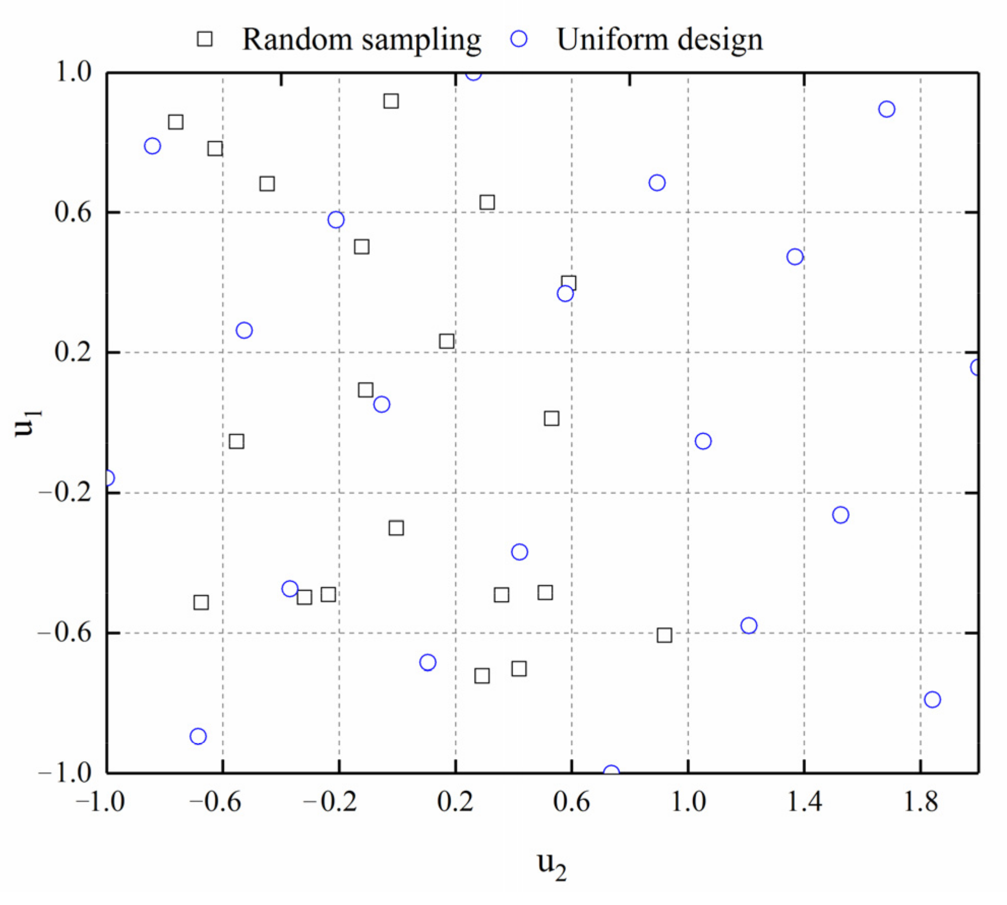
34]. Nonetheless, the samples are frequently generated by a random approach [35], which may not ensure that the selected samples scatter in the domain uniformly. More importantly, most of the RSMs in the available literature are constructed only based on training samples extracted once, which may, in turn, lower the accuracy of the constructed method, and even increase the computational effort when the sample size is small or the extrapolated testing samples exceed the training sample space.
Further, the hyper-parameters of the covariance function for GPR play an important role in model performance, which depends on the extent of parameter optimization. The conjugate gradient method is often used to search the hyper-parameters. However, it may encounter several limitations, such as over-dependence on the initial value, difficulty in determining the number of iterations, and local optimization [36]. The issues may be extremely severe since the best parameters for GPR are customarily unavailable.
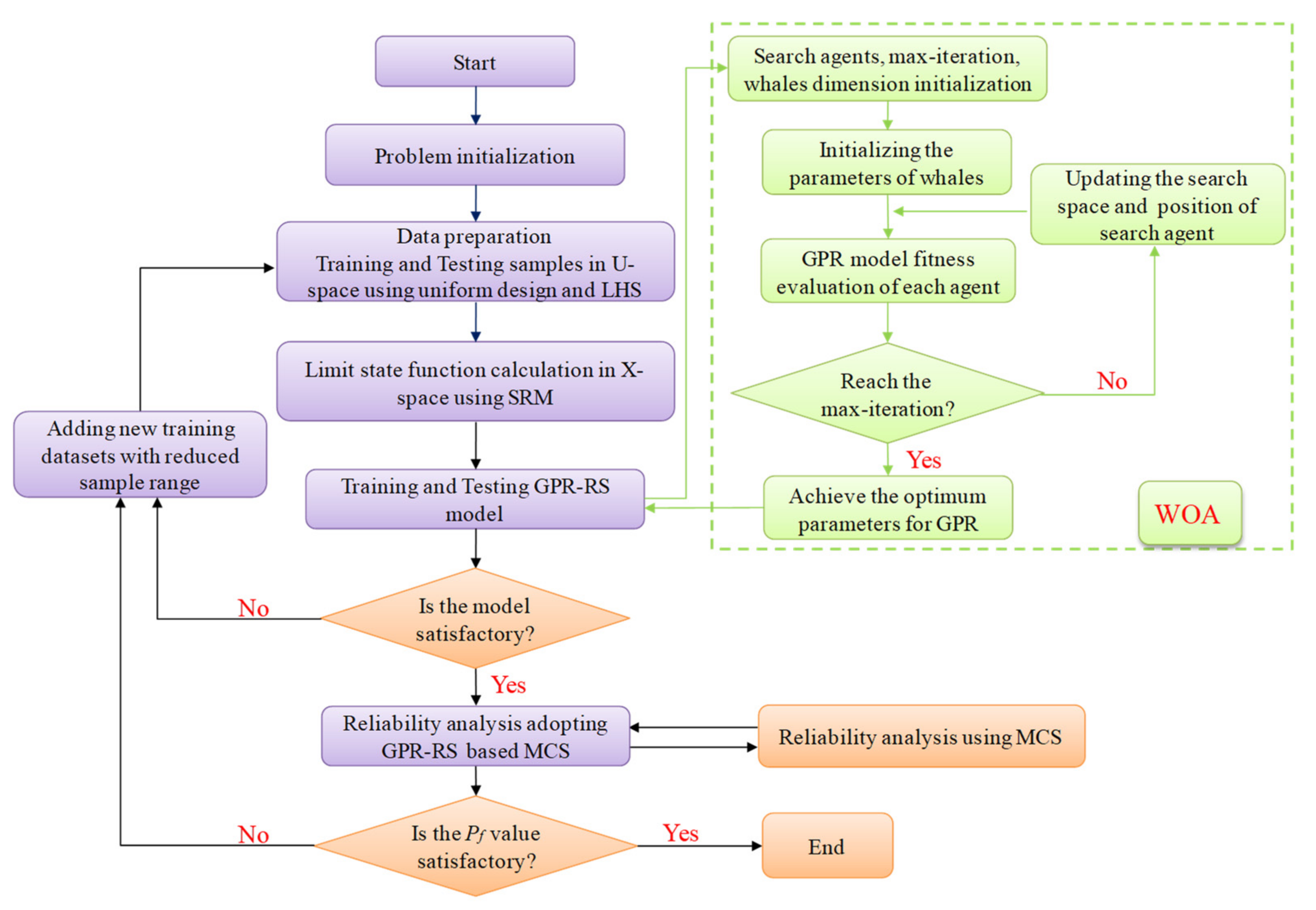
Hence, to address the aforementioned issues, this study develops a practical procedure, i.e., a dynamic WOA-GPR RSM based on a uniform design that considers the uncertainty of the water table level [
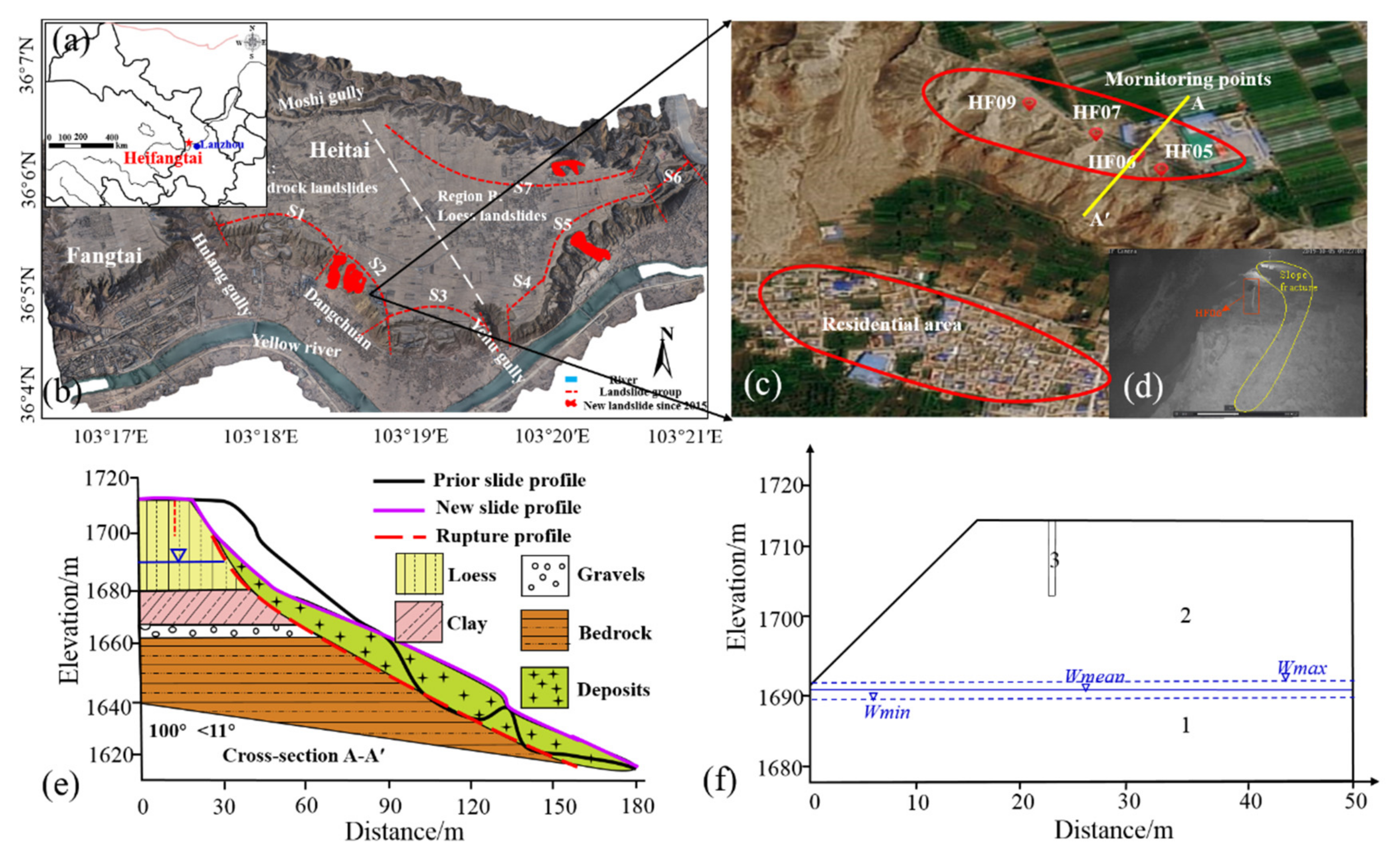
37]. One of the main purposes of this research is to investigate the significance and benefits of considering such uncertainty in slope reliability analysis, particularly for high mountainous areas where people and instruments find it hard to reach, and to improve the model performance and efficiency through iteration. This study is also devoted to improving the accuracy and efficiency of the current RSMs. Two practical slopes are selected as the case studies, which have been reported by several researchers [38,39,40]. Accordingly, sufficient field monitoring data are available to compare and verify the slope stability analysis. Conventional methods such as MCS, v-SVR, and GRNN are adopted for comparison [41,42]. The results demonstrate that with the consideration of the uncertainty of the water table level, the developed model obtains a reasonable probability of failure. At the same time, the application of an iterative algorithm has reduced the number of representative samples selected by the uniform design and consequently improved the accuracy and efficiency of GPR RSM. WOA, which is able to jump out of the local optimum, is adopted to achieve the optimal hyper-parameters for GPR. In conclusion, this dynamic WOA-GPR-based RSM with consideration of the water table level uncertainty, which has not been investigated previously by other researchers, offers an effective way for complicated slope reliability analysis.

2. Methodology

2.1. Slope Reliability Analysis Using MCS

Probabilistic and statistic approaches that consider geological uncertainties are frequently adopted to evaluate slope stability. Assume that vector x = x 1 , x 2 , , x m (m denotes the number of random variables) are the uncertain parameters (random variables) for the slope, and the slope failure probability ( P f ) is obtained from the following Equation:
P f = P g x 0 = g x 0 f x d x
where f x is the joint probability density function, and g x denotes the slope limit state function.
The limit state function g(x) is expressed as:
Z = g x = F s x 1
where F s x denotes the factor of safety determined by the strength reduction method (SRM).
Accordingly, the slope reliability analysis can be implemented with the P f obtained from Equation (1). However, for complicated slopes with high nonlinearity, Equation (1) is impossible to be addressed by direct integration. Hence, MCS that uses massive statistic samples is adopted for substitution. The expression of P f determined by MCS is as follows:
P f 1 N i = 1 N I g x i 0
where N is the sample size and x i is the i-th sample. Besides, I · represents the indicative function of g x . When the slope slides, g x 0 , I · = 1 , and otherwise, I · = 0 .
Accordingly, the unbiased estimation of slope failure probability can be obtained from MCS with sufficient samples. Unfortunately, deterministic slope stability analysis based on SRM is required for each sample, which is time-consuming. Besides, MCS is also not applicable to estimate slopes with low failure probability that need even more samples, as compared to those with high failure probability.
Therefore, this paper presents a sufficiently accurate WOA-GPR RSM to calculate the F s x of a small number of representative samples. The g x i is subsequently obtained from the following Equation:
g x i = F W O A G P R x i 1
where F W O A G P R x i represents the factor of safety of the i-sample obtained from WOA-GPR.
By substituting Equation (4) into Equation (3), the landslide failure probability and its variation coefficient determined by MCS can be obtained from Equations (5) and (6).
P f 1 N i = 1 N I g x i 0 = 1 N i = 1 N I F W O A G P R x i 0
C O V P f = 1 P f N P f

2.2. Gaussian Process Regression (GPR)

GPR determines the conditional distribution of the target output by inferring the relation between the input vector and the target output vector for the training dataset based on Bayesian theory [32,43,44]. It has a collection of various merits such as good generalization ability and easy implementation and is suitable for solving nonlinear regression problems with limited samples and high dimensions [44,45,46].
Given a training dataset D = x i , y i | i = 1 , 2 , , n = X , y , where xi is the input of the i-th sample and y i represents the output of the i-th sample, the model is defined as follows:
y = f x + ε
where ε denotes the white noise that obeys a Gaussian distribution, namely, ε ~ N ( 0 , σ n 2 ) .
It is known that a Gaussian process is entirely determined by its mean and covariance function. To simplify the calculation, the mean is set as zero. Hence, the expression of the Gaussian process is obtained as follows:
f ~ G P ( 0 , k ( x , x ) )
where k ( x , x ) is the covariance function of Gaussian progress.
According to the Bayesian principle, within a given training dataset D, the prior distribution of y can be determined by Equations (7) and (8):
y ~ N ( 0 , K + σ n 2 I )
where K = K X , X = k x i , x j m × m and denotes a symmetric positive definite covariance matrix, and I is the unit matrix.
Accordingly, the joint Gaussian distribution between the training samples and a given test sample can be defined as shown in Equation (10).
y y * ~ N 0 , K X , X + σ n 2 I K X , x * K x * , X K x * , x *
where X represents the training input vector, x * is one of the input feature vectors of the test samples, and y * is the output of the test sample. Besides,   K X 1 , X 2 denotes the n 1 × n 2 –order covariance function matrix obtained from the datasets in X 1 and those in X 2 , in which n i is the sample (column) number of X i .
Based on the obtained joint Gaussian distribution in Equation (10), the posterior probability distribution of the output value y * is calculated from the mean function y ^ * and covariance function c o v ( y * ) :
y * | X , y , x * ~ N ( y ^ * , c o v ( y * ) )
where y ^ * and c o v ( y * ) for GPR can be expressed as:
y ^ * = K x * , X K X , X + σ n 2 I 1 y
c o v ( y * ) = K x * , x * K x * , X K X , X + σ n 2 I 1 K X , x *
For the posterior distribution, the mean y ^ * represents the optimum value of y * and c o v ( y * ) offers the estimation confidence. For instance, the 95% confidence interval of the predictions is calculated as [ y ^ * 1.96 c o v ( y * ) , y ^ * + 1.96 c o v ( y * ) ]. Accordingly, the GPR technique can not only provide accurate predictions, but also give the uncertainty estimation of the predictions.
Besides, since the mean value of the Gaussian process is 0, the accuracy of GPR depends completely on the type of covariance function that satisfies Mercer’s theorem. In other words, the covariance function provides the estimation confidence. In this paper, based on the performance of several commonly used kernel functions, the Rational Quadratic covariance function (RQ) with better performance is adopted to construct a GPR model.
k R Q x i , x j = σ f 2 1 + x i x j 2 P 2 α α + σ n 2 δ i j
where δ i j is the Kronecker delta function, P is the product matrix of the length-scale function ι 2 and I , σ f represents the variance of the kernel function, and α denotes the relative weighting of large-scale and small-scale variations. The optimal hyper-parameters Θ = P , σ f , α are generally achieved from the conjugate gradient method adaptively. However, there have several limitations to this approach, such as over-dependence on the initial value, the difficulty in determining the number of iterations, and local optimization [35]. Hence, WOA is adopted to achieve the optimal parameters of GPR in this paper.

2.3. Whale Optimization Algorithm (WOA)

WOA is a new meta-heuristic swarm intelligence optimization algorithm presented by Mirjalili and Lewis (2016) [37]. It has several prominent merits such as a simple principle and fewer parameters and is liable to jump out of the local optimum. This algorithm simulates the “spiral bubble-net” feeding strategy of humpback whales to hunt their prey by following its location and encircling the prey (Figure 1).
The detailed searching procedures are as follows.
In the first step, due to the unknown optimal position, the algorithm suggests that the current best candidate location is the target prey or close to the optimal solution [37,47]. Once the best search individual has been identified, other search individuals will attempt to move to the best position. Equations (15) and (16) demonstrate this behavior:
D = C · X * t X t
X ( t + 1 ) = X * t A · D
where t is the current iteration, X ( t ) is the location vector of the prey, and X * ( t ) denotes the location vector for the best solution and should be updated when a better solution is obtained in each iteration.
Besides, A   and C are coefficient vectors that are defined in Equations (17) and (18).
A = 2 a · r r
C = 2 · r
where a   is decreased linearly from 2 to 0 during the iterative stage and r denotes a random vector within 0 , 1 .
In the second stage, i.e., the development stage, the humpback whales adopt either a shrink encircling mechanism or a spiral model with a 50% probability when the whale’s position is updated. This behavior is illustrated by the following Equation:
X ( t + 1 ) = X * t A · D   i f   p 0.5 D · e b l · cos 2 π l + X * t   i f   p 0.5  
where D = X * t X t and denotes the distance between the i-th whale and the prey, b is the type of the logarithmic spiral, and l is a random value that falls into [−1, 1].
At the exploration stage, humpback whales search the prey randomly based on each other’s location. To assure the best solution can be obtained from WOA, random numbers ( A ) that are either smaller than −1 or greater than 1 are adopted to force the search agent to stay away from the reference prey [47]. When A is greater than 1, the algorithm is still in the exploration stage. On the contrary, unlike the development phase, the location of the search agent is updated based on the randomly selected search agent rather than the best search agent found so far, allowing the WOA algorithm to perform a global search. The position-updating Equations are as follows:
D = C · X r a n d t X t
X t + 1 = X r a n d t A · D
where X r a n d t   denotes the random vector selected from the current species group.
At the same time, the objective function-root mean square error ( R M S E ) (Equation (22)) is adopted to obtain the optimal parameters. The global optimal solution of the GPR model (the position of the prey) is then obtained when the maximum iteration or the predefined iterative criterion is reached. Figure 2 illustrates a brief flowchart of WOA.
R M S E = 1 n i = 1 n y ^ i y i 2
where n   denotes the number of observations, y ^ i   is the predicted i-th value, and y i   is the actual observed values.

2.4. Model Performance Evaluation

The indices, namely the Nash–Sutcliffe Efficiency ( N S E ) [48], variance account factor ( V A F ) [49], coefficient of determination ( R 2 ), adjusted R 2 ( R A d j 2 ) [50], relative percentage difference ( R P D ) [51], performance index ( P I ) [52], and Willmott’s index ( W I ) [53], are applied to assess the performances of the discussed techniques in this paper. Detailed expressions of the abovementioned measures are shown as follows:
N S E = 1 i = 1 n y ^ i y i 2 i = 1 n y i y m e a n 2
V A F = 1 v a r y ^ i y i v a r y i
R 2 = n i = 1 n y ^ i y i i = 1 n y ^ i i = 1 n y i 2 n i = 1 n y ^ i 2 i = 1 n y ^ i 2 n i = 1 n y i 2 i = 1 n y i 2
R A d j 2 = 1 n 1 n p 1 1 R 2
P I = R A d j 2 + 0.01 V A F R M S E
W I = 1 i = 1 n y ^ i y i 2 i = 1 n y ^ i y i + y i y m e a n 2
R P D = S D R M S E
where y m e a n is the observed mean values, v a r denotes the variance, p is the number of regression coefficients, and S D is the standard deviation
The above measures are explained as follows: The closer the N S E , V A F , R 2 , R A d j 2 , and W I values are to 1, the better the model performs. For P I , which represents the comprehensive performance of a method, a value of 2 shows that the model performs excellently. The lower the R M S E , the better the model performs. Besides, the values of R P D divided by Viscarra Rossel et al., (2006) [51] are presented in Table 1.

2.5. Dynamic WOA-GPR Response Surface Framework Using Uniform Design

Generally, the more variables and the higher the nonlinearity of the performance function, the more samples are needed to establish an accurate RSM model. In other words, extensive samples are required to construct a sufficient RSM model for slopes with more random variables or problems with higher nonlinearity. On the other hand, to ensure the high precision of RSM, the training samples selected should cover the distribution interval of random variables uniformly. Therefore, to reduce the calculation cost, researchers used experimental designs such as the central composite design to produce limited sampling points for the RSM [54]. However, the performance of the constructed model may not be satisfactory once the samples are too small, the spatial distribution of the samples is unreasonable, or the extrapolated testing samples exceed the training sample space. In conclusion, the main limitation of the traditional approach is the large number of training samples needed to establish an adequately precise RSM technique.
To obtain the best performance through the least number of points, the uniform design [55,56,57] is adopted to generate the training samples that are scattered uniformly within the range. For example, the 20 points generated by the uniform design within the range [–1, 1] are scattered uniformly in 20 grids with each grid containing one sample (Figure 2). On the contrary, an identical number of points obtained from random sampling is scattered randomly, which may increase the number of samples to build a comparatively accurate RSM. Thus, in this paper, we propose an iterative procedure to construct a dynamic RSM using thee uniform design for lower computational cost. At the first iteration, the sampling range is evenly divided in the U-space (i.e., independent standard normal distribution space) according to the sample size and factor levels. Then the random variables obtained in the U-space are shifted to those in the X-space as illustrated in Low et al., (2011) and Lue et al., (2012) [21,58]. We use Latin Hypercube Sampling (LHS) to generate the testing points. All the points are adopted to establish and test the WOA-GPR model. In the next iteration, we reduce the width of the sampling range and the number of sampling points. The iteration will not be stopped until the convergence requirement is satisfied.
In conclusion, given the aforementioned limitations in the published studies, an iterative procedure based on uniform design is presented, where the number of training samples is slightly increased and thus achieved from the astringency of the problems considered. Figure 3 illustrates the procedure of slope reliability analysis considering groundwater level uncertainty based on the WOA-GPR dynamic RSM using the uniform design.

3. Results

In the published literature, the majority of the slope stability evaluations are focused on uncertainties in soil properties, ignoring the probabilistic characteristics of the water table level that may make a significant contribution to the probability of slope failure. Shadabfar et al., (2020) [59] considered the uncertainty in groundwater level, but only simplified the water table and did not combine it with the model. Hence, for reliable slope stability analysis, the location of the water table level is defined as a stochastic variable in this study. The slope safety factors for all samples are obtained from SRM using the finite difference method. Then the WOA-GPR dynamic RSM is constructed based on the sampling points produced by uniform design. The failure probability is subsequently obtained from the developed technique when combined with MCS. Two practical slopes are adopted for model verification. The number of sampling points is also gradually increased to illustrate the reliability of the constructed RSM output. Besides, the v-SVR and GRNN-based RSM are also applied for comparison.

3.1. Case 1: Lodalen Slope

Lodalen landslide took place on 6 October 1954, in the region of the Lodalen marshalling yard near the Oslo railway station [39,60]. Since then, several excavations and reconstructions had been operated on the landslide. Before it collapsed, the landslide was 17 m high with a slope angle of 26° (2H: 1V). Figure 4 depicts the geometric profile of the landslide before the time of failure. More detailed descriptions of this slope can be found in previous reports [13,39,40]. The statistical information of this case is shown in Table 2. All random variables of the slope obey a normal distribution. The water table, determined by a blue solid-line as shown in Figure 4, is obtained by the Equation y = 0.003 x 2 0.078 x + 22.765 (where x is the horizontal axis and y is the vertical axis).
For a slope that has many random variables and a high fluctuation of variables, extensive training samples are required to establish an adequately precise RSM. As the number of samples required is previously unknown, the training procedure should start with comparatively limited samples. Then the number of training samples is gradually increased to update the training sample set until the convergence requirement is satisfied. Accordingly, for the Lodalen slope, the WOA-GPR approach is established with the initial 21 samples within the range [–3, 3] determined by the uniform design, which are scattered evenly in the domain. The factors of safety for all training samples are calculated from SRM. Then a temporary WOA-GPR model is constructed according to the training samples (model input) and corresponding factors of safety (model output). In the next iteration, the number of training samples is reduced by half and evenly distributed within the interval [−2, 2]. Figure 5 and Figure 6 present the prediction error in the factor of safety and RMSE obtained from WOA-GPR with different samples and cycles, respectively. Concerning the training points, the results of two cycles for different samples are comparable to that of three cycles except for 32-2 training. The results of testing points show a similar pattern. However, considering the overall performance it is obvious that the accuracy of the WOA-GPR technique constructed by two iterations is close to that of the model established by three iterations. The nearly equal results illustrate the uselessness of increasing the time of cycles. In other words, the increase in the number of iterations causes a slight difference in the performance of the developed approach. The attempt to improve the model accuracy significantly through three cycles might be in vain. Therefore, two iterations can afford to build an RSM with acceptable accuracy for the Lodalen slope.
Table 3 shows the parameters of different algorithms for Lodalen slope. Then the performances of WOA-GPR, v-SVR, and GRNN models constructed by two iterations with different initial samples are calculated and listed in Table 4. The results of the statistical measures ( N S E , R 2 , R A d j 2 , V A F , P I , R P D , W I ) illustrate that the accuracies of the discussed models are greatly improved with the increase in training samples. However, considering the results for the same samples, the WOA-GPR has the best performance, followed by the v-SVR and GRNN.
Figure 7 presents the errors of the factor of safety obtained from GPR, v-SVR, and GRNN methods. Figure 8 displays the Taylor Diagram of training and testing results in terms of the standard deviation and correlation (the sqrt of R 2 ), where the black circle denotes the references, while the others denote the predictions. The closer the predictions are to the reference data, the higher the accuracy of the discussed model will be. Accordingly, as for the training procedure, the proposed method and v-SVR show comparable accuracy, while the GRNN has a bad performance. However, the best performance is recorded in the developed technique in the testing stage. Moreover, compared to the v-SVR and GRNN, the proposed approach performs better with fewer samples. For instance, 38 training samples are required to build an accurate GPR model, while 52 training samples are needed for both v-SVR and GRNN models. Hence, the presented model is superior to the other two models in accuracy and efficiency.
Besides, for WOA-GPR, the increase in sampling points may contribute little to the improvement in model precision. The comparable performance of the developed model with 42 and 45 points illustrates the inefficiency of increasing training samples. More importantly, according to the outcomes calculated from MCS (Table 5), the presented method with 42 samples is sufficient to substitute the real limit state function of the Lodalen slope.
Accordingly, based on the dynamic WOA-GPR model with 42 sampling points, a total of 1 × 10⁵ samples are generated by MCS based on the probabilistic distribution of random variables. The histogram and the cumulative probability density for the factor of safety obtained from the MCS are shown in Figure 9a,b, respectively. It is obvious that the factor of safety by the proposed method obeys a normal distribution, which is in accordance with the distribution of random variables.
Table 6 shows the results of failure probability achieved in the published literature for an identical problem. Compared to the results obtained from the v-SVR and GRNN, the failure probability of 26.67% obtained from this paper is closer to that determined by Shadabfar et al. in 2020 [59]. However, if the water table remains the same, the instability probability is only 21.36%, which is smaller than that obtained from this paper. We would achieve an optimal outcome in this case. The deviations between the two scenarios illustrate the importance and benefit of considering the groundwater level uncertainty. As the failure probability for the Lodalen slope could increase under the effect of groundwater level uncertainty, it is necessary to establish such uncertainty for accurate slope stability analysis. In conclusion, with the consideration of the uncertainty in the water table, reliable failure probability with high precision is achieved from the presented model in this study.

3.2. Case 2: Dangchuan Landslide in Heifangtai

Given the results for the Lodalen slope in Case 1, the proposed approach has good applicability in the reliability analysis for practical slopes with consideration of the uncertainty in the groundwater level. Therefore, the model is used to assess the stability of the landslide in Heifangtai, China. The slope failure occurred in the vicinity of Dangchuan No.6 and No.7 landslides, Gansu Province, China, where landslide disasters took place frequently. Figure 10 is the simplified geometric profile of the Dangchuan landslide. More detailed geological descriptions of the landslide can be obtained from [42]. The soil properties are reported in Table 7. Besides, the uncertainty in groundwater level is also considered as a random variable that obeys an assumed normal distribution, where the mean and variance are 13 m and 0.3 m, respectively.
Considering the results of Lodalen slope in Case 1, the more random variables and the larger variation of random variables, the bigger the number of training samples required to establish an accurate RSM. On the contrary, fewer sampling points are needed for slopes with a small number of random variables. Accordingly, the initial samples should be reduced since there are only three random variables in this example. Take the experiment with 23 samples as an example. In the first iteration, 15 sampling points are provided by the uniform design, and 8 points within the reduced sample interval are added to the training samples in the subsequent iteration. Figure 11 and Figure 12 present the prediction error in the factor of safety and R M S E obtained from WOA-GPR with different samples and cycles, respectively. It is obvious that the developed model performs well in the same initial samples of two and three cycles for the training and testing stages, indicating that two iterations can afford the accuracy requirement of RSM for the Dangchuan landslide.
Table 8 shows the parameters of different algorithms for Case 2. Then the performances of the three models with gradually increased samples are calculated and reported in Table 9. The errors in the factor of safety and the Taylor Diagram of training and testing results obtained from GPR, v-SVR, and GRNN methods are shown in Figure 13 and Figure 14. It is evident that the predictions determined by the three models show good agreement with those obtained from SRM in model training. Nevertheless, when it comes to the model testing stage, the performance is in favor of the developed technique ( N S E , R 2 , R A d j 2 , V A F , P I , R P D , W I ). Moreover, considering the results with identical samples, the developed model has the best performance in model testing, followed by v-SVR and GRNN.
Then an MCS with 1 × 10⁵ samples is implemented by adopting the developed RSM based on the probabilistic distribution of random variables. Table 10 shows the failure probabilities estimated from GPR, v-SVR, and GRNN methods with different sample sizes. According to the results obtained from MCS in Table 10, 28 sampling points are sufficient to build an accurate GPR model, which is much smaller as compared to those required to construct the v-SVR and GRNN models. Besides, the histogram and the cumulative probability density for the factor of safety based on the dynamic WOA-GPR model with 28 sampling points are in good agreement with the actual normal distribution as illustrated in Figure 15a,b. In conclusion, the developed dynamic WOA-GPR RSM based on the uniform design in this paper is superior to v-SVR and GRNN-based RSMs in accuracy and computational effort, which further verifies the feasibility of the proposed method to evaluate slope reliability.
Overall, the method presented in this paper can aptly approximate the real performance function. Hence, MCS based on the proposed RSM is conducted to calculate the slope failure probability. Table 11 presents the results achieved from the published literature for the same issue. As shown, the obtained failure probability for the Dangchuan landslide is closer to the value determined by MCS, as compared with both the value of 9.22% reported by v-SVR and that of 9.99% obtained from GRNN. Besides, when the groundwater level was defined as a constant, Ling et al. obtained a 23.57% reduction in the failure probability of the landslide in 2021 [42]. This indicates the significant influence of groundwater uncertainty on the failure probability. The slope reliability would be overestimated without considering the uncertainty in the water table level, especially when its position is difficult to be determined. Hence, it is essential to explore the probabilistic characteristics of the water table level in addition to the uncertainties in soil properties.

4. Discussion

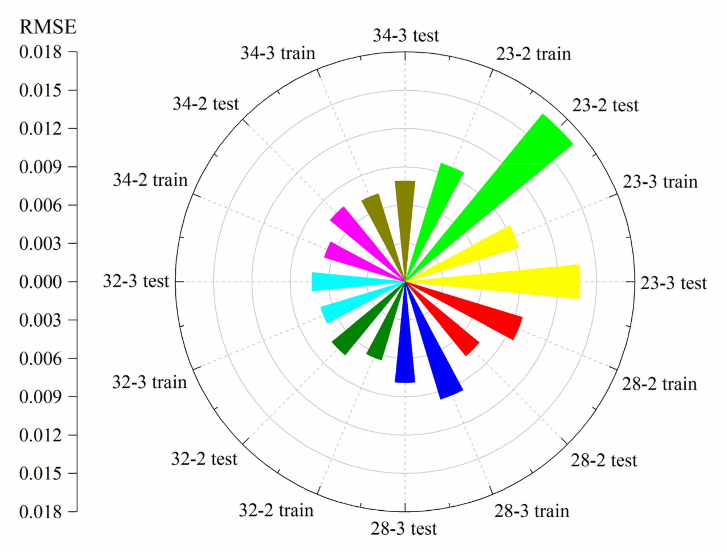
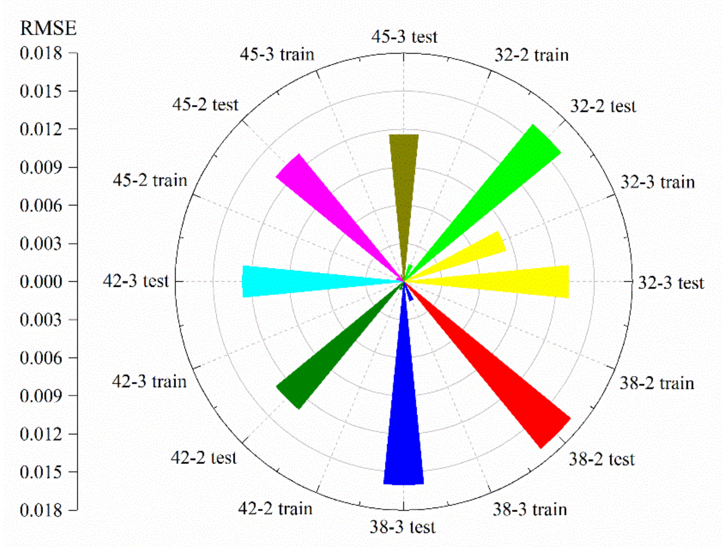
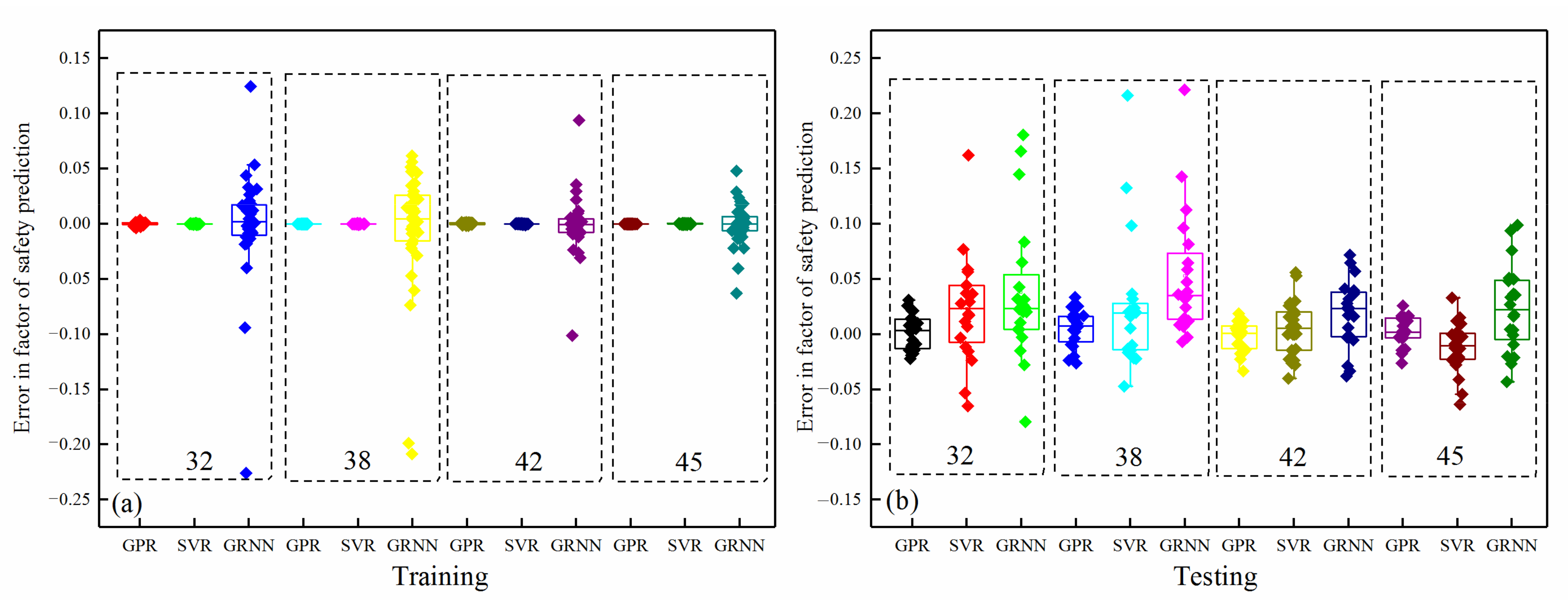
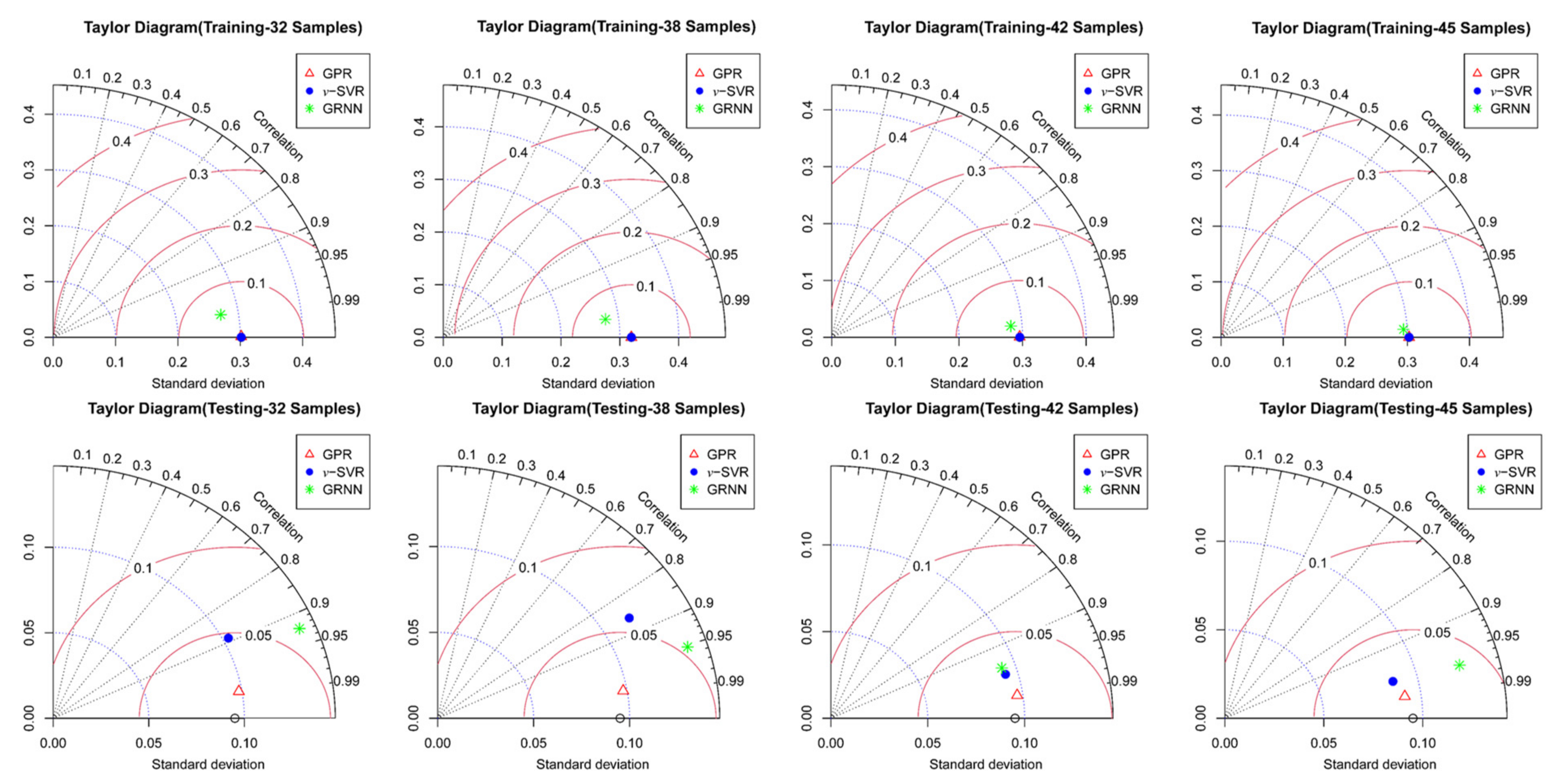
Achieving a precise RSM for a complicated slope has been a hot topic in recent decades. Machine-learning-based RSMs are demonstrating promising applicability in addressing such issues with the development of artificial intelligence. Accordingly, we present a dynamic WOA-GPR RSM to analyze landslide reliability in this study. An iterative procedure based on uniform design is adopted to reduce the number of sampling points. Then we implement an extensive comparison (over seven indices) to assess the performances of GRNN, v-SVR, and GPR-based RSMs through two practical landslides. As shown in Table 4 and 
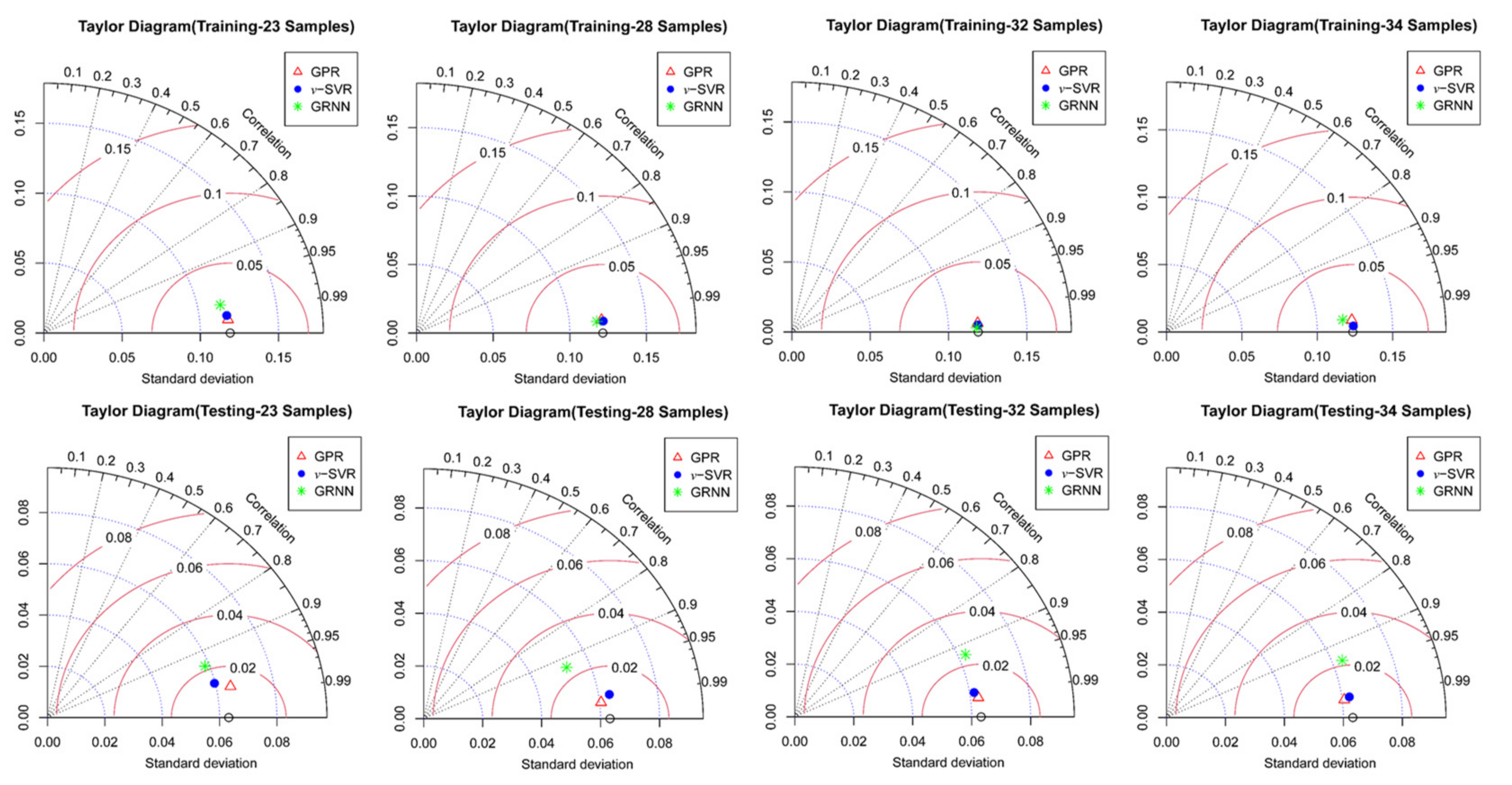
Table 9, it is clear that the presented technique performs better compared to the other two techniques in terms of the indices illustrated in Equation (23) to Equation (29). At the same time, the Taylor diagram, which offers the degree of approximation between the actual and predicted data in terms of standard deviation and their correlation, is also plotted for training and testing datasets as illustrated in Figure 8 and Figure 13. According to the results and analysis in Section 3, the WOA-GPR-based RSM yields the best predictions as compared with the GRNN and v-SVR-based models. Besides, slight deviations in failure probability obtained from our method and MCS are reported in both cases. In summary, our approach is superior to the other models discussed with respect to accuracy.
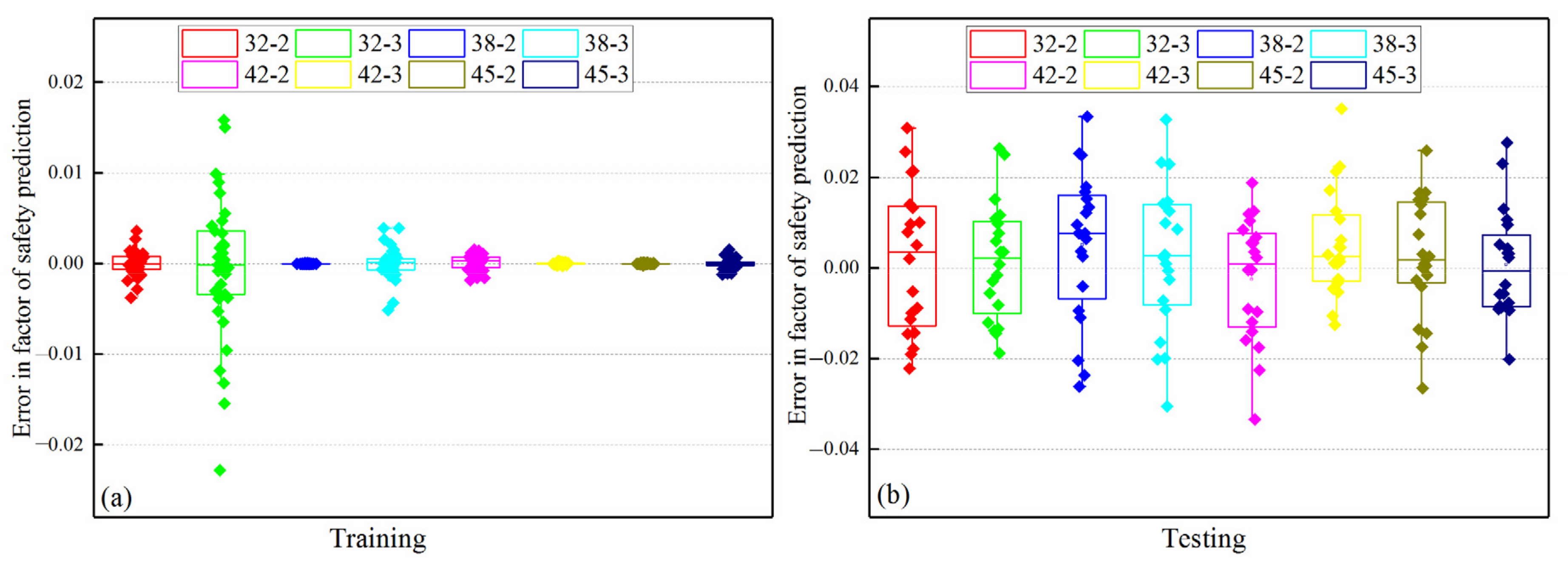
To achieve rapid results, we implement an iterative algorithm based on a uniform design. Notably, the results of the two cases show that the number of training samples is reduced to a relatively small level, i.e., 42 samples for Case 1 and 28 samples for Case 2. This means that for issues with three and four random variables, our study reduces 17 and 18 samples as compared to the studies in [22,26,29,30,42], which need 45 and 60 samples to construct an accurate RSM, respectively. Accordingly, the iterative procedure can effectively improve the efficiency of our method. Besides, considering the approximate accuracy, our model requires much fewer sampling points to establish an accurate RSM for both cases. This demonstrates that the WOA-GPR model is efficient for landslide reliability analysis. From what has been discussed above, we can reasonably conclude that our approach performs better in comparison with the GRNN and v-SVR models in terms of computation effort.
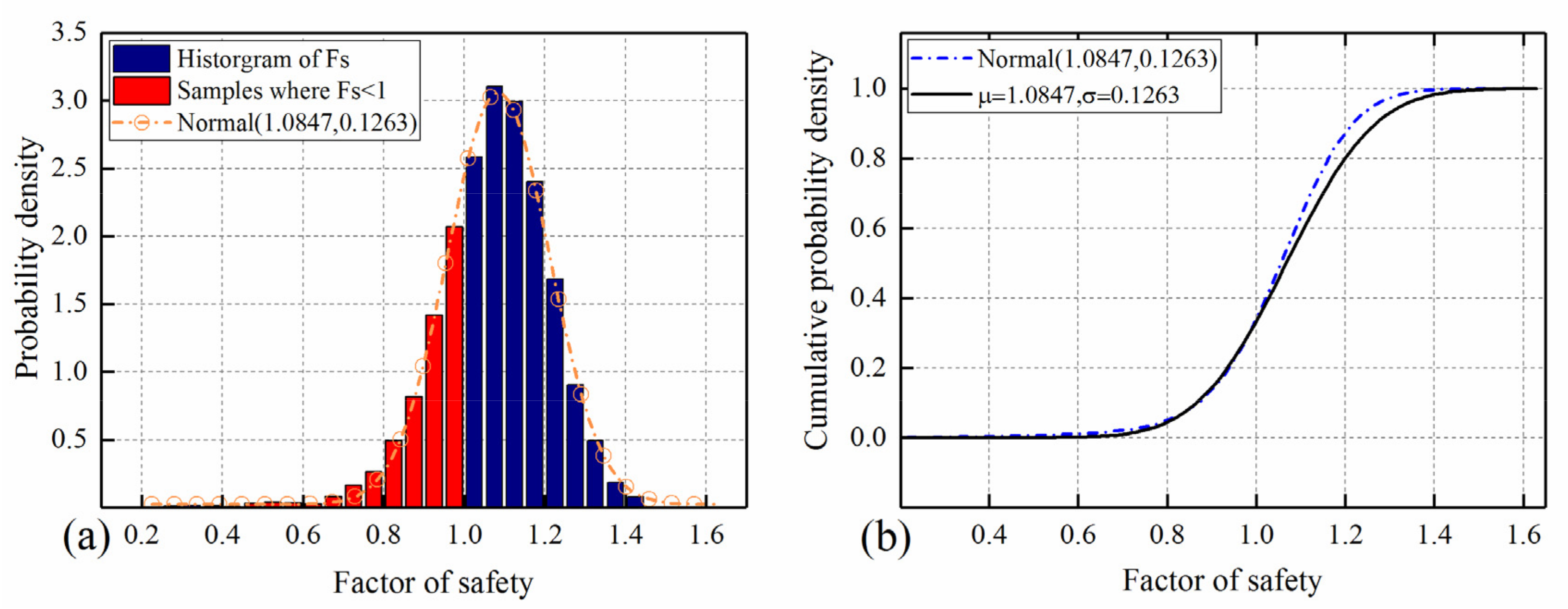
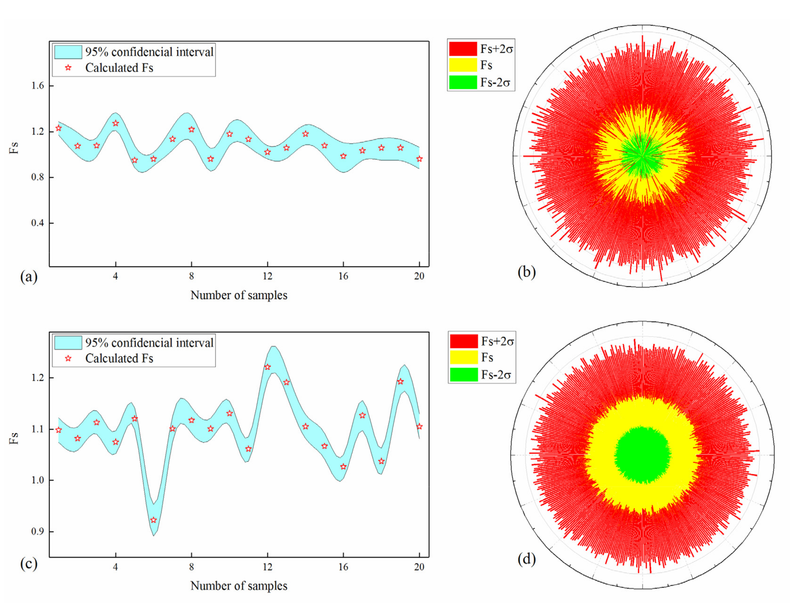
Further, as compared with the other methods, our study can not only provide the factor of safety, but also offers sufficient confidence levels. Figure 16a,c shows the factor of safety ( F s ) calculated from SRM and 95% confidence levels of F s obtained from dynamic WOA-GPR RSM for the two landslides. Figure 16b,d presents the Fs and the corresponding 95% confidential level determined by the proposed model when combined with MCS with 5000 samples for both cases. As shown, all the values of Fs fall into the 95% confidential interval obtained from the dynamic WOA-GPR RSM using the uniform design.
Additionally, the uncertainty in the water table level appears to have a larger contribution to the increase in failure probability in our case studies. In other words, a small failure probability is achieved in the absence of water table level uncertainty, which is in agreement with the previous literature reported in [59]. We may obtain an optimistic assessment of landslide stability and fail to predict future landslide occurrence. Hence, for slopes in which it is hard to determine their water table level, it is reliable to consider such uncertainty, especially in high mountainous areas where people and equipment find it hard to reach.
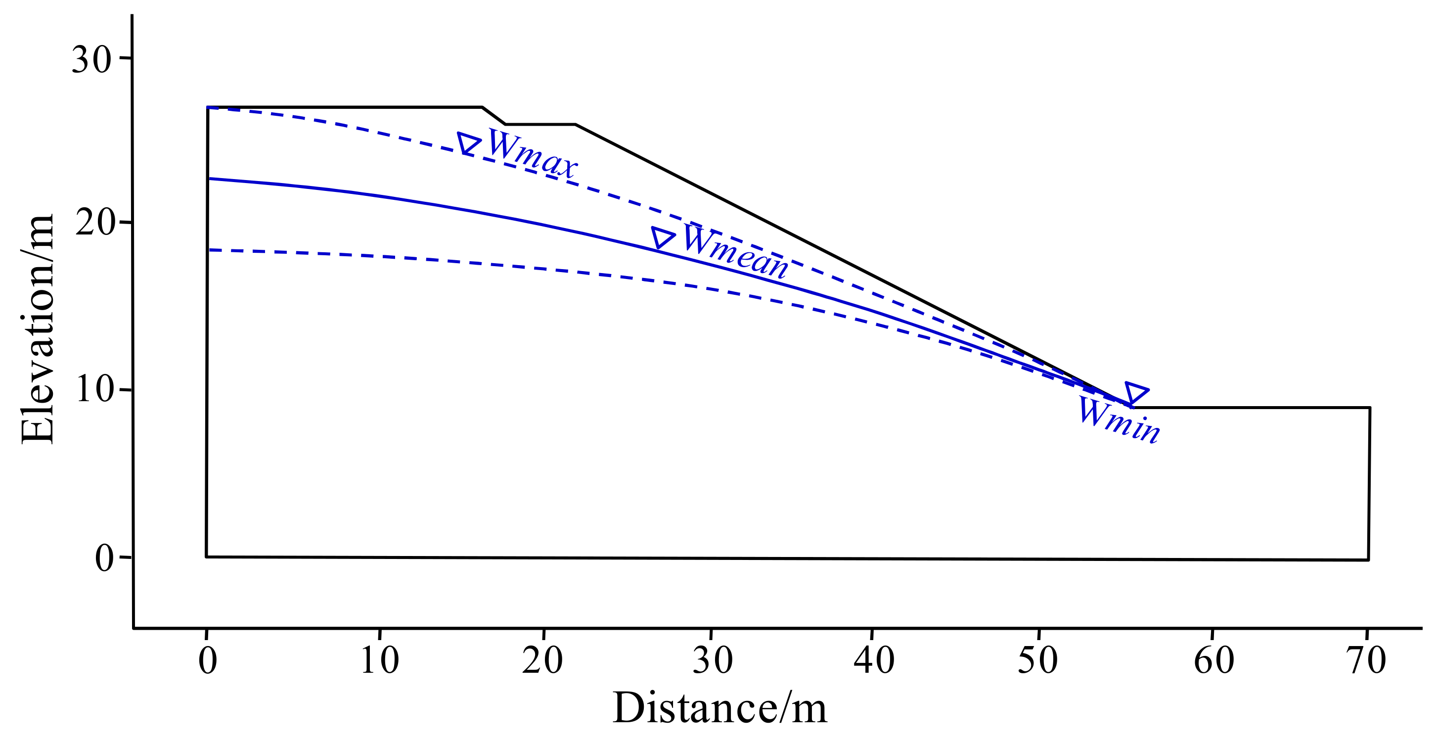
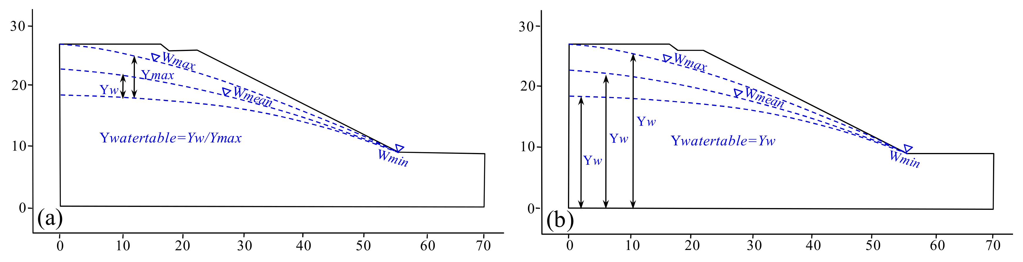
Besides, the failure probability of the Lodalen slope achieved in this paper is slightly higher than the value of 26.06% determined by Shadabfar et al., (2020) [59]. This might be ascribed to the factor of safety obtained from different methods of Simplified Bishop and SRM, or to the dissimilar application of the water table level as shown in Figure 17.
We also investigate the impact of the type of groundwater level distribution on failure probability. Table 12 shows the values for the water table level with assumed distribution functions for both slopes. Results obtained from our model with a uniform distribution are different from those determined by the other three distribution functions. Besides, the approximate failure probability is determined by the proposed method with the normal, lognormal, and triangular distribution functions, where the result with a normal distribution offers a more optimistic assessment of the landslide stability.
In this study, since the reliability evaluation based on MCS is independent of the factor of slope safety using SRM, other available methods such as LEM and the Simplified Bishop can also be adopted to implement the developed technique. Besides, the required samples are found to be 42 for Case 1 with four random variables, and the samples are 28 for Case 2 with three random variables. For problems with more than five random variables, experimental results show that it is quite possible to increase the times of cycles to implement probabilistic analysis, which will be further studied in the future.

5. Conclusions

Accurate and efficient slope stability analysis can improve the accuracy of landslide early warnings, thus reducing the casualties and damage to properties from such disasters. For decades, machine-learning-based RSMs have been developed for probabilistic analysis of landslides, including ANN, SVM, KELM, and so on. However, it is still a challenging task to determine an efficient method from the machine-learning-based RSMs, which would help researchers accurately analyze slope reliability and thus help benefit human lives and property safety. Besides, most studies rarely consider the uncertainty in the underground water table, which has become a crucial element absent in slope stability assessment.
One of the contributions of this study is the development of a new method that adds the uncertainty in groundwater level to existing approaches of slope reliability analysis and facilitates the researcher to uncover the hidden patterns and regularities in the deformation of landslides. We adopted a uniform design to construct a dynamic WOA-GPR-based RSM model. Two practical landslides, i.e., the Lodalen slope and Dangchuan landslide, were chosen to verify the applicability of the developed technique. For the case studies illustrated in the study, we found that the water table level uncertainty made higher contributions to offering reliable results. Besides, with the aid of a uniform design and a new iterative dynamic RSM, we are able to save large amounts of time in terms of reducing the samples generated for the construction of the WOA-GPR-based RSM. We are also able to reduce the number of iterative times the RSM is established. Considering the overall performance, our method has proven to be the best model, since it produced higher results with lower computation time, and significantly outperformed the GRNN and v-SVR-based RSMs. The technique developed in this research is a new hybrid approach for landslide stability analysis, which combines the merits of uniform design and WOA and GPR models. The results in this paper show the potential usability of the developed method in evaluating the stability of slopes that are difficult in terms of determining their underground water levels, especially in high mountainous areas where people and equipment find it hard to reach. The novel technique can also be applied to similar geological scenarios for landslide risk reduction.
In conclusion, machine-learning-based RSMs show promising applicability in landslide reliability analysis. The assessment of such hazards is vital for landslide mitigation and prevention. The results achieved can help researchers to better understand the influences of different types of uncertainties encountered in landslides, and thus help disaster emergency management departments to implement effective measures to reduce the potential risks to an acceptable degree. In the future, methods to address problems with more than five random variables still need to be validated through different cases by investigating proper measures such as the increase in iterations. In addition, in order to realize early landslide warnings, real-time monitoring data of a higher resolution will be integrated into the WOA-GPR framework in the future.

Author Contributions

Conceptualization, Q.L. and Q.Z.; methodology, Q.L. and W.Q.; model test and validation, Q.L.; formal analysis, Q.L. and J.Z.; writing—original draft preparation, Q.L. and Q.Z.; writing—review and editing, Q.L., Q.Z., W.Q. and J. Z. All authors have read and agreed to the published version of the manuscript.

Funding

This research was funded by the National Natural Science Foundation of China (NSFC) (grant nos: 42127802, 41731066, 42174006, 42090055), the Science Fund for Distinguished Young Scholars of Shaanxi Province (grant no: 2022JC-18), the Science and Technology Plan of Gansu Province in China (grant no: 20JR10RA180), and the Leading Talents Program of Central Universities (grant no. 300102261302).

Data Availability Statement

Restrictions apply to the availability of the data. Data are available from authors with the permission of Q.Z. and Q.L.

Acknowledgments

I would like to express my gratitude to all those who helped me during the writing of this thesis. A special acknowledgement should be shown to Mahdi Shadabfar, from whose data and suggestions I benefited greatly.

Conflicts of Interest

The authors declare no conflict of interest.

References

  1. Mann, C. Uncertainty in Geology. Computers in Geology—25 Years of Progress; Oxford University Press: New York, NY, USA, 1993; pp. 241–254. [Google Scholar]
  2. Bardossy, G.; Fodor, J. Traditional and new ways to handle uncertainty in geology. Nat. Resour. Res. 2001, 10, 179–187. [Google Scholar] [CrossRef]
  3. Ching, J.Y.; Wang, J.S. Application of the transitional Markov chain Monte Carlo algorithm to probabilistic site characterization. Eng. Geol. 2016, 203, 151–167. [Google Scholar] [CrossRef]
  4. Dou, Z.; Liu, Y.M.; Zhang, X.Y.; Wang, Y.S.; Chen, Z.; Wang, J.G.; Zhou, Z.F.; Xiong, H. Influence of layer transition zone on rainfall-induced instability of Multilayered slope. Lithosphere 2021, 2021, 2277284. [Google Scholar] [CrossRef]
  5. Yeh, C.H.; Dong, J.J.; Khoshnevisan, S.; Juang, C.H.; Huang, W.C.; Lu, Y. The role of the geological uncertainty in a geotechnical design–A retrospective view of Freeway No. 3 Landslide in Northern Taiwan. Eng. Geol. 2021, 291, 106233. [Google Scholar] [CrossRef]
  6. Bossi, G.; Borgatti, L.; Gottardi, G.; Marcato, G. Quantification of the uncertainty in the modelling of unstable slopes displaying marked soil heterogeneity. Landslides 2019, 16, 2409–2420. [Google Scholar] [CrossRef]
  7. Tao, Z.G.; Geng, Q.; Zhu, C.; He, M.; Cai, H.; Pang, S.H.; Meng, X.Z. The mechanical mechanism of large-scale toppling failure for counter-inclined rock slopes. J. Geophys. Eng. 2019, 16, 541–558. [Google Scholar] [CrossRef] [Green Version]
  8. Cornell, C.A. First-order uncertainty analysis of soils deformation and stability. In Proceedings of the 1st International Conference on Application of Statistics and Probability to Soil and Structural Engineering, Hong Kong, China; 1971; pp. 130–144. [Google Scholar]
  9. Christian, J.T.; Ladd, C.L.; Baecher, G.B. Reliability Applied to Slope Stability Analysis. J. Geotech. Engrg. 1994, 120, 2180–2207. [Google Scholar] [CrossRef]
  10. Cho, S.E. First-order reliability analysis of slope considering multiple failure modes. Eng. Geol. 2013, 154, 98–105. [Google Scholar] [CrossRef]
  11. Low, B.K.; Tang, W.H. Efficient spreadsheet algorithm for first-order reliability method. J. Eng. Mech. 2007, 133, 1378–1387. [Google Scholar] [CrossRef]
  12. Low, B.K. FORM, SORM, and spatial modeling in geotechnical engineering. Struct. Saf. 2014, 49, 56–64. [Google Scholar] [CrossRef]
  13. Suchomel, R.; Mašín, D. Comparison of different probabilistic methods for predicting stability of a slope in spatially variable c–φ soil. Comput. Geotech. 2012, 7, 132–140. [Google Scholar] [CrossRef]
  14. Low, B.K.; Tang, W.H. Efficient reliability evaluation using spreadsheet. J. Eng. Mech. 1997, 123, 749–752. [Google Scholar] [CrossRef]
  15. Jiang, S.H.; Li, D.; Cao, Z.; Zhou, C.; Phoon, K. Efficient system reliability analysis of slope stability in spatially variable soils using Monte Carlo simulation. J. Geotech. Geoenviron. 2015, 141, 04014096. [Google Scholar] [CrossRef]
  16. El-Ramly, H.; Morgenstern, N.R.; Cruden, D. Probabilistic assessment of stability of a cut slope in residual soil. Géotechnique 2005, 55, 77–84. [Google Scholar] [CrossRef]
  17. Su, G.S.; Zhao, W.; Peng, L.; Yan, L. Gaussian process-based dynamic response surface method for estimating slope failure probability. Rock Soil Mech. 2014, 32, 3592–3601. [Google Scholar] [CrossRef]
  18. Tamimi, S.; Amadei, B.; Frangopol, D. Monte Carlo simulation of rock slope reliability. Comput. Struct. 1989, 33, 1495–1505. [Google Scholar] [CrossRef]
  19. Song, S.Y.; Zhao, M.Y.; Zhu, C.; Wang, F.Y.; Cao, C.; Li, H.J.; Ma, M.Y. Identification of the potential critical slip surface for fractured rock slope using the FLOYD algorithm. Remote Sens. 2022, 14, 1284. [Google Scholar] [CrossRef]
  20. Wang, Y.; Cao, Z.J.; Au, S.K. Practical reliability analysis of slope stability by advanced Monte Carlo Simulations in a spreadsheet. Can. Geotech. J. 2011, 48, 162–172. [Google Scholar] [CrossRef]
  21. Lue, Q.; Chan, C.L.; Low, B.K. Probabilistic evaluation of ground-support interaction for deep rock excavation using artificial neural network and uniform design. Tunn. Undergr. Space Technol. 2012, 32, 1–18. [Google Scholar] [CrossRef]
  22. Kang, F.; Li, J.S. Artificial bee colony algorithm optimized support vector regression for system reliability analysis of slopes. J. Comput. Civ. Eng. 2016, 30, 04015040. [Google Scholar] [CrossRef]
  23. Zhang, X.; Zhu, C.; He, M.C.; Dong, M.L.; Zhang, G.C.; Zhang, F.M. Failure mechanism and long short-term memory neural network model for landslide risk prediction. Remote Sens. 2022, 14, 166. [Google Scholar] [CrossRef]
  24. Piliounis, G.; Lagaros, N.D. Reliability analysis of geostructures based on metaheuristic optimization. Appl. Soft Comput. 2014, 22, 544–565. [Google Scholar] [CrossRef]
  25. Ru, Z.L.; Zhao, H.B.; Zhu, C.X. Probabilistic evaluation of drilling rate index based on a least square support vector machine and Monte Carlo simulation. Bull. Eng. Geol. Environ. 2019, 78, 3111–3118. [Google Scholar] [CrossRef]
  26. Song, L.F.; Yu, X.; Xu, B.; Pang, R.; Zhang, Z.Y. 3D slope reliability analysis based on the intelligent response surface methodology. Bull. Eng. Geol. Environ. 2021, 80, 735–749. [Google Scholar] [CrossRef]
  27. Tan, X.H.; Bi, W.H.; Hou, X.L.; Wei, W. Reliability analysis using radial basis function networks and support vector machines. Comput. Geotech. 2011, 38, 178–186. [Google Scholar] [CrossRef]
  28. Cho, S.E. Probabilistic stability analyses of slopes using the ANN based response surface. Comput. Geotech. 2009, 36, 787–797. [Google Scholar] [CrossRef]
  29. Kang, F.; Han, S.X.; Salgado, R.; Li, J.S. System probabilistic stability analysis of soil slopes using Gaussian process regression with Latin hypercube sampling. Comput. Geotech. 2015, 63, 13–25. [Google Scholar] [CrossRef]
  30. Kang, F.; Li, J.S.; Wang, Y.; Li, J.J. Extreme learning machine-based surrogate model for analyzing system reliability of soil slopes. Eur. J. Environ. Civ. Eng. 2017, 21, 1341–1362. [Google Scholar] [CrossRef]
  31. Li, S.J.; Zhao, H.B.; Ru, Z.L. Slope reliability analysis by updated support vector machine and Monte Carlo simulation. Nat. Hazards 2013, 65, 707–722. [Google Scholar] [CrossRef]
  32. Seeger, M. Gaussian processes for machine learning. Int. J. Neural. Syst. 2008, 14, 69–106. [Google Scholar] [CrossRef] [Green Version]
  33. Su, G.S.; Song, Y.C.; Yan, L.B. Application of Gaussian process machine learning to slope stability evaluation. Rock Soil Mech. 2009, 30, 103–107. [Google Scholar] [CrossRef]
  34. Zhu, C.; Karakus, M.; He, M.C.; Meng, Q.X.; Shang, J.L.; Wang, Y.; Yin, Q. Volumetric deformation and damage evolution of Tibet interbedded skarn under multistage constant-amplitude-cyclic loading. Int. J. Rock Mech. Min. 2022, 152, 105066. [Google Scholar] [CrossRef]
  35. Goh, A.T.; Kulhawy, F.H. Reliability assessment of serviceability performance of braced retaining walls using a neural network approach. Int. J. Numer. Anal. Met. 2005, 29, 627–642. [Google Scholar] [CrossRef]
  36. Xu, C.; Liu, B.G.; Liu, K.Y.; Guo, J.Q. Intelligent analysis model of landslide displacement time series based on coupling PSO-GPR. Rock Soil Mech. 2011, 32, 1669–1675. [Google Scholar] [CrossRef]
  37. Mirjalili, S.; Lewis, A. The whale optimization algorithm. Adv. Eng. Softw. 2016, 95, 51–67. [Google Scholar] [CrossRef]
  38. El-Ramly, H.; Morgenstern, N.R.; Cruden, D.M. Lodalen slide: A probabilistic assessment. Can. Geotech. J. 2006, 43, 956–968. [Google Scholar] [CrossRef]
  39. Gitirana, J.G.; Santos, M.A.; Fredlund, M.D. Three-dimensional analysis of the Lodalen landslide. In Proceedings of the GeoCongress 2008, New Orleans, LA, USA, 9–12 March 2008; pp. 186–190. [Google Scholar] [CrossRef] [Green Version]
  40. Ling, Q.; Zhang, Q.; Wei, Y.; Kong, L.J.; Zhu, L. Slope reliability evaluation based on multi-objective grey wolf optimization-multi-kernel-based extreme learning machine agent model. Bull. Eng. Geol. Environ. 2021, 80, 2011–2024. [Google Scholar] [CrossRef]
  41. Specht, D. A general regression neural network. IEEE T. Neural Networ. 1991, 2, 568–576. [Google Scholar] [CrossRef] [Green Version]
  42. Zhang, P.; Zhang, D.F.; Yang, Y.; Zhang, W.G.; Wang, Y.W.; Pan, Y.J.; Liu, X.Z. A case study on integrated modeling of spatial information of a complex geological body. Lithosphere 2022, 2022, 2918401. [Google Scholar] [CrossRef]
  43. Sofiane, B.; Amine, B. Gaussian process for non-stationary times series prediction. Comput. Stat. Data An. 2004, 47, 705–712. [Google Scholar] [CrossRef]
  44. Rasmussen, C.; Williams, C. Gaussian Processes for Machine Learning; MIT Press: Cambridge, MA, USA, 2006. [Google Scholar]
  45. Rasmussen, C. Gaussian processes in machine learning. In Proceedings of the Summer School on Machine Learning, Tubingen, Germany, 4–16 August 2003; pp. 63–71. [Google Scholar]
  46. Snelson, E. Flexible and Efficient Gaussian Process Models for Machine Learning. Ph.D. Thesis, Gatsby Computational Neuroscience Unit, University College London, London, UK, 2007. [Google Scholar]
  47. Hassan, G.; Hassanien, A.E. Retinal fundus vasculature multilevel segmentation using whale optimization algorithm. Signal Image Video P. 2018, 12, 263–270. [Google Scholar] [CrossRef]
  48. Nash, J.; Sutcliffe, J. River flow forecasting through conceptual models part I—A discussion of principles—ScienceDirect. J. Hydrol. 1970, 10, 282–290. [Google Scholar] [CrossRef]
  49. Alvarez, G.A.; Babuska, R. Fuzzy model for the prediction of unconfined compressive strength of rock samples. Int. J. Rock Mech. Min. Sci. 1999, 36, 339–349. [Google Scholar] [CrossRef]
  50. Babu, G.L.; Srivastava, A. Reliability analysis of allowable pressure on shallow foundation using response surface method. Comput. Geotech. 2007, 34, 187–194. [Google Scholar] [CrossRef]
  51. Viscarra Rossel, R.A.; Mcglynn, R.N.; Mcbratney, A.B. Determining the composition of mineral-organic mixes using UV-vis-NIR diffuse reflectance spectroscopy. Geoderma. 2006, 137, 70–82. [Google Scholar] [CrossRef]
  52. Ray, R.; Kumar, D.; Samui, P.; Roy, L.B.; Goh, A.T.; Zhang, W.G. Application of soft computing techniques for shallow foundation reliability in geotechnical engineering. Geosci. Front. 2020, 12, 375–383. [Google Scholar] [CrossRef]
  53. Willmott, C.J. Some comments on the evaluation of model performance. Bull. Am. Meteorol. Soc. 1981, 2, 219–232. [Google Scholar] [CrossRef] [Green Version]
  54. Wong, F. Slope reliability and response-surface method. J. Geotech. Eng. Div. 1985, 111, 32–53. [Google Scholar] [CrossRef]
  55. Fang, K.T. The uniform design: Application of number-theoretic methods in experimental design. Acta Math. Appl. Sin. 1980, 3, 363–372. [Google Scholar]
  56. Fang, K.T. Uniform Design and Uniform Design Tables; Science Press: Beijing, China, 1991. [Google Scholar]
  57. Wang, Y.; Fang, K.T. A note on uniform distribution and experimental design. A Mon. J. Sci. 1981, 26, 485–489. [Google Scholar] [CrossRef]
  58. Low, B.K.; Zhang, J.; Tang, W.H. Efficient system reliability analysis illustrated for a retaining wall and a soil slope. Comput. Geotech. 2011, 38, 196–204. [Google Scholar] [CrossRef]
  59. Shadabfar, M.; Huang, H.W.; Kordestani, H.; Muho, E.V. Reliability analysis of slope stability considering uncertainty in water table level. ASCE-ASME J. Risk Uncertain. Eng. Syst. Part A 2020, 6, 04020025. [Google Scholar] [CrossRef]
  60. Hassan, A.M.; Wolff, T. Search algorithm for minimum reliability index of earth slopes. J. Geo. Geoenviron. 1999, 125, 301–308. [Google Scholar] [CrossRef]
  61. Peng, D.L.; Xu, Q.; Liu, F.Z.; He, Y.S.; Zhang, S.; Qi, X.; Zhao, K.Y.; Zhang, X.L. Distribution and failure modes of the landslides in Heitai terrace, China. Eng. Geol. 2018, 236, 97–110. [Google Scholar] [CrossRef]
Figure 1. Bubble-net feeding behavior of humpback whales.
Remotesensing 14 02779 g001
Figure 2. Distribution of samples produced by uniform design and random sampling.
Remotesensing 14 02779 g002
Figure 3. Slope reliability analysis considering groundwater level uncertainty based on the WOA-GPR dynamic RSM using uniform design.
Remotesensing 14 02779 g003
Figure 4. Geometric profile of the Lodalen slope.
Remotesensing 14 02779 g004
Figure 5. The error in factor of safety prediction obtained from WOA-GPR with different samples and cycles (here 32-2 denotes two cycles with 32 samples): (a) Training; (b) testing.
Remotesensing 14 02779 g005
Figure 6. RMSE obtained from WOA-GPR with different samples and cycles for Case 1.
Remotesensing 14 02779 g006
Figure 7. Case 1: Errors of factor of safety obtained from GPR, v-SVR, and GRNN methods by employing (a) training points; (b) testing points.
Remotesensing 14 02779 g007
Figure 8. Taylor diagram of training and testing obtained from WOA-GPR, v-SVR, and GRNN.
Remotesensing 14 02779 g008
Figure 9. Results of MCS with 5 × 10⁴ samples for Case 1: (a) Histogram and normal fit for the obtained factor of safety with a normal distribution of random variables; (b) probability density distribution for the obtained factor of safety.
Remotesensing 14 02779 g009
Figure 10. (a) Location of the study region (red star); (b) aerial view of the Heifangtai with landslide sections (image photo on 18 January 2015) [61]; (c) distribution of monitoring points and residential area; (d) monitored slope fracture in HF06; (e) lithological profile of cross-section A-A′; (f) geometric profile of the cross-section A-A′ (1 denotes saturated loess, 2 denotes unsaturated loess, 3 denotes the crack).
Remotesensing 14 02779 g010
Figure 11. The error in factors of safety prediction obtained from WOA-GPR with different samples and cycles (here 23-2 denotes two cycles with 32 samples): (a) Training; (b) testing.
Remotesensing 14 02779 g011
Figure 12. RMSE obtained from WOA-GPR with different samples and cycles for Case 2.
Remotesensing 14 02779 g012
Figure 13. Case 2: Errors of factors of safety obtained from GPR, v-SVR, and GRNN methods by employing (a) training points and (b) testing points.
Remotesensing 14 02779 g013
Figure 14. Taylor Diagram of training and testing obtained from WOA-GPR, v-SVR, and GRNN.
Remotesensing 14 02779 g014
Figure 15. Results of MCS with 5 × 10⁴ samples for Case 2: (a) Histogram and normal fit for the obtained factor of safety with the assumed normal distribution of random variables; (b) probability density distribution for the obtained factor of safety.
Remotesensing 14 02779 g015
Figure 16. (a) F s calculated from SRM and 95% confidence levels of F s obtained from WOA-GPR RSM in Case 1; (b) F s and the corresponding 95% confidence level determined by the proposed model based on MCS with 5000 samples in Case 1; (c) F s calculated from SRM and 95% confidence levels of F s obtained from dynamic WOA-GPR RSM in Case 2; (d) F s and the corresponding 95% confidence level determined by the proposed model based on MCS with 5000 samples in Case 2.
Remotesensing 14 02779 g016
Figure 17. (a) The normalized water table level employed in Shadabfar et al., (2020) [59]; (b) the water table level used in this paper.
Remotesensing 14 02779 g017
Table 1. The range of RPD for model evaluation.
RangeModel Performance
RPD < 1Very poor
1.0 < RPD < 1.4Poor
1.4 < RPD < 1.8Fair
1.8 < RPD < 2.0Good
2.0 < RPD < 2.5Very good
2.5 < RPDExcellent
Table 2. Statistical properties of soil parameters for Lodalen slope.
ParameterProbability DistributionMeanStandard DeviationMaximumMinimum
γ (kN/m3)Normal19.1431.17.1
C (kpa)Normal102.2116.633.37
φ (°)Normal27.11.7232.2621.94
Water table (m)Normal22.765 (x = 0)1.326.9518.58
Table 3. The parameters of different algorithms for Lodalen slope.
ModelsGPR
log ι 2 , log σ f , log α
v-SVR
c , g , v
GRNN
δ
32[2.9989, 2.7922, −0.4652][900.01, 2.760, 0.8522]0.42
38[3.8686, 6.3821, −2.3139][666.56, 3.097, 0.9937]0.4
42[1.9501, −1.1954, 0.100][200.004, 3.4147, 0.8837]0.32
45[2.9028, 2.0782, −0.6715][738.599, 0.1612, 0.4254]0.32
Note: For v-SVR, c is the cost coefficient, g is the gamma for radial basis function, and v is the parameter of v-SVR; for GRNN, δ is the smoothing factor.
Table 4. Model accuracy of GPR, v-SVR, and GRNN methods in Case 1.
IndicesGPRv-SVRGRNN
323842453238424532384245
N S E 0.97180.96850.97980.98050.69590.54360.92200.92420.41090.36200.86340.7773
R 2 0.97450.97330.98130.98180.79520.74510.92650.94320.85770.90770.90230.9396
R A d j 2 0.96970.96830.97780.97840.75360.69730.91270.93250.84980.90260.89680.9363
V A F 97.22097.13798.03498.11975.53962.00692.59994.05756.86667.21690.15383.863
P I 1.92591.92281.94471.94641.45661.25311.81221.84691.34551.49881.76321.6544
R P D 6.10735.7767.21027.34471.86041.51873.67403.72721.33671.28452.77632.1741
W I 0.99870.99850.99910.99910.98620.97960.99630.99630.97650.97540.99360.9906
Table 5. Model failure probability estimated from GPR, v-SVR, and GRNN methods in Case 1.
Sample Size
(Training Points)
Failure Probability (%)
GPRv-SVRGRNN
3227.9729.4035.97
3827.5129.1338.12
4226.6928.2631.85
4526.6728.3126.78
Table 6. Comparison between the dynamic WOA-GPR models with published literature.
Model P f References
MCS with 1 × 10⁴ samples without considering uncertainty in groundwater level21.36%Shadabfar et al., (2020) [59]
MCS with 1 × 10⁴ samples considering uncertainty in groundwater level26.06%Shadabfar et al., (2020) [59]
WOA-v-SVR-MCS model with 5 × 10⁴ samples 28.31 %   ( C O V = 0.7 % ) This study
GRNN-MCS model with 5 × 10⁴ samples 26.78 %   ( C O V = 0.7 % ) This study
WOA-GPR-MCS model with 5 × 10⁴ samples 26.76 %   ( C O V = 0.7 % ) This study
WOA-GPR-MCS model with 1 × 10⁵ samples 26.69 %   ( C O V = 0.5 % ) This study
WOA-GPR-MCS model with 1 × 10⁶ samples 26.67 %   ( C O V = 0.2 % ) This study
Table 7. Statistical properties of soil parameters for Dangchuan landslide.
Slope
Layer
Unit Weight
(kN/m3)
Cohesion (kpa)Friction (°)
MeanCovMeanCov
12015NA18NA
215.4300.1260.077
30.50.3NA2NA
Note: NA = Not applicable.
Table 8. The parameters of different algorithms for Dangchuan Landslide.
ModelsGPR
log ι 2 , log σ f , log α
v-SVR
c , g , v
GRNN
c , g , v
23[2.0030, 0.2705, 1.0090][120.076, 0.291, 0.1417]0.23
28[4.8441, 1.0510, −1.900][9.9001, 0.2331, 0.4258]0.23
32[4.9999, 10.880, 3.9983][1999.0, 0.1252, 0.9804]0.29
34[7.1470, 8.6390, 0.4230][10.000, 0.4921, 0.6840]0.33
Note: For v-SVR, c is the cost coefficient, g is the gamma for radial basis function, and v is the parameter of v-SVR; for GRNN, δ is the smoothing factor.
Table 9. Model accuracy of GPR, v-SVR, and GRNN methods in Case 2.
IndicesGPRv-SVRGRNN
232832342328323423283234
N S E 0.92070.98590.98630.98500.91840.96760.97720.98140.82180.84070.85250.8317
R 2 0.96480.98950.98630.98750.94980.97910.97750.98420.88210.86090.85730.8833
R A d j 2 0.95810.98750.98370.98510.94040.97520.97330.98130.87560.85320.84940.8768
V A F 96.26898.80498.60598.63594.89397.87897.72798.42388.19585.07185.32587.924
P I 1.90301.96801.96261.96371.87121.94251.94101.95691.73091.67871.67841.7302
R P D 3.64448.65568.75848.37493.59145.69796.78967.51982.43042.57032.67132.5010
W I 0.99800.99960.99960.99960.99790.99920.99940.99950.99560.99570.99360.9959
Table 10. Model failure probability estimated by GPR, v-SVR, and GRNN methods in Case 2.
Sample Size
(Training Points)
Failure Probability (%)
GPRv-SVRGRNN
237.537.418.16
289.468.898.76
329.479.249.04
349.459.279.99
Table 11. Comparison between the dynamic WOA-GPR models with published studies.
Model P f References
MCS with 1 × 10⁴ samples without considering uncertainty in water table level7.33%Ling et al., (2021) [42]
MCS with 5 × 10⁴ samples 9.59 %   ( C O V = 1.4 % ) This paper
WOA-ε-SVR-MCS model with 5 × 10⁴ samples 9.22 %   ( C O V = 1.5 % ) This paper
GRNN-MCS model with 5 × 10⁴ samples 9.99 %   ( C O V = 1.5 % ) This paper
WOA-GPR-MCS model with 5 × 10⁴ samples 9.47 %   ( C O V = 1.4 % ) This paper
WOA- GPR -MCS model with 1 × 10⁵ samples 9.49 %   ( C O V = 1.0 % ) This paper
WOA- GPR -MCS model with 1 × 10⁶ samples 9.44 %   ( C O V = 0.3 % ) This paper
Table 12. P f values for water table level with assumed distribution functions in Case 1 and Case 2.
Distribution Function P f   for   Case   1 P f   for   Case   2
Uniform29.80%8.98%
Lognormal26.85%9.44%
Triangular27.65%9.37%
Normal26.65%9.47%
Publisher’s Note: MDPI stays neutral with regard to jurisdictional claims in published maps and institutional affiliations.

