
Water Multi-Parameter Sampling Design Method Based on Adaptive Sample Points Fusion in Weighted Space


Abstract
:
1. Introduction
2. Data
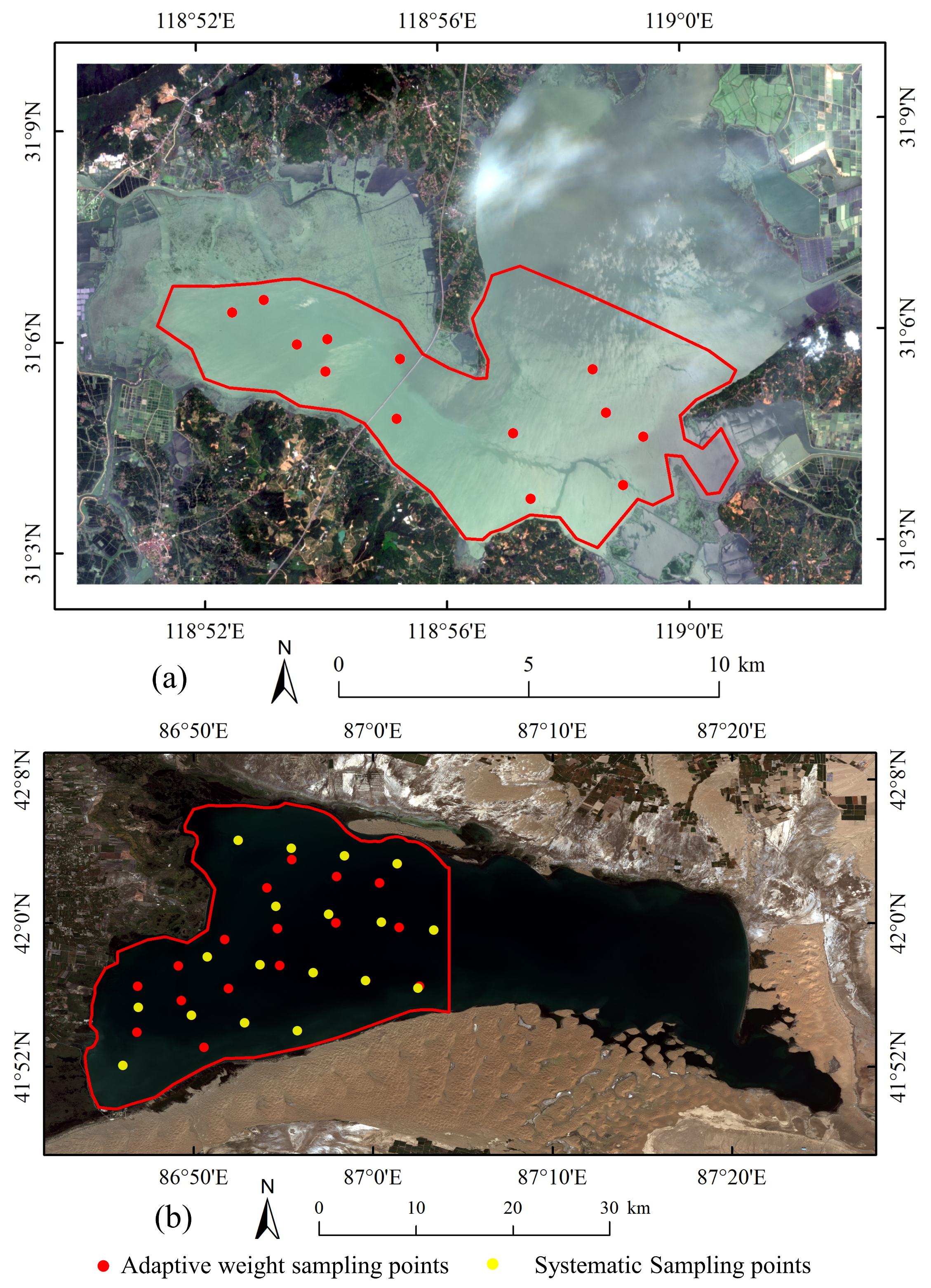
2.1. Study Area
2.2. Experimental Data
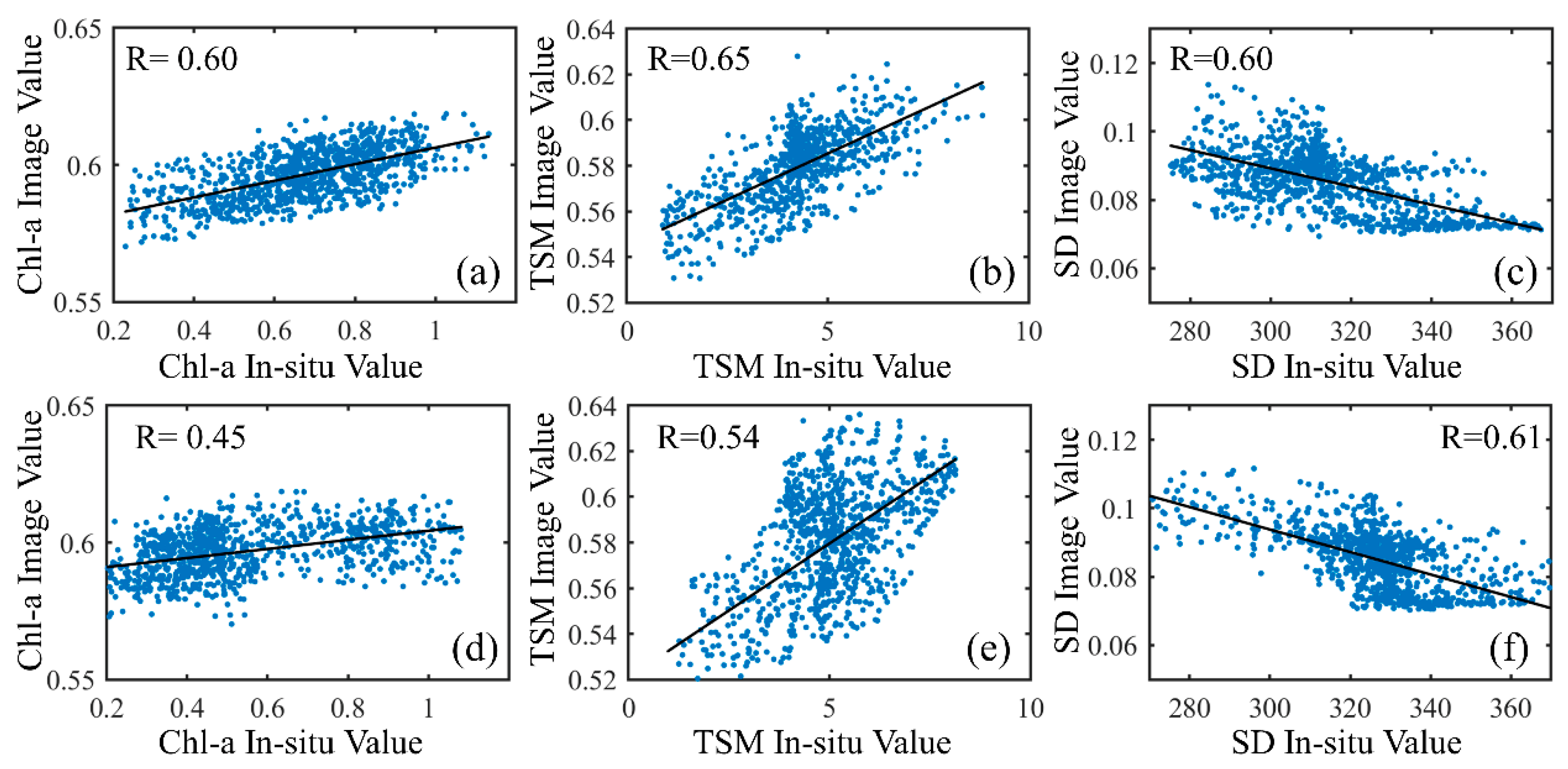
2.3. Preprocessing of Remote Sensing Dataset and In-Situ Dataset
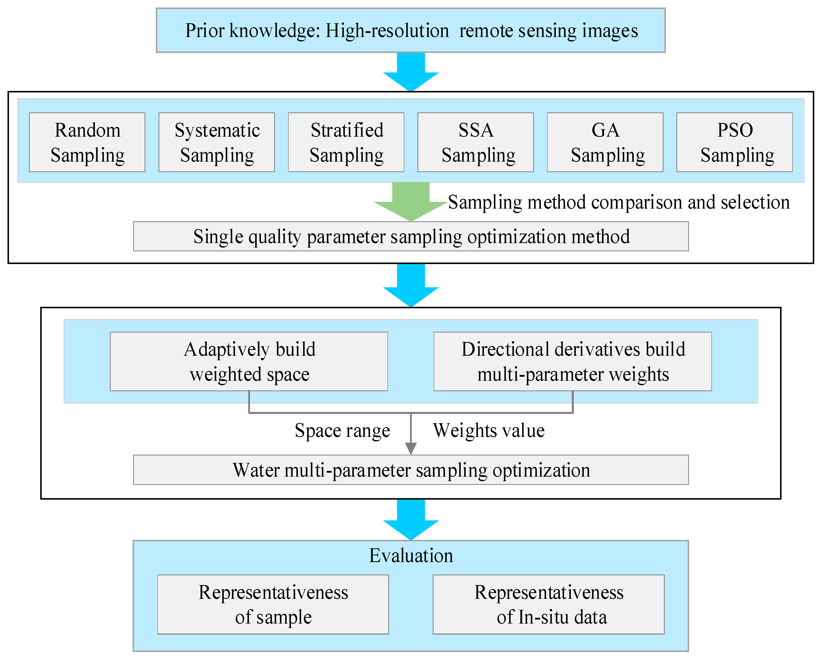
3. Method
3.1. Spatial Distribution of Water Parameters
3.2. Comparison of Water Single-Parameter Sampling Methods
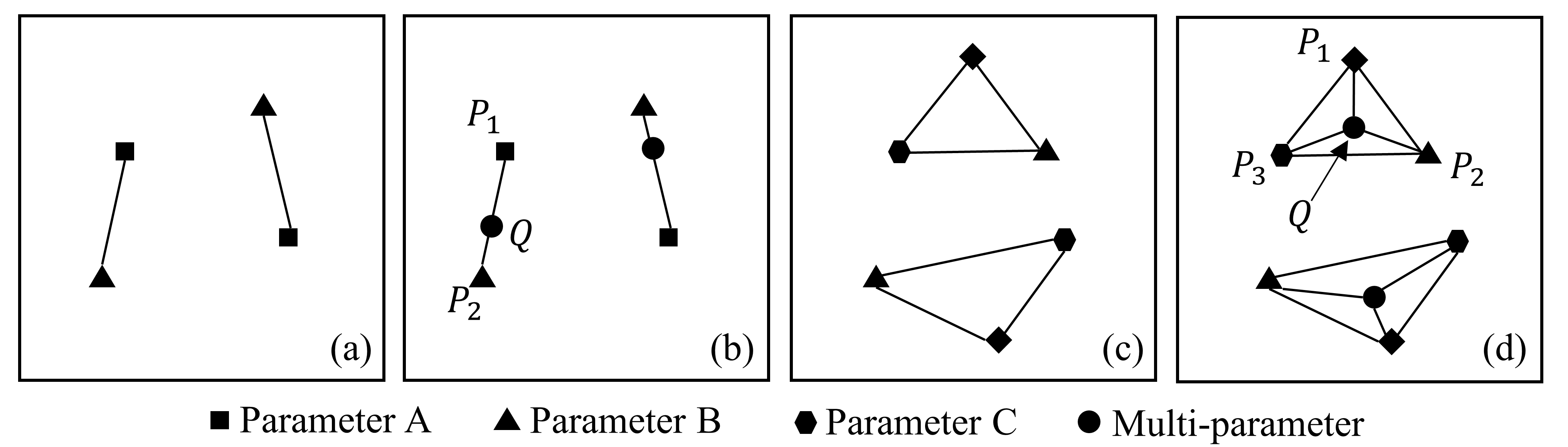
3.3. Water Multi-Parameter Sampling Method
3.4. Evaluation Method
4. Results and Analysis
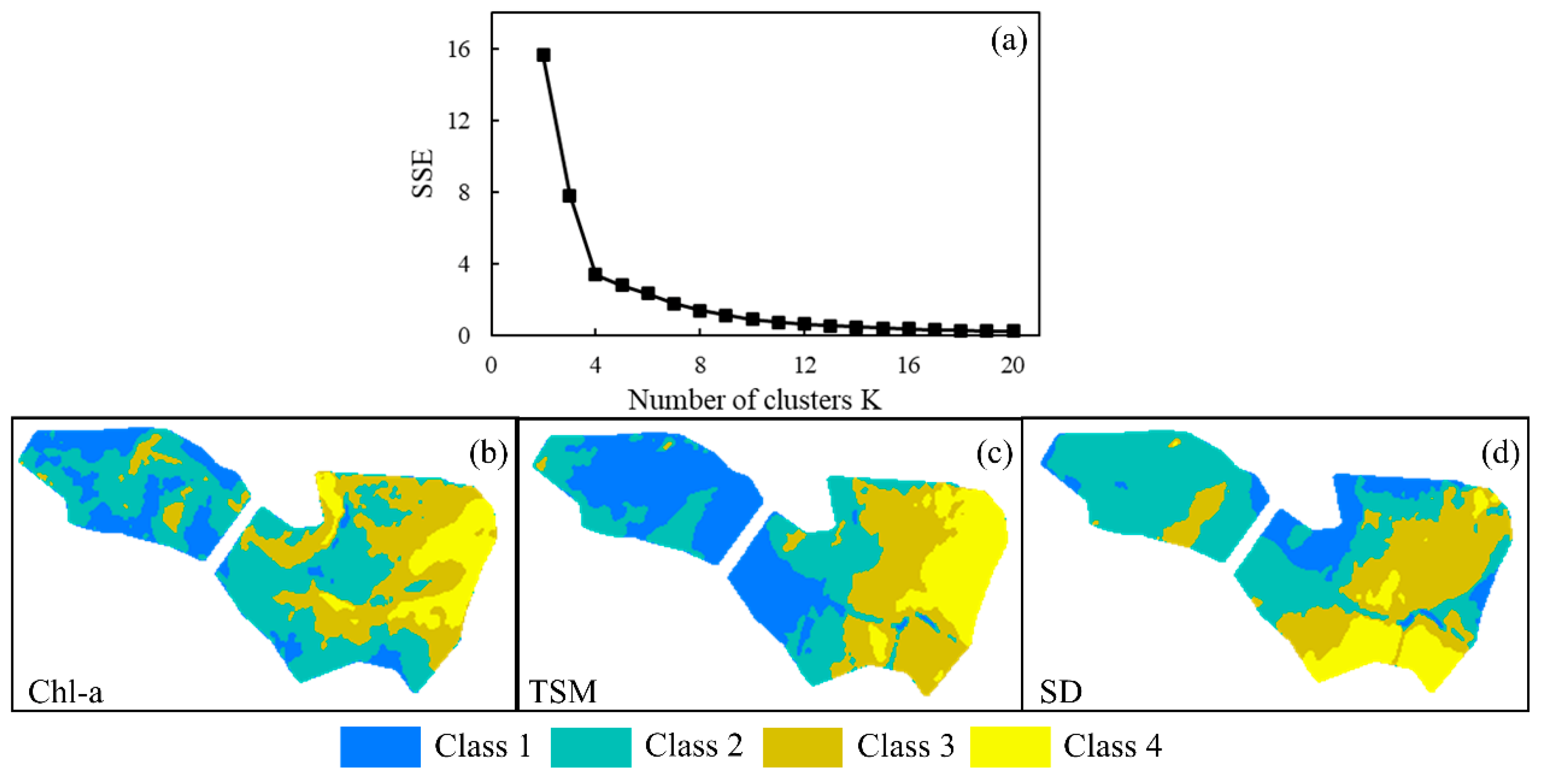
4.1. Spatial Distribution of Various Water Parameters
4.2. Effectiveness Evaluation of the Various Sampling Methods
4.2.1. Spatial Representative Comparison of Various Sampling Design Methods
4.2.2. Water Single-Parameter Sampling Points
4.3. Accuracy Evaluation of Water Multi-Parameter Sampling Method
4.4. Accuracy Evaluation of In-Situ Dataset of Water Parameters
5. Discussion
6. Conclusions
Author Contributions
Funding
Data Availability Statement
Acknowledgments
Conflicts of Interest
References
- Feng, M.; Sexton, J.O.; Channan, S.; Townshend, J.R. A global, high-resolution (30-m) inland water body dataset for 2000: First results of a topographic–spectral classification algorithm. Int. J. Digit. Earth 2016, 9, 113–133. [Google Scholar] [CrossRef] [Green Version]
- Woolway, R.I.; Kraemer, B.M.; Lenters, J.D.; Merchant, C.J.; O’Reilly, C.M.; Sharma, S. Global lake responses to climate change. Nat. Rev. Earth Environ. 2020, 1, 388–403. [Google Scholar] [CrossRef]
- Dörnhöfer, K.; Oppelt, N. Remote sensing for lake research and monitoring–Recent advances. Ecol. Indic. 2016, 64, 105–122. [Google Scholar] [CrossRef]
- Bonansea, M.; Ledesma, M.; Rodriguez, C.; Pinotti, L. Using new remote sensing satellites for assessing water quality in a reservoir. Hydrol. Sci. J. 2019, 64, 34–44. [Google Scholar] [CrossRef]
- Aires, F.; Venot, J.-P.; Massuel, S.; Gratiot, N.; Pham-Duc, B.; Prigent, C. Surface water evolution (2001–2017) at the Cambodia/Vietnam border in the upper mekong delta using satellite MODIS observations. Remote Sens. 2020, 12, 800. [Google Scholar] [CrossRef] [Green Version]
- Rai, P.K.; Chandel, R.S.; Mishra, V.N.; Singh, P. Hydrological inferences through morphometric analysis of lower Kosi river basin of India for water resource management based on remote sensing data. Appl. Water Sci. 2018, 8, 15. [Google Scholar] [CrossRef] [Green Version]
- Wang, X.; Xie, H. A review on applications of remote sensing and geographic information systems (GIS) in water resources and flood risk management. Water 2018, 10, 608. [Google Scholar] [CrossRef] [Green Version]
- Tortini, R.; Noujdina, N.; Yeo, S.; Ricko, M.; Birkett, C.M.; Khandelwal, A.; Kumar, V.; Marlier, M.E.; Lettenmaier, D.P. Satellite-based remote sensing data set of global surface water storage change from 1992 to 2018. Earth Syst. Sci. Data 2020, 12, 1141–1151. [Google Scholar] [CrossRef]
- Wang, S.; Li, J.; Zhang, W.; Cao, C.; Zhang, F.; Shen, Q.; Zhang, X.; Zhang, B. A dataset of remote-sensed Forel-Ule Index for global inland waters during 2000–2018. Sci. Data 2021, 8, 26. [Google Scholar] [CrossRef]
- Wang, X.; Yang, W. Water quality monitoring and evaluation using remote sensing techniques in China: A systematic review. Ecosyst. Health Sustain. 2019, 5, 47–56. [Google Scholar] [CrossRef] [Green Version]
- Xu, J.; Lei, S.; Bi, S.; Li, Y.; Lyu, H.; Xu, J.; Xu, X.; Mu, M.; Miao, S.; Zeng, S. Tracking spatio-temporal dynamics of POC sources in eutrophic lakes by remote sensing. Water Res. 2020, 168, 115–162. [Google Scholar] [CrossRef] [PubMed]
- Zang, W.; Lin, J.; Wang, Y.; Tao, H. Investigating small-scale water pollution with UAV remote sensing technology. In Proceedings of the World Automation Congress, Puerto Vallarta, Mexico, 24–28 June 2012; pp. 1–4. [Google Scholar]
- Feng, L.; Hou, X.; Zheng, Y. Monitoring and understanding the water transparency changes of fifty large lakes on the Yangtze Plain based on long-term MODIS observations. Remote Sens. Environ. 2019, 221, 675–686. [Google Scholar] [CrossRef]
- Palmer, S.C.; Kutser, T.; Hunter, P.D. Remote Sensing of Inland Waters: Challenges, Progress and Future Directions; Elsevier: Amsterdam, The Netherlands, 2015; pp. 1–8. [Google Scholar]
- Rui, J.; Youhua, R.; Qinhuo, L. Key methods and experiment verification for the validation of quantitative remote sensing products. Adv. Earth Sci. 2017, 6, 630–642. [Google Scholar]
- Justice, C.; Belward, A.; Morisette, J.; Lewis, P.; Privette, J.; Baret, F. Developments in the ‘validation’ of satellite sensor products for the study of the land surface. Int. J. Remote Sens. 2000, 21, 3383–3390. [Google Scholar] [CrossRef]
- Wu, X.; Xiao, Q.; Wen, J.; You, D.; Hueni, A. Advances in quantitative remote sensing product validation: Overview and current status. Earth Sci. Rev. 2019, 196, 102875. [Google Scholar] [CrossRef]
- Alilou, H.; Nia, A.M.; Keshtkar, H.; Han, D.; Bray, M. A cost-effective and efficient framework to determine water quality monitoring network locations. Sci. Total Environ. 2018, 624, 283–293. [Google Scholar] [CrossRef] [Green Version]
- Kiefer, I.; Odermatt, D.; Anneville, O.; Wüest, A.; Bouffard, D. Application of remote sensing for the optimization of in-situ sampling for monitoring of phytoplankton abundance in a large lake. Sci. Total Environ. 2015, 527, 493–506. [Google Scholar] [CrossRef]
- Hansen, C.H.; Williams, G.P.; Adjei, Z.; Barlow, A.; Nelson, E.J.; Miller, A.W. Reservoir water quality monitoring using remote sensing with seasonal models: Case study of five central-Utah reservoirs. Lake Reserv. Manag. 2015, 31, 225–240. [Google Scholar] [CrossRef]
- Noges, P.; Poikane, S.; Koiv, T.; Noges, T. Effect of chlorophyll sampling design on water quality assessment in thermally stratified lakes. Hydrobiologia 2010, 649, 157–170. [Google Scholar] [CrossRef]
- Sun, P.; Zhang, J.; Congalton, R.G.; Pan, Y.; Zhu, X. A quantitative performance comparison of paddy rice acreage estimation using stratified sampling strategies with different stratification indicators. Int. J. Digit. Earth 2018, 11, 1001–1019. [Google Scholar] [CrossRef]
- Lv, T.; Zhou, X.; Tao, Z.; Sun, X.; Wang, J.; Li, R.; Xie, F. Remote Sensing-Guided Spatial Sampling Strategy over Heterogeneous Surface Ground for Validation of Vegetation Indices Products with Medium and High Spatial Resolution. Remote Sens. 2021, 13, 2674. [Google Scholar] [CrossRef]
- Brus, D.; Knotters, M. Sampling design for compliance monitoring of surface water quality: A case study in a Polder area. Water Resour. Res. 2008, 44, W11410. [Google Scholar] [CrossRef] [Green Version]
- Ling, C.; Lu, Z. Adaptive Kriging coupled with importance sampling strategies for time-variant hybrid reliability analysis. Appl. Math. Model. 2020, 77, 1820–1841. [Google Scholar] [CrossRef]
- Vašát, R.; Heuvelink, G.; Borůvka, L. Sampling design optimization for multivariate soil mapping. Geoderma 2010, 155, 147–153. [Google Scholar] [CrossRef]
- Chen, B.; Pan, Y.; Wang, J.; Fu, Z.; Zeng, Z.; Zhou, Y.; Zhang, Y. Even sampling designs generation by efficient spatial simulated annealing. Math. Comput. Model. 2013, 58, 670–676. [Google Scholar] [CrossRef]
- Wadoux, A.M.J.C.; Brus, D.J.; Heuvelink, G.B.M. Sampling design optimization for soil mapping with random forest. Geoderma 2019, 355, 113913. [Google Scholar] [CrossRef]
- Puri, D.; Borel, K.; Vance, C.; Karthikeyan, R. Optimization of a water quality monitoring network using a spatially referenced water quality model and a genetic algorithm. Water 2017, 9, 704. [Google Scholar] [CrossRef] [Green Version]
- Cai, X.; Qiu, H.; Gao, L.; Yang, P.; Shao, X. A multi-point sampling method based on kriging for global optimization. Struct. Multidiscip. Optim. 2017, 56, 71–88. [Google Scholar] [CrossRef]
- Miralha, L.; Kim, D. Accounting for and predicting the influence of spatial autocorrelation in water quality modeling. ISPRS Int. J. Geo Inf. 2018, 7, 64. [Google Scholar] [CrossRef] [Green Version]
- Yang, X.; Jin, W. GIS-based spatial regression and prediction of water quality in river networks: A case study in Iowa. J. Environ. Manag. 2010, 91, 1943–1951. [Google Scholar] [CrossRef]
- Guedes, L.P.C.; Ribeiro, P.J., Jr.; De Stefano Piedade, S.; Uribe-Opazo, M.A. Optimization of spatial sample configurations using hybrid genetic algorithm and simulated annealing. Chil. J. Stat. 2011, 2, 39–50. [Google Scholar]
- Li, J.; Tian, L.; Wang, Y.; Jin, S.; Li, T.; Hou, X. Optimal sampling strategy of water quality monitoring at high dynamic lakes: A remote sensing and spatial simulated annealing integrated approach. Sci. Total Environ. 2021, 777, 146113. [Google Scholar] [CrossRef]
- Jiang, J.; Tang, S.; Han, D.; Fu, G.; Solomatine, D.; Zheng, Y. A comprehensive review on the design and optimization of surface water quality monitoring networks. Environ. Model. Softw. 2020, 132, 104792. [Google Scholar] [CrossRef]
- Ge, Y.; Wang, J.; Heuvelink, G.B.; Jin, R.; Li, X.; Wang, J. Sampling design optimization of a wireless sensor network for monitoring ecohydrological processes in the Babao River basin, China. Int. J. Geogr. Inf. Sci. 2015, 29, 92–110. [Google Scholar] [CrossRef]
- Rose, K.C.; Greb, S.R.; Diebel, M.; Turner, M.G. Annual precipitation regulates spatial and temporal drivers of lake water clarity. Ecol. Appl. 2017, 27, 632–643. [Google Scholar] [CrossRef] [PubMed]
- He, Y.; Gong, Z.; Zheng, Y.; Zhang, Y. Inland Reservoir Water Quality Inversion and Eutrophication Evaluation Using BP Neural Network and Remote Sensing Imagery: A Case Study of Dashahe Reservoir. Water 2021, 13, 2844. [Google Scholar] [CrossRef]
- Cheng, M.; Jiang, M.; Huang, Z.; Lei, H.; Yan, D.; Zhu, F. Research on Baiyangdian Lake Water Body Changes and Water Quality Parameters Inversion Based on Landsat Dense Time Series Data. IOP Conf. Ser. Earth Environ. Sci. 2021, 783, 012134. [Google Scholar] [CrossRef]
- Pahlevan, N.; Schott, J.R.; Franz, B.A.; Zibordi, G.; Markham, B.; Bailey, S.; Schaaf, C.B.; Ondrusek, M.; Greb, S.; Strait, C.M. Landsat 8 remote sensing reflectance (Rrs) products: Evaluations, intercomparisons, and enhancements. Remote Sens. Environ. 2017, 190, 289–301. [Google Scholar] [CrossRef]
- Li, M.-C.; Liang, S.-X.; Sun, Z.-C.; Zhang, G.-Y. Optimal Dynamic Temporal-Spatial Paramter Inversion Methods for the Marine Integrated Element Water Quality Model Using A Data-Driven Neural Network. J. Mar. Sci. Technol. 2012, 20, 13. [Google Scholar]
- Xinhui, W.; Cailan, G.; Yong, H.; Lan, L.; Zhijie, H. Spectral Feature Construction and Sensitivity Analysis of Water Quality Parameters Remote Sensing Inversion. Spectrosc. Spectr. Anal. 2021, 41, 1880–1885. [Google Scholar]
- Giardino, C.; Pepe, M.; Brivio, P.A.; Ghezzi, P.; Zilioli, E. Detecting chlorophyll, Secchi disk depth and surface temperature in a sub-alpine lake using Landsat imagery. Sci. Total Environ. 2001, 268, 19–29. [Google Scholar] [CrossRef]
- Tang, X.; Huang, M. Inversion of chlorophyll-a concentration in Donghu Lake based on machine learning algorithm. Water 2021, 13, 1179. [Google Scholar] [CrossRef]
- Cao, H.; Han, L.; Li, W.; Liu, Z.; Li, L. Inversion and distribution of total suspended matter in water based on remote sensing images—A case study on Yuqiao Reservoir, China. Water Environ. Res. 2021, 93, 582–595. [Google Scholar] [CrossRef] [PubMed]
- Dall’Olmo, G.; Gitelson, A.A. Effect of bio-optical parameter variability on the remote estimation of chlorophyll-a concentration in turbid productive waters: Experimental results. Appl. Opt. 2005, 44, 412–422. [Google Scholar] [CrossRef] [Green Version]
- Alizadeh, M.J.; Jafari Nodoushan, E.; Kalarestaghi, N.; Chau, K.W. Toward multi-day-ahead forecasting of suspended sediment concentration using ensemble models. Environ. Sci. Pollut. Res. 2017, 24, 28017–28025. [Google Scholar] [CrossRef]
- Blömer, J.; Lammersen, C.; Schmidt, M.; Sohler, C. Theoretical analysis of the k-means algorithm—A survey. In Algorithm Engineering; Springer: Berlin/Heidelberg, Germany, 2016; pp. 81–116. [Google Scholar]
- Su, T.; Dy, J. A deterministic method for initializing k-means clustering. In Proceedings of the 16th IEEE International Conference on Tools with Artificial Intelligence, Boca Raton, FL, USA, 15–17 November 2004; pp. 784–786. [Google Scholar]
- Nainggolan, R.; Perangin-angin, R.; Simarmata, E.; Tarigan, A.F. Improved the performance of the K-means cluster using the sum of squared error (SSE) optimized by using the elbow method. In Proceedings of the 1st International Conference of SNIKOM 2018, Medan, Indonesia, 23–24 November 2018; IOP Publishing: Bristol, UK; Volume 1361, p. 012015. [Google Scholar]
- Fuhg, J.N.; Fau, A.; Nackenhorst, U. State-of-the-art and comparative review of adaptive sampling methods for kriging. Arch. Comput. Methods Eng. 2021, 28, 2689–2747. [Google Scholar] [CrossRef]
- Oliver, M.A.; Webster, R. Kriging: A method of interpolation for geographical information systems. Int. J. Geogr. Inf. Syst. 1990, 4, 313–332. [Google Scholar] [CrossRef]
- Brus, D.; Kempen, B.; Heuvelink, G. Sampling for validation of digital soil maps. Eur. J. Soil Sci. 2011, 62, 394–407. [Google Scholar] [CrossRef]
- Shao, S.; Zhang, H.; Fan, M.; Su, B.; Wu, J.; Zhang, M.; Yang, L.; Gao, C. Spatial variability-based sample size allocation for stratified sampling. Catena 2021, 206, 105509. [Google Scholar] [CrossRef]
- Bartolucci, A.A.; Bartolucci, A.; Bae, S.; Singh, K.P. A Bayesian method for computing sample size and cost requirements for stratified random sampling of pond water. Environ. Model. Softw. 2006, 21, 1319–1323. [Google Scholar] [CrossRef]
- Hyun, S.-Y.; Seo, Y.I. The systematic sampling for inferring the survey indices of Korean groundfish stocks. Fish. Aquat. Sci. 2018, 21, 24. [Google Scholar] [CrossRef]
- Liyanage, C.P.; Marasinghe, A.; Yamada, K. Comparison of optimized selection methods of sampling sites network for water quality monitoring in a river. Int. J. Affect. Eng. 2016, 15, 195–204. [Google Scholar] [CrossRef] [Green Version]
- Yang, L.; Zhao, X.; Peng, S.; Li, X. Water quality assessment analysis by using combination of Bayesian and genetic algorithm approach in an urban lake, China. Ecol. Model. 2016, 339, 77–88. [Google Scholar] [CrossRef]
- Wang, J.; Ge, Y.; Heuvelink, G.B.; Zhou, C. Spatial sampling design for estimating regional GPP with spatial heterogeneities. IEEE Geosci. Remote Sens. Lett. 2013, 11, 539–543. [Google Scholar] [CrossRef]
- Amine, K. Multiobjective simulated annealing: Principles and algorithm variants. Adv. Oper. Res. 2019, 2019, 1–13. [Google Scholar] [CrossRef]
- Jahandideh-Tehrani, M.; Bozorg-Haddad, O.; Loáiciga, H.A. Application of particle swarm optimization to water management: An introduction and overview. Environ. Monit. Assess. 2020, 192, 281. [Google Scholar] [CrossRef]
- Ding, P. The Integral of Second-order Directional Derivative. arXiv 2021, arXiv:2107.11038. [Google Scholar]
- Meng, Q.; Liu, Z.; Borders, B.E. Assessment of regression kriging for spatial interpolation–comparisons of seven GIS interpolation methods. Cartogr. Geogr. Inf. Sci. 2013, 40, 28–39. [Google Scholar] [CrossRef]
- Myers, L.; Sirois, M.J. Spearman correlation coefficients, differences between. Encycl. Stat. Sci. 2004, 12. [Google Scholar] [CrossRef]
- Jose, V.R.R. Percentage and relative error measures in forecast evaluation. Oper. Res. 2017, 65, 200–211. [Google Scholar] [CrossRef]
- Yanlai, Z. Real-time probabilistic forecasting of river water quality under data missing situation: Deep learning plus post-processing techniques. J. Hydrol. 2020, 589, 125–164. [Google Scholar]


| Lake | Purpose | Satellite Image Date | In-Situ Data |
|---|---|---|---|
| Nanyi Lake | Sampling design | Time: 28 August 2021 Satellite: Sentinel-2 | Time: 31 August 2021 Water parameters: Chl-a, TSM, SD |
| Validation | Time: 31 August 2021 Satellite: GF-6 | ||
| Bosten Lake | Sampling design | Time: 10 September 2021 Satellite: GF-1 | Time: 14 September 2021 Water parameters: Chl-a, TSM, SD |
| Validation | Time: 15 September 2021 Satellite: GF-1B |
| Lake | Parameter | Maximum | Minimum | Average | Standard Deviation |
|---|---|---|---|---|---|
| Nanyi Lake | Chl-a | 2.23 | 0.71 | 1.39 | 0.46 |
| TSM | 16 | 4 | 9.60 | 3.59 | |
| SD | 125 | 82 | 104.60 | 11.10 | |
| Bosten Lake | Chl-a | 1.12 | 0.23 | 0.63 | 0.26 |
| TSM | 9 | 1 | 5.28 | 2.20 | |
| SD | 366 | 240 | 309.97 | 26.62 |
| Sampling Method | Objective Function | Theory |
|---|---|---|
| random sampling | Null | Select the sample points by random number [53] |
| stratified sampling | Divide the study area into sub-areas and use random sampling within each sub-area [24,54,55] | |
| systematic sampling | Select the sample points by using a regular grid [24,56] | |
| GA sampling | The objective function is minimized by genetic operations, such as selection, crossover, and variation of different initial sampling points [57,58] | |
| SSA sampling | The objective function is minimized by allocating sampling locations randomly [36,59,60] | |
| PSO sampling | The objective function is to minimize collaboration and information sharing among individuals in the group [61] |
| RMSE | Spatial Distribution Map of the Three Parameters | ||
|---|---|---|---|
| Chl-a | TSM | SD | |
| Chl-a sampling points | 0.0128 | 0.0227 | 0.0081 |
| TSM sampling points | 0.0241 | 0.0196 | 0.0067 |
| SD sampling points | 0.0236 | 0.0267 | 0.0060 |
| Adaptive weight sampling points | 0.0156 | 0.0216 | 0.0065 |
Publisher’s Note: MDPI stays neutral with regard to jurisdictional claims in published maps and institutional affiliations. |
© 2022 by the authors. Licensee MDPI, Basel, Switzerland. This article is an open access article distributed under the terms and conditions of the Creative Commons Attribution (CC BY) license (https://creativecommons.org/licenses/by/4.0/).
Share and Cite
Zhai, M.; Tao, Z.; Zhou, X.; Lv, T.; Wang, J.; Li, R. Water Multi-Parameter Sampling Design Method Based on Adaptive Sample Points Fusion in Weighted Space. Remote Sens. 2022, 14, 2780. https://doi.org/10.3390/rs14122780
Zhai M, Tao Z, Zhou X, Lv T, Wang J, Li R. Water Multi-Parameter Sampling Design Method Based on Adaptive Sample Points Fusion in Weighted Space. Remote Sensing. 2022; 14(12):2780. https://doi.org/10.3390/rs14122780
Chicago/Turabian StyleZhai, Mingjian, Zui Tao, Xiang Zhou, Tingting Lv, Jin Wang, and Ruoxi Li. 2022. "Water Multi-Parameter Sampling Design Method Based on Adaptive Sample Points Fusion in Weighted Space" Remote Sensing 14, no. 12: 2780. https://doi.org/10.3390/rs14122780
APA StyleZhai, M., Tao, Z., Zhou, X., Lv, T., Wang, J., & Li, R. (2022). Water Multi-Parameter Sampling Design Method Based on Adaptive Sample Points Fusion in Weighted Space. Remote Sensing, 14(12), 2780. https://doi.org/10.3390/rs14122780