
Spatial and Temporal Distributions of Ionospheric Irregularities Derived from Regional and Global ROTI Maps

 ,
,  ,
,
Abstract
:
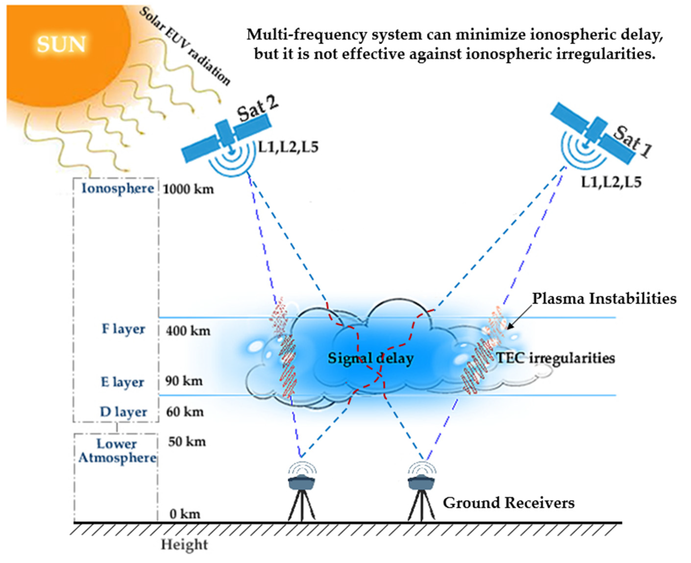
1. Introduction
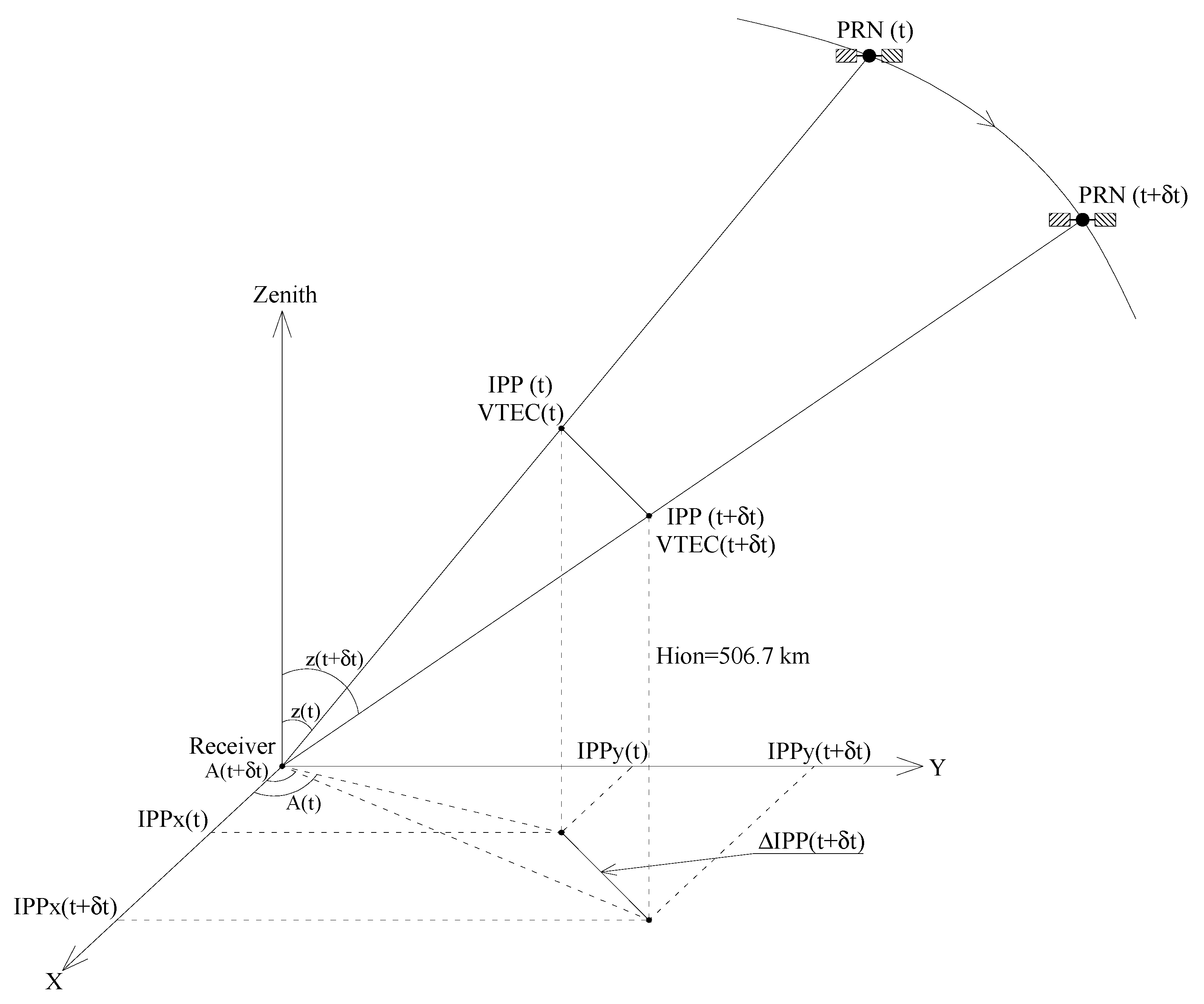
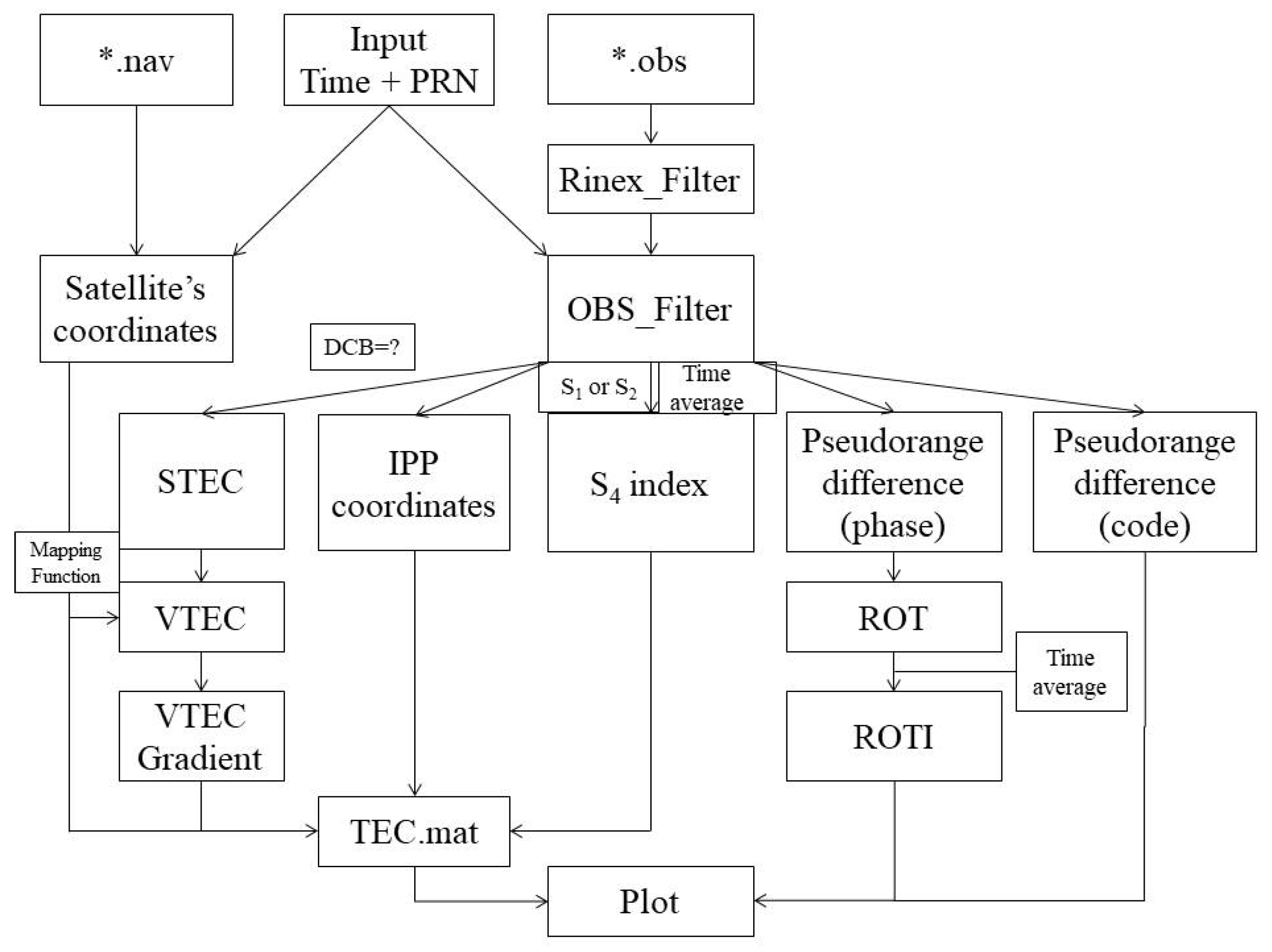
2. Data and Method
- Filter observations from the RINEX files: The observations are rearranged following the observed satellite and epoch, after which the data are collected according to the selected satellite and time;
- The coordinates of the selected satellite during the selected time from the navigation file are calculated;
- The user chooses whether or not to smooth the pseudo range and which observation will be used (P1, P2, or C1, C2);
- STEC is converted to VTEC and the VTEC gradient is calculated to check the possible rapid fluctuations in VTEC results;
- The IPP coordinates are computed and stored;
- The differences in pseudo-ranges derived from code and phase measurements are calculated and compared to detect the incidental cycle slip error in the phase measurements;
- ROT and ROTI are determined following Equations (1)–(4). For ROTI computation, the calculation time interval must be set up. In our research, this value is chosen as five minutes, as discussed before;
- All the results are stored in *.MAT files and can be used later for other purposes. Based on the variations in the VTEC gradient, S4, ROT, and ROTI values, the levels of scintillations can be estimated and the correlations between ionospheric scintillations and the changes in VTEC can be explored.

3. Results
3.1. Ionospheric Irregularity Observations Using ROT and ROTI Indices
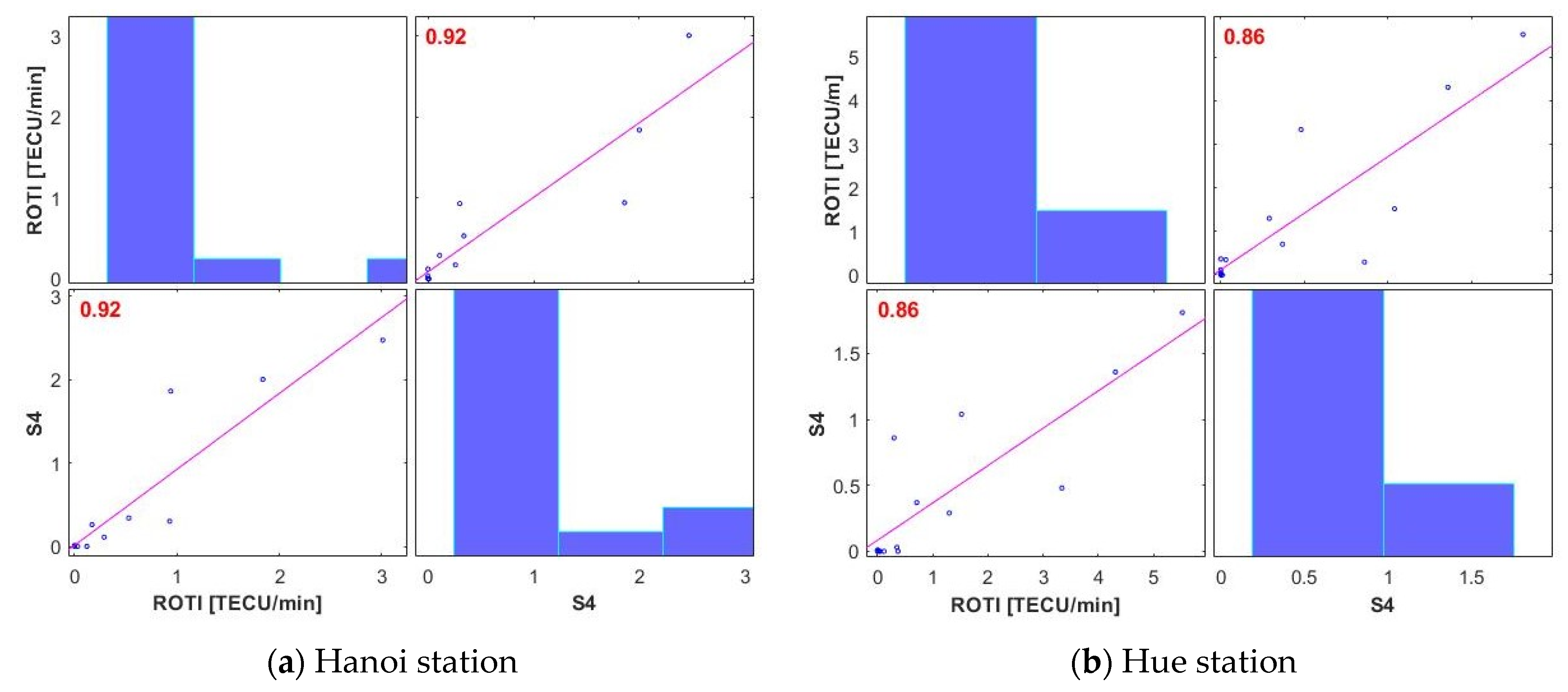
3.1.1. Use of S4 Index to Validate the ROTI Results and Their Correlation
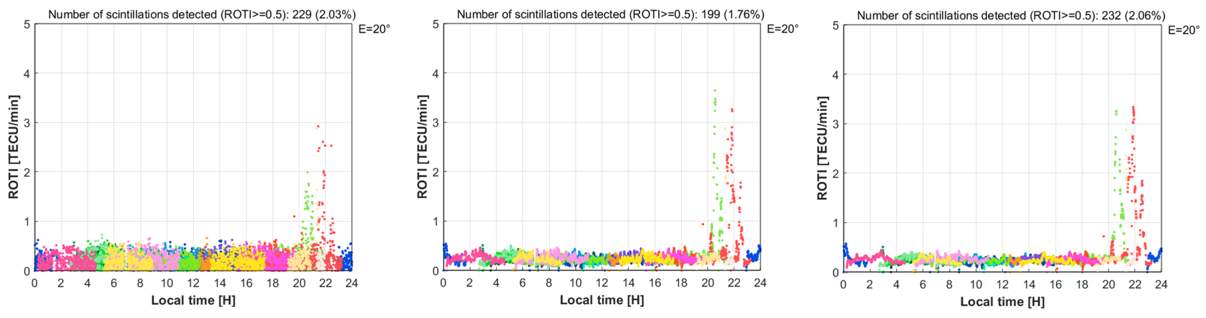
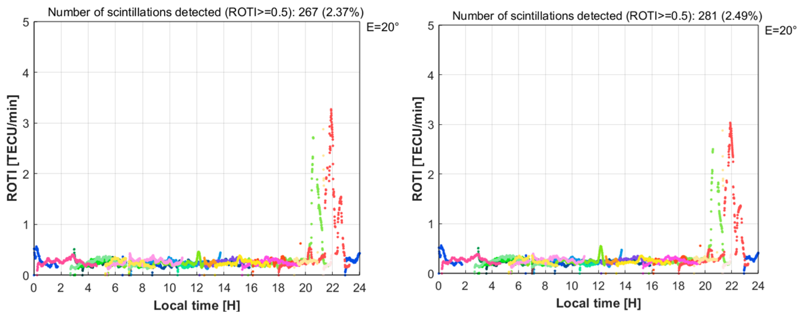
3.1.2. Reasonable Choices of Satellite Elevation Threshold and Time Span of ROTI Calculation
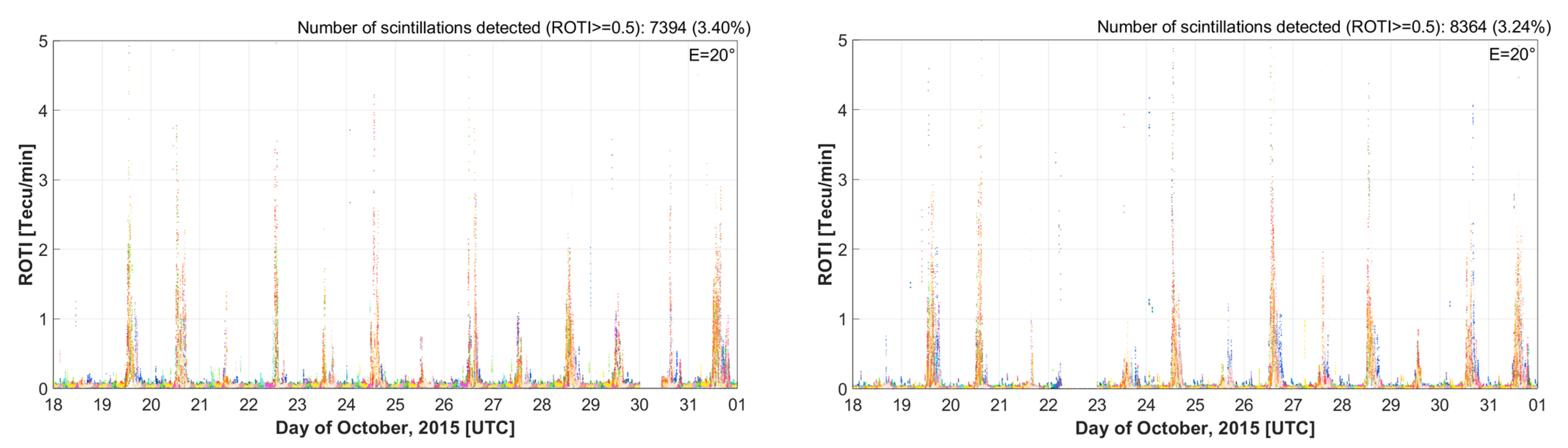
3.1.3. Ionospheric Disturbances in the Southeast Asia Region during the Second Half of March and October 2015
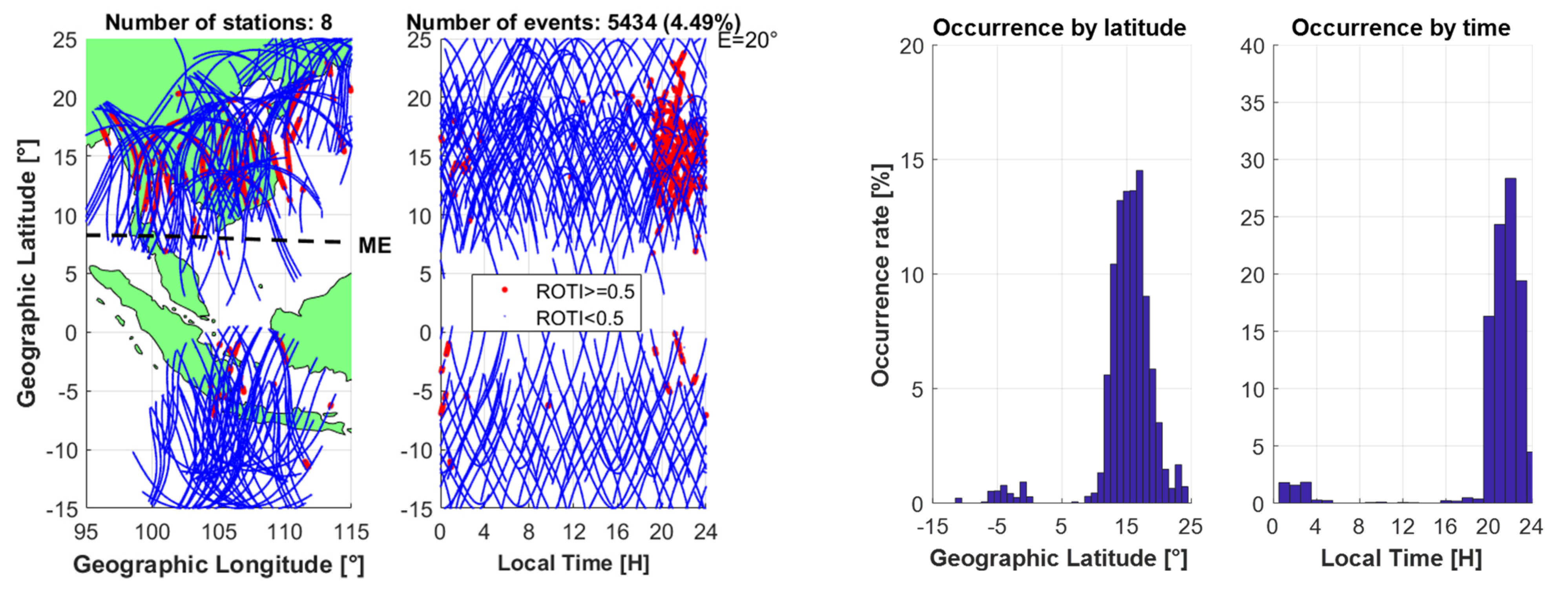
3.2. Regional Ionospheric Irregularity Maps for Southeast Asia
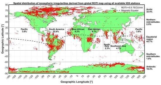
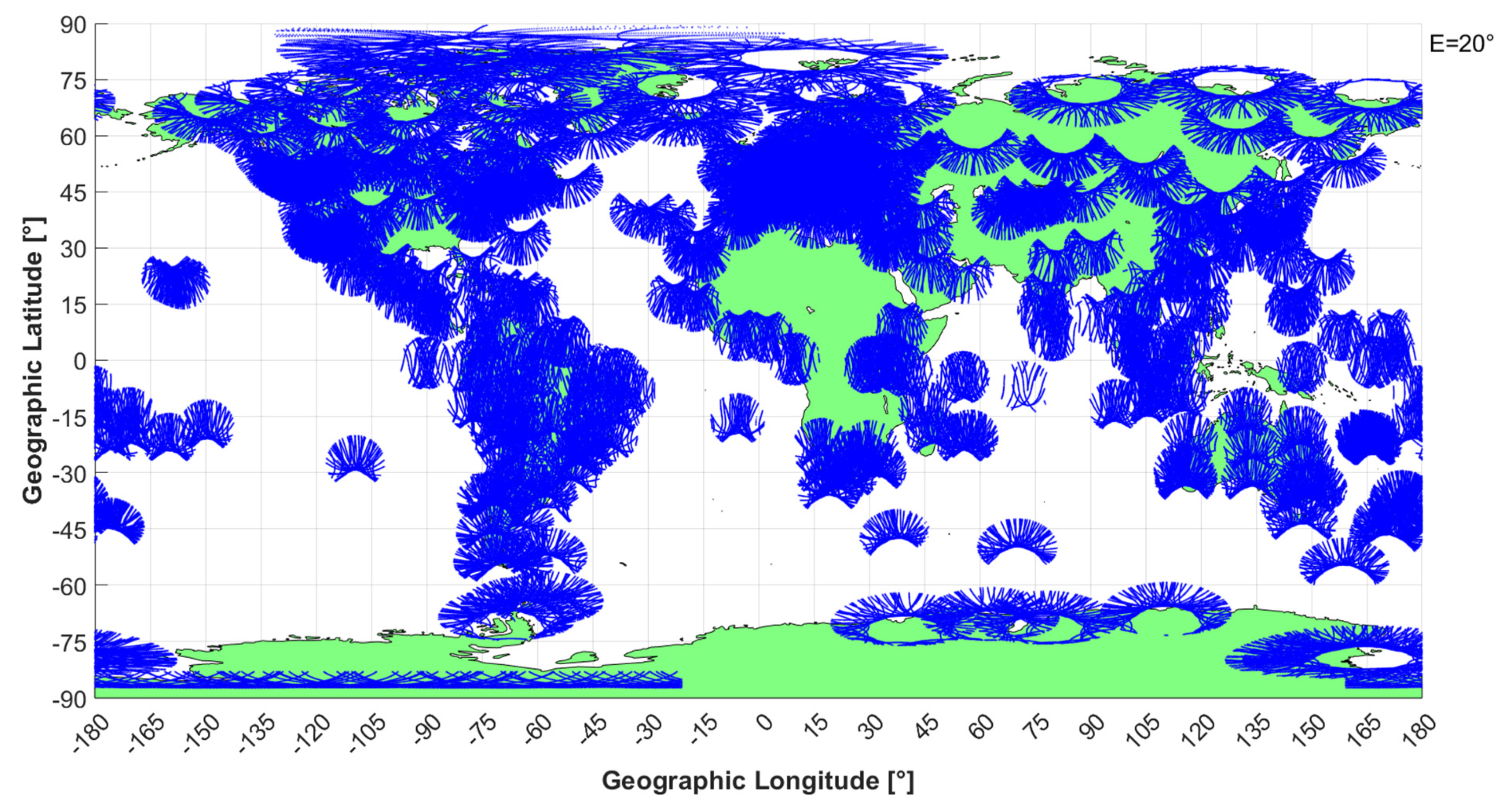
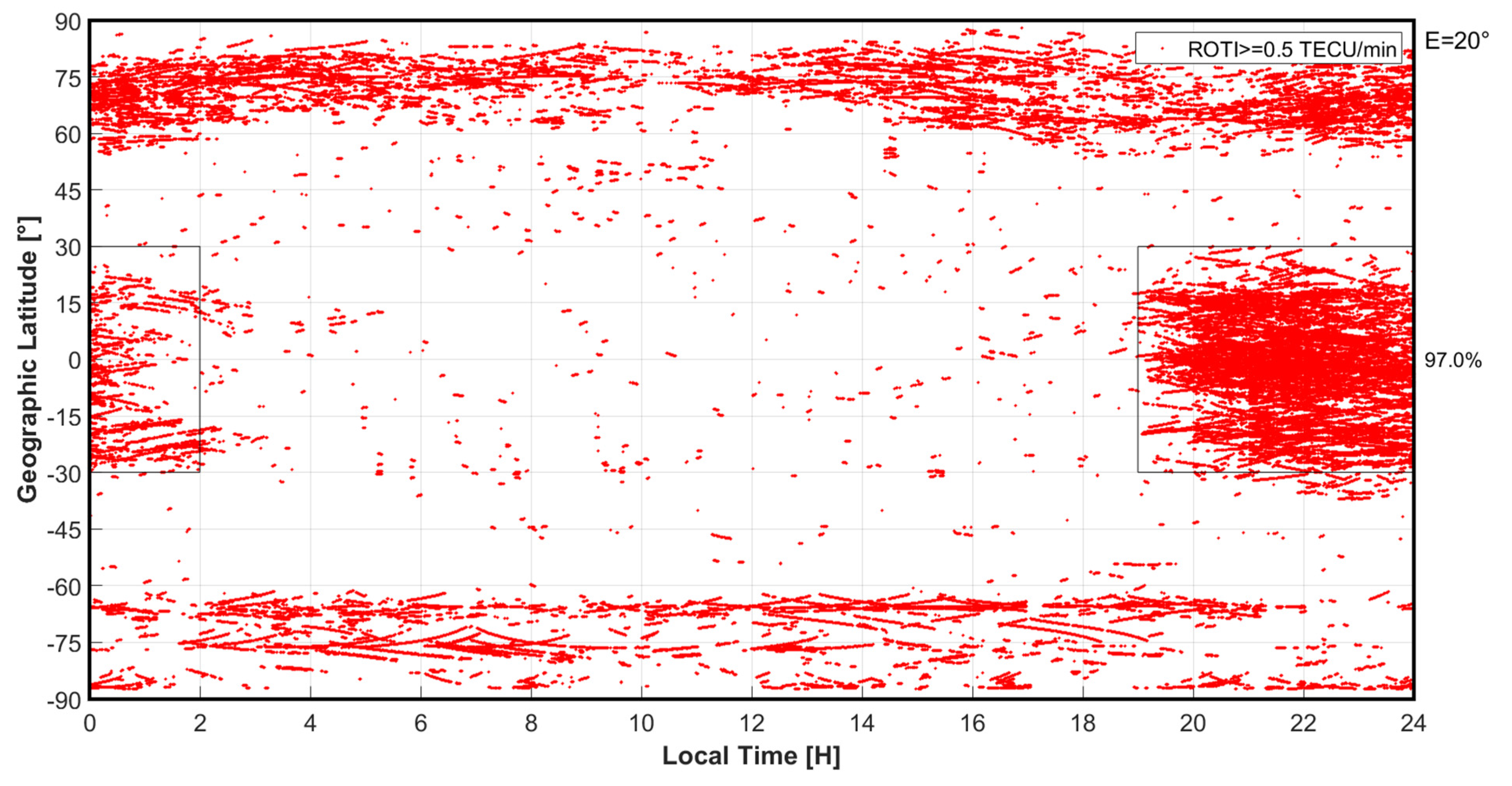
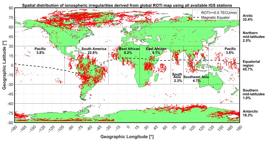
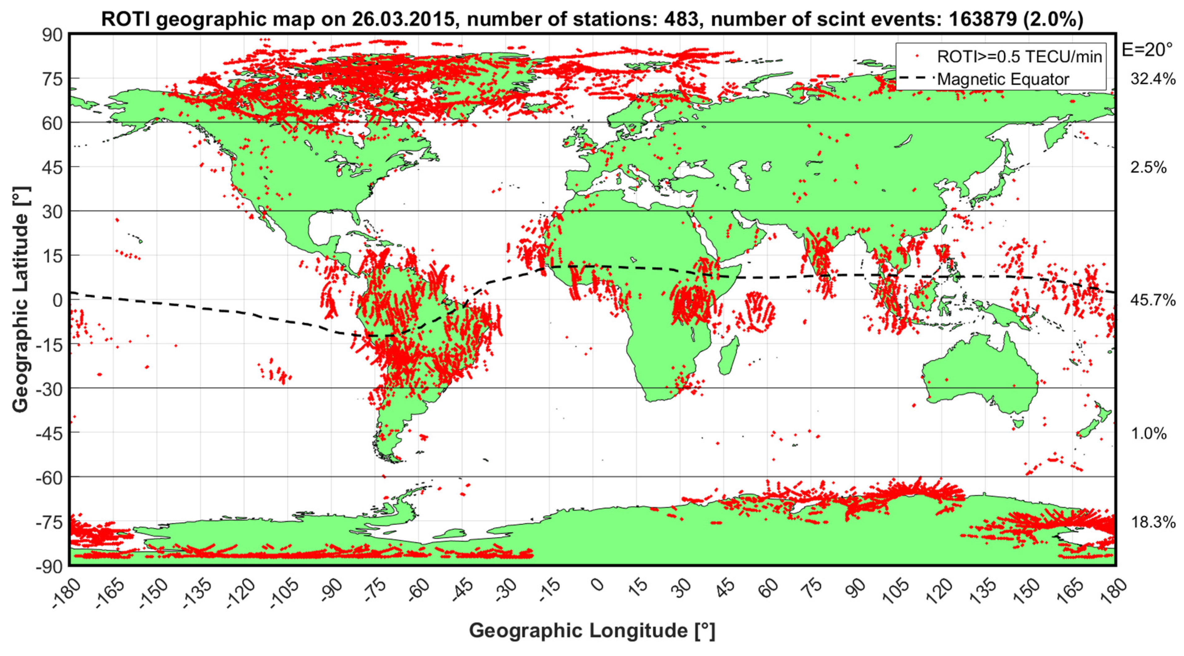
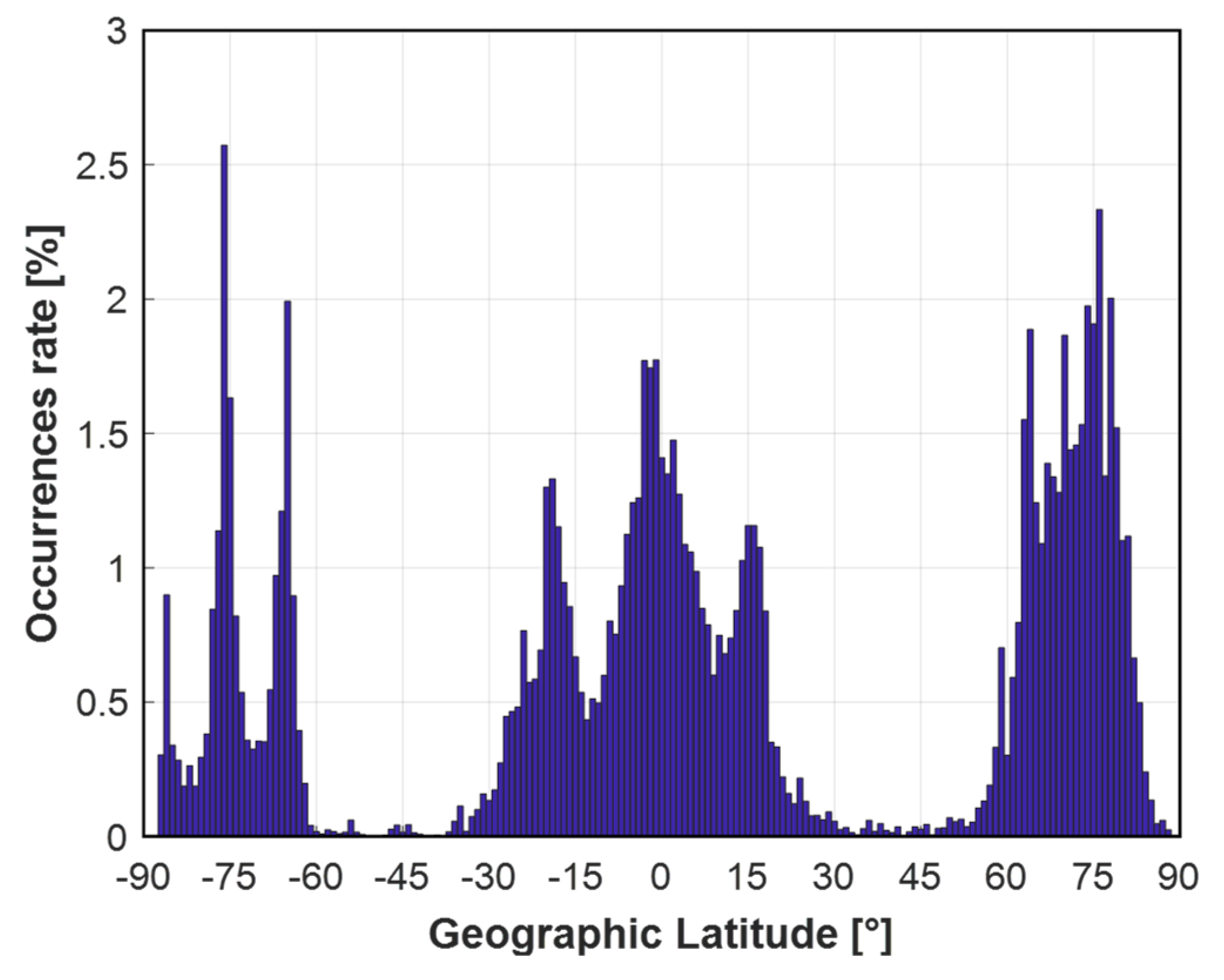
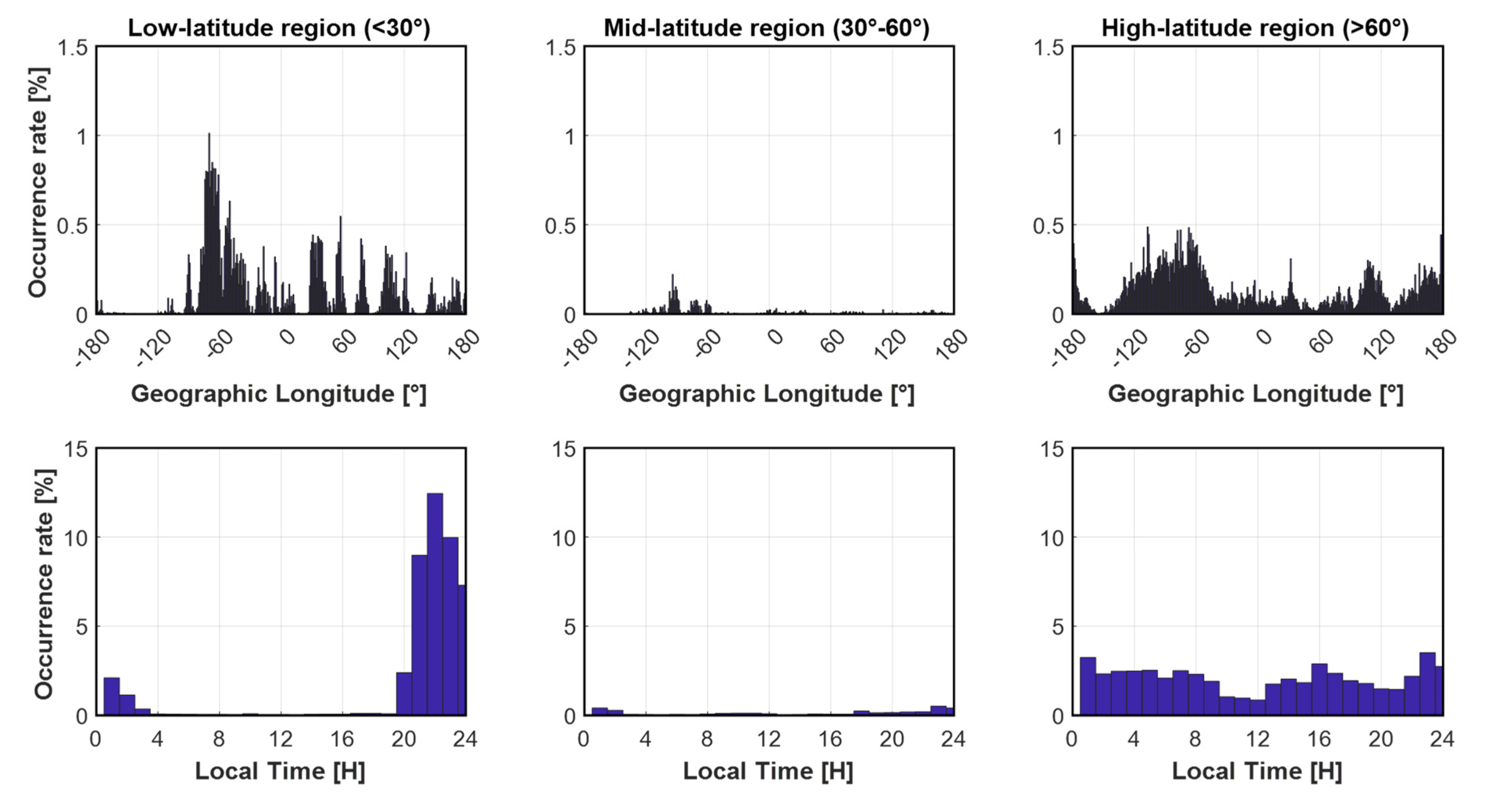
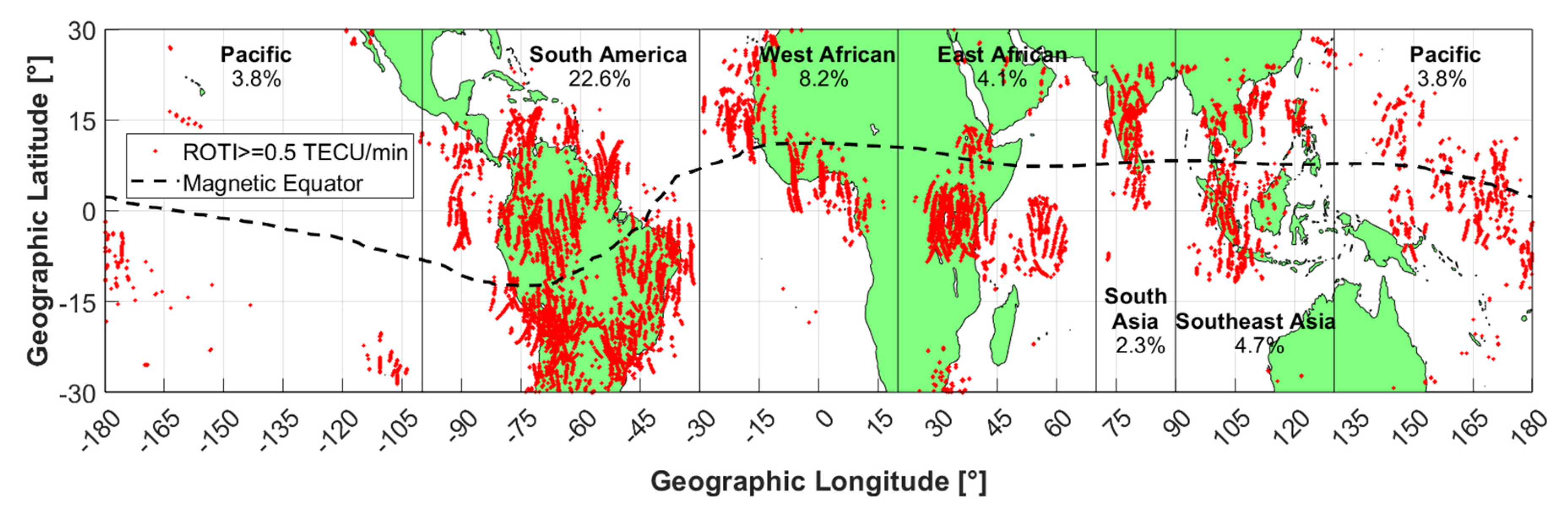
3.3. Global Ionospheric Irregularity Maps
4. Discussion
5. Conclusions
Author Contributions
Funding
Informed Consent Statement
Data Availability Statement
Acknowledgments
Conflicts of Interest
References
- Oluwadare, T.S.; Thai, C.N.; Akala, A.O.-O.; Heise, S.; Alizadeh, M.; Schuh, H. Characterization of GPS-TEC over African equatorial ionization anomaly (EIA) region during 2009–2016. Adv. Space Res. 2018, 63, 282–301. [Google Scholar] [CrossRef]
- Alizadeh, M.M.; Wijaya, D.; Hobiger, T.; Weber, R.; Schuh, H. Ionospheric effects on microwave signals. In Atmospheric Effects in Space Geodesy; Böhm, J., Schuh, H., Eds.; Springer: Berlin/Heidelberg, Germany, 2013; ISBN 978-3-642-36931-5. [Google Scholar]
- Klobuchar, J.A. Ionospheric Time-Delay algorithm for single-frequency 803 GPS users. IEEE Trans. Aerosp. Electron. Syst. 1987, 23, 325–331. [Google Scholar] [CrossRef]
- Aragon-Angel, A.; Zürn, M.; Rovira-Garcia, A. Galileo ionospheric correction algorithm: An optimization study of NeQuick-G. Radio Sci. 2019, 54, 1156–1169. [Google Scholar] [CrossRef]
- Yuan, Y.; Wang, N.; Li, Z.; Huo, X. The BeiDou Global Broadcast Ionospheric Delay Correction Model (BDGIM) and Its Preliminary Performance Evaluation Results. Navigation 2019, 66, 55–69. [Google Scholar] [CrossRef] [Green Version]
- Su, K.; Jin, S.; Hoque, M.M. Evaluation of Ionospheric Delay Effects on Multi-GNSS Positioning Performance. Remote Sens. 2019, 11, 171. [Google Scholar] [CrossRef] [Green Version]
- Aol, S.; Buchert, S.; Jurua, E. Ionospheric irregularities and scintillations: A direct comparison of in situ density observations with ground-based L-band receivers. Earth Planets Space 2020, 72, 1–15. [Google Scholar] [CrossRef]
- Nguyen, T.C. Use of the East Asia GPS Receiving Network to Observe Ionospheric VTEC Variations, Scintillation and EIA Features during the Solar Cycle 24. Ph.D. Thesis, Technische Universität Berlin, Berlin, Germany, 2021. [Google Scholar] [CrossRef]
- Aarons, J. Equatorial scintillations: A review. IEEE Trans. Antennas Propag. 1977, 25, 729–736. [Google Scholar] [CrossRef]
- Abadi, P.; Saito, S.; Srigutomo, W. Low-latitude scintillation occurrences around the equatorial anomaly crest over Indonesia. Ann. Geophys. 2014, 32, 7–17. [Google Scholar] [CrossRef] [Green Version]
- Polekh, N.; Zolotukhina, N.; Kurkin, V.; Zherebtsov, G.; Shi, J.; Wang, G.; Wang, Z. Dynamics of ionospheric disturbances during the 17–19 March 2015 geomagnetic storm over East Asia. Adv. Space Res. 2017, 60, 2464–2476. [Google Scholar] [CrossRef]
- Alfonsi, L.; Wernik, A.; Materassi, M.; Spogli, L. Modelling ionospheric scintillation under the crest of the equatorial anomaly. Adv. Space Res. 2017, 60, 1698–1707. [Google Scholar] [CrossRef]
- McCaffrey, A.M.; Jayachandran, P.T. Determination of the Refractive Contribution to GPS Phase “Scintillation”. J. Geophys. Res. Space Phys. 2019, 124, 1454–1469. [Google Scholar] [CrossRef]
- Bhattacharyya, A.; Beach, T.L.; Basu, S.; Kintner, P.M. Nighttime equatorial ionosphere: GPS scintillations and differential carrier phase fluctuations. Radio Sci. 2000, 35, 209–224. [Google Scholar] [CrossRef]
- Cervera, M.A.; Thomas, R.M. Latitudinal and temporal variation of equatorial ionospheric irregularities determined from GPS scintillation observations. Ann. Geophys. 2006, 24, 3329–3341. [Google Scholar] [CrossRef]
- Spogli, L.; Alfonsi, L.; De Franceschi, G.; Romano, V.; Aquino, M.H.O.; Dodson, A. Climatology of GPS ionospheric scintillations over high and mid-latitude European regions. Ann. Geophys. 2009, 27, 3429–3437. [Google Scholar] [CrossRef]
- Nguyen, V.K.; Rovira-Garcia, A.; Juan, J.M.; Sanz, J.; González-Casado, G.; La, T.V.; Ta, T.H. Measuring phase scintillation at different frequencies with conventional GNSS receivers operating at 1 Hz. J. Geod. 2019, 93, 1985–2001. [Google Scholar] [CrossRef] [Green Version]
- Pi, X.; Mannucci, A.J.; Lindqwister, U.J.; Ho, C.M. Monitoring of global ionospheric irregularities using the Worldwide GPS Network. Geophys. Res. Lett. 1997, 24, 2283–2286. [Google Scholar] [CrossRef]
- Basu, S.; Groves, K.; Quinn, J.; Doherty, P. A comparison of TEC fluctuations and scintillations at Ascension Island. J. Atmos. Sol. -Terr. Phys. 1999, 61, 1219–1226. [Google Scholar] [CrossRef]
- Beach, T.L.; Kintner, P.M. Simultaneous Global Positioning System observations of equatorial scintillations and total electron content fluctuations. J. Geophys. Res. Space Phys. 1999, 104, 22553–22565. [Google Scholar] [CrossRef]
- Yuan, Y.; Ou, J. Auto-covariance estimation of variable samples (ACEVS) and its application for monitoring random ionospheric disturbances using GPS. J. Geod. 2001, 75, 438–447. [Google Scholar] [CrossRef]
- SBAS Ionospheric Working Group. Effect of Ionospheric Scintillations on GNSS–A White Paper; Stanford University: Stanford, CA, USA, 2010; pp. 2–11. [Google Scholar]
- Stolle, C.; Manoj, C.; Lühr, H.; Maus, S.; Alken, P. Estimating the daytime Equatorial Ionization Anomaly strength from electric field proxies. J. Geophys. Res. Space Phys. 2008, 113. [Google Scholar] [CrossRef]
- Guo, K.; Veettil, S.V.; Weaver, B.J.; Aquino, M. Mitigating high latitude ionospheric scintillation effects on GNSS Precise Point Positioning exploiting 1-s scintillation indices. J. Geod. 2021, 95, 30. [Google Scholar] [CrossRef]
- Wu, C.-C.; Liou, K.; Lepping, R.P.; Hutting, L.; Plunkett, S.; Howard, R.A.; Socker, D. The first super geomagnetic storm of solar cycle 24: “The St. Patrick’s day event (17 March 2015)”. Earth Planets Space 2016, 68, 151. [Google Scholar] [CrossRef] [Green Version]
- Shinagawa, H.; Jin, H.; Miyoshi, Y.; Fujiwara, H.; Yokoyama, T.; Otsuka, Y. Daily and seasonal variations in the linear growth rate of the Rayleigh-Taylor instability in the ionosphere obtained with GAIA. Prog. Earth Planet. Sci. 2018, 5, 16. [Google Scholar] [CrossRef]
- Jacobsen, K.S. The impact of different sampling rates and calculation time intervals on ROTI values. J. Space Weather. Space Clim. 2014, 4, A33. [Google Scholar] [CrossRef] [Green Version]
- Ma, G.; Maruyama, T. A super bubble detected by dense GPS network at east Asian longitudes. Geophys. Res. Lett. 2006, 33. [Google Scholar] [CrossRef]
- Zou, Y.; Wang, D. A study of GPS ionospheric scintillations observed at Guilin. J. Atmos. Sol.-Terr. Phys. 2009, 71, 1948–1958. [Google Scholar] [CrossRef]
- Yang, Z.; Liu, Z. Correlation between ROTI and Ionospheric Scintillation Indices using Hong Kong low-latitude GPS data. GPS Solut. 2015, 20, 815–824. [Google Scholar] [CrossRef]
- Abhakara, P. Ionospheric Irregularities as Observed from the GPS Reference Station in Singapore; Master of Electrical Engineering Program, Cornell University: New York, NY, USA, 2004. [Google Scholar]
- Jiyun, L.; Pullen, S.; Datta-Barua, S.; Enge, P. Assessment of Nomial Ionosphere Spatial Decorrelation for LASS. In Proceedings of the IEEE/ION PLANS, San Diego, CA, USA, 25–27 April 2006; pp. 506–514. [Google Scholar]
- Anderson, D.N. Forecasting the occurrence of ionospheric scintillation activity in the equatorial ionosphere on a day-to-day basis. GPS Solut. 2003, 7, 200–202. [Google Scholar] [CrossRef]
- Beniguel, Y.; Hamel, P. A global ionosphere scintillation propagation model for equatorial regions. J. Space Weather. Space Clim. 2011, 1, A04. [Google Scholar] [CrossRef]
- Guo, K.; Aquino, M.; Veettil, S.V. Ionospheric scintillation intensity fading characteristics and GPS receiver tracking performance at low latitudes. GPS Solut. 2019, 23, 43. [Google Scholar] [CrossRef] [Green Version]
- Huang, L.; Wang, J.; Jiang, Y.; Chen, Z.; Zhao, K. A study of GPS ionospheric scintillations observed at Shenzhen. Adv. Space Res. 2014, 54, 2208–2217. [Google Scholar] [CrossRef]
- Le, H.M.; Tran, T.L.; Amory-Mazaudier, C.; Fleury, R.; Bourdillon, A.; Hu, J.; Vu, T.H.; Nguyen, C.T.; Le, T.T.; Nguyen, H.T. Continuous GPS network in Vietnam and results of study on the total electron content in the South East Asian region. Vietnam J. Earth Sci. 2016, 38, 153–165. [Google Scholar]
- Xiong, B.; Wan, W.-X.; Ning, B.-Q.; Yuan, H.; Li, G.-Z. A Comparison and Analysis of theS4Index, C/N and Roti over Sanya. Chin. J. Geophys. 2007, 50, 1414–1424. [Google Scholar] [CrossRef]
- Jacobsen, K.S.; Dähnn, M. Statistics of ionospheric disturbances and their correlation with GNSS positioning errors at high latitudes. J. Space Weather. Space Clim. 2014, 4, A27. [Google Scholar] [CrossRef] [Green Version]
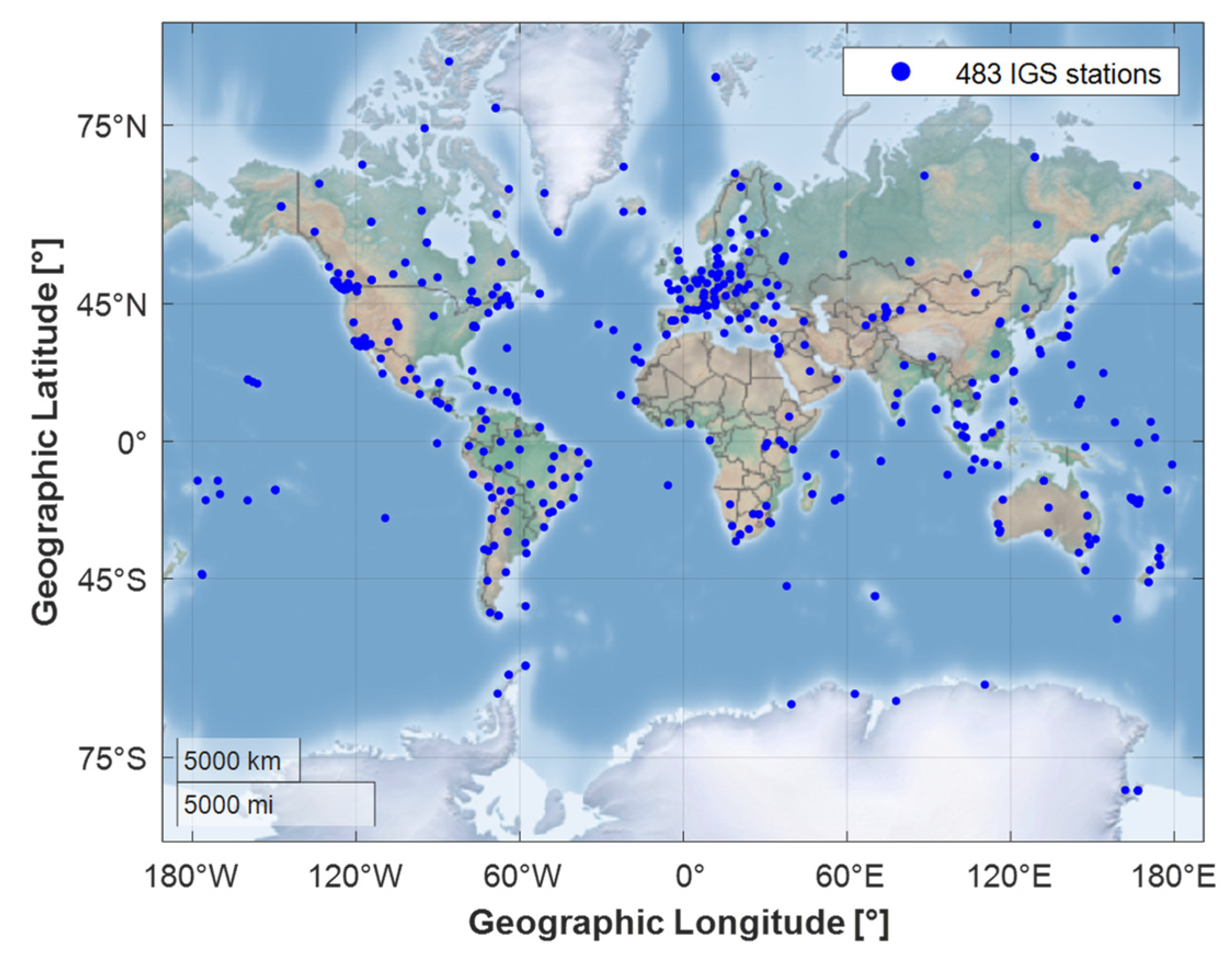
- IGS—International GNSS Service. Available online: https://igs.org/network/#station-map-list (accessed on 1 October 2021).
- Basu, S.; MacKenzie, E.; Sa, B. Ionospheric constraints on VHF/UHF communications links during solar maximum and minimum periods. Radio Sci. 1988, 23, 363–378. [Google Scholar] [CrossRef]
- Basu, S.; Groves, K.; Sultan, P. Specification and forecasting of scintillations in communication/navigation links: Current status and future plans. J. Atmos. Sol.-Terr. Phys. 2002, 64, 1745–1754. [Google Scholar] [CrossRef]
- Kintner, P.M.; Humphreys, T.; Hinks, J. GNSS and Ionospheric Scintillation, How to Survive the Next Solar Maximum; Trade Magazine Article; Cornell University: Ithaca, NY, USA; University of Texas at Austin: Austin, TX, USA, 2009. [Google Scholar]
- Tsai, L.-C.; Su, S.-Y.; Liu, C.-H. Global morphology of ionospheric F-layer scintillations using FS3/COSMIC GPS radio occultation data. GPS Solut. 2016, 21, 1037–1048. [Google Scholar] [CrossRef]


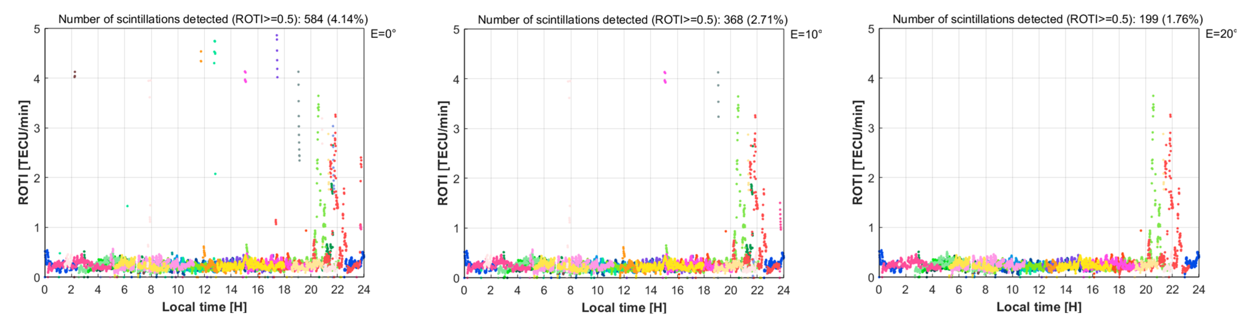
| Elevation Cut-Off | Number of Scintillations (ROTI ≥ 0.5) Detected | Percentage of Scintillations (ROTI ≥ 0.5) Detected |
|---|---|---|
| 0° | 584 | 4.14% |
| 10° | 368 | 2.71% |
| 20° | 199 | 1.76% |
| 30° | 197 | 2.25% |
| 40° | 165 | 2.59% |
| Time Span of Calculation (Minute) | Number of Scintillations (ROTI ≥ 0.5) Detected | Percentage of Scintillations (ROTI ≥ 0.5) Detected |
|---|---|---|
| 1 | 229 | 2.03% |
| 5 | 199 | 1.76% |
| 10 | 232 | 2.06% |
| 15 | 267 | 2.37% |
| 20 | 281 | 2.49% |
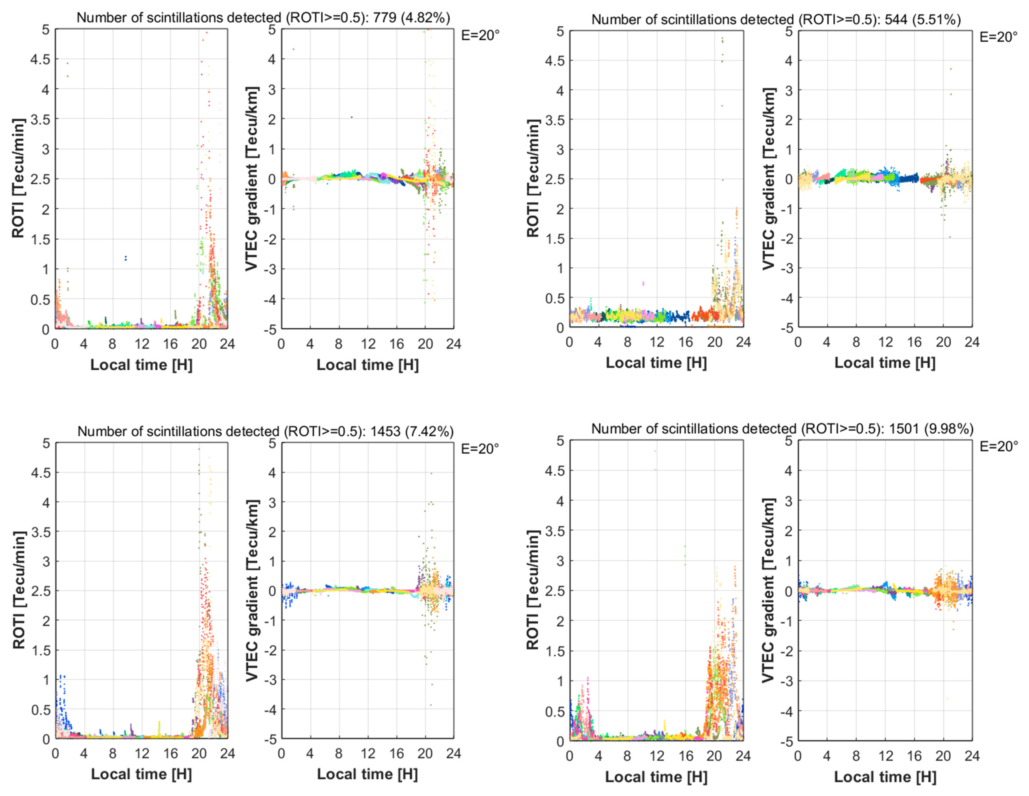
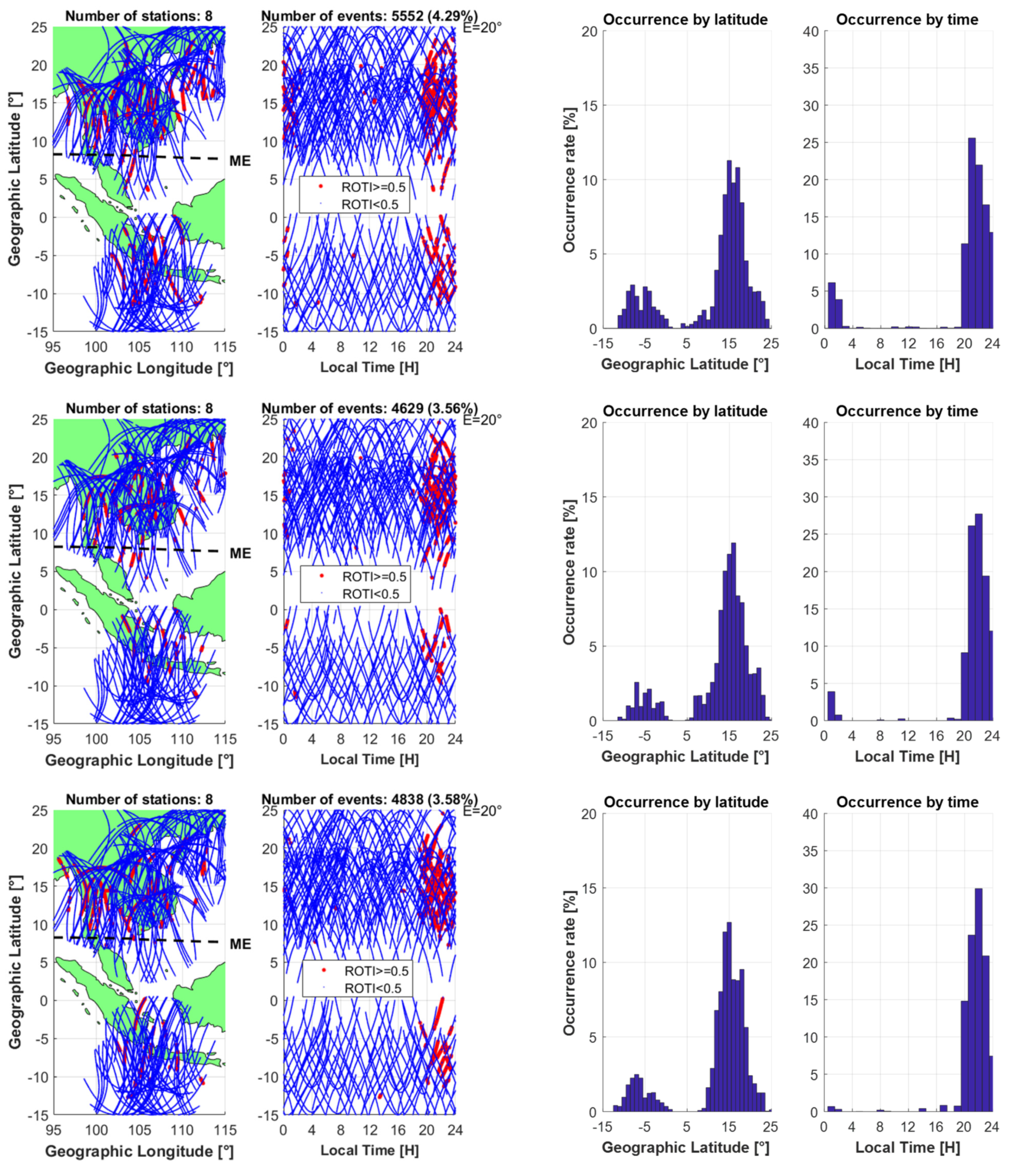
| Days of October | HANOI Station | HUE Station | Regional ROTI Maps | ||||||||
|---|---|---|---|---|---|---|---|---|---|---|---|
| S4 | ROTI | S4 | ROTI | ||||||||
| Num | % | Num | % | Num | % | Num | % | Num | % | Num of Stations | |
| 18 | 0 | 0.0 | 0 | 0.0 | 0 | 0.0 | 10 | 0.1 | 54 | 0.0 | 8 |
| 19 | 172 | 1.8 | 224 | 2.2 | 154 | 1.6 | 1039 | 7.5 | 5552 | 4.3 | 8 |
| 20 | 143 | 1.5 | 44 | 0.4 | 108 | 1.1 | 980 | 6.1 | 4629 | 3.6 | 8 |
| 21 | 0 | 0.0 | 0 | 0.0 | 11 | 0.1 | 44 | 0.3 | 1211 | 0.9 | 8 |
| 22 | 59 | 0.6 | 16 | 0.2 | 141 | 1.4 | 666 | 4.5 | 2729 | 2.3 | 8 |
| 23 | 1 | 0.0 | 0 | 0.0 | 7 | 0.1 | 140 | 0.8 | 337 | 0.3 | 8 |
| 24 | 63 | 0.6 | 201 | 1.8 | 154 | 1.6 | 533 | 3.5 | 4196 | 3.5 | 7 |
| 25 | 0 | 0.0 | no data | 0 | 0.0 | 18 | 0.1 | 209 | 0.2 | 7 | |
| 26 | 52 | 0.5 | 101 | 1.0 | 44 | 0.5 | 572 | 3.5 | 4838 | 3.6 | 8 |
| 27 | 2 | 0.0 | 1 | 0.0 | 44 | 0.4 | 163 | 0.9 | 968 | 0.7 | 8 |
| 28 | 98 | 1.0 | 11 | 0.1 | 229 | 2.3 | 1243 | 7.9 | 4221 | 3.2 | 8 |
| 29 | 35 | 0.4 | 15 | 0.2 | 45 | 0.5 | 251 | 1.5 | 1313 | 1.0 | 8 |
| 30 | 23 | 0.2 | 18 | 0.1 | 28 | 0.5 | 216 | 2.3 | 1406 | 1.2 | 8 |
| 31 | 0 | 0.0 | 0 | 0.0 | 217 | 2.2 | 1501 | 10.0 | 5434 | 4.5 | 8 |
| Days of March | HANOI Station | HUE Station | Regional ROTI Maps | ||||||||
|---|---|---|---|---|---|---|---|---|---|---|---|
| S4 | ROTI | S4 | ROTI | ||||||||
| Num | % | Num | % | Num | % | Num | % | Num | % | Num of Stations | |
| 15 | 0 | 0.0 | no data | 2 | 0.0 | 38 | 0.4 | 1383 | 1.0 | 8 | |
| 16 | 189 | 2.0 | 196 | 1.8 | 130 | 1.4 | 661 | 4.3 | 4785 | 3.0 | 9 |
| 17 | 0 | 0.0 | 4 | 0.0 | 0 | 0.0 | 2 | 0.0 | 318 | 0.2 | 9 |
| 18 | 0 | 0.0 | 3 | 0.0 | 0 | 0.0 | 13 | 0.1 | 225 | 0.1 | 9 |
| 19 | 233 | 2.5 | 285 | 3.0 | 82 | 0.9 | 36 | 0.3 | 1197 | 0.8 | 9 |
| 20 | 0 | 0.0 | 11 | 0.1 | 1 | 0.0 | 0 | 0.0 | 129 | 0.1 | 9 |
| 21 | 0 | 0.0 | 0 | 0.0 | 0 | 0.0 | 0 | 0.0 | 97 | 0.1 | 8 |
| 22 | 0 | 0.0 | 0 | 0.0 | 0 | 0.0 | 53 | 0.4 | 163 | 0.1 | 8 |
| 23 | 1 | 0.0 | 0 | 0.0 | 0 | 0.0 | 7 | 0.1 | 38 | 0.0 | 9 |
| 24 | 28 | 0.3 | 92 | 0.9 | 46 | 0.5 | 428 | 3.3 | 1784 | 1.3 | 9 |
| 25 | 10 | 0.1 | 33 | 0.3 | 35 | 0.4 | 110 | 0.7 | 617 | 0.4 | 9 |
| 26 | 174 | 1.9 | 71 | 0.9 | 173 | 1.8 | 799 | 5.5 | 4884 | 3.2 | 9 |
| 27 | 32 | 0.3 | 58 | 0.5 | 99 | 1.0 | 183 | 1.5 | 1468 | 1.2 | 8 |
| 28 | 24 | 0.3 | 20 | 0.2 | 27 | 0.3 | 167 | 1.3 | 1261 | 1.1 | 7 |
| Sector | Latitude Boundary [°] | Longitude Boundary [°] | Area Percentage [%] | Irregularity Percentages [%] | Irregularity Coefficients |
|---|---|---|---|---|---|
| South America | [−30:30] | [−100:−30] | 6.5 | 22.6 | 3.49 |
| Arctic | [60:90] | [−180:180] | 16.7 | 32.4 | 1.94 |
| West Africa | [−30:30] | [−30:20] | 4.6 | 8.2 | 1.77 |
| Southeast Asia | [−30:30] | [90:130] | 3.7 | 4.7 | 1.27 |
| South Asia | [−30:30] | [70:90] | 1.9 | 2.3 | 1.24 |
| Antarctic | [−90:−60] | [−180:180] | 16.7 | 18.3 | 1.10 |
| East Africa | [−30:30] | [20:70] | 4.6 | 4.1 | 0.89 |
| The Pacific | [−30:30] | [−180:−100] & [130:180] | 12.0 | 3.8 | 0.32 |
| Northern mid−latitudes | [30:60] | [−180:180] | 16.7 | 2.5 | 0.15 |
| Southern mid−latitudes | [−60:−30] | [−180:180] | 16.7 | 1.0 | 0.06 |
Publisher’s Note: MDPI stays neutral with regard to jurisdictional claims in published maps and institutional affiliations. |
© 2021 by the authors. Licensee MDPI, Basel, Switzerland. This article is an open access article distributed under the terms and conditions of the Creative Commons Attribution (CC BY) license (https://creativecommons.org/licenses/by/4.0/).
Share and Cite
Nguyen, C.T.; Oluwadare, S.T.; Le, N.T.; Alizadeh, M.; Wickert, J.; Schuh, H. Spatial and Temporal Distributions of Ionospheric Irregularities Derived from Regional and Global ROTI Maps. Remote Sens. 2022, 14, 10. https://doi.org/10.3390/rs14010010
Nguyen CT, Oluwadare ST, Le NT, Alizadeh M, Wickert J, Schuh H. Spatial and Temporal Distributions of Ionospheric Irregularities Derived from Regional and Global ROTI Maps. Remote Sensing. 2022; 14(1):10. https://doi.org/10.3390/rs14010010
Chicago/Turabian StyleNguyen, Chinh Thai, Seun Temitope Oluwadare, Nhung Thi Le, Mahdi Alizadeh, Jens Wickert, and Harald Schuh. 2022. "Spatial and Temporal Distributions of Ionospheric Irregularities Derived from Regional and Global ROTI Maps" Remote Sensing 14, no. 1: 10. https://doi.org/10.3390/rs14010010
APA StyleNguyen, C. T., Oluwadare, S. T., Le, N. T., Alizadeh, M., Wickert, J., & Schuh, H. (2022). Spatial and Temporal Distributions of Ionospheric Irregularities Derived from Regional and Global ROTI Maps. Remote Sensing, 14(1), 10. https://doi.org/10.3390/rs14010010