Article

A Lightweight Convolutional Neural Network Based on Channel Multi-Group Fusion for Remote Sensing Scene Classification

1
College of Communication and Electronic Engineering, Qiqihar University, Qiqihar 161000, China
2
College of Information and Communication Engineering, Dalian Nationalities University, Dalian 116000, China
*
Author to whom correspondence should be addressed.
Remote Sens. 2022, 14(1), 9; https://doi.org/10.3390/rs14010009
Submission received: 21 November 2021 / Revised: 17 December 2021 / Accepted: 20 December 2021 / Published: 21 December 2021
(This article belongs to the Special Issue Deep Reinforcement Learning in Remote Sensing Image Processing)

Abstract

:
With the development of remote sensing scene image classification, convolutional neural networks have become the most commonly used method in this field with their powerful feature extraction ability. In order to improve the classification performance of convolutional neural networks, many studies extract deeper features by increasing the depth and width of convolutional neural networks, which improves classification performance but also increases the complexity of the model. To solve this problem, a lightweight convolutional neural network based on channel multi-group fusion (LCNN-CMGF) is presented. For the proposed LCNN-CMGF method, a three-branch downsampling structure was designed to extract shallow features from remote sensing images. In the deep layer of the network, the channel multi-group fusion structure is used to extract the abstract semantic features of remote sensing scene images. The structure solves the problem of lack of information exchange between groups caused by group convolution through channel fusion of adjacent features. The four most commonly used remote sensing scene datasets, UCM21, RSSCN7, AID and NWPU45, were used to carry out a variety of experiments in this paper. The experimental results under the conditions of four datasets and multiple training ratios show that the proposed LCNN-CMGF method has more significant performance advantages than the compared advanced method.

1. Introduction

The goal of remote sensing scene image classification is to correctly classify the input remote sensing images. Due to the wide application of remote sensing image classification in natural disaster detection, land cover analysis, urban planning and national defense security [1,2,3,4], the classification of remote sensing scene images has attracted extensive attention. In order to improve the performance of remote sensing scene classification, many methods have been proposed. Among them, convolutional neural networks have become one of the most successful deep learning methods with their strong feature extraction ability. Convolutional neural networks are widely used in image classification [5] and target detection [6]. Many excellent neural networks have been designed for image classification. For example, Li et al. [7] proposed a deep feature fusion network for remote sensing scene classification. Zhao et al. [8] proposed a multi-topic framework combining local spectral features, global texture features and local structure features to fuse features. Wang et al. [9] used an attention mechanism to adaptively select the key parts of each image, and then fused the features to generate more representative features.
In recent years, designing a convolutional neural network to achieve the optimal trade-off between classification accuracy and running speed has become a research hotspot. SqueezeNet [10] designed a lightweight network by squeezing and extending modules to reduce parameter weight. In the SqueezeNet structure, three strategies are mainly used to reduce the parameters of the model. Firstly, partial 3 × 3 convolution is replaced by 1 × 1 convolution, then the number of input channels of 3 × 3 convolution kernel is reduced, and downsampling is carried out in the later part of the network to provide a larger features map for the convolution layer. The traditional convolution is decomposed in MobileNetV1 [11] to obtain the depthwise separable convolution. The depthwise separable convolution is divided into two independent processes: a lightweight depthwise convolution for spatial filtering and a 1 × 1 convolution for generating features, which separates spatial filtering from the feature generation mechanism. MobileNetV2 [12] added a linear bottleneck and inverted residuals structure on the basis of MobileNetV1, which further improves the performance of the network. SENet [13] proposed the SE module, which consists of extrusion and expansion. Firstly, extrusion is accomplished by global average pooling, which transforms the input two-dimensional feature channel into a real number with a global receptive field. Then, expansion is accomplished through the full connection layer, and a set of weighting parameters is obtained. Finally, channel-by-channel weighting is multiplied to complete the re-calibration of the original feature on the channel dimension. NASNet [14] used the enhanced learning and model search structure to learn a network unit in a small dataset, then stacked the learned units on a large dataset, which solves the problem that the previous neural network search structure cannot be applied to a large dataset. MobileNetV3 [15] added a SE module and used a neural structure search to search for network configuration and parameters. ResNet [16] solved performance degradation due to network depth using residual connectivity, and presents an efficient bottleneck structure with satisfactory results. Xception [17] replaced the convolution operation in the Inception module with depthwise separable convolution and achieves better performance. GoogleNet [18] used the Inception module to make the network deeper and wider. The Inception module consists of three convolution branches and one pooled branch, and finally four branches were fused through channels.
Grouped convolution was first used in AlexNet [19]. Due to the limitations of hardware conditions at that time, it was used in AlexNet to slice the network, which made it run parallel with two GPUs and achieved good performance. The validity of grouping convolution is well demonstrated in ResNeXt [20]. ResNeXt highly modularizes the network structure, building a network architecture by repeating stacked modules. The module is composed of several bottleneck structures, which improves the accuracy of the model without increasing the number of parameters. Traditional channel grouping uses a single grouping form (for example, the number of channels of input features is C , g is the number of groups, and the number of channels in each group is C / g ). Using a single channel group is not conducive to feature extraction; to solve this problem, we proposed a channel multi-group convolution structure. The structure classifies the input features into two types of grouping, the number of channels for each set of features in the first type is C / g , and the number of channels for each set of features in the other type is 2 C / g . The channel multi-group structure increases the diversity of features while decreasing the parameters further. To reduce the loss of feature information during the grouping convolution process, residual connection is added to the channel multi-group structure, which can effectively avoid the disappearance of gradient due to network deepening. In order to solve the problem of network performance degradation caused by lack of information interaction between individual groups during group convolution, channel fusion of adjacent features is carried out to increase information interaction and improve network feature representation ability.
The main contributions of this study are as follows.
(1)
In the shallow layer of the network, a shallow feature extraction module is constructed. The module is composed of three branches. Branch 1 uses two consecutive 3 × 3 convolution for downsampling and feature extraction, branch 2 utilizes max-pooling and 3 × 3 convolution for downsampling and feature extraction. Branch 3 is a shortcut branch. The fused features of branch 1 and branch 2 are shortcut with branch 3. The module can fully extract the shallow feature information, so as to accurately distinguish the target scene.
(2)
In the deep layer of the network, a channel multi-group fusion module is constructed for the extraction of deep features, which divided the input features into features with channel number of C / g and channel number of 2 C / g , increasing the diversity of features.
(3)
To solve the problem of lack of information interaction for features between groups due to group convolution, in the channel multi-group module, the channel fusion of adjacent features is utilized to increase the information exchange, which significantly improves the performance of the network.
(4)
A lightweight convolutional neural network is constructed based on channel multi-group fusion (LCNN-CMGF) for remote sensing scene image classification, which includes shallow feature extraction module and channel multi-group fusion module. Moreover, a variety of experiments are carried out under the conditions of four datasets of UCM21, RSSCN7, AID and NWPU45, and the experimental results prove the proposed LCNN-CMGF method achieves the trade-off between model classification accuracy and running speed.
The rest of this paper is as follows. In Section 2, the overall structure, shallow feature extraction module and channel multi-group module of the proposed LCNN-CMGF method are described in detail. Section 3 provides the experimental results and analysis. In Section 4, several visualization methods are adopted to evaluate the proposed LCNN-GMGF method. The conclusion of this paper is given in Section 5.

2. Methods

2.1. The Overall Structure of Proposed LCNN-CMGF Methods

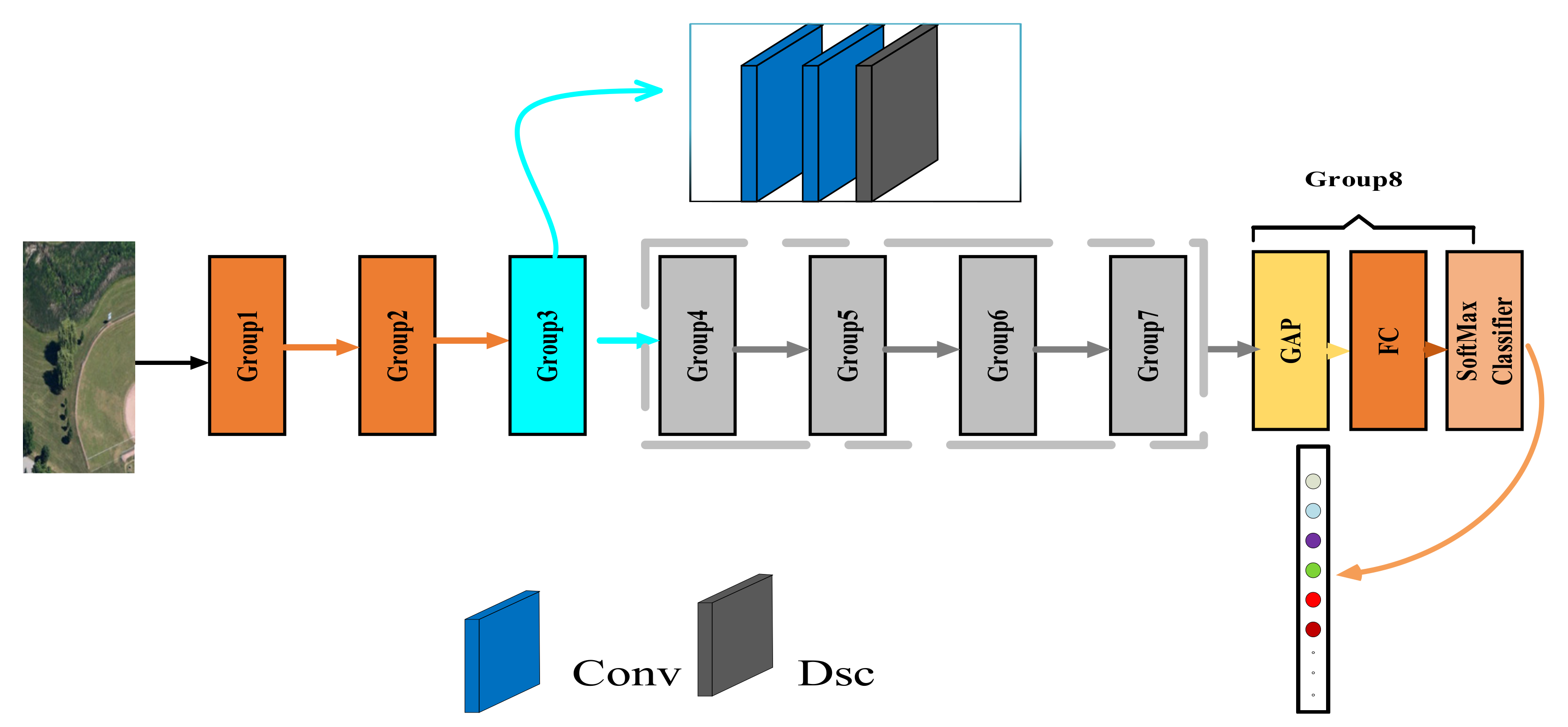
As shown in Figure 1, the proposed network structure is divided into eight groups, the first three being used to extract shallow information from remote sensing images. Groups 1 and 2 adopt a proposed shallow downsampling structure, which is introduced in Section 2.2 in detail. Group 3 uses a hybrid convolution method combining standard convolution and depthwise separable convolution for feature extraction. Depthwise separable convolution has a significant reduction in the number of parameters compared with standard convolution. Assuming that the input feature size is H × W × C 1 , the convolution kernel size is H 1 × W 1 × C 1 and the output feature size is H × W × C 2 , the parameter quantity of standard convolution is:
p a r a m s c o n v = H 1 × W 1 × C 1 × C 2
The parameter quantities of depthwise separable convolution is:
p a r a m s d s c = H 1 × W 1 × C 1 + C 1 × C 2
The ratio p a r a m s d s c / p a r a m s c o n v of depthwise separable convolution to standard convolution is:
p a r a m s d s c p a r a m s c o n v = H 1 × W 1 × C 1 + C 1 × C 2 H 1 × W 1 × C 1 × C 2 = 1 C 2 + 1 H 1 × W 2
According to Equation (3), when the convolution kernel size H 1 × W 2 is equal to 3 × 3, due to C 2 H 1 × H 2 , the parameter quantity of standard convolution is approximately 9 times that of depthwise separable convolution, and when the convolution kernel size H 1 × W 2 is equal to 5 × 5, the parameter of standard convolution is approximately 25 times that of depthwise separable convolution. With the increase in convolution kernel size, the parameter will be further reduced. However, depthwise separable convolution can inevitably lead to the loss of some feature information while significantly reducing the amount of parameters, and then make the learning ability of the network decline. Therefore, we propose to use the hybrid convolution of standard convolution and depthwise separable convolution for feature extraction, which not only reduces the weight parameters, but also improves the learning ability of the network. From group 4 to group 7, channel multi-group fusion structure is used to further extract deep feature information. Channel multi-group fusion structure can generate a large number of features with a few parameters to increase the feature diversity. Assuming that the input feature size is H × W × C 1 , the convolution kernel size is H 1 × W 1 × C 1 and the output feature size is H × W × C 2 , the parameter quantity of standard convolution is
p a r a m s c o n v = H 1 × W 1 × C 1 × C 2
Divide the input features into t groups along the channel dimension, then the feature size of each group is H × W × C 1 t , the corresponding convolution kernel size is H 1 × W 1 × C 1 t , and the output feature size of each group is H × W × C 2 t . Connect the obtained t group features along the channel dimension to obtain that the final output feature size is H × W × C 2 . The parameter quantity of the whole process is
p a r a m s g c o n v = H 1 × W 1 × C 1 t × C 2 t × t = H 1 × W 1 × C 1 × C 2 × 1 t
As shown in Equations (4) and (5), the parameter quantity of group convolution is 1 / t of the standard convolution parameter quantity, that is, under the condition of the same parameter quantity, the number of features obtained by group convolution is t times of the standard convolution, which increases the feature diversity and effectively improves the classification accuracy. The details are described in Section 2.3. Group 8 consists of a global average pooling layer (GAP), a fully connected layer (FC), and a softmax classifier to convert the convolutionally extracted feature information into probabilities for each scenario. Because features extracted by convolution contain spatial information, which is destroyed if features derived by convolution are directly mapped to the feature vector through a fully connected layer, and global average pooling does not. Assuming that the output of the last convolution layer is O = [ o 1 ; o 2 ; ; o i ; o N ] N × H × W × C , [ ; ; ; ] represents cascading operations along the batch dimension, and represents the set of real numbers. In addition, N , H , W , C represent the number of samples per training, the height of the feature, the width of the feature, and the number of channels, respectively. Suppose the result of global average pooling is P = [ p 1 ; p 2 ; ; p i ; p N ] N × 1 × 1 × C , then the processing process of any P = [ p 1 ; p 2 ; ; p i ; p N ] N × 1 × 1 × C with the global average pooling layer can be represented as
p i = 1 H × W h = 1 H w = 1 W o i
As shown in Equation (6), global average pooling more intuitively maps the features of the last layer convolution output to each class. Additionally, the global average pooling layer does not require weight parameters, which can avoid overfitting phenomena during training the model. Finally, a softmax classifier is used to output probability values for each scenario.

2.2. The Three-Branch Shallow Downsampling Structure

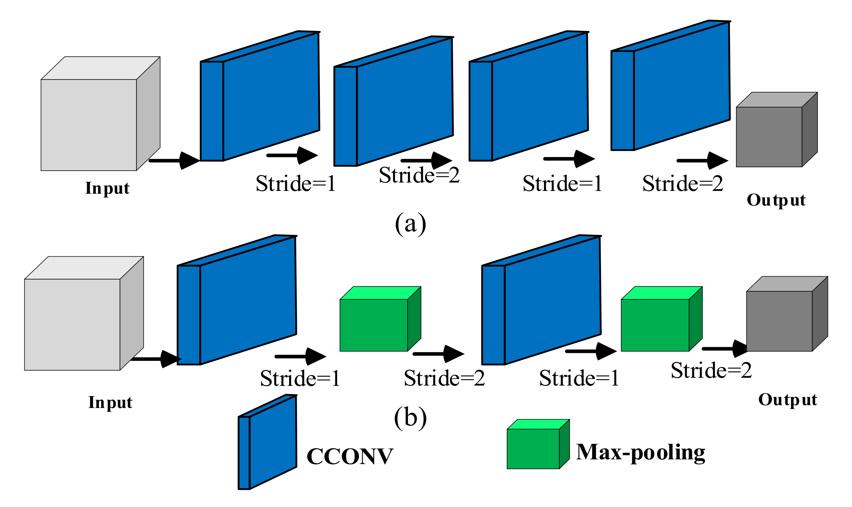
Max-pooling downsampling is a nonlinear downsampling method. For small convolutional neural networks, better nonlinearity can be obtained by using maximum pool downsampling. On the contrary, for deep neural networks, multi-layer superimposed convolutional downsampling can learn better nonlinearity than max-pooling according to the training set, as shown in Figure 2. Figure 2a,b represents convolution downsampling and max-pooling downsampling, respectively. The convolution downsampling in Figure 2a first uses the 3 × 3 convolution with step size of 1 for feature extraction of the input data, and then uses the 3 × 3 convolution with step size of 2 for downsampling. In the max-pooling downsampling in Figure 2b, the input feature is extracted by 3 × 3 convolution with step size of 1, and then the max-pooling downsampling with step size of 2 is adopted. Combining max-pooling downsampling and convolutional downsampling, we propose a three-branch downsampling structure as shown in Figure 3 for feature extraction, and use the input features to compensate the downsampling features, which can not only extract strong semantic features, but also retain shallow information.
In groups 1 and 2 of the network, we use the structure shown in Figure 3 to extract shallow features. The structure is divided into three branches. The first branch uses 3 × 3 convolution with step size of 2 to obtain f d o w n , and then uses 3 × 3 convolution with step size of 1 to extract the shallow features of the image to obtain f 1 ( x ) . That is
f d o w n ( x ) = δ ( B N ( F K s = 2 ) )
f 1 ( x ) = δ ( B N ( f d o w n ( x ) K s = 1 ) )
In Equations (7) and (8), δ represents the activation function R u l e , B N represents batch standardization, F represents the input characteristics, K s represents the 3 × 3 convolution kernel with step size s , and represents the convolution operation.
The second branch uses the max-pooling with step size of 2 to downsample the input features to obtain f m i j . The most responsive part of the max-pooling selection features enters the next layer, which reduces the redundant information in the network and makes the network easier to be optimized. The max-pooling downsampling can also reduce the estimated mean shift caused by the parameter error of the convolution layer, keep more texture information. Then, the shallow features f 2 ( x ) are extracted by 3 × 3 convolution with step size of 1. That is
f m i j = max ( s , t ) R i j x m s t
f 2 ( x ) = δ ( B N ( f mij ( x ) K s = 1 ) )
In Equation (9), f m i j represents the max-pooling output value in rectangular area R i j related to the m-th feature, and x m s t represents the element at the ( s , t ) position in rectangular area R i j .
The fused feature f ( x ) is obtained by fusing the features from Branch 1 and Branch 2. To reduce the loss of feature information caused by the first two branches, a residual branch is constructed to compensate for the loss of information. The fused feature f ( x ) and the third branch are fused to generate the final output feature y ( x ) . That is
y ( x ) = g ( x ) + f ( x )
The g ( x ) in Equation (11) is a residual connection implemented by 1 × 1 convolution.

2.3. Channel Multi-Group Fusion Structure

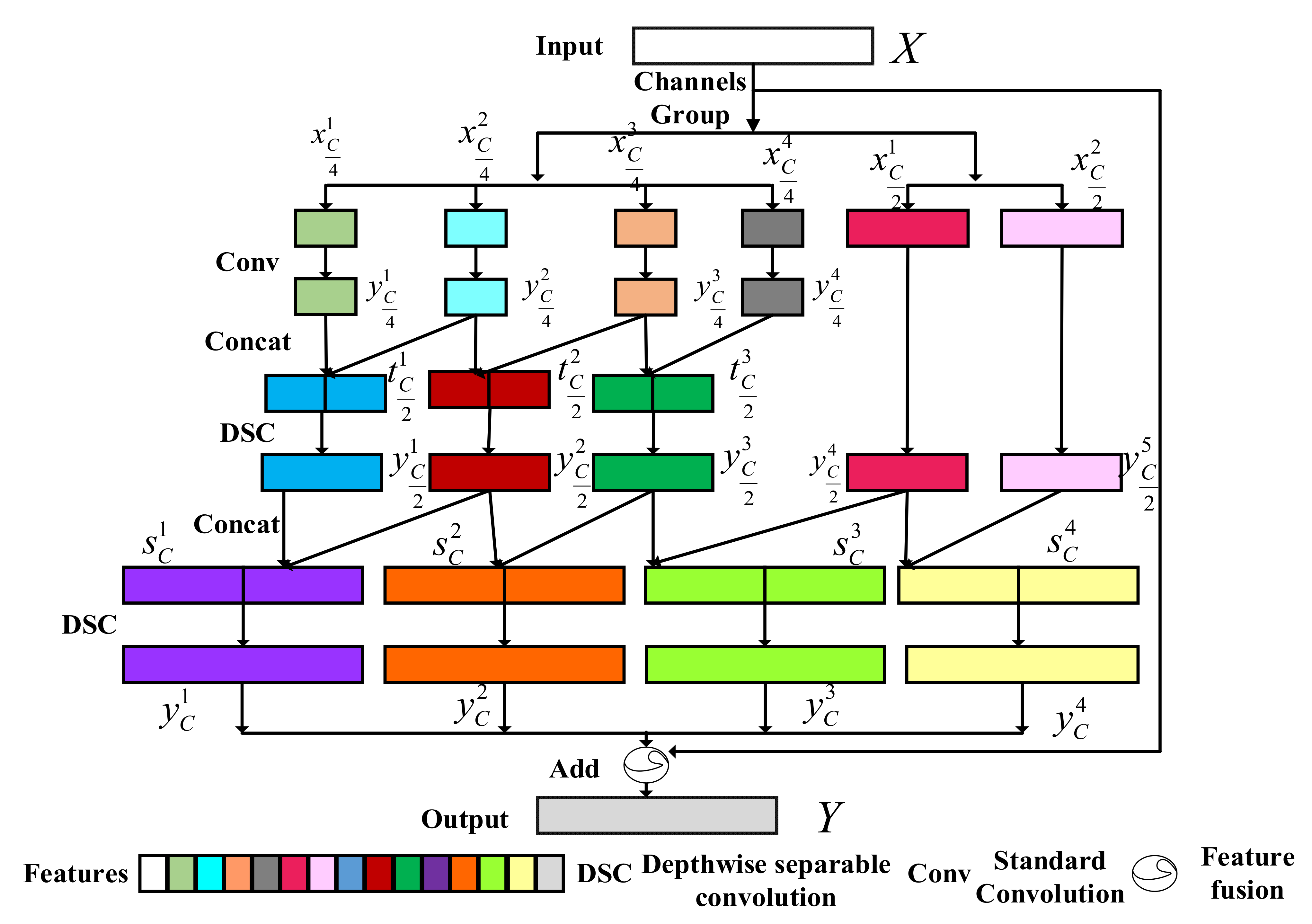
The proposed channel multi-group fusion structure is shown in Figure 4. It divides the input features with the number of channels C into two parts, one part is composed of 4 features with the number of channels C 4 , and the other part is composed of 2 features with the number of channels C 2 . First, the convolution operations are performed for features with the number of channels C 4 , the adjacent two convolution results are channel concatenated, the number of feature channels after concatenate is C 2 . Then, the convolution operations are performed on features with the number of channels C 2 , the adjacent two features convolution results are channel concatenated, the number of channels of each feature after fusion was C . The convolution operations are performed on features with the number of channels C , and the convolution results are fused to obtain the output features. This process can be described as follows.
Suppose that the input feature is X = [ x 1 , x 2 , , x C ] W × H × C , x C 4 i W × H × C 4 represents the i-th feature with the number of channels C 4 , and x C 2 i W × H × C 2 represents the i-th feature with the number of channels C 2 . After channel grouping, the input features can be represented as x C 4 1 = [ x 1 , , x C 4 ] , x C 4 2 = [ x C 4 , , x C 2 ] , x C 4 3 = [ x C 2 , , x 3 C 4 ] , x C 4 4 = [ x 3 C 4 , , x C ] , x C 2 1 = [ x 1 , , x C 2 ] , x C 2 2 = [ x C 2 , , x C ] . The convolution operation is performed first for the features x C 4 1 , x C 4 2 , x C 4 3 , and x C 4 4 , where the number of channels is C 4 , and after convolution the results are y C 4 1 W × H × C 4 , y C 4 2 W × H × C 4 , y C 4 3 W × H × C 4 , and y C 4 4 W × H × C 4 , respectively. Here, y C 4 i can be represented as
y C 4 i = f c o n v ( x C 4 i , W ) = Re L U ( B N ( W x C 4 i ) )                   i = 1 , 2 , 3 , 4
y C 4 i represents the convolution result of the feature x C 4 i , and y C 4 i = [ y C 4 i ( 1 ) , y C 4 i ( 2 ) , , y C 4 i ( m ) , , y C 4 i ( C 4 ) ] . y C 4 i ( m ) represents the m-th channel of the i-th feature with the number of channels C 4 , f c o n v ( ) represents the convolution operation, W represents the convolution weight, Re L U represents the activation function, and B N represents batch normalization.
The use of grouping convolution can reduce the requirement of computing power, but it will also lead to the lack of information interaction between group features, which makes the extracted features incomplete. The information interaction is enhanced through channel concatenate of two adjacent features ( y C 4 1 , y C 4 2 ) , ( y C 4 2 , y C 4 3 ) and ( y C 4 3 , y C 4 4 ) . The number of feature channels after channel concatenate is C 2 , and t C 2 i W × H × C 2 represents the i-th feature after channel concatenate, the channel concatenate operation of feature ς and feature ϖ is represented by [ ς , ϖ ] , where t C 2 i is calculated as
t C 2 1 = m = 1 C 4 n = 1 C 4 ( [ y C 4 1 ( m ) , y C 4 2 ( n ) ] )
t C 2 2 = m = 1 C 4 n = 1 C 4 ( [ y C 4 2 ( m ) , y C 4 3 ( n ) ] )
t C 2 3 = m = 1 C 4 n = 1 C 4 ( [ y C 4 3 ( m ) , y C 4 4 ( n ) ] )
The features x C 2 1 , x C 2 2 , t C 2 1 , t C 2 2 , t C 2 3 with the number of channel C 2 are processed by depthwise separable convolution and the results after convolution are y C 2 1 W × H × C 2 , y C 2 2 W × H × C 2 , y C 2 3 W × H × C 2 , y C 2 4 W × H × C 2 , y C 2 5 W × H × C 2 respectively. y C 2 i is calculated as
y C 2 i = f d s c ( x C 2 i , W ) = Re L U ( B N ( W x C 2 i ) )           i = 1 , 2
y C 2 i = f d s c ( t C 2 j , W ) = Re L U ( B N ( W t C 2 j ) )       i = 3 , 4 , 5 ,       j = 1 , 2 , 3
where y C 2 i represents the convolution result of the features x C 2 i and t C 2 i , and y C 2 i = [ y C 2 i ( 1 ) , y C 2 i ( 2 ) , , y C 2 i ( m ) , , y C 2 i ( C 2 ) ] , y C 2 i ( m ) represents the m-th channel of the i-th feature with the number of channels C 2 , and f d s c ( ) represents the depthwise separable convolution operation. Then, the adjacent features ( y C 2 1 , y C 2 2 ) , ( y C 2 2 , y C 2 3 ) , ( y C 2 3 , y C 2 4 ) and ( y C 2 4 , y C 2 5 ) are concatenated in the channel dimension. The number of feature channels after concatenate is C , and s C i W × H × C represents the i-th feature with the number of channels after concatenate C . The calculation process of s C i is
s C 1 = m = 1 C 2 n = 1 C 2 ( [ y C 2 1 ( m ) , y C 2 2 ( n ) ] )
s C 2 = m = 1 C 2 n = 1 C 2 ( [ y C 2 2 ( m ) , y C 2 3 ( n ) ] )
s C 3 = m = 1 C 2 n = 1 C 2 ( [ y C 2 3 ( m ) , y C 2 4 ( n ) ] )
s C 4 = m = 1 C 2 n = 1 C 2 ( [ y C 2 4 ( m ) , y C 2 5 ( n ) ] )
The features s C 1 , s C 2 , s C 3 and s C 4 with the number of channels C are processed by depthwise separable convolution, respectively. The convolution results are y C 1 , y C 2 , y C 3 and y C 4 . The calculation process of y C i is
y C i = f d s c ( s C i , W ) = Re L U ( B N ( W s C i ) )           i = 1 , 2 , 3 , 4
Next, the features y C 1 , y C 2 , y C 3 , y C 4 are fused and the fusion results and input feature X are shortcut to obtain the final output result Y W × H × C , where denotes feature fusion.
Y = y C 1 y C 2 y C 3 y C 4 X

3. Experiment

In this section, the proposed LCNN-CMGF method is evaluated from multiple perspectives using different indicators. The four most commonly used remote sensing scene datasets, UCM21, RSSCN7, AID and NWPU45, are used to carry out a variety of experiments in this paper. The experimental results under the conditions of four datasets and multiple training ratios show that the proposed LCNN-CMGF method has more significant performance advantages than the compared advanced method.

3.1. Dataset Settings

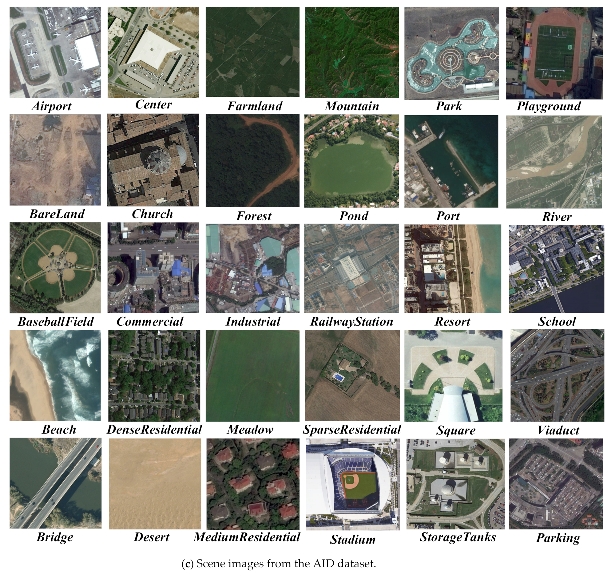
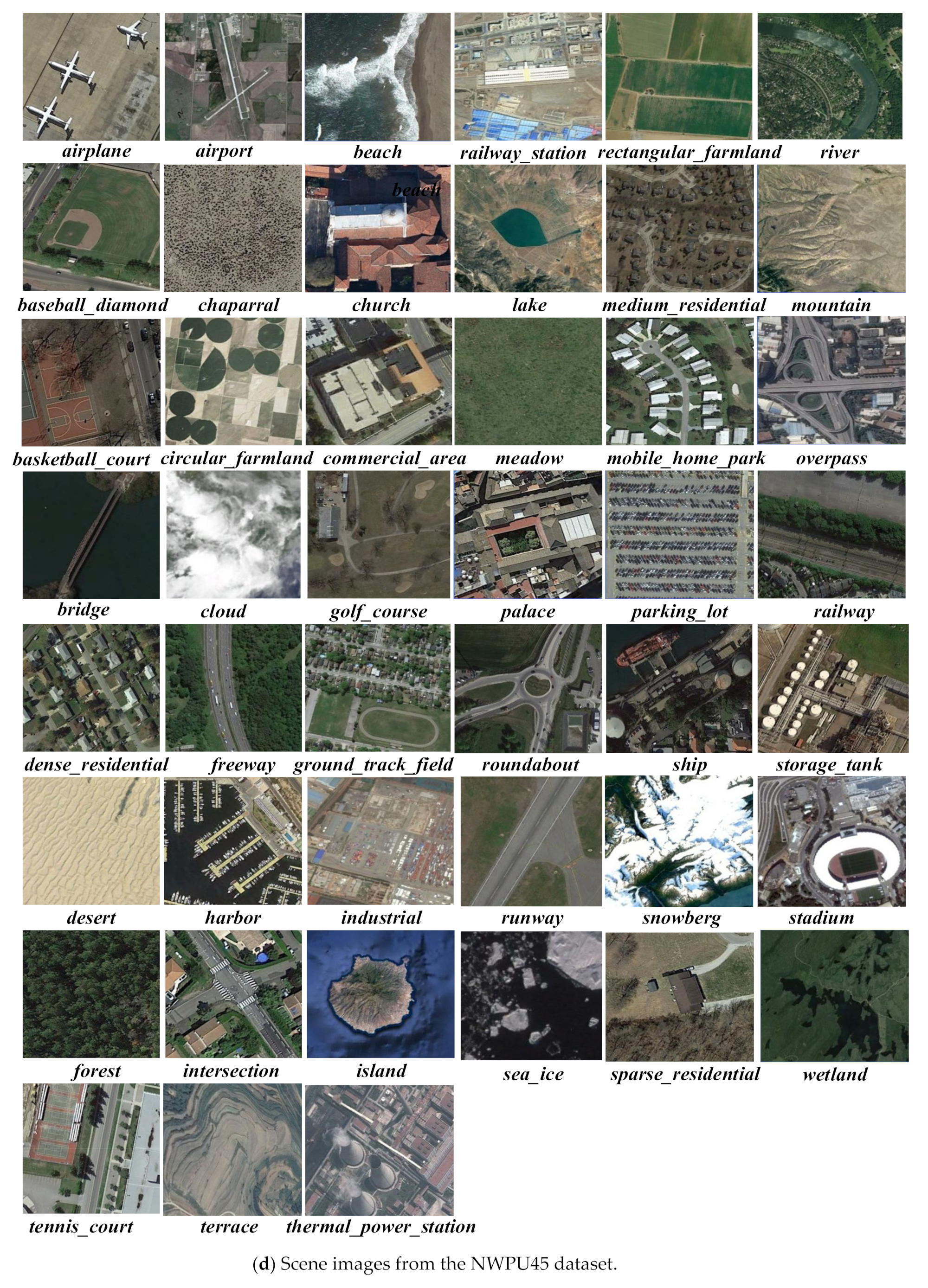
To verify the performance of the proposed LCNN-CMGF method, a series of experiments were performed on four datasets, i.e., UCM21 [21], RSSCN7 [22], AID [23], NWPU45 [24]. In addition to the complex spatial structure, remote sensing scene images also have high intra-class differences and similarities between classes, which make these four datasets very challenging. Details of the four datasets are shown in Table 1, including the number of images per class, the number of scene categories, the total number of images, the spatial resolution of images, and the image size. In addition, we select a scene image from each scene category of the four datasets for display, as shown in Figure 5. Due to the inconsistent size of the image, in order to avoid memory overflow in the training process, the bilinear interpolation method is used to adjust the size of the training image to 256 × 256.

3.2. Setting of the Experiments

When dividing the dataset, a stratified sampling method is adopted. The stratified sampling can effectively avoid the risk of sampling deviation. In stratified sampling, a random seed is set to ensure that the same images are chosen in each experiment. In addition, in order to improve the reliability of the experimental results, the average value of 10 experimental results is taken as the final result. According to previous work on remote sensing scene image classification, the datasets are divided as follows: the UCM21 [21] dataset is divided into training:test = 8:2, that is, 1680 scene images are used for training, and the remaining 420 scene images are used for testing; the RSSCN7 [22] dataset is divided into training:test = 5:5, that is, 1400 scene images are used for training, and the remaining 1400 scene images are used for testing; the AID30 [23] dataset is divided into training:test = 2:8 and training:test = 5:5, respectively. When training:test = 2:8, 2000 scene images for training and 8000 scene images for testing; When training:test = 5:5, 5000 scene images for training and 5000 scene images for testing; and the NWPU45 [24] dataset is divided into training:test = 1:9 and training:test = 2:8, respectively. When training:test = 1:9, 3150 scene images for training and 28,350 scene images for testing; When training:test = 2:8, 6300 scene images for training and 25,200 scene images for testing. As shown in Table 2, the input and output sizes of each group of features from group 1 to group 8 in the LCNN-CMGF method are listed. Table 3 shows the experimental environment and parameter setting.

3.3. Experimental Result

To verify the performance of the proposed method, evaluation indexes such as overall accuracy (OA), kappa coefficient (kappa), confusion matrix, and weighting parameters were used for experimental comparison.

3.3.1. Experimental Results on the UCM21 Dataset

The methods with good classification performance on the UCM21 dataset from 2019 to 2020 are selected for comparison with the proposed LCNN-CMGF method. The experimental results are shown in Table 4. Under the condition that the training proportion of the UCM21 dataset was 80%, the classification accuracy of the proposed LCNN-CMGF method reaches 99.52%, which exceeds all the comparison methods. The proposed LCNN-CMGF method is 0.6% higher than the Lie group (LiG) with sigmoid kernel [25], 0.55% higher than the Contourlet CNN method [26], and 3.19% higher than the MobileNet method [27]. Table 5 lists the kappa coefficient of the proposed LCNN-CMGF method and the comparison methods. The kappa coefficient of the proposed method is 99.50%, 6.13% higher than EfficientNet [28], and 2.58% higher than Fine tune Mobilenet V2 [29], which proves the effectiveness of our method.
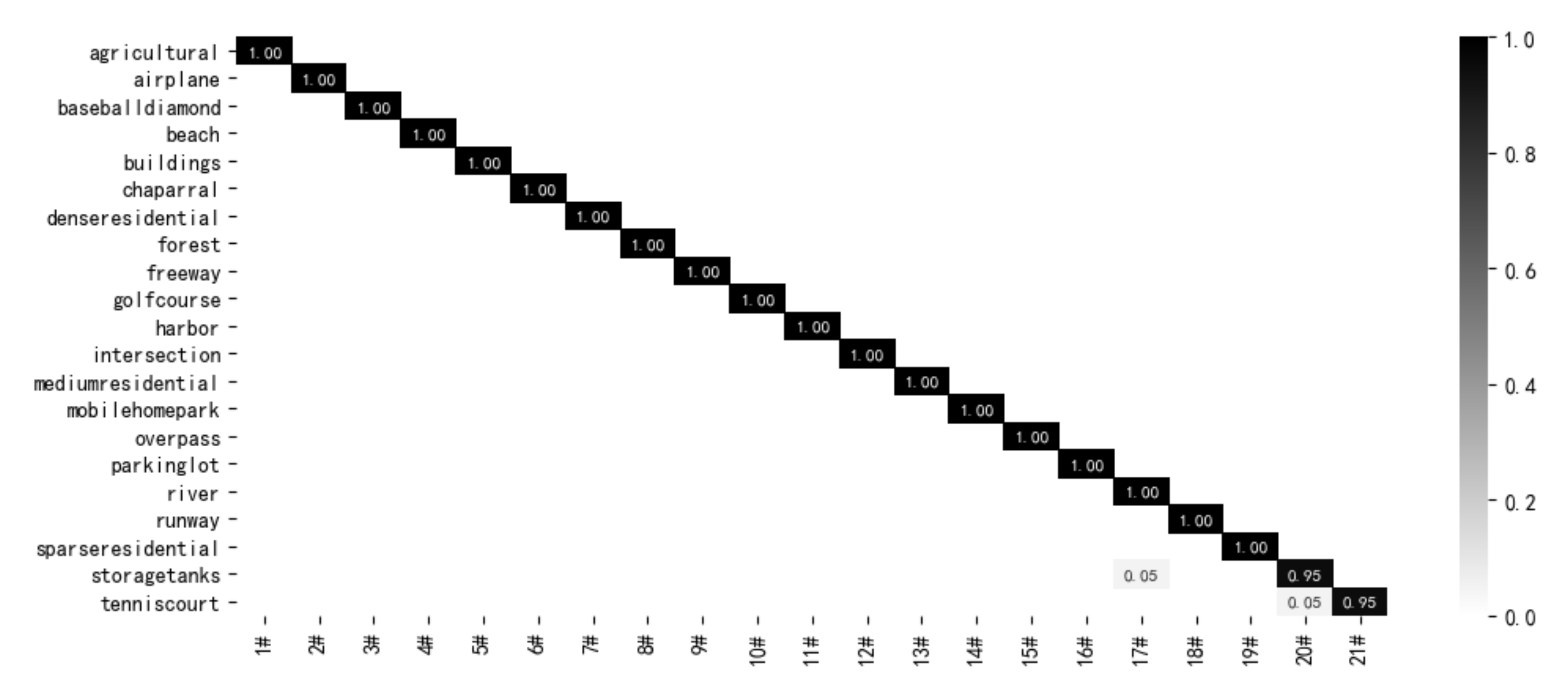
As shown in Figure 6, in the UCM21 dataset, except that the classification accuracy of two scenes of ‘storagetanks’ and ‘tenniscourt’ is 95%, the classification accuracy of other scenes is 100%. It is proved that this method has good performance on the UCM21 dataset.

3.3.2. Experimental Results on the RSSCN7 Dataset

The comparison of experimental results of the proposed methods and some state-of-the-art methods proposed in the last two years on RSSCN7 datasets are shown in Table 6. The OA of our proposed method is 97.50%, which is 0.85%, 3.9% and 1.52% higher than that of VGG-16-CapsNet [30], WSPM-CRC [31] and the Positional Context Aggregation method [32], respectively. It is proved that our method has better feature representation ability.
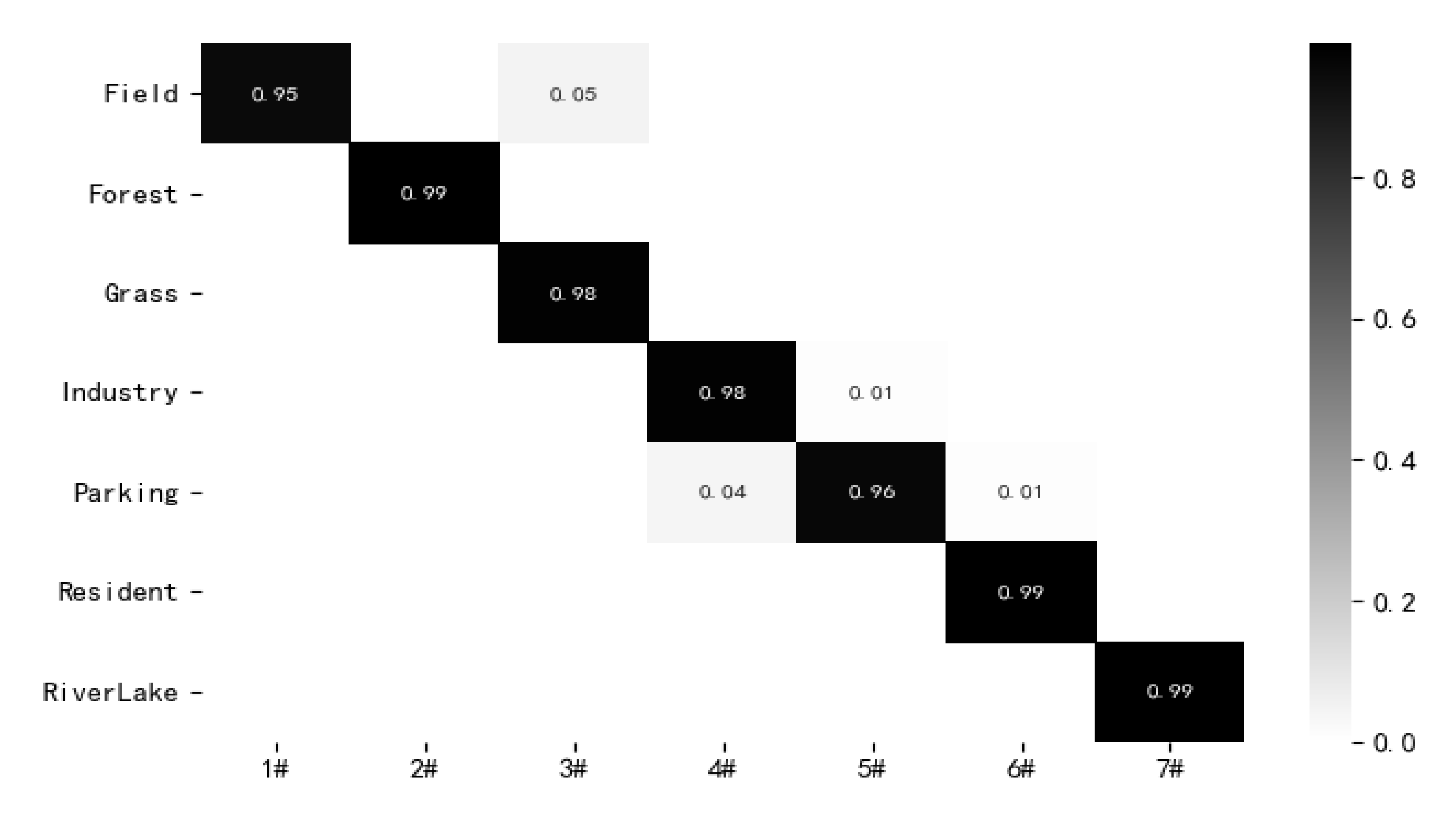
The confusion matrix of the proposed LCNN-CMGF method on the RSSCN7 dataset is shown in Figure 7. The proposed method has good classification accuracy on this dataset. The classification accuracy of all scenarios can reach more than 95%, and the classification accuracy of three scenarios, ‘Forest’, ‘RiverLake’, and ‘Resident’, can reach 99%. The classification accuracy of ‘Field’ scenes is the lowest 95%, and some of them are incorrectly classified into ‘Grass’ scenes, which is due to the strong class similarity between ‘Grass’ and ‘Field’ scenes.

3.3.3. Experimental Results on the AID Dataset

Some excellent CNN-based methods on the AID dataset from 2018 to 2020 are selected for comparison with the proposed method. The experimental results are shown in Table 7. Under the condition that the training proportion of the AID dataset was 20%, the classification accuracy of the proposed LCNN-CMGF method is 93.63%, which is 1.57% higher than that of LCNN-BFF [33], 2.07% higher than that of DDRL-AM Method [34], 2.53% higher than that of Skip-Connected CNN [35], and 1.43% higher than that of GBNet + Global Feature [36]. Under the condition that the training proportion of the AID dataset was 50%, the OA of the proposed method is reaching 97.54%, which is 2.09% higher than that of Feature Aggregation CNN [37], 2.28% higher than that of Aggregated Deep Fisher Feature [38], 0.79% higher than that of HABFNet [39], 2.15% higher than that of EfficientNetB3-Attn-2 [40], and 1.56% higher than that of VGG_VD16 with SAFF Method [41]. The experimental results show that the proposed method is very effective. For remote sensing scene images with rich image variation, high similarity between classes and strong intra-class differences, the proposed method can capture more representative features. As shown in Table 8, the Kappa coefficient of this method is 97.45% when the training proportion is 50%, which is 1.95% higher than that of Semi-Supervised Representation Learning [42], 1.33% higher than that of Variable-Weighted Multi-Fusion [43], 3.49% higher than that of TSDFF [44], and 3.19% higher than that of Discriminative+AlexNet [45]. The Kappa coefficient results demonstrate that the predicted and actual results of the proposed method are more consistent.
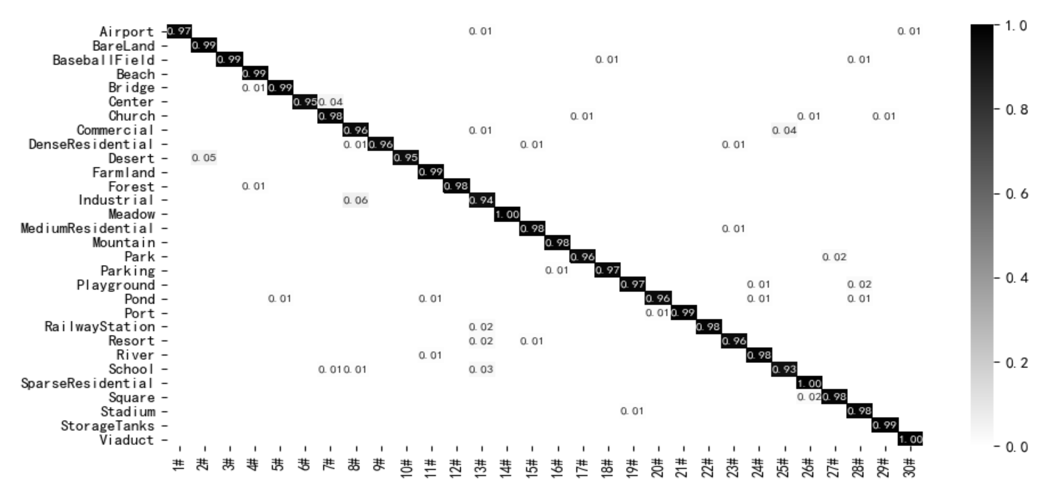
The confusion matrix of the LCNN-CMGF method on the 50/50 AID dataset is shown in Figure 8. The classification accuracy of all scenes has reached more than 90%, among which the classification accuracy of ‘Meadow’, ‘Viaduct’ and ‘Sparse Residential’ has reached 100%. In the training proportion of 50%, the classification accuracy of ‘School’ scenes is the lowest, which is 93%. Some school scenes are incorrectly classified into three scenes: ‘Industrial’, ‘Church’ and ‘Commercial’. The reason is that there are similar buildings among the four scenes of ‘School’, ‘Industrial’, ‘Church’ and ‘Commercial’. The high inter-class similarity leads to the low classification accuracy of the ‘School’ scene. For all that, the proposed method still achieved better classification performance compared with the previously proposed advanced method.

3.3.4. Experimental Results on the NWPU45 Dataset

Similar to the AID dataset, some excellent neural networks on the NWPU45 dataset from 2018 to 2020 are selected for experimental comparison. The experimental results are shown in Table 9. When training:test = 1:9, the OA of the proposed method reached 92.53%, which is 6% higher than that of the LCNN-BFF method [33], 8.15% higher than that of VGG_VD16 with the SAFF method [41], 3.31% higher than that of Discriminative + VGG16 [45], 11.19% higher than that of VGG19 [46] and 0.97% higher than that of MSDFF [50], respectively. When training:test = 2:8, the OA of the proposed method is 6.6% and 2.45% higher than that of Contourlet CNN [26] and the LCNN-BFF method [33], respectively. Meanwhile, the OA of the proposed method is 8.2% higher than that of Skip-Connected CNN [35] and 3.31% higher than that of Discriminative + VGG16 [45]. This indicates that the proposed method performs better on both training ratios on NWPU45 datasets. Under the condition that the training proportion is 20% in the NWPU45 dataset, the kappa coefficient contrast results for the proposed LCNN-CMGF method and the contrast method are shown in Table 10. The Kappa value of this method is the highest among all comparison methods, reaching 94.04%. It is 1.12%, 5.69% and 10.72% higher than that of LiG with sigmoid kernel [25], Contourlet CNN [26] and MobileNet [27], respectively.
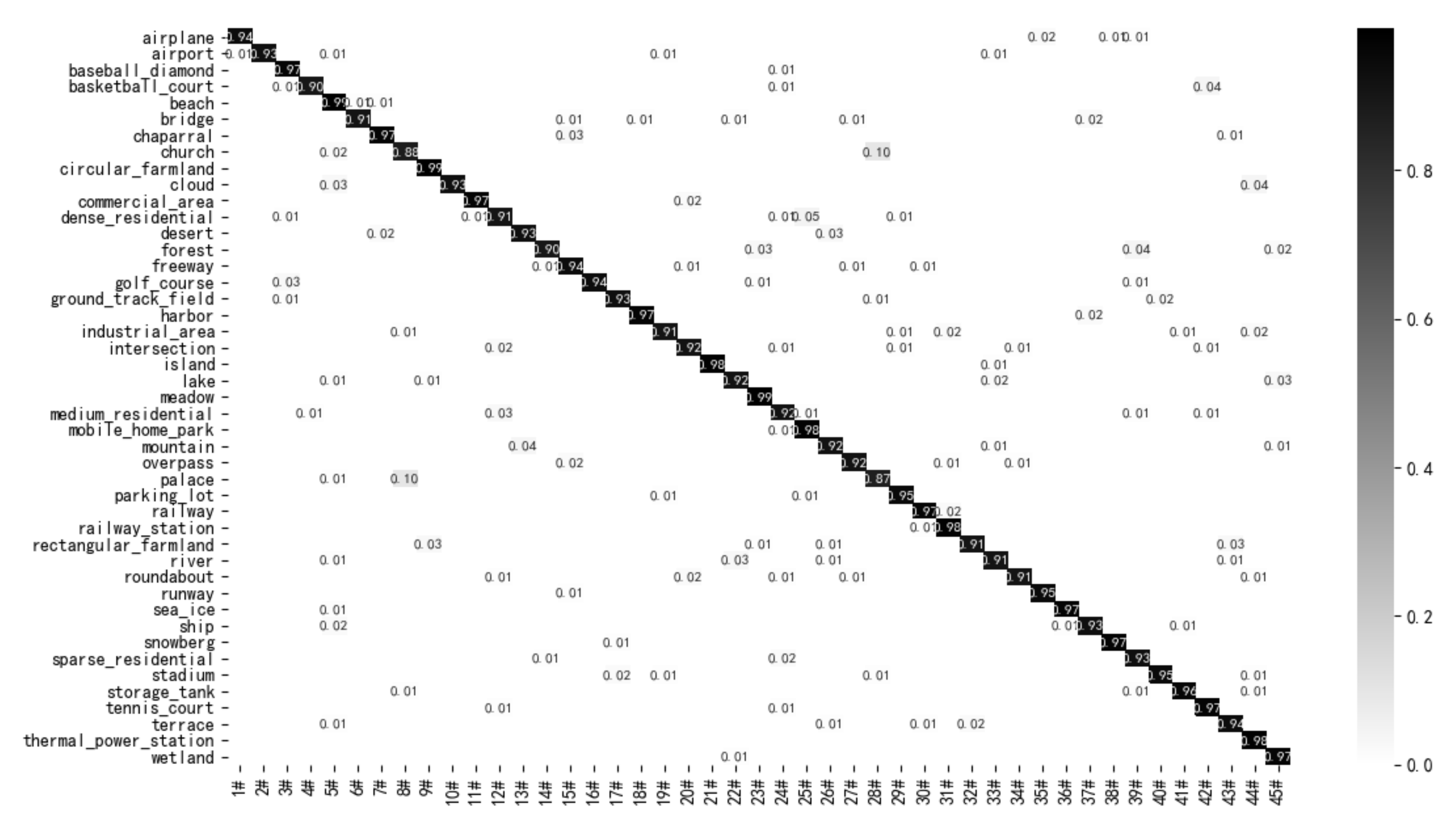
On the NWPU45 dataset, when training:test = 2:8, the confusion matrix obtained by the proposed LCNN-GWHA method is shown in Figure 9. Because the NWPU45 dataset contains rich content variations and a complex spatial structure, there are no fully recognized scenes when classifying the dataset. However, the classification accuracy of the proposed method for 43 scenes reached more than 90%. The lowest classification accuracy was for ‘palace’ and ‘church’, which were 87% and 88%, respectively. The main reason is that the two scenarios, ‘palace’ and ‘church’, have similar architectural styles and are easy to confuse when extracting features, resulting in classification errors.

3.4. Comparison of the Computational Complexity of Models

In addition, to further demonstrate the advantages of the proposed methods in terms of speed, MobileNetV2 [12], CaffeNet [23], VGG-VD-16 [23], GoogleNet [23], Contourlet CNN [26], SE-MDPMNet [29], Inception V3 [46], ResNet50 [46], LiG with RBF kernel [51], and LGRIN [53] were used for comparison with the proposed LCNN-CMGF method. Some experiments were carried out on the AID dataset. The size of Giga Multiply-Accumulation operations per second (GMACs) was used as the evaluation index in the experiments. The GMACs measures the computational complexity of a model. The comparison of experimental results of these methods on the AID dataset with training:test = 5:5 is shown in Table 11. As shown in Table 11, the OA of the proposed LCNN-CMGF method is 97.54%, the parameter quantity is 0.8 M, and the GMACs value is 0.0160 G. Compared with other lightweight models LiG with RBF kernel [51] and MobleNetV2 [12], the proposed method achieves higher classification accuracy with less than half of the parameters of the two methods. Although the accuracy is slightly lower than that of LGRIN [53], the number of parameters is 3.83 M less than that of LGRIN [53], and the GMACs value is 0.4773 G less than that of LGRIN [53]. The proposed LCNN-CMGF method achieves a good trade-off between model complexity and classification accuracy.

3.5. Comparison Results of Shallow Feature Extraction Modules

Convolutional neural network first extracts the shallow feature of images. With the deepening of the network, the extracted features are more abstract and contain more semantic content, as shown in Figure 10. Figure 10a is the original remote sensing scene image. After the feature extraction of convolutional neural network, the shallow feature map is shown in Figure 10b. With the deepening of the network, more complex features are extracted, as shown in Figure 10c. Compared with the features in Figure 10b, the features in Figure 10c are more complex and have more semantic information. For the classification of remote sensing images, both shallow and deep features are very useful. The traditional methods for extracting shallow features of images are shown in Figure 2a,b. The two methods are not sufficient to extract the shallow features of the image, and some information will be lost during the feature extraction process. Therefore, we propose a three-branch downsampling structure to extract the shallow features of images. The three-branch downsampling structure has great performance advantages compared with the traditional convolution method. In order to prove the effectiveness of the proposed three-branch downsampling structure, the feature extraction capabilities of the two traditional downsampling structures (as shown in Figure 2a,b) and the proposed three-branch downsampling structure (as shown in Figure 3) are experimentally compared. The comparison process is as follows. In the first experiment, the downsampling structure in Figure 2a is used to replace the three-branch downsampling structure in group 1 and group 2 ofthe proposed method, represented by method 1. In the second experiment, the downsampling structure in Figure 2b is used to replace the three-branch downsampling structure in group 1 and group 2 of the proposed method, represented by method 2. In the third experiment, the three-branch downsampling structure is preserved, which was represented by method 3. The specific experimental parameter settings are shown in Section 2.2. Some comparative experiments were conducted on the AID dataset with training:test = 5:5. For a fair comparison, the three experiments were carried out under the same experimental conditions. The experimental results are listed in Table 12. As shown in Table 12, the three methods have no obvious difference in parameter quantity and model complexity. However, compared with method 3, the other two methods have lower classification accuracy. Specifically, the classification accuracy of method 3 is 1.08% and 1.57% higher than that of method 1 and method 2, respectively.

3.6. Ablation Experiment

In this section, the effectiveness of the number of channels of each group in a channel multi-group fusion structure on network performance is analyzed. Firstly, the group with 2/C channels of the designed multi-grouping fusion structure is removed, and then the structure diagram with channel number C/4 is obtained, which is shown in Figure 11a. Secondly, the group with C/4 channels of the designed multi-grouping fusion structure is removed, and then the structure diagram with channel number C/2 is obtained, which is shown in Figure 11b. Finally, the complete multi-group fusion structure is used for comparison. Some comparative experiments were conducted on the AID dataset with a training proportion of 50%. OA, parameters and GMACs were adopted as evaluation indexes in the experiment. In the three experiments, to make a fair comparison, the experimental equipment and experimental parameter settings are all the same. The experimental results are listed in Table 13. As shown in Table 13, when the grouping structure with the number of channels C/4 is adopted, as shown in Figure 11a, the OA is 96.09%, the parameter quantity is 0.57 M, and the GMACs value is 0.0153 G. When the grouping structure with the number of channels C/2 is adopted, as shown in Figure 11b, the OA is 95.20%, the parameter quantity is 0.53 M, and the GMACs value is 0.0149 G. The two structures are similar in parameter quantity and model complexity, but the OA of the grouping structure with channel number C/4 is higher than that of the grouping structure with channel number C/2 because it increases the diversity of features. However, there is still a large gap in classification performance between the two methods and the proposed multi-group fusion structure, which further proves the effectiveness of the proposed method.

4. Discussions

In order to display the feature extraction ability of the proposed method more intuitively, a series of visualization methods are adopted to evaluate the proposed method. Firstly, the feature extraction ability of the proposed method is presented by using the visualization method of Class Activation Map (CAM). The CAM method displays important areas of the image predicted by the model by generating a rough attention map from the last layer of the convolutional neural network. Some images in the UCM21 dataset are chosen for visualization experiments, and the visualization results are shown in Figure 12. As shown in Figure 12, the proposed LCNN-CMGF method can highlight semantic objects corresponding to real categories. This shows that the proposed LCNN-CMGF method has a strong ability to locate and recognize objects. In addition, the proposed LCNN-CMGF method can better cover semantic objects and has a wide highlight range.
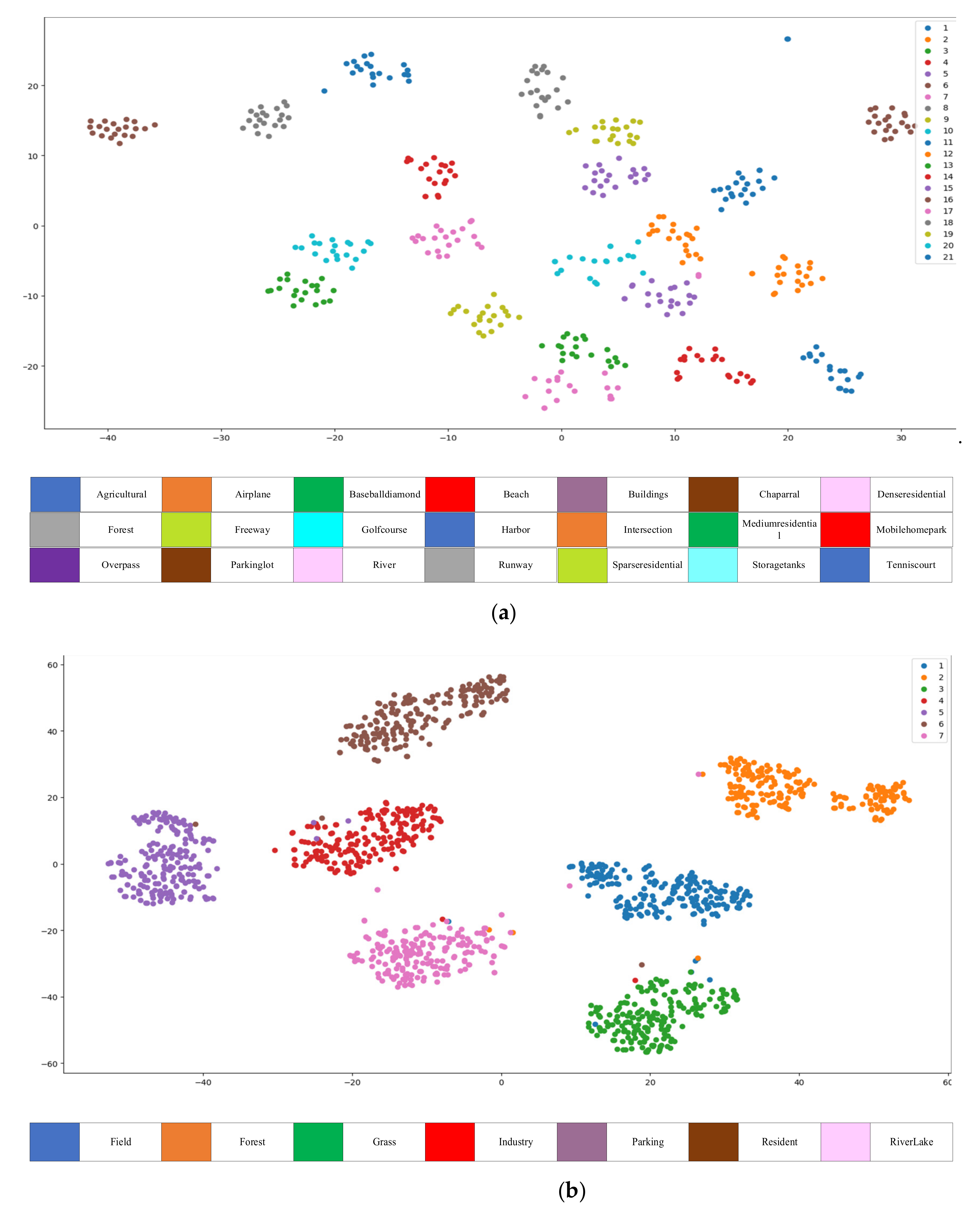
Next, t-distributed stochastic neighbor embedding visualization (T-SNE) method is used to visualize the proposed LCNN-CMGF method and further evaluate the performance of the proposed LCNN-CMGF method. T-SNE is a nonlinear dimensionality reduction algorithm, which usually maps high dimensions to two-dimensional or three-dimensional space for visualization, which can well evaluate the classification effect of the model. The RSSCN7 and UCM21 datasets are used for visualization experiments, and the experimental results are shown in Figure 13.
As shown in Figure 13, there is no confusion between single semantic clusters on the UCM21 dataset and the RSSCN7 dataset, which means that the proposed LCNN-CMGF method has better global feature representation, increases the separability and relative distance between single semantic clusters, and can more accurately extract the features of remote sensing scene images and improve the classification accuracy.
In addition, a randomized prediction experiment is performed on the UCM21 dataset using the LCNN-CMGF method. The results are shown in Figure 14. From Figure 14, we can see that the LCNN-CMGF method has more than 99% confidence in remote sensing image prediction, and some of the predictions even reach 100%. This further proves the validity of the proposed method for remote sensing scene image classification.
5. Conclusions

In this paper, a lightweight convolutional neural network based on channel multi-group fusion (LCNN-CMGF) was proposed to classify remote sensing scene images. In the proposed LCNN-CMGF method, the three-branch downsampling structure was designed to extract shallow features from remote sensing images. Channel multi-group fusion structure was presented to efficiently extract deep and abstract features of remote sensing images. The channel multi-group fusion structure utilizes channel fusion of adjacent features to reduce the lack of information exchange between groups caused by group convolution. The experimental results show that the proposed LCNN-CMGF method can achieve higher classification accuracy with fewer parameters and computational complexity than some state-of-the-art methods. Especially on UCM21 datasets, the OA value of this method is as high as 99.52%, which surpasses most of the existing advanced methods. Future work is to find a more effective convolution method to reduce the loss of feature information as much as possible while preserving the lightweight of the network.

Author Contributions

Conceptualization, C.S.; data curation, C.S. and X.Z.; formal analysis, L.W.; methodology, C.S.; software, X.Z.; validation, C.S. and X.Z.; writing—original draft, X.Z.; writing—review and editing, C.S. and L.W. All authors have read and agreed to the published version of the manuscript.

Funding

This research was funded in part by the National Natural Science Foundation of China (41701479, 62071084), in part by the Heilongjiang Science Foundation Project of China under Grant LH2021D022, and in part by the Fundamental Research Funds in Heilongjiang Provincial Universities of China under Grant 135509136.

Institutional Review Board Statement

Not applicable.

Informed Consent Statement

Not applicable.

Data Availability Statement

Data associated with this research are available online. The UC Merced dataset is available for download at http://weegee.vision.ucmerced.edu/datasets/landuse.html. RSCCN dataset is available for download at https://sites.google.com/site/qinzoucn/documents. NWPU dataset is available for download at http://www.escience.cn/people/JunweiHan/NWPU-RESISC45.html. AID dataset is available for download at https://captain-whu.github.io/AID/ (accessed on 15 December 2021).

Acknowledgments

We would like to thank the handling editor and the anonymous reviewers for their careful reading and helpful remarks.

Conflicts of Interest

The authors declare no conflict of interest.

References

  1. Jaiswal, R.K.; Saxena, R.; Mukherjee, S. Application of remote sensing technology for land use/land cover change analysis. J. Indian Soc. Remote Sens. 1999, 27, 123–128. [Google Scholar] [CrossRef]
  2. Chova, L.G.; Tuia, D.; Moser, G.; Valls, G.C. Multimodal classification of remote sensing images: A review and future directions. IEEE Proc. 2015, 103, 1560–1584. [Google Scholar] [CrossRef]
  3. Cheng, G.; Zhou, P.; Han, J. Learning Rotation-Invariant Convolutional Neural Networks for Object Detection in VHR Optical Remote Sensing Images. IEEE Trans. Geosci. Remote Sens. 2016, 54, 7405–7415. [Google Scholar] [CrossRef]
  4. Zhang, L.; Zhang, L.; Du, B. Deep learning for remote sensing data: A technical tutorial on the state-of-the-art. IEEE Geosci. Remote Sens. Mag. 2016, 4, 22–40. [Google Scholar] [CrossRef]
  5. Feng, J.; Li, D.; Gu, J.; Cao, X.; Shang, R.; Zhang, X.; Jiao, L. Deep Reinforcement Learning for Semisupervised Hyperspectral Band Selection. IEEE Trans. Geosci. Remote Sens. 2021, 1–19. [Google Scholar] [CrossRef]
  6. Girshick, R.; Donahue, J.; Darrell, T.; Malik, J. Rich Feature Hierarchies for Accurate Object Detection and Semantic Segmentation. In Proceedings of the 2014 IEEE Conference on Computer Vision and Pattern Recognition (CVPR), Columbus, OH, USA, 23–28 June 2014; pp. 580–587. [Google Scholar]
  7. Li, Y.; Wang, Q.; Liang, X.; Jiao, L. A Novel Deep Feature Fusion Network for Remote Sensing Scene Classification. In Proceedings of the IGARSS 2019—2019 IEEE International Geoscience and Remote Sensing Symposium, Yokohama, Japan, 28 July–2 August 2019; pp. 5484–5487. [Google Scholar]
  8. Zhao, B.; Zhong, Y.; Xia, G.-S.; Zhang, L. Dirichlet-Derived Multiple Topic Scene Classification Model for High Spatial Resolution Remote Sensing Imagery. IEEE Trans. Geosci. Remote Sens. 2016, 54, 2108–2123. [Google Scholar] [CrossRef]
  9. Wang, Q.; Liu, S.; Chanussot, J.; Li, X. Scene Classification with Recurrent Attention of VHR Remote Sensing Images. IEEE Trans. Geosci. Remote Sens. 2019, 57, 1155–1167. [Google Scholar] [CrossRef]
  10. Iandola, F.N.; Han, S.; Moskewicz, M.W.; Ashraf, K.; Dally, W.J.; Keutzer, K. Squeezenet: Alexnet-level accuracy with 50× fewer parameters and <1 mb model size. arXiv 2016, arXiv:1602.07360. [Google Scholar]
  11. Howard, A.G.; Zhu, M.; Chen, B.; Kalenichenko, D.; Wang, W.; Weyand, T.; Andreetto, M.; Adam, H. Mobilenets: Efficient convolutional neural networks for mobile vision applications. arXiv 2017, arXiv:1704.04861. [Google Scholar]
  12. Sandler, M.; Howard, A.; Zhu, M.; Zhmoginov, A.; Chen, L. MobileNetV2: Inverted residuals and linear bottlenecks. In Proceedings of the IEEE/CVF Conference on Computer Vision and Pattern Recognition (CVPR), Salt Lake City, UT, USA, 18–23 June 2018; pp. 4510–4520. [Google Scholar] [CrossRef] [Green Version]
  13. Hu, J.; Shen, L.; Sun, G. Squeeze-and-Excitation Networks. In Proceedings of the IEEE Conference on Computer Vision and Pattern Recognition (CVPR), Salt Lake City, UT, USA, 18–23 June 2018; pp. 7132–7141. [Google Scholar]
  14. Li, Y.; Jin, X.; Mei, J.; Lian, X.; Yang, L.; Xie, C.; Yu, Q.; Zhou, Y.; Bai, S.; Yuille, A.L. Neural Architecture Search for Lightweight Non-Local Networks. In Proceedings of the CVPR, IEEE Computer Society Conference on Computer Vision and Pattern Recognition, Seattle, WA, USA, 14–19 June 2020; pp. 10294–10303. [Google Scholar] [CrossRef]
  15. Howard, A.; Sandler, M.; Chen, B.; Wang, W.; Chen, L.-C.; Tan, M.; Chu, G.; Vasudevan, V.; Zhu, Y.; Pang, R.; et al. Searching for MobileNetV3. In Proceedings of the International Conference on Computer Vision, Seoul, Korea, 27 October–2 November 2019; pp. 1314–1324. [Google Scholar] [CrossRef]
  16. He, K.; Zhang, X.; Ren, S.; Sun, J. Identity Mappings in Deep Residual Networks. In Proceedings of the 14th European Conference on Computer Vision, Amsterdam, The Netherlands, 11–14 October 2016; pp. 630–645. [Google Scholar] [CrossRef] [Green Version]
  17. Chollet, F. Xception: Deep learning with depthwise separable convolutions. In Proceedings of the IEEE Conference on Computer Vision and Pattern Recognition (CVPR), Honolulu, HI, USA, 21–26 July 2017; pp. 1800–1807. [Google Scholar] [CrossRef] [Green Version]
  18. Szegedy, C.; Liu, W.; Jia, Y.; Sermanet, P.; Reed, S.; Anguelov, D.; Erhan, D.; Vanhoucke, V.; Rabinovich, A. Going deeper with convolutions. In Proceedings of the 2015 IEEE Conference on Computer Vision and Pattern Recognition (CVPR), Boston, MA, USA, 7–12 June 2015. [Google Scholar]
  19. Krizhevsky, A.; Sutskever, I.; Hinton, G.E. ImageNet classification with deep convolutional neural networks. Commun. ACM 2017, 60, 84–90. [Google Scholar] [CrossRef]
  20. Xie, S.N.; Girshick, R.; Dollar, P.; Tu, Z.W.; He, K.M. Aggregated Residual Transformations for Deep Neural Networks. In Proceedings of the IEEE Conference on Computer Vision and Pattern Recognition (CVPR), Honolulu, HI, USA, 21–26 July 2017; pp. 5987–5995. [Google Scholar] [CrossRef] [Green Version]
  21. Yang, Y.; Newsam, S. Bag-of-visual-words and spatial extensions for land-use classification. In Proceedings of the 18th SIGSPATIAL International Conference on Advances in Geographic Information Systems, San Jose, CA, USA, 3–5 November 2010; pp. 270–279. [Google Scholar] [CrossRef]
  22. Zou, Q.; Ni, L.; Zhang, T.; Wang, Q. Deep Learning Based Feature Selection for Remote Sensing Scene Classification. IEEE Geosci. Remote Sens. Lett. 2015, 12, 2321–2325. [Google Scholar] [CrossRef]
  23. Xia, G.-S.; Hu, J.; Hu, F.; Shi, B.; Bai, X.; Zhong, Y.; Zhang, L.; Lu, X. AID: A Benchmark Data Set for Performance Evaluation of Aerial Scene Classification. IEEE Trans. Geosci. Remote Sens. 2017, 55, 3965–3981. [Google Scholar] [CrossRef] [Green Version]
  24. Cheng, G.; Han, J.; Lu, X. Remote Sensing Image Scene Classification: Benchmark and State of the Art. Proc. IEEE. 2017, 105, 1865–1883. [Google Scholar] [CrossRef] [Green Version]
  25. Xu, C.; Zhu, G.; Shu, J. Robust Joint Representation of Intrinsic Mean and Kernel Function of Lie Group for Remote Sensing Scene Classification. IEEE Geosci. Remote Sens. Lett. 2021, 18, 796–800. [Google Scholar] [CrossRef]
  26. Liu, M.; Jiao, L.; Liu, X.; Li, L.; Liu, F.; Yang, S. C-CNN: Contourlet Convolutional Neural Networks. IEEE Trans. Neural Networks Learn. Syst. 2021, 32, 2636–2649. [Google Scholar] [CrossRef] [PubMed]
  27. Pan, H.; Pang, Z.; Wang, Y.; Wang, Y.; Chen, L. A New Image Recognition and Classification Method Combining Transfer Learning Algorithm and MobileNet Model for Welding Defects. IEEE Access 2020, 8, 119951–119960. [Google Scholar] [CrossRef]
  28. Pour, A.M.; Seyedarabi, H.; Jahromi, S.H.A.; Javadzadeh, A. Automatic Detection and Monitoring of Diabetic Retinopathy Using Efficient Convolutional Neural Networks and Contrast Limited Adaptive Histogram Equalization. IEEE Access 2020, 8, 136668–136673. [Google Scholar] [CrossRef]
  29. Zhang, B.; Zhang, Y.; Wang, S. A Lightweight and Discriminative Model for Remote Sensing Scene Classification with Multidilation Pooling Module. IEEE J. Sel. Top. Appl. Earth Obs. Remote Sens. 2019, 12, 2636–2653. [Google Scholar] [CrossRef]
  30. Zhang, W.; Tang, P.; Zhao, L. Remote sensing image scene classification using CNN-CapsNet. Remote Sens. 2019, 11, 494. [Google Scholar] [CrossRef] [Green Version]
  31. Liu, B.-D.; Meng, J.; Xie, W.-Y.; Shao, S.; Li, Y.; Wang, Y. Weighted Spatial Pyramid Matching Collaborative Representation for Remote-Sensing-Image Scene Classification. Remote Sens. 2019, 11, 518. [Google Scholar] [CrossRef] [Green Version]
  32. Zhang, D.; Li, N.; Ye, Q. Positional Context Aggregation Network for Remote Sensing Scene Classification. IEEE Geosci. Remote Sens. Lett. 2019, 17, 943–947. [Google Scholar] [CrossRef]
  33. Shi, C.; Wang, T.; Wang, L. Branch Feature Fusion Convolution Network for Remote Sensing Scene Classification. IEEE J. Sel. Top. Appl. Earth Obs. Remote Sens. 2020, 13, 5194–5210. [Google Scholar] [CrossRef]
  34. Li, J.; Lin, D.; Wang, Y.; Xu, G.; Zhang, Y.; Ding, C.; Zhou, Y. Deep Discriminative Representation Learning with Attention Map for Scene Classification. Remote Sens. 2020, 12, 1366. [Google Scholar] [CrossRef]
  35. He, N.; Fang, L.; Li, S.; Plaza, J.; Plaza, A. Skip-Connected Covariance Network for Remote Sensing Scene Classification. IEEE Trans. Neural Netw. Learn. Syst. 2019, 31, 1461–1474. [Google Scholar] [CrossRef] [PubMed] [Green Version]
  36. Sun, H.; Li, S.; Zheng, X.; Lu, X. Remote Sensing Scene Classification by Gated Bidirectional Network. IEEE Trans. Geosci. Remote Sens. 2020, 58, 82–96. [Google Scholar] [CrossRef]
  37. Lu, X.; Sun, H.; Zheng, X. A Feature Aggregation Convolutional Neural Network for Remote Sensing Scene Classification. IEEE Trans. Geosci. Remote Sens. 2019, 57, 7894–7906. [Google Scholar] [CrossRef]
  38. Li, B.; Su, W.; Wu, H.; Li, R.; Zhang, W.; Qin, W.; Zhang, S. Aggregated Deep Fisher Feature for VHR Remote Sensing Scene Classification. IEEE J. Sel. Top. Appl. Earth Obs. Remote Sens. 2019, 12, 3508–3523. [Google Scholar] [CrossRef]
  39. Yu, D.; Guo, H.; Xu, Q.; Lu, J.; Zhao, C.; Lin, Y. Hierarchical Attention and Bilinear Fusion for Remote Sensing Image Scene Classification. IEEE J. Sel. Top. Appl. Earth Obs. Remote Sens. 2020, 13, 6372–6383. [Google Scholar] [CrossRef]
  40. Alhichri, H.; Alswayed, A.S.; Bazi, Y.; Ammour, N.; Alajlan, N.A. Classification of Remote Sensing Images Using EfficientNet-B3 CNN Model with Attention. IEEE Access 2021, 9, 14078–14094. [Google Scholar] [CrossRef]
  41. Cao, R.; Fang, L.; Lu, T.; He, N. Self-Attention-Based Deep Feature Fusion for Remote Sensing Scene Classification. IEEE Geosci. Remote Sens. Lett. 2021, 18, 43–47. [Google Scholar] [CrossRef]
  42. Yan, P.; He, F.; Yang, Y.; Hu, F. Semi-Supervised Representation Learning for Remote Sensing Image Classification Based on Generative Adversarial Networks. IEEE Access 2020, 8, 54135–54144. [Google Scholar] [CrossRef]
  43. Zhao, F.; Mu, X.; Yang, Z.; Yi, Z. A novel two-stage scene classification model based on feature variable significance in high-resolution remote sensing. Geocarto Int. 2019, 35, 1–12. [Google Scholar] [CrossRef]
  44. Liu, Y.; Liu, Y.; Ding, L. Scene classification based on two-stage deep feature fusion. IEEE Geosci. Remote Sens. Lett. 2018, 15, 183–186. [Google Scholar] [CrossRef]
  45. Cheng, G.; Yang, C.; Yao, X.; Guo, L.; Han, J. When Deep Learning Meets Metric Learning: Remote Sensing Image Scene Classification via Learning Discriminative CNNs. IEEE Trans. Geosci. Remote Sens. 2018, 56, 2811–2821. [Google Scholar] [CrossRef]
  46. Li, W.; Wang, Z.; Wang, Y.; Wu, J.; Wang, J.; Jia, Y.; Gui, G. Classification of High-Spatial-Resolution Remote Sensing Scenes Method Using Transfer Learning and Deep Convolutional Neural Network. IEEE J. Sel. Top. Appl. Earth Obs. Remote Sens. 2020, 13, 1986–1995. [Google Scholar] [CrossRef]
  47. Lu, X.; Ji, W.; Li, X.; Zheng, X. Bidirectional adaptive feature fusion for remote sensing scene classification. Neurocomputing 2019, 328, 135–146. [Google Scholar] [CrossRef]
  48. Wang, S.; Guan, Y.; Shao, L. Multi-Granularity Canonical Appearance Pooling for Remote Sensing Scene Classification. IEEE Trans. Image Process. 2020, 29, 5396–5407. [Google Scholar] [CrossRef] [PubMed] [Green Version]
  49. Yu, Y.; Liu, F. A Two-Stream Deep Fusion Framework for High-Resolution Aerial Scene Classification. Comput. Intell. Neurosci. 2018, 2018, 1–13. [Google Scholar] [CrossRef] [Green Version]
  50. Xue, W.; Dai, X.; Liu, L. Remote Sensing Scene Classification Based on Multi-Structure Deep Features Fusion. IEEE Access 2020, 8, 28746–28755. [Google Scholar] [CrossRef]
  51. Xu, C.; Zhu, G.; Shu, J. A Lightweight Intrinsic Mean for Remote Sensing Classification with Lie Group Kernel Function. IEEE Geosci. Remote Sens. Lett. 2021, 18, 1741–1745. [Google Scholar] [CrossRef]
  52. Zhou, Y.; Liu, X.; Zhao, J.; Ma, D.; Yao, R.; Liu, B.; Zheng, Y. Remote sensing scene classification based on rotation-invariant feature learning and joint decision making. EURASIP J. Image Video Process. 2019, 1, 1–11. [Google Scholar] [CrossRef] [Green Version]
  53. Xu, C.; Zhu, G.; Shu, J. A Lightweight and Robust Lie Group-Convolutional Neural Networks Joint Representation for Remote Sensing Scene Classification. IEEE Trans. Geosci. Remote Sens. 2021, 60, 1–15. [Google Scholar] [CrossRef]
Figure 1. The proposed LCNN-CMGF network structure. Groups 1 and 2 are shallow downsampling modules. Group 3 is hybrid convolution. Groups 4–7 are channel multi-group fusion modules. Group 8 is the global average pooling, fc and classifier.
Remotesensing 14 00009 g001
Figure 2. The structure of traditional shallow sampling module. (a) Convolution downsampling. (b) Max-pooling downsampling.
Remotesensing 14 00009 g002
Figure 3. Three-branch shallow downsampling structure.
Remotesensing 14 00009 g003
Figure 4. Channel multi-group fusion structure.
Remotesensing 14 00009 g004
Figure 5. Different scene images in four datasets. (a) Scene images from the UCM21 dataset. (b) Scene images from the RSSCN7 dataset. (c) Scene images from the AID dataset. (d) Scene images from the NWPU45 dataset.
Remotesensing 14 00009 g005aRemotesensing 14 00009 g005bRemotesensing 14 00009 g005c
Figure 6. Confusion matrix of the LCNN-CMGF method on the UCM21 dataset (80/20).
Remotesensing 14 00009 g006
Figure 7. Confusion matrix of the LCNN-CMGF method on the RSSCN7 dataset (50/50).
Remotesensing 14 00009 g007
Figure 8. Confusion matrix of the LCNN-CMGF method on the AID (50/50) dataset.
Remotesensing 14 00009 g008
Figure 9. Confusion matrix of the LCNN-CMGF method on the NWPU45 (20/80) dataset.
Remotesensing 14 00009 g009
Figure 10. Visualization results of feature maps. (a) The original remote sensing scene image. (b) Visualization results of shallow features. (c) Visualization results of deep features.
Remotesensing 14 00009 g010
Figure 11. The proposed structure with different groups. (a) Structure diagram with channel number C/4. (b) Structure diagram with channel number C/2.
Remotesensing 14 00009 g011aRemotesensing 14 00009 g011b
Figure 12. Cam visualization results of the LCNN-CMGF method on the UCM21 dataset.
Remotesensing 14 00009 g012
Figure 13. T-SNE visual analysis results. (a) The T-SNE visualization results of the proposed method on UCM21 datasets. (b) The T-SNE visualization results of the proposed method on RSSCN7 datasets.
Remotesensing 14 00009 g013
Figure 14. Random classification prediction results.
Remotesensing 14 00009 g014
Table 1. Detailed description of four datasets.
DatasetsThe Number of Images per ClassThe Number of Scene CategoriesThe Total Number of ImagesThe Spatial Resolution of Images(m)Image Size
UCM211002121000.3256 × 256
RSSCN740072800-400 × 400
AID200–4003010,0000.5–0.8600 × 600
NWPU457004531,5000.2–30256 × 256
Table 2. Network architecture of the LCNN-CMGF method.
Input SizeGroupsOutput Size
256 × 256 × 31128 × 128 × 64
128 × 128 × 64264 × 64 × 128
64 × 64 × 128332 ×3 2 × 128
32 × 32 × 128416 × 16 × 128
16 × 16 × 12858 × 8 × 256
8 × 8 × 25668 × 8 × 256
8 × 8 × 25678 × 8 × 512
8 × 8 × 512Avgpooling1 × 1 × 512
1 × 1 × 512Dense1 × 1 × 7
Table 3. Experimental environment and parameter setting.
ItemContents
ProcessorAMD Ryzen 7 4800 H with Radeon [email protected] GHz
Memory16 G
Operating systemWindows10
Solid state hard disk512 G
SoftwarePyCharm Community Edition 2020.3.2
GPUNVIDIA GeForce RTX2060 6G
Kerasv2.2.5
Initial study rate0.01
Momentum0.9
Table 4. OA(%) of eighteen methods and the LCNN-CMGF method at the training ratio of 80% in the UCM21 dataset.
MethodOA(80%)Year
LiG with Sigmoid Kernel [25]98.92 ± 0.352020
Contourlet CNN [26]98.97 ± 0.212020
MobileNet [27]96.33 ± 0.152020
EfficientNet [28]94.37 ± 0.142020
Fine-Tune MobileNet V2 [29]98.13 ± 0.332019
VGG-16-CapsNet [30]98.81 ± 0.122019
ResNet + WSPM-CRC [31]97.952019
Positional Context Aggregation [32]99.21 ± 0.182020
LCNN-BFF Method [33]99.29 ± 0.242020
DDRL-AM Method [34]99.05 ± 0.082020
Skip-Connected CNN [35]98.04 ± 0.232020
Gated Bidirectiona + Global Feature [36]98.57 ± 0.482020
Feature Aggregation CNN [37]98.81 ± 0.242019
Aggregated Deep Fisher Feature [38]98.81 ± 0.512019
HABFNet [39]99.29 ± 0.352020
EfficientNetB3-Attn-2 [40]99.21 ± 0.222021
VGG_VD16 with SAFF [41]97.02 ± 0.782020
Semi-Supervised Representation Learning [42]94.05 ± 1.22020
Proposed99.52 ± 0.342021
Table 5. Kappa (%) of six methods and the LCNN-CMGF method at the training ratio of 80% in the UCM21 dataset.
MethodOA (80%)Kappa (%)
LiG with Sigmoid Kernel [25]98.92 ± 0.3597.63
Contourlet CNN [26]98.97 ± 0.2197.81
MobileNet [27]96.33 ± 0.1594.91
EfficientNet [28]94.37 ± 0.1493.37
Fine-Tune MobileNet V2 [29]98.1396.92
SE-MDPMNet [29]98.9597.74
Proposed99.52 ± 0.3499.50
Table 6. OA (%) of seven kinds of methods and the LCNN-CMGF method under the training ratios of 50% in the RSSCN7 dataset.
MethodOA (50%)Year
Contourlet CNN [26]95.54 ± 0.172020
VGG-16-CapsNet [30]96.65 ± 0.232019
SPM-CRC [31]93.862019
WSPM-CRC [31]93.602019
Positional Context Aggregation [32]95.98 ± 0.562020
ADFF [38]95.21 ± 0.502019
LCNN-BFF [33]94.64 ± 0.122020
SE-MDPMNet [29]92.46 ± 0.662019
Variable-Weighted Multi-Fusion [43]89.12019
Proposed97.50 ± 0.212021
Table 7. Kappa (%) of fourteen methods and the LCNN-CMGF method at the training ratio of 50% in the AID dataset.
MethodOA (20/80)(%) OA (50/50)(%)Year
MobileNet [27]88.53 ± 0.1790.91 ± 0.182020
EfficientNet [28]86.56 ± 0.1788.35 ± 0.162020
Feature Aggregation CNN [37]-95.45 ± 0.112019
TSDFF [44]-94.652018
Discriminative + AlexNet [45]85.62 ± 0.1094.47 ± 0.122018
InceptionV3 [46]93.27 ± 0.1795.07 ± 0.222020
Bidirectional Adaptive Feature Fusion [47]-93.562019
MG-CAP(Bilinear) [48]92.11 ± 0.1595.14 ± 0.122020
LCNN-BFF [33]92.06 ± 0.3694.53 ± 0.242020
DDRL-AM Method [34]91.56 ± 0.4994.08 ± 0.352020
GBNet [36]90.16 ± 0.2493.72 ± 0.342020
GBNet + Global Feature [36]92.20 ± 0.2395.48 ± 0.122020
Aggregated Deep Fisher Feature [38]92.78 ± 0.5795.26 ± 0.842019
HABFNet [39]93.01 ± 0.4396.75 ± 0.522020
EfficientNetB3-Attn-2 [40]92.48 ± 0.7695.39 ± 0.432021
VGG_VD16 with SAFF Method [41]92.05 ± 0.3495.98 ± 0.702020
ResNet50 [46]92.39 ± 0.1594.69 ± 0.192020
VGG19 [46]87.73 ± 0.2591.71 ± 0.242020
Skip-Connected CNN [35]91.10 ± 0.1593.30 ± 0.132020
Proposed93.63 ± 0.1097.54 ± 0.252021
Table 8. Kappa (%) of seven methods and the LCNN-CMGF method at the training ratios of 50% in the AID dataset.
MethodOA (50%)Kappa (%)
Two-Stage Deep Feature Fusion [44]94.6593.41
MobileNet [27]90.91 ± 0.1889.53
EfficientNet [28]88.35 ± 0.1687.21
Semi-Supervised Representation Learning [42]95.6395.50
TSDFF [44]94.6593.96
Discriminative + AlexNet [45]94.47 ± 0.1294.26
Variable-Weighted Multi-Fusion [43]96.23 ± 0.3596.12
Two-Stream Deep Fusion Framework [49]94.5893.34
InceptionV3 [46]95.07 ± 0.2294.83
ResNet50 [46]94.69 ± 0.1993.47
VGG19 [46]91.71 ± 0.2490.06
Proposed97.54 ± 0.2597.45
Table 9. OA (%) of seventeen methods and the LCNN-CMGF method at the training ratios of 20% and 10% in the NWPU45 dataset.
Network ModelOA (10/90)(%)OA (20/80)(%)Year
Contourlet CNN [26]85.93 ± 0.5189.57 ± 0.452020
MG-CAP with Biliner [48]89.42 ± 0.1991.72 ± 0.162020
EfficientNet [28]78.57 ± 0.1581.83 ± 0.152020
LiG with RBF Kernel [51]90.23 ± 0.1393.25 ± 0.122020
LiG with Sigmoid Kernel [25]90.19 ± 0.1193.21 ± 0.122020
VGG19 [46]81.34 ± 0.3283.57 ± 0.372020
ResNet50 [46]86.23 ± 0.4188.93 ± 0.122020
InceptionV3 [46]85.46 ± 0.3387.75 ± 0.432020
MobileNet [27]80.32 ± 0.1683.26 ± 0.172020
Discriminative + VGG16 [45]89.22 ± 0.5091.89 ± 0.222018
Discriminative + AlexNet [45]85.56 ± 0.2087.24 ± 0.122018
Skip-Connected CNN [35]84.33 ± 0.1987.30 ± 0.232020
LCNN-BFF Method [33]86.53 ± 0.1591.73 ± 0.172020
VGG-16-CapsNet [30]85.05 ± 0.1389.18 ± 0.142019
VGG_VD16 with SAFF Method [41]84.38 ± 0.1987.86 ± 0.142020
MSDFF [50]91.5693.552020
R.D [52]-91.032019
Proposed92.53 ± 0.5694.18 ± 0.352021
Table 10. Kappa (%) of ten methods and the LCNN-CMGF method at the training ratio of 20% in the NWPU45 dataset.
Network ModelOA (20%)Kappa (%)
Contourlet CNN [26]89.57 ± 0.4588.35
EfficientNet [28]81.83 ± 0.1579.53
LiG with RBF Kernel [51]93.25 ± 0.1293.02
LiG with Sigmoid Kernel [25]93.2192.92
VGG19 [46]83.5782.17
ResNet50 [46]88.9387.61
InceptionV3 [46]87.7586.46
MobileNet [27]83.2681.72
Fine-Tune MobileNet V2 [29]93.0092.93
LCNN-BFF Method [33]91.7391.54
Proposed94.18 ± 0.3594.04
Table 11. Evaluation values of ten methods and the LCNN-CMGF method at the training ratio of 50% in the AID dataset.
MethodOA (%)ParametersGMACs
Contourlet CNN [26]89.5712.6 M1.0583 G
SE-MDPMNet [29]97.145.17 M0.9843 G
LiG with RBF Kernel [51]96.192.07 M0.2351 G
InceptionV3 [46]95.0745.37 M2.4356 G
ResNet50 [46]94.6925.61 M1.8555 G
MobileNetV2 [12]95.963.5 M0.3451 G
VGG-VD-16 [23]89.64138.36 M7.7500 G
CaffeNet [23]89.5360.97 M3.6532 G
GoogleNet [23]86.397 M0.7500 G
LGRIN [53]97.654.63 M0.4933 G
Proposed97.540.8 M0.0160 G
Table 12. Comparison results of feature extraction ability of three methods.
MethodOA(%)ParametersGMACs
method 196.46 ± 0.360.79 M0.0156 G
method 295.97 ± 0.160.77 M0.0152 G
method 397.54 ± 0.250.8 M0.0160 G
Table 13. Comparison results of the proposed structure with different groupings on network performance.
GroupOA(%)ParametersGMACs
4/C96.09 ± 0.610.57 M0.0153 G
2/C95.20 ± 0.150.53 M0.0149 G
2/C + 4/C97.54 ± 0.250.8 M0.0160 G
Publisher’s Note: MDPI stays neutral with regard to jurisdictional claims in published maps and institutional affiliations.