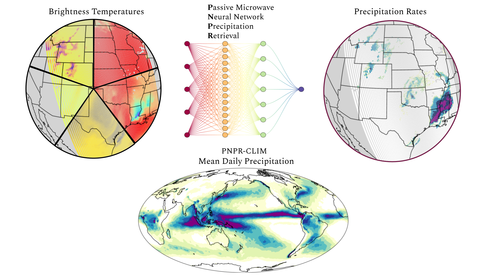
The Passive Microwave Neural Network Precipitation Retrieval Algorithm for Climate Applications (PNPR-CLIM): Design and Verification

Abstract

This paper describes the Passive microwave Neural network Precipitation Retrieval algorithm for climate applications (PNPR-CLIM), developed with funding from the Copernicus Climate Change Service (C3S), implemented by ECMWF on behalf of the European Union. The algorithm has been designed and developed to exploit the two cross-track scanning microwave radiometers, AMSU-B and MHS, towards the creation of a long-term (2000–2017) global precipitation climate data record (CDR) for the ECMWF Climate Data Store (CDS). The algorithm has been trained on an observational dataset built from one year of MHS and GPM-CO Dual-frequency Precipitation Radar (DPR) coincident observations. The dataset includes the Fundamental Climate Data Record (FCDR) of AMSU-B and MHS brightness temperatures, provided by the Fidelity and Uncertainty in Climate data records from Earth Observation (FIDUCEO) project, and the DPR-based surface precipitation rate estimates used as reference. The combined use of high quality, calibrated and harmonized long-term input data (provided by the FIDUCEO microwave brightness temperature Fundamental Climate Data Record) with the exploitation of the potential of neural networks (ability to learn and generalize) has made it possible to limit the use of ancillary model-derived environmental variables, thus reducing the model uncertainties’ influence on the PNPR-CLIM, which could compromise the accuracy of the estimates. The PNPR-CLIM estimated precipitation distribution is in good agreement with independent DPR-based estimates. A multiscale assessment of the algorithm’s performance is presented against high quality regional ground-based radar products and global precipitation datasets. The regional and global three-year (2015–2017) verification analysis shows that, despite the simplicity of the algorithm in terms of input variables and processing performance, the quality of PNPR-CLIM outperforms NASA GPROF in terms of rainfall detection, while in terms of rainfall quantification they are comparable. The global analysis evidences weaknesses at higher latitudes and in the winter at mid latitudes, mainly linked to the poorer quality of the precipitation retrieval in cold/dry conditions.

1. Introduction

In 2016, the European Centre for Medium-Range Weather Forecasts (ECMWF) implemented the Copernicus Climate Change Service (C3S), on behalf of the European Union, aimed at producing a new set of Essential Climate Variables (ECVs, variables that critically contribute to the characterization of the Earth’s climate) from observations (https://climate.copernicus.eu/c3s312b-essential-climate-variable-products-derived-observations, accessed on 12 February 2021). The project focuses on five different variable categories, related to atmospheric physics (Lot 1), atmospheric composition (Lot 2), ocean (Lot 3), land hydrology and cryosphere (Lot 4) and land biosphere (Lot 5). Lot 1 contains precipitation as an essential climatic variable. Indeed, precipitation plays a crucial role in the global hydrological and energy cycles and therefore in many activities, such as agriculture, management of water resources and natural hazards, weather and hydrological predictions. Accurate global measurements of precipitation are important for these reasons and for understanding the natural variability of the Earth’s climate [1,2,3,4,5,6,7,8,9].

In this context, satellite borne sensors, providing global observations, play a key role in estimating precipitation, while ground-based measurements provided by rain gauges and radars have limited coverage [6,9,10,11]. Microwave (MW) sensors, in particular, are essential for the space-based precipitation measurements as, unlike infrared and visible instruments, directly respond to the absorption and scattering of cloud hydrometers (e.g., [2,12,13,14,15,16]). Opaque channels around 183 GHz, for example, originally designed to retrieve water vapor distribution due to their different sensitivity to specific layers of the atmosphere [17,18,19], have shown great potential for precipitating cloud characterization and for precipitation retrieval. In fact, the different penetration properties of these frequency channels in the atmosphere can be exploited to analyze the vertical distribution of hydrometeors [17,18,20,21,22,23,24,25,26] and to obtain some criteria for the characterization of precipitation (weak, moderate, strong convective and stratiform, for example, [27,28]).

The Passive microwave Neural network Precipitation Retrieval algorithm for climate applications (PNPR-CLIM) described in this paper, has been designed and developed to exploit the two cross-track scanning passive microwave radiometers, Advanced Microwave Sounding Unit-B (AMSU-B) and Microwave Humidity Sounder (MHS) long-term measurements to contribute to the global precipitation climate data record (CDR) to be released in collaboration with Deutscher Wetterdienst (DWD) within the C3S program. Neural Networks (NNs) represent a highly flexible ensemble of non-linear and non-parametric regression and classification statistical models, widely applied in many fields of the Environmental Sciences for their capability to approximate complex non-linear and imperfectly known functions to various degrees of accuracy [19,29,30]. The opportunities offered by their ability to learn and generalize, as well as to be quite robust to handle noise in the input variables, have encouraged their use in precipitation estimation from satellite and ground measurements. This technique has proven to be effective in this area of research and were successfully used in many rainfall estimation and monitoring applications [31,32,33,34,35,36,37,38]. By definition, NN models [35] are supervised learning algorithms and, as such, their design requires a training phase in which the model parameters are chosen to model an empirical function of some sample data (the training dataset). In the precipitation retrieval context, this translates into a sample of radiometric and ancillary input states, together with the actual precipitation rates linked to them. It is worth noting that the performance of the NN is largely dependent on the training dataset completeness and representativeness, and on its consistency with the actual observations. Training datasets created by means of both cloud resolving model (CRM) coupled to radiative transfer models were used for a long a time [6,39,40,41,42,43]. They were also used in the previous version of the PNPR algorithms for AMSU/MHS [35] and for Advanced Technology Microwave Sounder (ATMS) [36] that are currently used to deliver operational regional products (mainly over Europe and Africa) within the EUMETSAT Satellite Application Facility for Operational Hydrology and Water Management (H SAF). There are, however, some limitations associated with the use of CRMs, such as uncertainties in surface property characterization (e.g., surface emissivity), single scattering properties of ice or mixed phase hydrometeors, cloud microphysics parameterizations (particle size distributions, bulk densities, conversion processes), vertical and horizontal distribution of solid and liquid hydrometeors [44,45,46]. These limitations, being essentially due to the complexity and variety of the real atmospheric states and cloud structures, can be partially overcome by considering purely observational training datasets, if available.

Since the launch of the Global Precipitation Measurement mission (GPM) on 28 Febuary 2014, an extended and high quality set of spaceborne radar precipitation measurements have become available [47,48,49]. The Dual-frequency Precipitation Radar (DPR) at Ku-band (13.6 GHz) and Ka-band (35.5 GHz) [50] on-board the NASA/JAXA GPM Core Observatory (GPM-CO) provides precipitation measurements, covering the globe from 67${}^{°}$ N to 67${}^{°}$ S. The high quality of DPR-based products is supported by several validation studies [51,52,53,54] and field campaigns [55,56].

Metrologically-robust Fundamental Climate Data Records (FCDRs), that is, long-term records of satellite measurements (top-of-atmosphere radiance, reflectance and brightness temperature (BT)), were developed within the “Fidelity and Uncertainty in Climate data records from Earth Observation (FIDUCEO)” project. FIDUCEO FCDRs consist of continuous, harmonised records of calibrated, geolocated, uncertainty-quantified microwave sensor observations [57,58,59,60,61]. Carefully calibrated and homogenized radiance datasets are a fundamental prerequisite in the development of an algorithm aimed at performing climate analysis and monitoring. Thus, to take advantage of the enhanced stability and consistency of the FIDUCEO FCDR, ideally preserved in the derived geophysical variables for climate applications, the PNPR-CLIM algorithm was trained with an observational dataset composed of global GPM DPR-based precipitation estimates coincident, in space and time, with the AMSU-B/MHS BT measurements. In the dataset, the DPR-based precipitation rate is coupled to the FIDUCEO FCDR BTs.

However, it should be noted that, despite the advantages of using entirely observational training datasets, some criticality remains. Indeed, the precipitation retrieval from multi-frequency microwave BTs (especially from radiometers equipped only with high-frequency channels as the MHS and AMSU-B) does not guarantee unique surface precipitation rate solution, as a given multi-channel radiometric observation may be associated to different precipitation profiles (this is the ambiguity, or ill-posed inverse problem). Therefore, without the knowledge of an approximate state of the atmosphere, this problem turns out to be hardly solvable. Bayesian algorithms, like the GPM’s Goddard Profiling Algorithm (GPROF, [41]), or the Cloud Radiation Dynamic Database approach [42,43,46,62] overcome this difficulty, to a certain degree, by drawing from a large a priori database only the precipitation profiles constrained by model-derived atmospheric conditions at the time closest to the satellite overpass. The most probable state associated with each new observation is then used to return the surface precipitation estimate. Of course, this implies a good confidence in the highly dependent ancillary variables used to constrain the searching scheme at each algorithm run, reducing the algorithm independence from the model reanalysis or prediction. Similarly, but with important peculiarities, PNPR-CLIM uses two kinds of ancillary, model-derived variables to tune its predictions—snow-cover and sea-ice fraction daily products on one side, and 2 m temperature, freezing level and total precipitable water monthly means, all provided by the ECMWF ERA5 global reanalysis [63]. The daily time resolution of the sea-ice and snow cover data was chosen to better represent these two highly variable fields. In fact, their extremely variable emissivity has a significant effects on the upwelling radiation (especially in dry conditions) and tends to contaminate the precipitation microwave signal [64,65,66,67]. The choice of low time resolutions (monthly) for the other ERA5 variables, instead, ensures the dominance of the instantaneous information (TBs) over the ancillary one, determining a weak dependence on other data sources. It is therefore a global training dataset, mostly based on GPM and AMSU/MHS coincident global observations, as required within the C3S project. The goal is to provide high quality satellite-based precipitation rate estimates using calibrated and harmonized long-term input data, reducing as far as possible the dependence on the uncertainties inherent in external datasets and/or models by exploiting in the best way the information provided by the satellite observations.

Besides the description of the algorithm design, training and preliminary verification phase (against an independent DPR coincidence database), this paper presents the result of PNPR-CLIM quality assessment at regional and global scales. At regional scale the verification examines the instantaneous (Level 2) precipitation rate, comparing the GPROF and PNPR-CLIM estimates with the Multi-Radar and Multi-Sensor (MRMS) system precipitation product over the CONtiguous U.S. region (CONUS). The global verification, instead, is carried out at daily scale using the Global Precipitation Climatology Project (GPCP) daily precipitation product for comparison [68,69,70].

The paper is structured as follows—in Section 2 the adopted material and methods, namely the general definitions, input data, reference products and analysis methodologies are reported and described. Then, in Section 3, the algorithm design and implementation are described. Section 4 contains the verification results and the discussion. This section includes a global verification over the DPR covered area, a regional validation over the CONUS area and global analysis of PNPR-CLIM and GPROF using GPCP. Finally, Section 5 is devoted to the conclusions.

2. Materials and Methods

2.1. Neural Networks

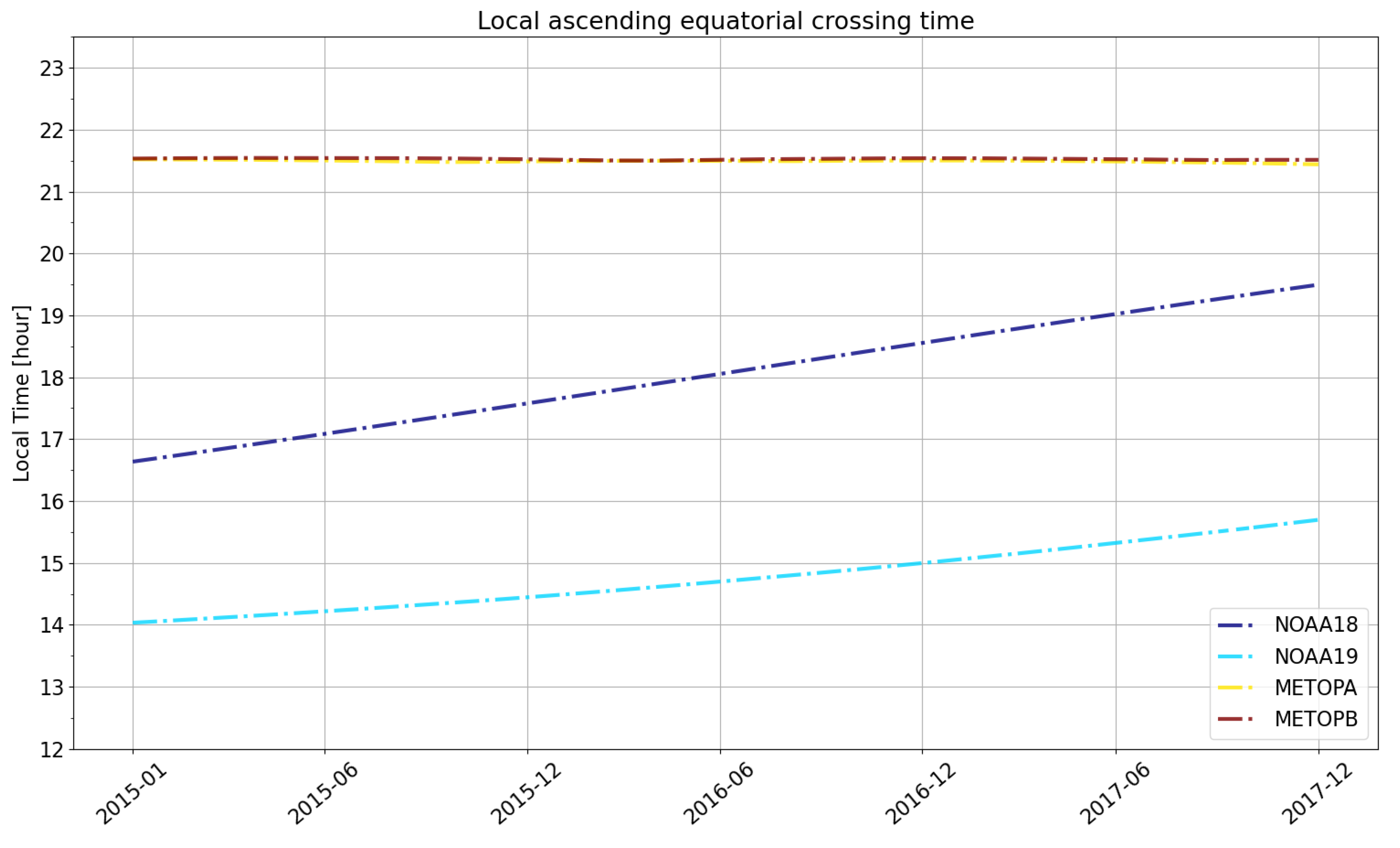
Generally, a NN consists of a number of neurons, arranged in different layers, which exchange information with each other. Each layer holds a number of neurons determined, along with the number of layers, during the design of the network. Each layer has its own (non-linear) transfer function and receives, as input, a linear transformation of the outputs of the previous layer. Therefore, the output of the l-th layer of a generic, fully-connected, NN turns out to be

$$y^{\left(l\right)}(x;{\omega }^{\left(1\right)},\dots ,{\omega }^{\left(l\right)})=\left\{\begin{array}{cc}{f}^{\left(l\right)}\left({\omega }^{\left(l\right)}·y^{(l-1)}\left(x;{\omega }^{\left(1\right)},\dots ,{\omega }^{(l-1)}\right)\right),\hfill & l>1,\hfill \\ f^{\left(1\right)}\left({\omega }^{\left(1\right)}·x\right),\hfill & l=1,\hfill \end{array}\right.$$

where, for $k=1,\dots ,l$, ${\omega }^{\left(k\right)}$ is the weight matrix of the $k-$th layer, $f^{\left(k\right)}$ is the activation function of the same layer, and x is the augmented input vector (i.e., the input vector embedded in a higher dimensional space by $(x^1,\dots ,x^m)\mapsto (x^1,\dots ,x^m,1)$).

The weights $\omega =({\omega }^{\left(1\right)},\dots ,{\omega }^{\left(l\right)})$ are optimal parameters, solution of the (local) optimization problem

$$\omega =\underset{{\omega }^{\prime }}{arg\; min}\mathcal{E}\left({\omega }^{\prime }\right),$$

for a suitable error function $\mathcal{E}$, commonly found throughout an iterative minimization scheme. Depending on the applications, a common choice of the error function, adopted also for PNPR-CLIM, is

$$\mathcal{E}=\left\{\begin{array}{cc}\frac{1}{n}\sum _{i=1}^n{(y_i-t_i)}^2,\hfill & \mathrm{for}\mathrm{regression},\hfill \\ \frac{1}{n}\sum _{i=1}^n\left(t_{i}log\left(y_i\right)+(1-t_i)log(1-y_i)\right),\hfill & \mathrm{for}\mathrm{binary}\mathrm{classification},\hfill \end{array}\right.$$

where n is the number of elements in the training set and $y_i=y(x_i;\omega )$ and $t_i=t\left(x_i\right)$ are the model prediction and real value, at the $i-$th sample $x_i$, of the variable t to modelize. A detailed description of the NN design process adopted for PNPR-CLIM can be found in [35,36,37].

2.2. Input Data

The PNPR-CLIM algorithm is based on the cross-track AMSU-B and MHS radiometers on board the NOAA and MetOp satellites, for the measurement of brightness temperatures at five frequencies (

Table 1. AMSU-B and MHS radiometers’ characteristics.

Satellites	AMSU-B: NOAA-15, NOAA-16, NOAA-17
	MHS: NOAA-18, NOAA-19, MetOp-A, MetOp-B, MetOp-C
MHS/AMSU-B Central Frequency (GHz)	MHS/AMSU-B Channel Bandwidth (MHz)	MHS/AMSU-B Channel Polarisation (Nadir)
89.0	2800/1000	V/V
157.0/150.0	2800/1000	V/V
183.31 ± 1.0	1000/500	H/V
183.31 ± 3.0	2000/1000	H/V
190.311/183.31 ± 7.0	2000/2000	V/V

). MHS channels are very similar to those of AMSU-B with the exception of channel 2 centered at 157 GHz and channel 5, which is a single passband channel centered at 190 GHz. Some differences are also present in the polarization of channels 3 and 4 that are horizontal for MHS and vertical for AMSU-B at nadir. The nominal resolution of AMSU-B and MHS varies with the cross-track scan angle from 16 × 16 km${}^2$ (circular) at nadir to 26 × 52 km${}^2$ (ovate) at scan edge. The regular 1.1${}^{°}$ sampling geometry of AMSU-B and MHS leads to a variable at-surface sampling distance, which corresponds to 16 km at nadir.

The BTs utilized in PNPR-CLIM are provided by FIDUCEO FCDR (v4.1). The FCDR file contains, for the MW sensor series aboard the NOAA and MetOp satellites, the calibrated BTs for each channel, its uncertainties categorised by their origin from independent, structured and common effects, and concise quality flags conveying helpful information on the usability of the data. It includes a period of more than twenty years (1994–2017) with a global spatial coverage. Despite the differences between the two radiometers, and the ones between different satellites, the inter-satellite and inter-instruments biases were understood and reduced by an improved calibration in the FIDUCEO FCDR [59]. Therefore, in this work we will refer to the AMSU-B/MHS FIDUCEO FCDR without specifying the instrument used for a given period. For PNPR-CLIM development activity (training and verification), a two-year (2015–2016) period was considered. The complete AMSU-B and MHS FCDR was used to produce the L2 precipitation rate estimate for the 18 year (2000–2017) period.

In addition to the FIDUCEO BTs, two kinds of ancillary data are associated to each radiometer pixel (i.e., to the BT vector). The first consists of ERA5 variables, precisely the daily sea-ice cover and snow-cover and the monthly mean of freezing level, total precipitable water, and 2 m temperature. The other consists of static variables, namely the AMSU-B/MHS cross-track scan angle of each observation, and the land type (either ocean, coast or land). The list of the PNPR-CLIM input variables is summarized in

Table 2. PNPR-CLIM input variables.

Variable	Type	Source
Brightness Temperatures	Instantaneous	FIDUCEO
Sea-ice cover	Daily	ERA5
Snow-cover	Daily	ERA5
Freezing level	Monthly	ERA5
Total precipitable water	Monthly	ERA5
2 m temperature	Monthly	ERA5
Scan angle	Static	FIDUCEO
Surface type map	Static	ESA

.

2.3. GPM-CO Dual-Frequency Precipitation Radar

For the development of the PNPR-CLIM algorithm, an observational dataset, built from time and space coincident GPM-CO DPR precipitation estimates (used as reference) and the AMSU-B/MHS BTs measurements, was used in the NNs training and verification phases.

The DPR is the second space-borne precipitation radar, following the Precipitation Radar (PR), launched on the TRMM satellite in November, 1997. The DPR consists of a Ku-band (13.6 GHz) and a Ka-band (35.5 GHz) radars (Iguchi, 2020). These Earth-pointing KuPR and KaPR instruments provide 3D precipitation measurements over all surfaces between 67${}^{°}$ N and 67${}^{°}$ S since March 2014. The KuPR and KaPR design specifications are shown in

Table 3. Summary of the characteristics of the GMP Dual-frequency Precipitation Radar (DPR). The GPM KuPR minimum threshold is closer to 12–13 dBZ than the official 18 dBZ in the table (from [71]).

Instrument	GPM DPR
Bands	KaPR	KuPR
Launch time	27 February 2014	27 February 2014
Altitude (km)	407	407
Inclination angle (°)	65	65
Frequencies (GHz)	35.547/35.553	13.597/13.603
Horizontal res. at nadir (km)	5.2	5.2
Swath width (km)	120	245
Vertical resolution (m)	250/500	250
Minimum detectable Ze (dBZ)	12 (KaHS)/18 (KaMS)	18
Measurement accuracy (dBZ)	<$\pm 1$	<$\pm 1$

.

2.4. Datasets and Products for the Quality Assessment

The quality assessment of PNPR-CLIM precipitation estimates involved several precipitation products and was carried out at regional and global scales. The description of the reference product and of the other satellite precipitation datasets used for comparison is provided in the following sections.

2.4.1. MRMS

The MRMS system incorporates observations from polarimetric radars (U.S. Next-Generation Radar (NEXRAD) network of 160 S-band polarimetric doppler (WSR-88D) radars, together with some of the Canadian radars), automated rain-gauge networks, lightning observations and forecast model predictions over CONUS. Data are produced by the National Oceanic and Atmospheric Administration (NOAA)’s National Severe Storms Laboratory (NSSL) jointly with the University of Oklahoma [68]. MRMS provides high quality gridded precipitation products over a 0.01° resolution regular horizontal grid, and 2 min temporal resolution, and is used as a benchmark for GPM precipitation products. In this study the radar-only precipitation rates (2 min temporal resolution, values in mm/h) and radar quality indices (2 min temporal resolution, values between 0, low quality, and 1, high quality) were considered. All the MRMS data used in this analysis are archived and freely disseminated by the Iowa State University, department of Geological and Atmospheric Sciences.

2.4.2. GPCP

The Global Precipitation Climatology Project (GPCP) provides global estimates of precipitation at daily resolution since 1996 on a 1° × 1° spatial grid [69,70]. The dataset is based on observations by microwave imagers on polar-orbiting satellites and infrared imagers on geostationary satellites. The data are made available via NOAA’s National Centers for Environmental Information and, since 2020, through the ECMWF Copernicus Climate Data Store (CDS). In this study the 1° × 1° daily product (mm/d), 1DD version v1.3 is used for the verification of PNPR-CLIM precipitation estimation at global scale.

2.4.3. GPROF

The Goddard PROFiling algorithm (GPROF) is a physically-based Bayesian precipitation retrieval algorithm used to deliver the official NASA GPM L2 precipitation products for all the GPM MW radiometers’ constellation including AMSU-B and MHS. It was originally proposed by [72], and since then it has continuously evolved towards a parametric approach that allows its use with different passive microwave sensors [6,41,73]. For this verification study, the 2A GPROF V05C for AMSU-B/MHS product was considered. It consists of L2 precipitation estimates (mm/h) derived from an a-priori database built using DPR Ku-band and 2B-CMB V04 products as reference over land and ocean, respectively (MRMS product is used as reference over snow-covered land). The a priori database is partitioned using two model-derived variables (2 m temperature, total precipitable water), and MW-based surface type climatology [74]. Daily updates for snow cover and sea ice by NOAA’s AutoSnow product [75] are used in the retrieval process. GPROF determines precipitation phase (i.e., frozen precipitation rate estimate) by applying the methodology of [76] based on Global Analysis (GANAL) near-surface variables.

2.5. Regional and Global Verification Methodology

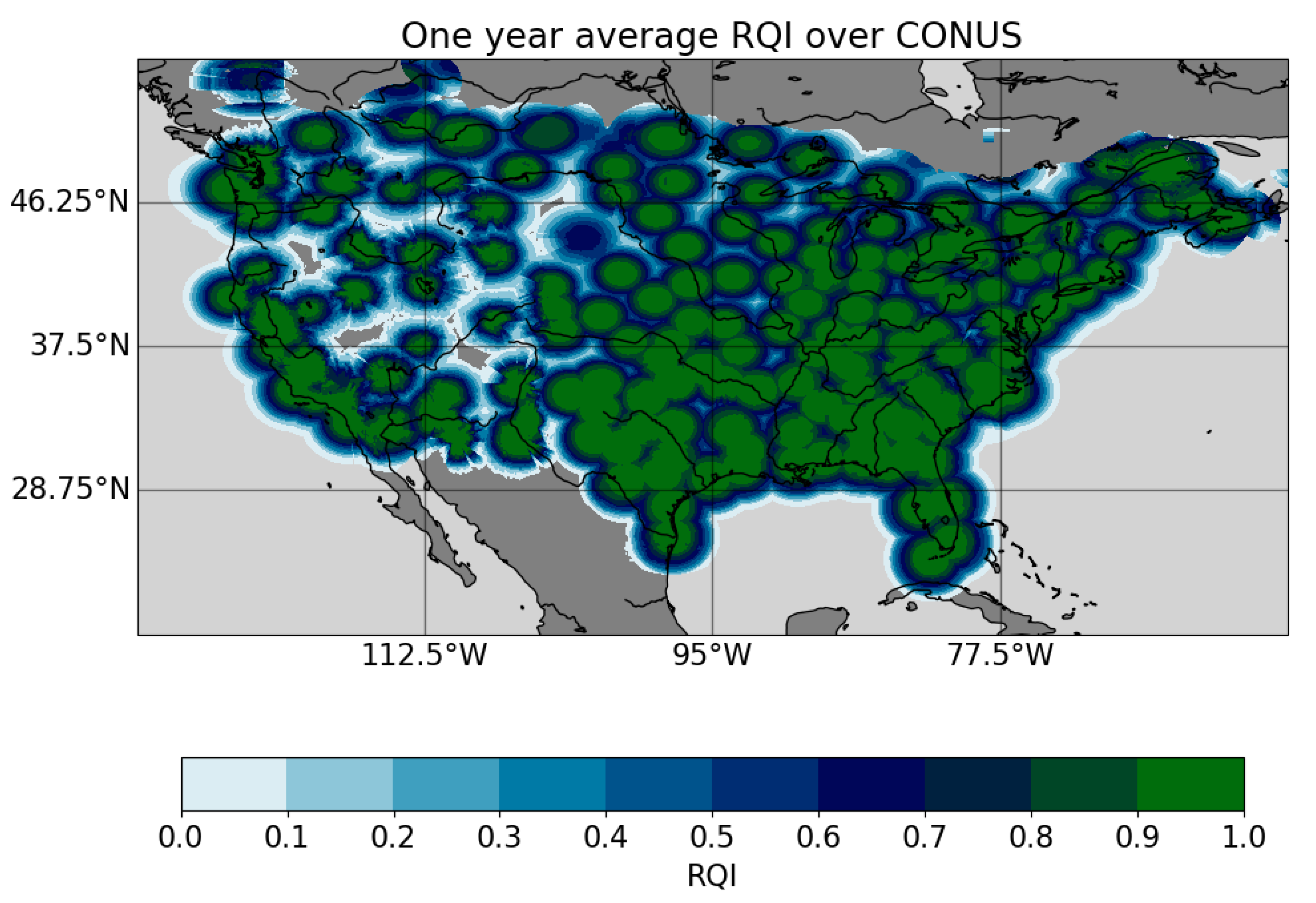
2.5.1. Regional Verification Methodology

For the regional verification over the CONUS area the L2 instantaneous precipitation rate data from PNPR-CLIM, GPROF and MRMS were used. The inter-comparisons between the PNPR-CLIM and GPROF instantaneous retrievals and the MRMS radar-only instantaneous precipitation product, were carried out considering all the MHS observations, from 2015 to 2017, within the CONUS area. Following [77], for each MHS observation pixel, the nearest MRMS grid point was identified and the radar precipitation product was averaged to a coarser resolution of 15 km × 15 km. In addition, to filter out unreliable radar data, a one-year set of MRMS observations was used to produce a daily, 15 km resolution, average quality index which was applied to select high-quality observations. All the observations with daily quality index lower than 0.9 were discarded from the analysis. The hypothetical geographical coverage of the selected observations is given in Figure 1, where the one-year average MRMS radar quality index is shown. Furthermore, the validation was carried out only for liquid precipitation, discarding all observations where GPROF indicated frozen precipitation rate > 0 mm/h.

2.5.2. Global Verification Methodology

For the inter-comparison on a global scale two analyses were performed. Firstly, an entire one-year (2016) set of observations was selected from the DPR-MHS coincidence dataset for validation. The algorithm was evaluated focusing on two distinct aspects: instantaneous precipitation detection and estimate. Secondly, to evaluate the algorithm against independent datasets, a three-year (2015–2017) analysis of PNPR-CLIM, GPROF and GPCP was carried out. PNPR-CLIM and GPROF datasets were processed to make them comparable to GPCP, that is, 1° × 1° spatial resolution and at daily temporal resolution. The PNPR-CLIM and GPROF L2 precipitation rates were spatially aggregated (by averaging over all the MHS pixels within each grid box) to produce a gridded global hourly product. This intermediate dataset was further aggregated over 24 h to obtain a daily product.

Passive MW radiometers are carried out by LEO satellites and have a repetition time of several hours. Therefore, estimating the daily precipitation from them is not trivial. For the present study, 4 satellites were considered: NOAA-18/19 and MetOp-A/B, whose ascending equatorial crossing times are shown in Figure 2. Since the two MetOp satellites have equal ascending nodes, only 6 independent observations were guaranteed within each day. The undersampling problem was tackled in previous works, over limited areas (e.g., [78]) and for some case studies, (e.g., [79,80]) tested the possibility of monitoring intense precipitating events using PMW observations only. Their results show a strong dependence on the number of available overpasses and their temporal distribution. In this context the comparison between PNPR-CLIM or GPROF with GPCP is biased by the number of daily overpasses at a given latitude and by their spread within the day, that will affect the representativeness of the precipitation daily cycle. Nevertheless, the two sets of PMW-derived daily precipitations were obtained by considering the same collection of observations, namely the MHS measurements taken onboard NOAA-18/19 and MetOp-A/B, and therefore the error contribution due to the sparse sampling is the same in both the datasets. In this perspective, the comparison with GPCP has the only scope to assess the impact of the existing differences between the two retrieval algorithms on a global scale, as the actual estimations can not be adjusted to recover the higher frequency (i.e., sub-daily) processes associated with the precipitation.

2.6. Statistical Scores

A brief summary of the statistical scores used in the study for the verification at regional and global scale is provided, while for detailed definitions the reader is referred to [81].

For the precipitation/no-precipitation categorization the following indices are exploited—the Probability of detection (POD), False alarm rate (FAR), accuracy (ACC) and Heideke skill score (HSS). POD is the fraction of positive events correctly classified, FAR is the fraction of false positive events arisen by the model, ACC is the fraction of correctly classified events and HSS measures the model improvement with respect to the random classifier (HSS = 0 means no improvements, HSS = 1 means perfect score).

The following metrics are introduced for quantitative verification—the mean error (ME), root mean squared error (RMSE), and linear correlation coefficient. (CC). The ME and RMSE metrics measure the model departure from the reference, whereas the CC measures the covariance degree between the two.

3. Algorithm Description

3.1. The MHS-DPR Coincidence Dataset

The dataset used for the development of PNPR-CLIM consisted of two years (2015–2016) of coincident observations (within a time interval of 15 min) between MHS swath, on-board NOAA-18, NOAA-19, MetOp-A and MetOp-B, and the GPM-CO DPR swath. The surface precipitation rate from the GPM 2B-CMB product (version 06A), which combines DPR and GPM Microwave Imager (GMI) measurements, was used as reference [82,83]. The precipitation rate estimates provided by the DPR Normal Scan (NS) (Ku-band radar) swath (245 km wide) was used.

The training dataset is made of co-located vectors of FIDUCEO FCDR AMSU-B/MHS BTs and ancillary variables Table 2, and 2B-CMB (hereafter referred to as DPR) surface precipitation rates spatially averaged to match the sensor instantaneous field of view (IFOV), variable along the scan (see also [35]).

Table 4. Characteristics of the AMSU-B/MHS-DPR coincidence dataset.

Period	1 January 2015/31 December 2016
Geographical area	65° S–65° N/180° W–180° E
Num. of pixels	48 × ${10}^6$
Num. of prec. pixels	6.8 × ${10}^6$
Reference product	DPR-GMI 2B-CMB v06A (swath NS)
AMSU-B/MHS BTs	FIDUCEO FCDR v4.1

summarizes the dataset characteristics.

The entire dataset was divided into two parts—the 2015 dataset was used to train the algorithm, and 2016 dataset was used for validation. In addition, the first dataset was further randomly divided into two parts: 80% used for training and 20% used to monitor (and prevent) over-fitting during the optimization phase.

PNPR-CLIM Design

The PNPR-CLIM algorithm consists of two distinct NN-based modules, the precipitation classification module (PCM) and the precipitation estimate module (PEM), conceived by benefiting from the experience gained during the development of previous versions of PNPR algorithm for cross-track scanning MW radiometers (PNPR v1 for AMSU/MHS and PNPR v2 for ATMS, described in [35,36]). The PCM is designed to estimate the pixel-based probability of precipitation conditioned to the input vector state (AMSU-B and MHS BTs and ancillary variables). It is composed of a single NN with three hidden layers of 45, 15 and 1 neurons respectively, connected by sigmoid transfer functions. Its output is a continuous function with values in the range [0,1] which, under suitable hypotheses on the training dataset distribution [84], approximates the precipitation probability conditioned to the input state. The threshold value of 0.5 is used to distinguish precipitating (above 0.5) and non-precipitating states (below 0.5, inclusive). The PEM evaluates the pixel-based instantaneous precipitation rate for observations classified as precipitating by the PCM. Also the PEM consists of a single NN with three hidden layers of 28, 8 and 1 neurons respectively, connected by sigmoid transfer functions.

Model selection in NNs aims at finding as few hidden layers and neurons as necessary for a good approximation of the true function. Thus, two relatively distinct aspects must be considered—determining how many layers to use and how many neurons to include in each layer. In the present work the model selection was carried out using a cross-validation method [35,85,86]. Several different combinations of layers, neurons per layer and transfer functions were therefore tested. The resulting architecture proved to be the most adaptive and performing.

It is worth noting that the use of different NNs for different types of surfaces [33] is suggested by the remarkably different characteristics of the microwave signatures on different backgrounds, especially in the window channels (e.g., 89 GHz) and/or in dry atmospheric conditions. However, the use of different NNs can often lead to discontinuity of the estimates in correspondence with background surface transitions. The single-NN approach prevents this kind of discontinuities or inconsistencies in the retrieved precipitation patterns, while making the various phases of the design more complex (training, learning, network architecture, and selection of inputs).

4. Results and Discussion

4.1. Global Verification with DPR

The PCM and PEM performances were tested using the 2016 MHS-DPR coincidence dataset, which is an independent part of the full observational MHS-DPR coincidence dataset (Section 3.1), not used in the training and design phase of the algorithm.

4.1.1. PCM Performances

To assess the PCM performance, the ACC, HSS, POD and FAR scores were computed as a function of the detection threshold $\delta$, meaning that DPR estimates above (below) $\delta$ denoted precipitating (non-precipitating) conditions. Notice that the variations of $\delta$ do not change the proportion of the predicted positives/negatives, thus, to balance the effect of introducing fictitious false alarms by increasing $\delta$ (small rates correctly identified as non-zero), the various indices were computed on the reduced population given by those pixels with DPR rate either equal to 0 mm/h or greater than $\delta$. The results are shown in Figure 3. In the figure, the ACC values are quite stable, around 0.94 above 0.1 mm/h. The HSS maximum (0.71) is achieved at about 0.32 mm/h. At the same threshold, POD is 0.80 and FAR is 0.33. The POD increases beyond 0.86 above 0.5 mm/h. The FAR value at the 0 mm/h threshold is 0.21. In the light of these results, the minimum threshold of 0.32 mm/h (HSS maximum location) can be assumed as the PNPR-CLIM sensitivity limit.

It should be highlighted that, despite PNPR-CLIM was trained to reproduce the DPR product, the perfect agreement is not achieved. However, this is expected for several reasons. Firstly, the GMI and DPR instruments, fully exploited in the 2B-CMB product, have peculiar characteristics (sensitivity, spatial resolution) and enhanced precipitation sensing capabilities compared to MHS. Secondly, the coincidences are affected by spatio-temporal uncertainties, due to their different scan geometries and orbits. Nevertheless, the present results are in-line with those obtained in [37], where a precipitation retrieval algorithm designed for the conically scanning GMI radiometer is trained and tested against the same DPR product.

4.1.2. PEM Performances

In the PEM performance analysis, the precipitation distribution of the NN was compared with the reference (DPR). Only pixels where both PEM and DPR provide rainfall rate ≥0.1 mm/h (hits) were considered in order to evaluate the agreement between the PEM and the DPR estimates in presence of relevant precipitation. The 0.1 mm/h threshold was chosen as a compromise between the DPR detection threshold (0.2 mm/h in the Ka band and 0.5 mm/h in the Ku band) and the smoothing resulting from the averaging procedure. Figure 4 shows the density scatterplot of the surface rain rate estimates (mm/h) from the PEM and the corresponding values of DPR in the verification dataset, over ocean and land. The figure shows a very good consistency between the two products, with a quite homogeneous trend in the two panels. Most of the points are close to the main diagonal for both ocean and land, with a slight overestimation by PEM for low precipitation rain rate <0.5 mm/h over land. It should be noted that these discrepancies appear at low regimes, when the scattering signal within the upwelling radiation can easily fall below the radiometer sensitivity. The accuracy statistical scores (ME, RMSE and CC) obtained for PEM (hits only), were ME = 0.10 mm/h, RMSE = 1.09 mm/h and CC = 0.71 over ocean, and ME = 0.11 mm/h, RMSE = 1.10 mm/h and CC = 0.70 over land.

4.2. Regional Verification over CONUS

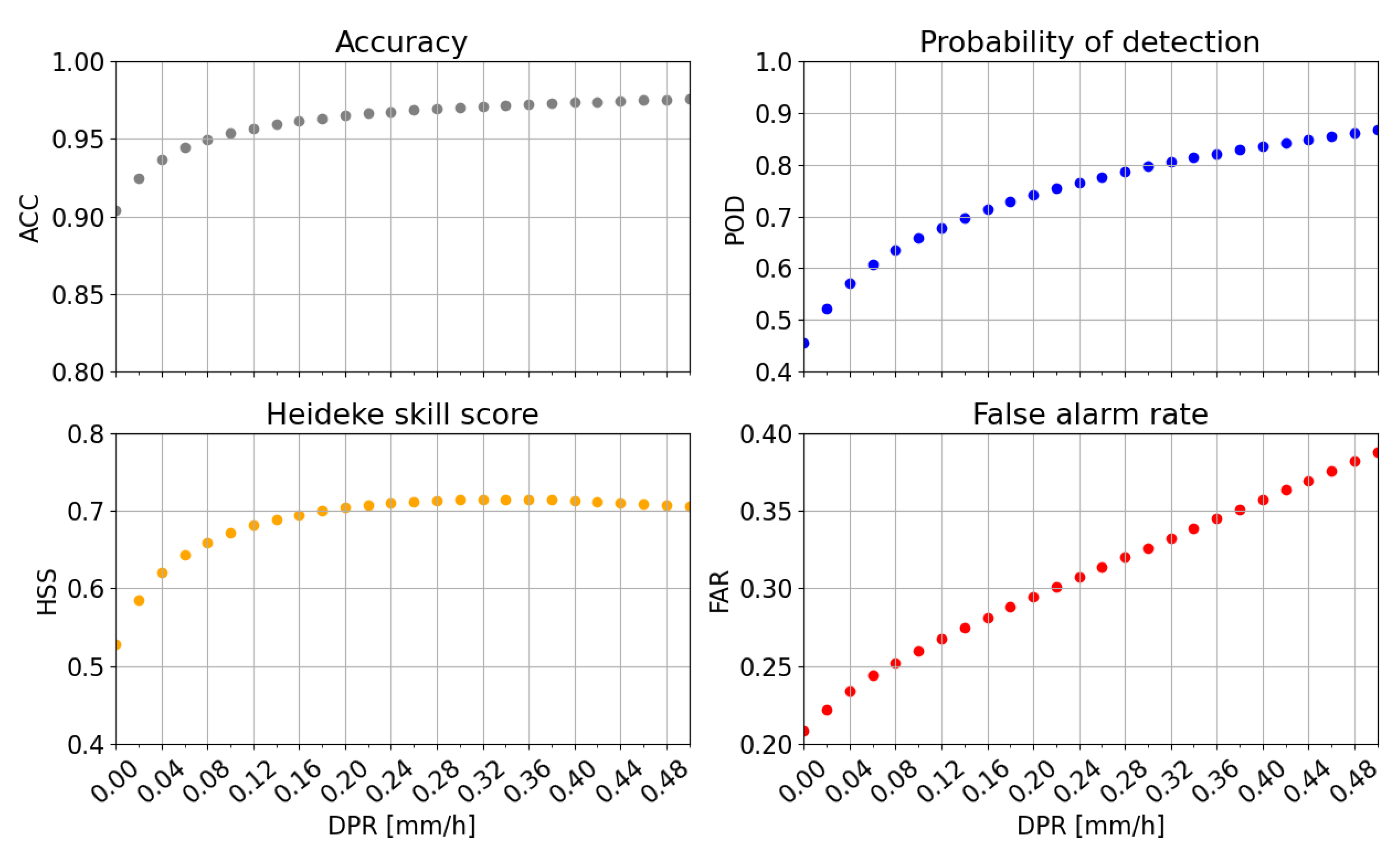
4.2.1. Precipitation Detection

The first analysis over CONUS involved the detection statistics. It should be highlighted that, ground-based radar data and satellite observations, besides the resolution heterogeneity and sampling asynchrony, have different sensitivity thresholds (for MRMS it corresponds to the minimum 5 dBz reflectivity threshold, [68]). For these reasons, all the precipitation events correctly identified by the radar but likely missed by the satellite sensor should be removed before the assessment. Indeed, events with either low intensity (below the radiometer sensitivity threshold) or small spatial extension (a little fraction of the sensor resolution) do not contribute to the algorithm evaluation. In this verification each regridded MRMS pixel (15 km resolution) was classified as precipitating if its average precipitation rate is greater than 0.1 mm/h and the area covered by precipitation within it, with respect to the native grid (at 0.01° resolution), is greater than 90%, whereas in the non-precipitating portion the average precipitation rate was zero. With this convention, 2.2% of the entire population was classified as precipitating.

HSS, POD and FAR (see Section 2.6) were computed at different values of the detection threshold $\delta$, as reported in Figure 5. Note that this analysis was different from that carried out for the verification of PCM described in Section 4.1.1 as, in this case, the threshold is applied to the predictions too. In the figure, the indices show that PNPR-CLIM generally achieves better results than GPROF, especially for low detection thresholds, both in terms of single classes predictions (POD and FAR) and aggregated ones (HSS). The differences are quite evident especially in terms of FAR, for small detection thresholds ($\delta \le$ 0.2 mm/h), with PNPR-CLIM showing significantly lower values than GPROF. At $\delta$ = 0.3 mm/h the the FAR for two products tend to converge (around 0.35), while PNPR-CLIM has consistently higher POD (0.80) and HSS (above 0.70) than GPROF.

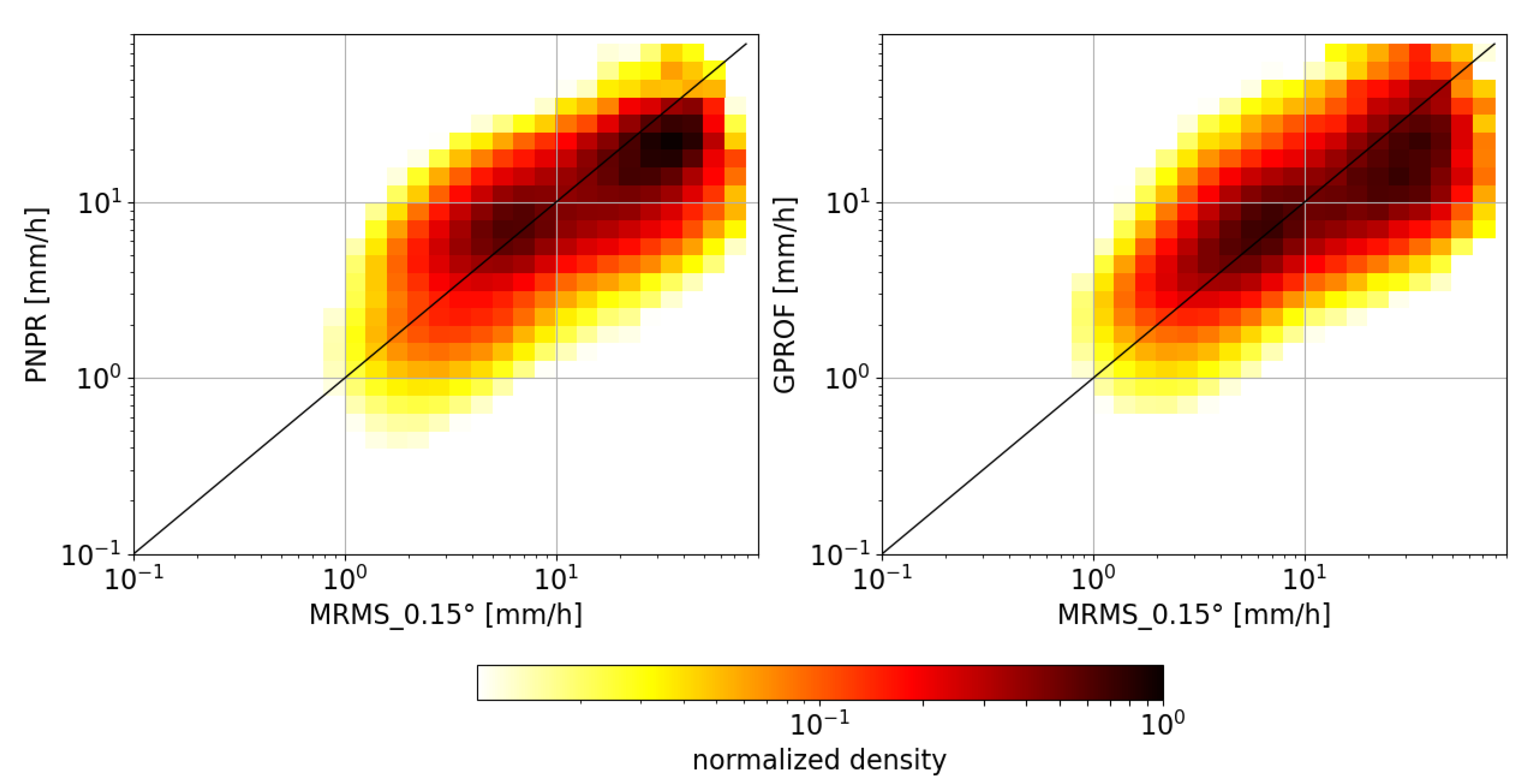
4.2.2. Precipitation Estimate

The second evaluation concerned the comparisons of the precipitation distributions of the three products, PNPR-CLIM, GPROF, and MRMS.

In Figure 6 the joint normalized densities between products and reference are displayed (from left to right: PNPR-CLIM with MRMS and GPROF with MRMS). In the panels, the color of each gridbox $[x_1,x_2]\times [y_1,y_2]$ corresponds to the number of observations for which the reference (on the x-axis) and the product (on the y-axis) have values in $[x_1,x_2)$ and $[y_1,y_2)$ respectively, finally weighted by the bin area $(x_2-x_1)(y_2-y_1)$. Note that the two densities were additionally normalized (by a common factor) to have non-dimensional units between 0 and 1. In

Table 5. ME, RMSE and CC between PNPR-CLIM, GPROF and MRMS using the entire dataset.

	ME (mm/h)	RMSE (mm/h)	CC
PNPR-CLIM vs. MRMS	−0.007	0.606	0.712
GPROF vs. MRMS	0.005	0.621	0.712
PNPR-CLIM vs. GPROF	−0.012	0.393	0.853

, the values of the three metrics ME, RMSE and CC (computed including zeros) are also reported. Both the satellite products tend to underestimate heavy precipitation regimes (>10 mm/h), although GPROF spreads these rates on a wider range, as the smoothness of the rightmost peak testifies. In the same range, the GPROF underestimations are more severe than those of PNPR-CLIM, peaking at about 30 mm/h (referred to MRMS). For moderate rates (<10 mm/h), both PNPR-CLIM and GPROF overestimate MRMS with no notable differences. At about 3 mm/h, PNPR-CLIM shows a weak underestimate, towards 1 mm/h, of MRMS. The same tendency is experienced by GPROF, although less perceptible. The ME value is negative for PNPR-CLIM (−0.007 mm/h), and positive for GPROF (0.005 mm/h). This anomaly is likely due to the occasional high rates overestimates of GPROF. The lower RMSE value achieved by PNPR-CLIM (0.606 mm/h, compared to 0.621 mm/h by GPROF) confirms this observation Table 5. Finally, the CC value, which for both products is 0.712, proves the good consistency of the two algorithms, as their relative low RMSE (0.393 mm/h) and high CC (0.853) testify.

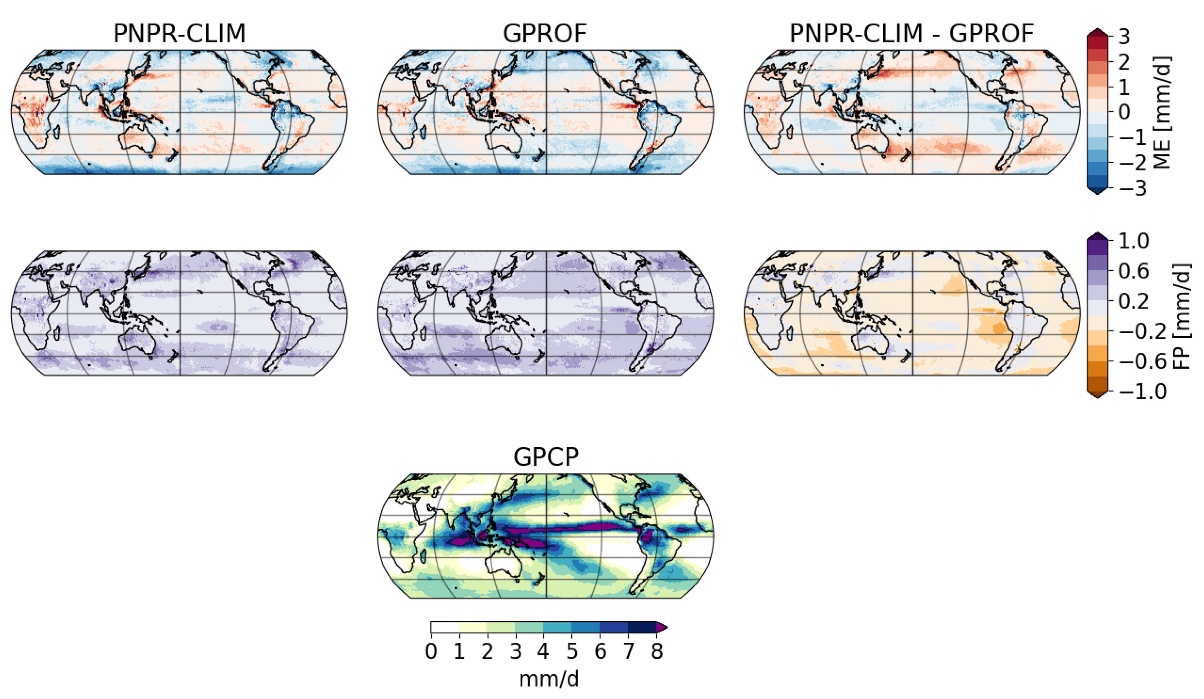
4.3. Global Comparison of PNPR-CLIM and GPROF with GPCP

4.3.1. Mean Errors

The first part of the global verification and intercomparison involved the evaluation of the ME and False Precipitation (FP) global maps (over a 1° × 1° regular grid) of PNPR-CLIM and GPROF precipitation fields against the GPCP dataset for the period 2015–2017. The results are shown in Figure 7, where the ME was computed in each grid box with respect to the time dimension onlys (first row). In the same figure FP represents the mean daily false precipitation of PNRP-CLIM and GPROF referred to GPCP (second row), that is, the average non-zero daily precipitation relative to the non-rainy days [3]. The ME and FP differences between PNPR-CLIM and GPROF are also shown (right panels).

The PNPR-CLIM errors show higher ME values over different regions—southern Pacific, southeastern Asia and central Africa. Smaller areas, off the coast of Japan and Eastern US, in the northwestern Atlantic and northwestern Pacific respectively, are also characterized by locally larger values. In contrast, in GPROF these anomalies are either less pronounced (over land) or reversed (over ocean), as highlighted in the upper right panel showing the ME differences. It is worth noting that these regions are characterized by high annual precipitation values (as shown by the GPCP mean values). So, the PNPR-CLIM overestimations could be related to the scarce sampling, which forces the daily mean rate to be aligned with the only available observations of intense precipitation (see Section 2.5.2). The same regions are also affected by moderate values of FP, indicating the existence of non-zero estimated precipitation during non-rainy days. However, these areas are well localized.

Looking at the GPROF maps, instead, it emerges that the ocean areas where GPROF exhibits greater ME values (i.e., central Pacific and Indian oceans, as shown in the upper right panel of Figure 7) coincide with regions manifestly characterized by high FP levels. Notice that FP represents the amount of estimated precipitation in non-rainy days and, as such, it turns out to be independent of the sampling scheme (i.e., increasing the number of observations does not make the field vanish). This suggests that GPROF actually retrieves more precipitation than the reference over these wide ocean areas. It is generally true that, over ocean, GPROF FPs are higher, while, over land, PNPR-CLIM shows moderately higher values although GPROF exhibits greater peaks (e.g., southern Brasil).

4.3.2. CC and RMSE

In the second part of the analysis, the RMSE and CC global maps referred to GPCP were considered; the results are shown in Figure 8. As already explained, the absolute values of the RMSE (as well as of the ME) are of moderate interest due to the inherent undersampling errors. In this analysis, the main focus is on the differences between the results obtained for GPROF and PNPR-CLIM when compared to the same reference (GPCP), rather than their actual performances against GPCP. The CC metric, instead, is a more effective parameter to consider for the assessment, also for the comparison with GPCP per se, as it provides a measure of the temporal coherence between the various products regardless of their actual mean values.

It is evident that PNPR-CLIM shows a better agreement with GPCP than GPROF over ocean, as the relative lower RMSE and the higher CC highlight; although the RMSE values are everywhere higher than the GPCP mean. In particular, GPROF exhibits higher values of RMSE almost everywhere, both on ocean and land. As expected, the higher values are visible in the wet regions (see Figure 8, bottom panel)—central Pacific and northern Atlantic, southeastern Asia, central Africa, southern and central America. The CC field shows analogous patterns. PNPR-CLIM has higher CC over the ocean: above 0.4 at high latitudes and between 0.5 and 0.8 at mid and low latitudes, increasing towards the Equator. Also GPROF shows the same CC spatial patterns, although with smaller values. GPROF performance is moderately better than that of PNPR-CLIM over land: both the products do not exceed the value of 0.7 and are frequently between 0.4 and 0.5.

4.4. Zonal Means

Figure 9 shows the comparisons of the zonal means of PNPR-CLIM, GPROF and GPCP over the considered period (2015–2017). The averaging was performed by categorizing per surface type (global, ocean, and land) and per season.

Despite the limitations due to the passive microwave products’ sampling scheme, the overall zonal means of the satellite products considerably agree with the GPCP estimates, particularly in the 30° N/S latitude range. The major difference is observed over land at about 10° S during the wet seasons in DJF and MAM. Notable divergences between the products were already observed in central America and central Africa at this latitude (Section 4.3.1), which now reflect on the zonal means. However, PNPR-CLIM and GPROF respond differently in these zones, indicating a substantial difference of the two algorithms in estimating the peculiar precipitation of these areas.

The agreement between PNPR-CLIM and GPCP is still appreciable up to 40° N/S, whereas the GPROF estimations result in a sensible lack of precipitation around 40° N/S due to the underestimation over the ocean. At higher latitudes also PNPR-CLIM underestimates GPCP with a more pronounced effect during the winter season. This is a typical limitation of the DPR-based precipitation products, that fail to accurately depict the high latitudes precipitation and snowfall, as recently pointed out by several studies (e.g., [46,87]).

5. Conclusions

The new PNPR-CLIM algorithm was designed and developed using an NN approach within the Copernicus C3S project to produce a long-term global L2 precipitation rate dataset based on the AMSU-B and MHS measurements. The algorithm was successfully trained with a one-year (2015) observational dataset composed of coincident calibrated BTs of the radiometers (provided by FIDUCEO FCDR records) and the GPM GMI-DPR precipitation estimates used as reference. The algorithm has shown remarkable adaptive properties, as demonstrated in the global verification analysis carried out with an independent set of DPR-based precipitation data. The estimated precipitation distribution over one year (2016) turned out to be in good agreement with the DPR estimates, testifying the successful parametrization of the precipitation radiative properties achieved by the NNs. In addition, the use of a single NN has responded correctly at transitions among different surface backgrounds, without introducing discontinuities in the precipitation distributions.

Since the DPR-based product was used as reference during the training, the algorithm was additionally tested against other independent precipitation products on a regional scale. The analysis was carried out over the CONUS area, considering instantaneous precipitation rates obtained from the GPROF algorithm (applied to the AMSU-B/MHS BTs) and MRMS over a period of three year (2015–2017). For the comparison, all the three datasets were adjusted to a common resolution of 15 km × 15 km. In addition, the radar quality information was used to select the most reliable data only. The assessment confirmed the positive performance of PNPR-CLIM highlighted during the verification against DPR. Moreover, the dichotomous statistical scores proved to be better than those of GPROF—for a detection threshold of 0.3 mm/h, PNPR-CLIM showed an HSS of 0.73, a POD of 0.81 and a FAR of 0.33, while GPROF achieved an HSS of 0.69, a POD of 0.77 and a FAR equal to 0.36. Regarding the verification on the estimates against MRMS, the two algorithms’ performances were quite similar—PNPR-CLIM showed ME, RMSE and CC of about −0.007 mm/h, 0.606 mm/h and 0.712, respectively, while for GPROF the scores were 0.005 mm/h, 0.621 mm/h and 0.712, respectively. No appreciable differences were observed, but a less pronounced underestimation of the MRMS high rates by PNPR-CLIM than GPROF (above 10 mm/h, as inferred from Figure 5).

Then, the global verification, covering the three-year period 2015–2017, was carried out by comparing PNPR-CLIM and GPROF with the GPCP 1DD v1.3 product (at daily time scale and over a 1° × 1° regular grid). Considering the inherent limitation of such analysis, mainly related to the low-frequency temporal sampling of the daily precipitation by the passive microwave products, notable differences between GPROF and PNPR-CLIM were highlighted. The analysis has showed that the GPROF performances over land were slightly better than those of PNPR-CLIM, although both the products showed large underestimates over tropical regions, like central America and southeastern Asia. These regions are characterized by strong Monsoon activities, and it is likely that the few satellite overpasses strongly constrain the local estimates, as the daily cycles are not properly resolved. Differently, in central Africa, both PNPR-CLIM and GPROF overestimated the precipitation compared to GPCP.

However, to understand the source of these differences, further local analyses should be carried out, using high-frequency ground based measurements if available. Indeed, these environments have unique characteristics—the great amount of total precipitable water in the Amazon during the wet season, for instance, produces very peculiar atmospheric profiles, potentially masking the precipitation-related upwelling signal (in the available AMSU-B and MHS frequency channels) from the lower troposphere. Over ocean, instead, the PNPR-CLIM performances turned out to be moderately better than those of GPROF: the overall CC was higher and the RMSE was lower.

The comparison of the zonal means confirmed these remarks and additionally highlighted the quick GPROF performance degradation above 40° N/S, contrarily to PNPR-CLIM, which was still very similar to GPCP. At higher latitudes, however, both PNPR-CLIM and GPROF showed to miss relevant amounts of precipitation.

In summary, the algorithm proved to be very effective in retrieving the precipitation using a combination of MHS/AMSU-B observations and model derived variables. Nevertheless, the global verification at daily scale showed complex error features across the globe, not exclusively related to the undersampling associated with the satellites overpasses frequency, as evidenced by some spatial error features. Especially over complex surface backgrounds (e.g., tropical rainforest) high errors were observed. Indeed, peculiar environments could be marginally described in a global training dataset, which is the only source of information of the NNs. More precisely, the representativeness of typical high variable regimes of small areas, like the Amazon, was not guaranteed in the training dataset, although it counted more than 20 million pixels of MHS-DPR coincidences collected over one year. In fact, a few hundreds of observations taken over one wet season can not be representative of the complex and peculiar dynamics characterizing such regions and, moreover, turn out to be statistically rare within the training dataset and thus easily ignored during the NN optimization phase. Together with the lack of microwave observations below 89 GHz, essential for the background surface characterization, this explains the variable performances of the algorithm across the globe, especially at high latitudes. In this regard, one of the challenges for satellite precipitation retrieval is the improvement of high latitude precipitation estimation (light rain/drizzle and snowfall) [87,88,89]. CloudSat-based machine learning snowfall retrieval techniques seem to be very promising to this purpose [66,90,91,92]. Specific efforts will be dedicated in the future to the improvement of snowfall detection and estimation in PNPR-CLIM. In particular, an analysis will be carried out aimed at detecting snowfall and retrieve the associated snow rate through the development of dedicated modules. Also these modules will be based on machine learning techniques and will be applied to a training dataset based on AMSU-B and MHS coincident observations with the Cloud Profiling Radar onboard CloudSat.

References

1. Ebert, E.E.; Janowiak, J.E.; Kidd, C. Comparison of near-real-time precipitation estimates from satellite observations and numerical models. Bull. Am. Meteorol. Soc. 2007, 88, 47–64. [Google Scholar] [CrossRef] [Green Version]
2. Lin, X.; Hou, A.Y. Evaluation of coincident passive microwave rainfall estimates using TRMM PR and ground measurements as references. J. Appl. Meteorol. Climatol. 2008, 47, 3170–3187. [Google Scholar] [CrossRef]
3. Tian, Y.; Peters-Lidard, C.D.; Eylander, J.B.; Joyce, R.J.; Huffman, G.J.; Adler, R.F.; Hsu, K.l.; Turk, F.J.; Garcia, M.; Zeng, J. Component analysis of errors in satellite-based precipitation estimates. J. Geophys. Res. Atmos. 2009, 114. [Google Scholar] [CrossRef] [Green Version]
4. Iturbide-Sanchez, F.; Boukabara, S.A.; Chen, R.; Garrett, K.; Grassotti, C.; Chen, W.; Weng, F. Assessment of a variational inversion system for rainfall rate over land and water surfaces. IEEE Trans. Geosci. Remote Sens. 2011, 49, 3311–3333. [Google Scholar] [CrossRef]
5. Brocca, L.; Ciabatta, L.; Massari, C.; Moramarco, T.; Hahn, S.; Hasenauer, S.; Kidd, R.; Dorigo, W.; Wagner, W.; Levizzani, V. Soil as a natural rain gauge: Estimating global rainfall from satellite soil moisture data. J. Geophys. Res. 2014, 119, 5128–5141. [Google Scholar] [CrossRef]
6. Kidd, C.; Matsui, T.; Chern, J.; Mohr, K.; Kummerow, C.; Randel, D. Global precipitation estimates from cross-track passive microwave observations using a physically based retrieval scheme. J. Hydrometeorol. 2016, 17, 383–400. [Google Scholar] [CrossRef] [Green Version]
7. Beck, H.E.; Wood, E.F.; Pan, M.; Fisher, C.K.; Miralles, D.G.; Van Dijk, A.I.; McVicar, T.R.; Adler, R.F. MSWep v2 Global 3-hourly 0.1° precipitation: Methodology and quantitative assessment. Bull. Am. Meteorol. Soc. 2019, 100, 473–500. [Google Scholar] [CrossRef] [Green Version]
8. Levizzani, V.; Cattani, E. Satellite Remote Sensing of Precipitation and the Terrestrial Water Cycle in a Changing Climate. Remote Sens. 2019, 11, 2301. [Google Scholar] [CrossRef] [Green Version]
9. Gao, Z.; Huang, B.; Ma, Z.; Chen, X.; Liu, D.; Qiu, J. Comprehensive comparisons of state-of-the-art gridded precipitation estimates for hydrological applications over southern China. Remote Sens. 2020, 12, 3997. [Google Scholar] [CrossRef]
10. Kidd, C.; Huffman, G. Global precipitation measurement. Meteorol. Appl. 2011, 18, 334–353. [Google Scholar] [CrossRef]
11. Kucera, P.A.; Lapeta, B. Leading Efforts to Improve Global Quantitative Precipitation Estimation. Bull. Am. Meteorol. Soc. 2014, 95, 26–29. [Google Scholar] [CrossRef]
12. Wilheit, T. Algorithms for the retrieval of rainfall from passive microwave measurements. Remote Sens. Rev. 1994, 11, 163–194. [Google Scholar] [CrossRef]
13. Weng, F.; Grody, N.C. Retrieval of ice cloud parameters using a microwave imaging radiometer. J. Atmos. Sci. 2000, 57, 1069–1081. [Google Scholar] [CrossRef]
14. Bennartz, R.; Petty, G.W. The sensitivity of microwave remote sensing observations of precipitation to ice particle size distributions. J. Appl. Meteorol. 2001, 40, 345–364. [Google Scholar] [CrossRef]
15. Bauer, P.; Moreau, E.; Di Michele, S. Hydrometeor retrieval accuracy using microwave window and sounding channel observations. J. Appl. Meteorol. 2005, 44, 1016–1032. [Google Scholar] [CrossRef]
16. Kidd, C.; Matsui, T.; Ringerud, S. Precipitation Retrievals from Passive Microwave Cross-Track Sensors: The Precipitation Retrieval and Profiling Scheme. Remote Sens. 2021, 13, 947. [Google Scholar] [CrossRef]
17. Wang, J.R.; Zhan, J.; Racette, P. Storm-Associated Microwave Radiometric Signatures in the Frequency Range of 90–220 GHz. J. Atmos. Ocean. Technol. 1997, 14, 13–31. [Google Scholar] [CrossRef]
18. Staelin, D.H.; Chen, F.W. Precipitation observations near 54 and 183 GHz using the NOAA-15 satellite. IEEE Trans. Geosci. Remote Sens. 2000, 38, 2322–2332. [Google Scholar] [CrossRef] [Green Version]
19. Blackwell, W.; Chen, F. Neural Network Applications in High-Resolution Atmospheric Remote Sensing. Licoln Lab. J. 2005, 15, 299–322. [Google Scholar]
20. Burns, B.A. Effects of precipitation and cloud ice on brightness temperatures in AMSU moisture channels. IEEE Trans. Geosci. Remote Sens. 1997, 35, 1429–1437. [Google Scholar] [CrossRef]
21. Ferraro, R.R.; Weng, F.; Grody, N.C.; Zhao, L.; Meng, H.; Kongoli, C.; Pellegrino, P.; Qiu, S.; Dean, C. NOAA operational hydrological products derived from the advanced microwave sounding unit. IEEE Trans. Geosci. Remote Sens. 2005, 43, 1036–1049. [Google Scholar] [CrossRef]
22. Hong, G.; Heygster, G.; Miao, J.; Kunzi, K. Detection of tropical deep convective clouds from AMSU-B water vapor channels measurements. J. Geophys. Res. D Atmos. 2005, 110. [Google Scholar] [CrossRef] [Green Version]
23. Hong, G.; Heygster, G.; Notholt, J.; Buehler, S.A. Interannual to diurnal variations in tropical and subtropical deep convective clouds and convective overshooting from seven years of AMSU-B measurements. J. Clim. 2008, 21, 4168–4189. [Google Scholar] [CrossRef]
24. Funatsu, B.M.; Claud, C.; Chaboureau, J.P. Potential of Advanced Microwave Sounding Unit to identify precipitating systems and associated upper-level features in the Mediterranean region: Case studies. J. Geophys. Res. Atmos. 2007, 112. [Google Scholar] [CrossRef]
25. Funatsu, B.M.; Claud, C.; Chaboureau, J.P. Comparison between the large-scale environments of moderate and intense precipitating systems in the Mediterranean region. Mon. Weather Rev. 2009, 137, 3933–3959. [Google Scholar] [CrossRef] [Green Version]
26. Laviola, S.; Levizzani, V. The 183-WSL fast rain rate retrieval algorithm. Part I: Retrieval design. Atmos. Res. 2011, 99, 443–461. [Google Scholar] [CrossRef]
27. Ferraro, R. The Status of the NOAA/NESDIS Operational AMSU Precipitation Algorithm. In Proceedings of the 2nd Workshop of the International Precipitation Working Group, Monterey, CA, USA, 25–28 October 2004; p. 9. [Google Scholar]
28. Qiu, S.; Pellegrino, P.; Ferraro, R.; Zhao, L. The improved AMSU rain-rate algorithm and its evaluation for a cool season event in the western United States. Weather Forecast. 2005, 20, 761–774. [Google Scholar] [CrossRef]
29. Liou, Y.-A.; Tzeng, Y.C.; Chen, K.S. A neural-network approach to radiometric sensing of land-surface parameters. IEEE Trans. Geosci. Remote Sens. 1999, 37, 2718–2724. [Google Scholar] [CrossRef]
30. Aires, F.; Prigent, C.; Rossow, W.B.; Rothstein, M. A new neural network approach including first guess for retrieval of atmospheric water vapor, cloud liquid water path, surface temperature, and emissivities over land from satellite microwave observations. J. Geophys. Res. Atmos. 2001, 106, 14887–17907. [Google Scholar] [CrossRef]
31. Ashouri, H.; Hsu, K.L.; Sorooshian, S.; Braithwaite, D.K.; Knapp, K.R.; Cecil, L.D.; Nelson, B.R.; Prat, O.P. PERSIANN-CDR: Daily Precipitation Climate Data Record from Multisatellite Observations for Hydrological and Climate Studies. Bull. Am. Meteorol. Soc. 2015, 96, 69–83. [Google Scholar] [CrossRef] [Green Version]
32. Hong, Y.; Hsu, K.L.; Sorooshian, S.; Gao, X. Precipitation estimation from remotely sensed imagery using an artificial neural network cloud classification system. J. Appl. Meteorol. 2004, 43, 1834–1853. [Google Scholar] [CrossRef] [Green Version]
33. Surussavadee, C.; Staelin, D. Global Millimeter-Wave Precipitation Retrievals Trained with a Cloud-Resolving Numerical Weather Prediction Model, Part I: Retrieval Design. IEEE Trans. Geosci. Remote Sens. 2008, 46, 99–108. [Google Scholar] [CrossRef]
34. Mahesh, C.; Prakash, S.; Sathiyamoorthy, V.; Gairola, R.M. Artificial neural network based microwave precipitation estimation using scattering index and polarization corrected temperature. Atmos. Res. 2011, 102, 358–364. [Google Scholar] [CrossRef]
35. Sanò, P.; Panegrossi, G.; Casella, D.; Di Paola, F.; Milani, L.; Mugnai, A.; Petracca, M.; Dietrich, S. The Passive microwave Neural network Precipitation Retrieval (PNPR) algorithm for AMSU/MHS observations: Description and application to European case studies. Atmos. Meas. Tech. 2015, 8, 837–857. [Google Scholar] [CrossRef] [Green Version]
36. Sanò, P.; Panegrossi, G.; Casella, D.; Marra, A.C.; Di Paola, F.; Dietrich, S. The new Passive microwave Neural network Precipitation Retrieval (PNPR) algorithm for the cross-track scanning ATMS radiometer: Description and verification study over Europe and Africa using GPM and TRMM spaceborne radars. Atmos. Meas. Tech. 2016, 9, 5441–5460. [Google Scholar] [CrossRef] [Green Version]
37. Sanò, P.; Panegrossi, G.; Casella, D.; Marra, A.C.; D’Adderio, L.P.; Rysman, J.F.; Dietrich, S. The passive microwave neural network precipitation retrieval (PNPR) algorithm for the CONICAL scanning Global Microwave Imager (GMI) radiometer. Remote Sens. 2018, 10, 1122. [Google Scholar] [CrossRef] [Green Version]
38. Tapiador, F.J.; Navarro, A.; Levizzani, V.; García-Ortega, E.; Huffman, G.J.; Kidd, C.; Kucera, P.A.; Kummerow, C.D.; Masunaga, H.; Petersen, W.A.; et al. Global precipitation measurements for validating climate models. Atmos. Res. 2017, 197, 1–20. [Google Scholar] [CrossRef]
39. Marzano, F.S.; Mugnai, A.; Panegrossi, G.; Pierdicca, N.; Smith, E.A.; Turk, J. Bayesian estimation of precipitating cloud parameters from combined measurements of spaceborne microwave radiometer and radar. IEEE Trans. Geosci. Remote Sens. 1999, 37, 596–613. [Google Scholar] [CrossRef]
40. Kummerow, C.; Poyner, P.; Berg, W.; Thomas-Stahle, J. The Effects of Rainfall Inhomogeneity on Climate Variability of Rainfall Estimated from Passive Microwave Sensors. J. Atmos. Ocean. Technol. 2004, 21, 624–638. [Google Scholar] [CrossRef] [Green Version]
41. Kummerow, C.D.; Randel, D.L.; Kulie, M.; Wang, N.Y.; Ferraro, R.; Munchak, S.J.; Petkovic, V. The Evolution of the Goddard Profiling Algorithm to a Fully Parametric Scheme. J. Atmos. Ocean. Technol. 2015, 32, 2265–2280. [Google Scholar] [CrossRef]
42. Sanò, P.; Casella, D.; Mugnai, A.; Schiavon, G.; Smith, E.A.; Tripoli, G.J. Transitioning From CRD to CDRD in Bayesian Retrieval of Rainfall From Satellite Passive Microwave Measurements: Part 1. Algorithm Description and Testing. IEEE Trans. Geosci. Remote Sens. 2013, 51, 4119–4143. [Google Scholar] [CrossRef]
43. Casella, D.; Panegrossi, G.; Sanò, P.; Dietrich, S.; Mugnai, A.; Smith, E.A.; Tripoli, G.J.; Formenton, M.; Di Paola, F.; Leung, W.H.; et al. Transitioning From CRD to CDRD in Bayesian Retrieval of Rainfall From Satellite Passive Microwave Measurements: Part 2. Overcoming Database Profile Selection Ambiguity by Consideration of Meteorological Control on Microphysics. IEEE Trans. Geosci. Remote Sens. 2013, 51, 4650–4671. [Google Scholar] [CrossRef]
44. Panegrossi, G.; Dietrich, S.; Marzano, F.S.; Mugnai, A.; Smith, E.A.; Xiang, X.; Tripoli, G.J.; Wang, P.K.; Poiares Baptista, J.P. Use of cloud model microphysics for passive microwave-based precipitation retrieval: Significance of consistency between model and measurement manifolds. J. Atmos. Sci. 1998, 55, 1644–1673. [Google Scholar] [CrossRef]
45. Grecu, M.; Anagnostou, E.N. Overland precipitation estimation from TRMM passive microwave observations. J. Appl. Meteorol. 2001, 40, 1367–1380. [Google Scholar] [CrossRef]
46. Casella, D.; Do Amaral, L.M.C.; Dietrich, S.; Marra, A.C.; Sano, P.; Panegrossi, G. The Cloud Dynamics and Radiation Database Algorithm for AMSR2: Exploitation of the GPM Observational Dataset for Operational Applications. IEEE J. Sel. Top. Appl. Earth Obs. Remote Sens. 2017, 10, 3985–4001. [Google Scholar] [CrossRef]
47. Hou, A.Y.; Kakar, R.K.; Neeck, S.; Azarbarzin, A.A.; Kummerow, C.D.; Kojima, M.; Oki, R.; Nakamura, K.; Iguchi, T. The global precipitation measurement mission. Bull. Am. Meteorol. Soc. 2014, 95, 701–722. [Google Scholar] [CrossRef]
48. Skofronick-Jackson, G.; Petersen, W.A.; Berg, W.; Kidd, C.; Stocker, E.F.; Kirschbaum, D.B.; Kakar, R.; Braun, S.A.; Huffman, G.J.; Iguchi, T.; et al. The global precipitation measurement (GPM) mission for science and Society. Bull. Am. Meteorol. Soc. 2017, 98, 1679–1695. [Google Scholar] [CrossRef] [PubMed]
49. Kidd, C.; Takayabu, Y.N.; Skofronick-Jackson, G.M.; Huffman, G.J.; Braun, S.A.; Kubota, T.; Turk, F.J. The Global Precipitation Measurement (GPM) Mission. In Satellite Precipitation Measurement: Volume 1; Springer International Publishing: Cham, Switzerland, 2020; Volume 67, pp. 3–23. [Google Scholar] [CrossRef]
50. Iguchi, T. Dual-Frequency Precipitation Radar (DPR) on the Global Precipitation Measurement (GPM) Mission’s Core Observatory. In Satellite Precipitation Measurement: Volume 1; Springer International Publishing: Cham, Switzerland, 2020; Volume 1, pp. 183–192. [Google Scholar] [CrossRef]
51. Speirs, P.; Gabella, M.; Berne, A. A comparison between the GPM dual-frequency precipitation radar and ground-based radar precipitation rate estimates in the Swiss Alps and Plateau. J. Hydrometeorol. 2017, 18, 1247–1269. [Google Scholar] [CrossRef]
52. Biswas, S.K.; Chandrasekar, V. Cross-validation of observations between the GPM dual-frequency precipitation radar and ground based dual-polarization radars. Remote Sens. 2018, 10, 1773. [Google Scholar] [CrossRef] [Green Version]
53. Petracca, M.; D’Adderio, L.P.; Porcù, F.; Vulpiani, G.; Sebastianelli, S.; Puca, S. Validation of GPM Dual-Frequency Precipitation Radar (DPR) rainfall products over Italy. J. Hydrometeorol. 2018, 19, 907–925. [Google Scholar] [CrossRef]
54. Chandrasekar, V.; Le, M. DPR Dual-Frequency Precipitation Classification. In Satellite Precipitation Measurement: Volume 1; Springer International Publishing: Cham, Switzerland, 2020; Volume 67, pp. 193–210. [Google Scholar] [CrossRef]
55. Le, M.; Chandrasekar, V. Ground validation of surface snowfall algorithm in GPM dual-frequency precipitation radar. J. Atmos. Ocean. Technol. 2019, 36, 607–619. [Google Scholar] [CrossRef]
56. Pejcic, V.; Garfias, P.S.; Mühlbauer, K.; Trömel, S.; Simmer, C. Comparison between precipitation estimates of ground-based weather radar composites and GPM’s DPR rainfall product over Germany. Meteorol. Z. 2020, 29, 451–466. [Google Scholar] [CrossRef]
57. Brogniez, H.; English, S.; Mahfouf, J.F.; Behrendt, A.; Berg, W.; Boukabara, S.; Buehler, S.A.; Chambon, P.; Gambacorta, A.; Geer, A.; et al. A review of sources of systematic errors and uncertainties in observations and simulations at 183 GHz. Atmos. Meas. Tech. 2016, 9, 2207–2221. [Google Scholar] [CrossRef] [Green Version]
58. Woolliams, E.; Mittaz, J.; Chris Merchant, C.; Dila, A. Harmonisation and Recalibration: A FIDUCEO perspective. GSICS Q. Summer Issue 2016, 10, 1–2. [Google Scholar] [CrossRef]
59. Hans, I.; Burgdorf, M.; John, V.O.; Mittaz, J.; Buehler, S.A. Noise performance of microwave humidity sounders over their lifetime. Atmos. Meas. Tech. 2017, 10, 4927–4945. [Google Scholar] [CrossRef] [Green Version]
60. Merchant, C.J.; Paul, F.; Popp, T.; Ablain, M.; Bontemps, S.; Defourny, P.; Hollmann, R.; Lavergne, T.; Laeng, A.; De Leeuw, G.; et al. Uncertainty information in climate data records from Earth observation. Earth Syst. Sci. Data 2017, 9, 511–527. [Google Scholar] [CrossRef] [Green Version]
61. Burgdorf, M.; Hans, I.; Prange, M.; Lang, T.; Buehler, S.A. Inter-channel uniformity of a microwave sounder in space. Atmos. Meas. Tech. 2018, 11, 4005–4014. [Google Scholar] [CrossRef] [Green Version]
62. Mugnai, A.; Smith, E.A.; Tripoli, G.J.; Bizzarri, B.; Casella, D.; Dietrich, S.; Di Paola, F.; Panegrossi, G.; Sanò, P. CDRD and PNPR satellite passive microwave precipitation retrieval algorithms: EuroTRMM/EURAINSAT origins and H-SAF operations. Nat. Hazards Earth Syst. Sci. 2013, 13, 887–912. [Google Scholar] [CrossRef] [Green Version]
63. Hersbach, H.; Bell, B.; Berrisford, P.; Hirahara, S.; Horányi, A.; Muñoz-Sabater, J.; Nicolas, J.; Peubey, C.; Radu, R.; Schepers, D.; et al. The ERA5 global reanalysis. Q. J. R. Meteorol. Soc. 2020, 146, 1999–2049. [Google Scholar] [CrossRef]
64. Prigent, C.; Aires, F.; Rossow, W.B. Land surface microwave emissivities over the global for a decade. Bull. Am. Meteorol. Soc. 2006, 87, 1573–1584. [Google Scholar] [CrossRef] [Green Version]
65. Ebtehaj, A.M.; Kummerow, C.D. Microwave retrievals of terrestrial precipitation over snow-covered surfaces: A lesson from the GPM satellite. Geophys. Res. Lett. 2017, 44, 6154–6162. [Google Scholar] [CrossRef]
66. Rysman, J.F.; Panegrossi, G.; Sanò, P.; Marra, A.C.; Dietrich, S.; Milani, L.; Kulie, M.S. SLALOM: An all-surface snow water path retrieval algorithm for the GPM microwave imager. Remote Sens. 2018, 10, 1278. [Google Scholar] [CrossRef] [Green Version]
67. Camplani, A.; Casella, D.; Sanò, P.; Panegrossi, G. The Passive microwave Empirical cold Surface Classification Algorithm (PESCA): Application to GMI and ATMS. J. Hyrometorol. 2021. [Google Scholar] [CrossRef]
68. Zhang, J.; Howard, K.; Langston, C.; Kaney, B.; Qi, Y.; Tang, L.; Grams, H.; Wang, Y.; Cocks, S.; Martinaitis, S.; et al. Multi-Radar Multi-Sensor (MRMS) Quantitative Precipitation Estimation: Initial Operating Capabilities. Bull. Am. Meteorol. Soc. 2016, 97, 621–638. [Google Scholar] [CrossRef]
69. Adler, R.; Wang, J.J.; Sapiano, M.; Huffman, G.; Bolvin, D.; Nelkin, E. Global Precipitation Climatology Project (GPCP) Climate Data Record (CDR), Version 1.3 (Daily); NOAA National Centers for Environmental Information: Asheville, NC, USA, 2017. [Google Scholar] [CrossRef]
70. Huffman, G.J.; Adler, R.F.; Morrissey, M.M.; Bolvin, D.T.; Curtis, S.; Joyce, R.; McGavock, B.; Susskind, J. Global Precipitation at One-Degree Daily Resolution from Multisatellite Observations. J. Hydrometeorol. 2001, 2, 36–50. [Google Scholar] [CrossRef] [Green Version]
71. Tang, L.; Zhang, J.; Simpson, M.; Arthur, A.; Grams, H.; Wang, Y.; Langston, C. Updates on the Radar Data Quality Control in the MRMS Quantitative Precipitation Estimation System. J. Atmos. Ocean. Technol. 2020, 37, 1521–1537. [Google Scholar] [CrossRef]
72. Kummerow, C.; Giglio, L. A passive microwave technique for estimating rainfall and vertical structure information from space. Part I: Algorithm description. J. Appl. Meteorol. 1994, 33, 3–18. [Google Scholar] [CrossRef]
73. Randel, D.L.; Kummerow, C.D.; Ringerud, S. The Goddard Profiling (GPROF) Precipitation Retrieval Algorithm. In Satellite Precipitation Measurement: Volume 1; Springer International Publishing: Cham, Switzerland, 2020; Volume 1, pp. 141–152. [Google Scholar] [CrossRef]
74. Aires, F.; Prigent, C.; Bernardo, F.; Jiménez, C.; Saunders, R.; Brunel, P. A Tool to Estimate Land-Surface Emissivities at Microwave frequencies (TELSEM) for use in numerical weather prediction. Q. J. R. Meteorol. Soc. 2011, 137, 690–699. [Google Scholar] [CrossRef] [Green Version]
75. Romanov, P.; Gutman, G.; Csiszar, I. Automated Monitoring of Snow Cover over North America with Multispectral Satellite Data. J. Appl. Meteorol. 2000, 39, 1866–1880. [Google Scholar] [CrossRef]
76. Sims, E.M.; Liu, G. A Parameterization of the Probability of Snow–Rain Transition. J. Hydrometeorol. 2015, 16, 1466–1477. [Google Scholar] [CrossRef]
77. Kidd, C.; Tan, J.; Kirstetter, P.E.; Petersen, W.A. Validation of the Version 05 Level 2 precipitation products from the GPM Core Observatory and constellation satellite sensors. Q. J. R. Meteorol. Soc. 2018, 144, 313–328. [Google Scholar] [CrossRef] [Green Version]
78. Ciabatta, L.; Marra, A.C.; Panegrossi, G.; Casella, D.; Sanò, P.; Dietrich, S.; Massari, C.; Brocca, L. Daily precipitation estimation through different microwave sensors: Verification study over Italy. J. Hydrol. 2017, 545, 436–450. [Google Scholar] [CrossRef]
79. Panegrossi, G.; Casella, D.; Dietrich, S.; Marra, A.C.; Sanò, P.; Mugnai, A.; Baldini, L.; Roberto, N.; Adirosi, E.; Cremonini, R.; et al. Use of the GPM Constellation for Monitoring Heavy Precipitation Events over the Mediterranean Region. IEEE J. Sel. Top. Appl. Earth Obs. Remote Sens. 2016, 9, 2733–2753. [Google Scholar] [CrossRef]
80. Petković, V.; Kummerow, C.D. Performance of the GPM Passive Microwave Retrieval in the Balkan Flood Event of 2014. J. Hydrometeorol. 2015, 16, 2501–2518. [Google Scholar] [CrossRef]
81. Wilks, D.S. Statistical Methods in the Atmospheric Sciences; Elsevier Academic Press: Amsterdam, The Netherlands; Boston, MA, USA, 2011. [Google Scholar]
82. Grecu, M.; Olson, W.S.; Munchak, S.J.; Ringerud, S.; Liao, L.; Haddad, Z.; Kelley, B.L.; McLaughlin, S.F. The GPM Combined Algorithm. J. Atmos. Ocean. Technol. 2016, 33, 2225–2245. [Google Scholar] [CrossRef]
83. You, Y.; Petkovic, V.; Tan, J.; Kroodsma, R.; Berg, W.; Kidd, C.; Peters-Lidard, C. Evaluation of V05 Precipitation Estimates from GPM Constellation Radiometers Using KuPR as the Reference. J. Hydrometeorol. 2020, 21, 705–728. [Google Scholar] [CrossRef]
84. Bishop, C.M. Neural Networks for Pattern Recognition; Clarendon Press: Oxford, UK, 1995. [Google Scholar]
85. Anders, U.; Korn, O. Model selection in neural networks. Neural Netw. 1999, 12, 309–323. [Google Scholar] [CrossRef] [Green Version]
86. Marzban, C. Basic Statistics and Basic AI: Neural Networks. In Artificial Intelligence Methods in the Environmental Sciences; Haupt, S.E., Pasini, A., Marzban, C., Eds.; Springer: Dordrecht, The Netherlands, 2009; pp. 15–47. [Google Scholar] [CrossRef]
87. Skofronick-Jackson, G.; Kulie, M.; Milani, L.; Munchak, S.J.; Wood, N.B.; Levizzani, V. Satellite Estimation of Falling Snow: A Global Precipitation Measurement (GPM) Core Observatory Perspective. J. Appl. Meteorol. Climatol. 2019, 58, 1429–1448. [Google Scholar] [CrossRef] [PubMed]
88. Behrangi, A.; Christensen, M.; Richardson, M.; Lebsock, M.; Stephens, G.; Huffman, G.J.; Bolvin, D.; Adler, R.F.; Gardner, A.; Lambrigtsen, B.; et al. Status of high-latitude precipitation estimates from observations and reanalyses. J. Geophys. Res. Atmos. 2016, 121, 4468–4486. [Google Scholar] [CrossRef]
89. Panegrossi, G.; Casella, D.; Sanò, P.; Camplani, A.; Battaglia, A. Recent Advances and Challenges in Snowfall detection and Estimation. In Precipitation Science; Michaelides, S., Ed.; Elsevier: Radarweg, The Netherlands, 2021. [Google Scholar]
90. Edel, L.; Rysman, J.F.; Claud, C.; Palerme, C.; Genthon, C. Potential of Passive Microwave around 183 GHz for Snowfall Detection in the Arctic. Remote Sens. 2019, 11, 2200. [Google Scholar] [CrossRef] [Green Version]
91. Rysman, J.F.; Panegrossi, G.; Sanò, P.; Marra, A.C.; Dietrich, S.; Milani, L.; Kulie, M.S.; Casella, D.; Camplani, A.; Claud, C.; et al. Retrieving Surface Snowfall With the GPM Microwave Imager: A New Module for the SLALOM Algorithm. Geophys. Res. Lett. 2019, 46, 13593–13601. [Google Scholar] [CrossRef]
92. Adhikari, A.; Ehsani, M.R.; Song, Y.; Behrangi, A. Comparative Assessment of Snowfall Retrieval from Microwave Humidity Sounders Using Machine Learning Methods. Earth Space Sci. 2020, 7. [Google Scholar] [CrossRef]
Figure 1. One-year average MRMS Radar Quality Index at 15 km resolution over CONUS.
Remotesensing 13 01701 g001
Figure 2. Local ascending equatorial crossing times of the four platforms considered in the global analysis over the period 2015–2017. An overall drift of about 2 h over the entire time window characterizes the NOAA-18/19 satellites.
Remotesensing 13 01701 g002
Figure 3. ACC, HSS, POD and FAR scores (upper left, bottom left, upper right and bottom right panel respectively) at various detection thresholds δ . For δ > 0 the scores are evaluated over the reduced population of pixels with reference precipitation rate either equal to 0 mm/h or greater than δ .
Remotesensing 13 01701 g003
Figure 4. Density scatterplot of pixel-based comparison of surface precipitation rate estimates from the PEM and the corresponding DPR values in the verification dataset, over ocean (left) and land (right). Only pixels where both the NN and the dataset provide precipitation (hits) are shown. A logarithmic scale is used for the precipitation rates in mm/h, whereas colors represent the number of points in the dataset for each 2D precipitation rate bin (0.1 mm/h).
Remotesensing 13 01701 g004
Figure 5. HSS (left panel), POD (right panel) and FAR (bottom panel) achieved by PNPR-CLIM (blue dots) and GPROF (red dots) against MRMS for different detection thresholds. The Precipitation/No-precipitation convention is specified in the text.
Remotesensing 13 01701 g005
Figure 6. Joint normalized densities (see text for details) of PNPR-CLIM and MRMS (left panel) and GPROF and MRMS (right panel). The black line denotes the bisector.
Remotesensing 13 01701 g006
Figure 7. Mean error ME (upper panels) and false precipitation FP (central panels) maps of PNPR-CLIM (first column) and GPROF (second column) with respect to GPCP, together with the GPCP mean values (bottom panel), for the period 2015–2017 between 60° S and 60° N. In the rightmost panels the differences of ME (upper right panel) and FP (central right panel) are shown.
Remotesensing 13 01701 g007
Figure 8. Root mean squared errors (first row) and correlation coefficients (second row) of PNPR-CLIM (first column), GPROF (second column) with respect to GPCP over the time period 2015–2017 and between 60° S and 60° N.
Remotesensing 13 01701 g008
Figure 9. Zonal seasonal means of PNPR-CLIM, GPROF and GPCP over the time period 2015–2017 computed globally (first row), over ocean (second row) and over land (third row) for each season (columns).
Remotesensing 13 01701 g009