Abstract
Clouds are one of the major uncertainties of the climate system. The study of cloud processes requires information on cloud physical properties, in particular liquid water path (LWP). This parameter is commonly retrieved from satellite data using look-up table approaches. However, existing LWP retrievals come with uncertainties related to assumptions inherent in physical retrievals. Here, we present a new retrieval technique for cloud LWP based on a statistical machine learning model. The approach utilizes spectral information from geostationary satellite channels of Meteosat Spinning-Enhanced Visible and Infrared Imager (SEVIRI), as well as satellite viewing geometry. As ground truth, data from CloudNet stations were used to train the model. We found that LWP predicted by the machine-learning model agrees substantially better with CloudNet observations than a current physics-based product, the Climate Monitoring Satellite Application Facility (CM SAF) CLoud property dAtAset using SEVIRI, edition 2 (CLAAS-2), highlighting the potential of such approaches for future retrieval developments.
1. Introduction
The Fifth Assessment Report (AR5) of the Intergovernmental Panel on Climate Change (IPCC) stated that clouds remain one of the largest uncertainties of the climate system [1]. The study of cloud processes requires information on cloud physical properties, such as the liquid water path (LWP). LWP is a critical control variable of short- and longwave cloud radiative effects, and therefore Earth’s radiative balance [2]. It is defined as the vertical integral of liquid water content above a unit area. As a parameter summarizing the water content of clouds, LWP can play an important role in water cycle research. For this reason, LWP is among the fundamental elements of the water cycle included in the Essential Climate Variables [3]. This study presents the development of a new procedure to retrieve LWP from satellite data. Processing and re-processing satellite data in this way can be used to build a climate data record (CDR) of LWP, to be used for better understanding of the water cycle and the global climate system.
LWP has been retrieved from satellite data at both optical and microwave wavelengths [4,5]. Passive microwave satellite data have been used to estimate LWP as passive microwave sensors have the ability to penetrate clouds, allowing to directly measure liquid cloud condensate amount [5]. However, they have much coarser spatial resolutions than optical sensors, and their LWP retrievals have been limited to ocean regions [5,6]. LWP estimation with optical sensor data is usually based on bispectral reflectances, as the reflection of clouds at the non-absorbing visible (VIS) channels changes with cloud optical thickness (COT), and the reflection at water or ice absorbing near-infrared (NIR) channels varies with cloud particle size. To retrieve COT and cloud droplet effective radius (DER), the satellite observations of reflectances at VIS and NIR wavelengths are usually compared with simulated reflectances stored in lookup tables (LUTs). LUTs are generated using a radiative transfer model for combinations of optical thickness, particle size, and surface albedo. Then, cloud LWP is calculated from the retrieved COT and DER [7].
Several studies have evaluated these satellite retrievals with in-situ measurements (cf. [7,8,9]). However, existing LWP retrievals come with uncertainties related to assumptions inherent in physical retrievals such as the plain-parallel clouds, which is problematic for fractional cloudiness [7,10], and other retrieval issues from viewing angle and scale differences [2,10]. Solar zenith angle (SZA) and scene heterogeneity have been commonly reported as error sources in past studies [6,11]. Seethala and Horváth [6] reported better LWP estimation in overcast scenes (cloud fractions of 95–100%). They also reported errors coming from SZA and scene heterogeneity. Greenwald et al. [11] identified clear-sky biases, cloud-rain partition biases, cloud-fraction-dependent biases, and cloud temperature biases as potential error sources. It was observed that bias-corrected LWP shows a poor agreement with observations on mostly cloudy scenes. Kostsov et al. [9] also mentioned the inhomogeneity of cloud fields as an error source for the differences between satellite and ground-based observations. This inhomogeneity involves the interaction between types of the underlying surface and the atmospheric conditions affecting LWP values as well, which further links to a seasonal dependence of accuracy. Besides, when satellite products are compared to ground-based data, errors can be induced by the choice of the validation method. The scale difference and parallax problem were raised by Greuell and Roebeling [2] and Schutgens and Roebeling [10] as the major causes of uncertainty. Greuell and Roebeling [2] presented a set of standardized validation methods such as averaging LWP values for both satellite and ground-based data over a certain time period for clouds moving across observation sites using a Gaussian weighting function and parallax correction. Machine learning approaches have the potential to avoid some of the assumptions necessary for the LUT approach and find better solutions for other retrieval issues, hence resulting in potentially more robust LWP estimates.
In this study, we present a machine learning-based approach for retrieving cloud LWP to reduce retrieval uncertainties. Ground-based supersite (CloudNet) observations are used as ground truth, and spectral information from geostationary satellite channels (SEVIRI), and satellite viewing geometries are combined to develop a statistical LWP retrieval. Machine learning model-derived LWP estimates are compared with a state-of-the art physics-based cloud property dataset (CLAAS-2, described in Section 2.1). Both LWP retrievals are evaluated and compared with the CloudNet in-situ measurements. We focus on all seasons except for winter (i.e., December, January, and February) to avoid the effect of reflectance of ice and snow. The decisions of the machine learning model are analyzed in detail to examine the influence of input variables on the LWP retrieval, and biases of model-derived LWP are discussed.
2. Data and Methods
2.1. Meteosat-9 SEVIRI Data
Meteosat-9, launched on 21 December 2005, is one of the Meteosat Second Generation (MSG) geostationary satellites. It is equipped with the Spinning Enhanced Visible Infra-Red Imager (SEVIRI). It observes a disk covering Europe, the North Atlantic, and Africa with a spatial resolution of 1 km for the high resolution visible (HRV) channel and 3 km for two visible (VIS) and nine infrared (IR) channels and with a nominal repeat cycle of 15 min. While it has a spatial resolution of 3 km × 3 km at nadir, this corresponds to roughly 4 km (E-W) × 6 km (N-S) over Europe [12]. The SEVIRI imaging is done by scanning the full Earth disk from east to west along the south–north direction in about 12 min, followed by the data calibration and transfer for 3 min. In this study, we used two VIS channels of 0.6 (VIS0.6) and 0.8 (VIS0.8) µm; six IR channels of 1.6 (IR1.6), 3.9 (IR3.9), 8.7 (IR8.7), 10.8 (IR10.8), 12.0 (IR12), and 13.4 (IR13.4) µm; and solar zenith angle (SZA) and solar azimuth angle (AZA). The input variables are selected based on previous literature [7,13].
This paper is focused on water phase clouds. Water cloud pixels were identified using single- and multispectral threshold methods [14]. Based on considerations by Strabala et al. [15] and Cermak and Bendix [14], the following tests are applied: If IR12 – IR8.7 is greater than 2 K, then pixels are assigned as water phase clouds. IR10.8 are cut off at very low brightness temperatures of 250 K to exclude ice clouds in a straightforward way. Cirrus clouds are detected and filtered out if IR8.7 > IR10.8. In addition, situations with SZA over 72° were not used due to expected high uncertainties [7].
2.2. CloudNet Data
CloudNet LWP data are used as the target from the sites Leipzig (51.353° N, 12.434° E), Lindenberg (52.2105° N, 14.13° E), and Juelich (50.90856° N, 6.4134° E) in Germany. Other comparable stations in Europe have insufficient sample sizes to be used as training data, or filtering related to liquid-phase clouds resulted in a large reduction in samples when applied to regions in lower latitudes, such as CloudNet site in Potenza, Italy. CloudNet data were averaged using median over 15 min for the matching times, which is described in Section 2.4. LWP is one of the level-2a CloudNet retrieved cloud parameters at 30-s temporal resolution and the vertically integrated liquid water content in clouds. CloudNet is part of the European Aerosol, Clouds and Trace Gases Research Infrastructure (ACTRIS) project (http://devcloudnet.fmi.fi/ and https://actris.nilu.no/). The main instruments at CloudNet sites are Doppler cloud radars, lidar ceilometers, and dual- or multiwavelength microwave radiometers [16]. LWP is derived from microwave radiometer (MWR) measurements [7]. MWRs measure brightness temperatures at two frequencies with different atmospheric absorption characteristics (i.e., one sensitive to water vapor and the other sensitive to cloud liquid water). The algorithm for calculating LWP uses the statistical relationship between the observed brightness temperatures and LWP. The relationship is obtained through simulated brightness temperatures by a radiative transfer model. More details on LWP retrieval methods were described by Löhnert and Crewell [17] and Gaussiat et al. [18].
The influence of inhomogeneity of cloud fields on LWP retrieval was investigated. To this end, we preprocessed the CloudNet LWP time series after Greuell and Roebeling [2] as follows. LWP data were separated into two subsets: one with relatively homogeneous and the other with relatively inhomogeneous cloud fields. The separation was done based on bins of equal size in terms of CloudNet LWP. In each bin, samples were divided into homogeneous ones with their standard deviations (STD) less than an upper bound defined as the third quartile plus 1.5× the interquartile range (IQR) and inhomogeneous ones greater than the upper bound. We used the 3rd quartile + 1.5× IQR criteria instead of the median value used by Greuell and Roebeling [2] since the distribution of STD is highly biased toward low STD values (not shown). The STD was obtained from samples that were collected over 2 h. LWP values over 180 g m−2 are discarded to strictly focus on non-precipitating clouds [6].
2.3. CLAAS-2 Data
The Climate Monitoring Satellite Application Facility (CM SAF) of the European Organization for the Exploitation of Meteorological Satellites (EUMETSAT) developed a product called ‘Cloud Physical Properties (CPP)’ as part of the CLAAS-2 (CM SAF CLoud property dAtAset Using SEVIRI, edition 2) [19]. The CPP algorithm includes COT, DER, and LWP on the basis of VIS (0.6 µm) and NIR (1.6 µm) reflectances from the Spinning-Enhanced Visible and Infrared Imager (SEVIRI) onboard Meteosat satellites [7]. COT and REF are retrieved based on LUTs of top-of-atmosphere reflectances simulated by a radiative transfer model. Then, LWP is calculated with an equation adapted from Stephens [20]. More detailed information on the retrieval can be found in the work by Benas et al. [21]. We used the CLAAS-2 LWP product to compare with the results of this study. The validation of CLAAS-2 LWP product was comprehensively conducted by Benas et al. [21] with other satellite-based LWP products. Roebeling et al. [7] conducted the validation of SEVIRI-based LWP retrievals using the CPP algorithm with two CloudNet sites in Europe, showing a high agreement of the retrieved LWP with CloudNet data during the summer months. The CLAAS-2 cloud mask (CMA) product was used here to mask out clear-sky situations. The CMA product is produced based on a multispectral threshold technique aiming at delineating all cloud-free pixels in satellite images, developed by the EUMETSAT Satellite Application Facility on Nowcasting (NWC SAF). Cloud filled and cloud contaminated pixels identified by the CMA product were used in this study.
2.4. Paring of SEVIRI, CLAAS-2 and CloudNet Data
To obtain the best matching possible between SEVIRI and CloudNet data, SEVIRI scan times were calculated for the CloudNet sites. SEVIRI scans the Earth in the east–west direction while rotating progressively to perform the south-north scan. A full disk SEVIRI acquisition is composed of about 1250 scan lines [22]. At each satellite revolution, three image lines are acquired, so 1250 scan lines provide 3750 image lines. The nominal Level 1.5 full disk SEVIRI images (except for HRV) have 3712 lines × 3712 columns (N-S × E-W). The line step in the south–north scan is 9 km at the sub-satellite point, where the satellite and the Earth’s center intersect the Earth’s surface, and spreads towards the poles, so the sampling distance is defined to be exactly 3 km × 3 km at the sub-satellite point [12,23]. Since the east–west scan is very fast (i.e., 30 ms), only south–north scan duration, that is 0.6 s, is important for the scan time calculation. The calculation processes are briefly explained as follows: (1) The acquisition starts at 81° S. The number of degrees to the latitude of interest is calculated from the start latitude (e.g., 20° if 61° S is required). (2) The assumption about the spreading distance from the equator to the pole between scan lines is made. Since one scan line contains three image lines, for example, the line step in the regions with the ground resolution of 4 km is 4 km × 3 lines = 12 km. In the mid-latitudes the average resolution of 6 km × 6 km is assumed. Therefore, the line steps in kilometers are: 9 km for 0–10°, 12 km for 10–30°, 15 km for 30–40°, and 18 km for 40–81°. (3) The line steps are used to calculate the number of scan lines which are accomplished until SEVIRI has reached the latitude of interest. (4) The number of scan lines × 0.6 s is the time at the latitude of interest. A full disk SEVIRI scan time image was finally obtained. As a result, it was identified that SEVIRI images with a time interval of 15 min (i.e., 00, 15, 30 and 45 min) are approximately matched with CloudNet times at 11, 26, 41 and 56 min in UTC. We paired SEVIRI, CLAAS-2, and CloudNet data by matching their UTC times. The matching time stamp of CloudNet are the time stamp obtained from the SEVIRI scan time calculation as explained above. The time stamp of CLAAS-2 is the same as SEVIRI as it is based on SEVIRI images, so CLAAS-2 data were easily matched with SEVIRI using the same UTC time. The matching with CloudNet data was also done in the same way as CloudNet–SEVIRI matching.
A parallax correction was applied based on the method suggested by Greuell and Roebeling [2]. The locations of the observation sites were corrected by a distance of
where H is the averaged cloud-top height below 3 km from CloudNet cloud top altitude data and is the satellite zenith angle. The sites were found to have mean parallax displacements of approximately 3.5 km, so that the pixel directly north of the SEVIRI pixel that encloses the CloudNet site was used.
2.5. Gradient Boosting Regression Trees
Gradient Boosting Regression Trees (GBRTs) are used as a machine learning algorithm to develop a model that estimates LWP. GBRTs are an effective technique to extract nonlinear relationships between a set of predictors and a target [24]. GBRTs are a generalization of boosting algorithm using arbitrary differentiable loss functions [25,26]. As a stage-wise additive model, weak learners (i.e., decision trees) are added one at a time to the model, while existing weak learners in the model are left unchanged. The trees are fitted to minimize a specified loss function through a gradient descent procedure by reducing the residuals of previous learners. The GBRTs were implemented in Python 3 scikit-learn [26].
The GBRTs model is trained based on SEVIRI spectral observations and satellite viewing geometry (SZA and AZA) as predictors and CloudNet LWP data as target. Two different sets of input features are used, as shown in Table 1: (a) all SEVIRI channels described in Section 2.1 and the satellite viewing geometry (hereafter, without feature selection); and (b) only those SEVIRI bands which are commonly used in LWP retrievals [7,27] and the satellite viewing geometry (hereafter, with feature selection). This is done to test if current physics-based retrieval techniques can be improved by adding further information from other bands not exploited yet. A Box–Cox power transformation is applied to the target variable (i.e., LWP) to ensure that lower values are not overrepresented in the data. The transformation is a way of transforming a non-normal dependent variable into a normal distribution [28]. The total numbers of samples were obtained as 450, 1207, and 412 for Leipzig, Lindenberg, and Juelich, respectively, for homogeneous case, and 528, 1415, and 482 for inhomogeneous case, as shown in Table A1. Date were collected from 11 August 2011 to 30 November 2015 for Leipzig, from 1 April 2011 to 29 November 2015 for Lindenberg, and from 8 April 2011 to 24 November 2015 for Juelich. All collected data are randomly separated into 67% of the data as training data to build the model and the remaining 33% to independently test the model accuracy.

Table 1.
Two sets of input features used in the GBRT models.
Hyper-parameter tuning is applied on the training data in order to find the optimal model set up for the learning algorithm. The following parameters are tuned: the minimum number of samples required to split an internal node, the minimum number of samples required to be at a leaf node, maximum depth (number of layers of the decision trees), learning rate, and the number of estimators (i.e., the number of boosting stages), as shown in Table 2. Randomized five-fold cross-validated grid search is used to find the best combinations of hyper-parameters over a specific parameter settings based on R2 score. During cross-validation, one fold is held out in a loop for validating the performance of the model that is trained based on the four remaining folds. The least squares loss function is used in this study. Early stopping is applied to terminate training when the validation score is no longer improving, which is to prevent overfitting.
Table 2.
Model hyper-parameters tested for the randomized grid search with five-fold cross validation. In the square bracket for grid search, the first integer number indicates the number to start, the second number to stop, and the last number the incrementation.
To understand how input features affect the model’s prediction, the following model-agnostic methods are examined. Permutation feature importance is used to evaluate the importance of each feature for the model’s prediction. It is obtained by measuring the decrease in the model’s score when a single feature value is permuted, i.e., replaced with randomly shuffled feature values [29]. The reduction in the model score indicates how much the feature contributes to the model. First, a baseline score matrix (R2 used in this study) is evaluated on the training data, secondly the column of a feature is permuted and the matrix is evaluated again, and finally the permutation importance is determined as the difference between the baseline matrix and matrix obtained after the permutation of the feature column. Partial dependence (PD) plots are employed to analyze the interaction between individual features and the target [25]. They show how the predictions partially depend on values of the input variables of interest. For a more detailed interpretation of features, SHapley Additive exPlanations (SHAP) interaction plots are explored to examine the interaction effects involving two features on model’s predictions [30].
3. Results and Discussion
3.1. Statistics for Model Performance
In the following, the performance of the new technique is evaluated side-by-side with the physics-based (CLAAS-2) product, which is used as the well-tested reference [2,27]. In Table A1 and Table A2 (Appendix A), the predictive skill of the GBRT model along with CLAAS-2 is summarized for the three sites. Figure 1 shows an example of the comparison of LWP predicted by the GBRT model with CloudNet LWP in four different situations including homogeneous and inhomogeneous clouds, and both with and without feature selection for test data. The fitted line of the scatter plot for the homogeneous situation has a slope of 0.47 and an intercept of 38.5, as the higher values tend to be underestimated. These values differ from the CLAAS-2 LWP scatter plot, and from those reported by Greuell and Roebeling [2] (slope 1.12, intercept 0.8). A deviation was to be expected given the differences in locations, time and approach. It should be noted that Greuell and Roebeling [2] used LWP data less than 400 g m−2 and split LWP data into homogeneous and inhomogeneous cloud fields with the median value of samples in each bin for the separation. R2 is found to be 47.3% for the homogeneous cloud situation for the GBRT approach, and 26% for CLAAS-2. It was observed that inhomogeneous situations feature a lower R2 value and a higher bias than homogeneous ones (Figure 1), as well as for the other sites (Table A2). This is expected, given that the inhomogeneity of cloud fields has been reported as one reason for the discrepancy between ground-based and satellite-based LWP [2,9,27], but there seems to be no meaningful difference between homogeneous and inhomogeneous cases.
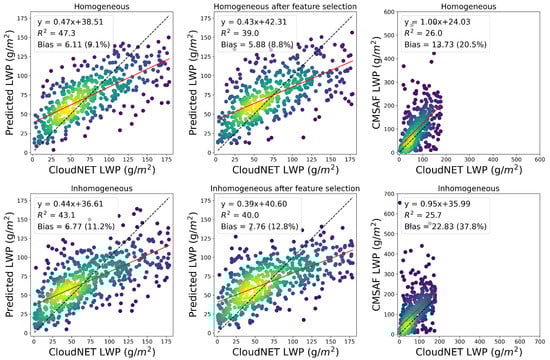
Figure 1.
Scatter plot for homogeneous (upper) and inhomogeneous (lower) situations with no feature selection (left column), with feature selection (middle column), and CM SAF LWP (right column) for Leipzig. Independent test data shown in this figure are a random subset of 33% of the full dataset, and date from 11 August 2011 to 30 November 2015. The red solid line is a line of best fit to the scatter plot, and the black dotted line is an identity line. The color indicates the point density from blue (low) to yellow (high), estimated by a Gaussian kernel density estimation. Note that the axes for the CM SAF LWP plots have different sizes to include all data points.
The bias is a measure of how far the predicted values are from the true values, and used as an indicator of accuracy in this study. It is calculated as the difference between the medians of model-predicted LWP and CloudNet LWP [7]. Percent bias (PB) is calculated by dividing the bias by the median of CloudNet LWP and multiplying it by 100, as in [2,7]. PB represents the average tendency where the predicted values are greater or less than the true ones, with the optimal value of 0. Positive PB values mean model overestimation bias, while negative values model underestimation bias. The PB is found to be around 9%, which is almost the same as that reported by Roebeling et al. [7] (9%) and slightly better than those reported by Greuell and Roebeling [2] (15%) and shown in the CLAAS-2 LWP’s scatter plot (14%). In general, both homogeneous and inhomogeneous situations without feature selection show higher R2 values than those with feature selection for all sites. It may be because the other IR channels that are not used in those with feature selection could give valuable information to obtain a more accurate estimation of LWP, although they contribute much less to the prediction than the other channels, as discussed in Section 3.3. However, the difference is not obvious in the PB values (cf. Table A1 and Table A2).
Figure 2 shows the medians and interquartile range of bias distribution with respect to LWP predicted from the GBRT model and CLAAS-2 for both homogeneous and inhomogeneous cloud fields without feature selection. The bias distributions of both the GBRT model and CLAAS-2 LWP show a tendency of increasing bias with increasing LWP values in general for both homogeneous and inhomogeneous cloud fields without feature selection, which is also observed for those with feature selection (not shown), especially when LWP > 100 g m−2, which was also found by Greuell and Roebeling [2]. Deterioration of performance with increasing LWP values seems to be attributed to the limited samples for large values of LWP, as the number of observations (in red letters) drops substantially.
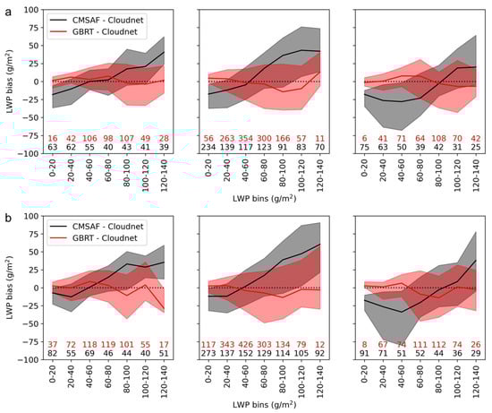
Figure 2.
Median and interquartile range of biases between CloudNet LWP binned by LWP predicted by the GBRT model (red) and CM SAF (black) for: (a) homogeneous cloud fields; and (b) inhomogeneous ones without feature selection for Leipzig (left), Lindenberg (middle), and Juelich (right), respectively. Numbers at the bottom of the panels state number of observations.
3.2. Bias Analysis for LWP Retrieval
The bias was calculated for bins with a width of 20 g m−2 from instantaneous LWP values as a function of CloudNet LWP for test data for homogeneous cloud fields without feature selection at each site as an example (Figure 3). The biases of LWP predicted by the GBRT model increase with increasing CloudNet LWP values, which is also observed for the other cloud fields with and without feature selection. The reduction in accuracy with increasing LWP values has been observed in past studies [2,7]. Roebeling et al. [7] reported an underestimation of about 30 g m−2 of SEVIRI-retrieved LWP at a CloudNet LWP of 100 g m−2. This study is fairly consistent with this, with less than 25 g m−2 underestimation of predicted LWP at 100 g m−2 of CloudNet LWP. The limited number of samples at higher LWP values is likely to contribute to an increased bias especially in the GBRT model. Meanwhile, bias variability (represented by the error bars in the bias plots) is much larger for CLAAS-2 than in the GBRT approach. Figure 4 presents the bias calculated in the same way as for Figure 3 but from daily medians of LWP values. The ground-based instrument observes much smaller areas around nadir than satellite pixel size. Using daily medians may mitigate the effect of spatial mismatch caused by the scale differences between ground-based and satellite observations [7]. In general, using longer LWP-averaging times reduces the bias in this study, which agrees with the findings of Roebeling et al. [7]. They reported that the precision (i.e., variance) of the bias is significantly improved when using the daily LWP values instead of using the instantaneous LWP values. This study shows a reduction in the bias by approximately 17.5% on average when daily LWP values are used.
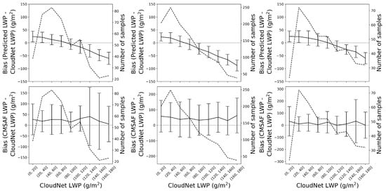
Figure 3.
Bias calculated for bins of 20 g m−2 from instantaneous LWP retrieved by the GBRT model (top) and CLAAS-2 (bottom) as a function of CloudNet LWP for Leipzig (left), Lindenberg (middle), and Juelich (right) for homogeneous cloud fields without feature selection. The error bars are for one standard deviation of samples in each bin. The dotted line indicates the number of samples.
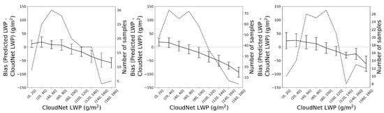
Figure 4.
Bias calculated for bins of 20 g m−2 from daily medians of LWP retrieved by the GBRT model as a function of CloudNet LWP for Leipzig (left), Lindenberg (middle), and Juelich (right) for homogeneous cloud fields without feature selection. The error bars are for one standard deviation of samples in each bin. The dotted line indicates the number of samples.
Figure 5 shows the bias as a function of SZA and AZA for test data for homogeneous situations without feature selection in Leipzig as an example. At the range of SZA > 63°, the bias shows a slight decrease, but not much. Figure 6 demonstrates the bias as a function of hours and months. Bias increases with increasing SZA, during late afternoon and in October and November, when SZA is mostly over 60° or higher, which is consistent with the results of Roebeling et al. [7], who found that LWP from SEVIRI is overestimated at those times relative to CloudNet. It has been reported that at oblique viewing angles cloud properties can be overestimated for both broken and overcast clouds, as reflectances increase much in the forward-scattering direction [7,31]. It should be noted that there is no obvious difference between homogeneous and inhomogeneous cases with and without feature selection for angle and time-dependent errors, which are not shown here.
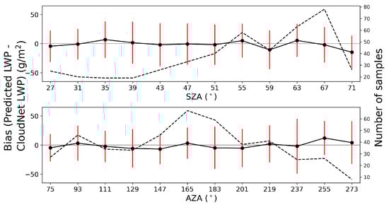
Figure 5.
Angle-dependent error plots as a function of solar zenith angle (top) and azimuth angle (bottom) for test data for homogeneous without feature selection in Leipzig. The black lines are means of the bias between LWP retrieved by the GBRT model and CloudNet LWP with one standard deviation as the red vertical line. The black dashed lines indicate the number of samples.
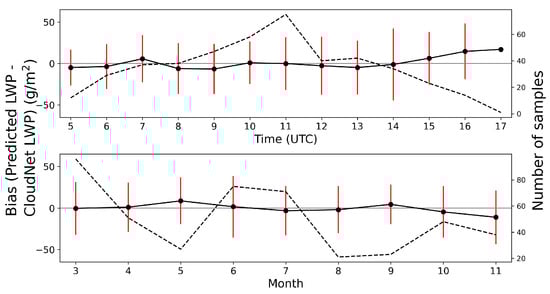
Figure 6.
Time-dependent error plots as a function of hours (top) and months (bottom) for test data for homogeneous without feature selection in Leipzig. The black lines are means of the bias between LWP retrieved by the GBRT model and CloudNet LWP with one standard deviation as the red vertical line. The black dashed lines indicate the number of samples.
3.3. Relationship between LWP and Input Variables
The model input variables and their influence on the model’s predictions are investigated for a better understanding of how the model works. Figure 7 and Figure 8 show the feature importances and the partial dependencies of the GBRT models for the three study sites for without feature selection (Feature Set 1) and with feature selection (Feature Set 2), respectively, for homogeneous cloud fields to get a more reliable analysis. The y-axis of the PD plot shows the relative contribution of the input feature on the prediction. Partial dependence is the average response of an estimator for each possible grid value of the feature (x-axis) based on a weighted tree traversal [25]. It can be interpreted as a relationship between two variables (i.e., input feature and target). For example, positive (negative) values indicate that a specific grid value is corresponding to an increase (decrease) of predicted LWP. The important features identified in the feature importance result on the upper (Figure 7) and the left (Figure 8) can be related to high/obvious partial dependence in the PD plots.
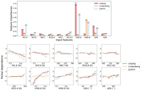
Figure 7.
Feature importance (top) and partial dependence plot (bottom) for training data for homogeneous cloud fields without feature selection. The y-axis of the partial dependence plot shows the changes of LWP (in units of LWP) relative to the mean prediction (centered around zero) for each grid value on the x-axis.
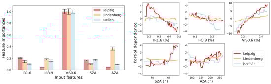
Figure 8.
Feature importance (left) and partial dependence plot (right) for training data for homogeneous cloud fields with feature selection. The y-axis of the partial dependence plot shows the changes of LWP (in units of LWP) relative to the mean prediction (centered around zero) for each grid value on the x-axis.
At all sites, VIS channels appear to be the most important feature for the model’s prediction in Figure 7 and Figure 8. Other IR channels are much less significant to the prediction, which is also visible in the PD plot in Figure 7 with nearly no variations of partial dependence. It was as expected because VIS0.6 related to cloud optical thickness information, IR1.6 and IR3.9 channels, which are changed by the droplet effective radius, are commonly used as input to LWP retrievals [6,7,27]. As shown in the PD plot, the effect of the VIS0.6 on the LWP estimation variable at all sites is clearly seen. The reflectance increases with LWP that might correspond to the increase of the cloud thickness (cf. [32]). Clouds with high LWP tend to have larger droplets that absorb more NIR radiation and thereby lead to a smaller reflectance at the NIR [32]. This is well represented in the PD plots of the IR1.6 and IR3.9 variables. For smaller reflectance in the IR016 and IR039 plots, the model predicts higher LWP values. Compared to the other two sites, Leipzig shows relatively pronounced changes in the partial dependence of the IR 1.6 µm channel in Figure 8. Chang and Li [32] found that, as the reflectance saturates more quickly with greater DER, the dependence of the reflectance on the DER becomes larger as the DER decreases. According to CLAAS-2 DER data, Leipzig is found to have relatively smaller DER values compared to other sites in the selected samples (Figure A1). Furthermore, the longer is the wavelength (1.6 → 3.7), the faster does the signal saturate [32], which may explain why Leipzig shows a stronger partial dependence of LWP on changes in IR1.6 compared to the IR3.9.
Figure 9 shows that CloudNet LWP changes depending on satellite viewing geometry in the left panel and the SHAP interaction values in the right panel. SHAP values are useful for interpreting situations in which each input feature has a different contribution to the prediction, but works with each other to obtain the prediction. Each input feature either increases or decreases the prediction. SHAP interaction values allow visualizing a combined contribution as a feature’s changes with another feature changing. Higher (lower) SHAP interaction values represent higher (lower) LWP predictions with different contributions from two input features. In the PD plots, it was found that SZA has a stronger effect on retrieved LWP particularly at high values for Leipzig and Lindenberg, while AZA shows a less pronounced partial dependence for all stations. The left panel in Figure 9 shows that LWP varies with both SZA and AZA, although this variation only seems to be systematic in the case of AZA. This suggests that the diurnal cycle of LWP cannot explain the relatively strong influence of SZA on LWP predicted by the model. In this case, the angle information can still play a supplementary role in retrieving LWP by interacting with VIS0.6. In the SHAP interaction plot, the interaction of VIS0.6 and SZA has negative contributions on the prediction in general, which means that the combined contribution reduces the predicted LWP values. Meanwhile, for the range of high SZA, high reflectance in VIS0.6 increases the predicted LWP, while low reflectance of VIS0.6 decreases the predicted LWP. It has been reported that retrieved LWP is strongly dependent on solar geometry [7,33]. This has been largely attributed to the COT retrievals, which directly affect LWP retrievals. COT tends to increase with increasing SZA and to be overestimated at SZA > 60. Note that, although SZA has the strongest interaction with VIS0.6, the interaction might be affected by other features, as SZA and LWP are correlated with other NIR channels to some extent.
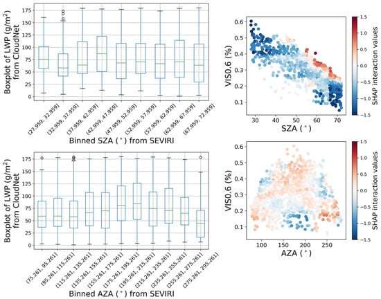
Figure 9.
Box plot (left) of LWP based on SZA and AZA and SHAP interaction values (right) for between LWP and the satellite viewing geometry in Leipzig.
4. Summary and Conclusions
This study presents a machine-learning based technique to retrieve cloud LWP using SEVIRI data. We analyzed the potential of a machine learning approach for designing reliable cloud-property retrievals. A statistical LWP retrieval was developed using spectral information from MSG-2 SEVIRI and satellite viewing geometry. CloudNet ground-based observation data were used to train the model, and CLAAS-2 data as a high-quality reference.
LWP predicted by the GBRT model was validated with independent CloudNet LWP observations in four different situations including homogeneous and inhomogeneous clouds, and both with and without prior selection of input features. During this validation, the skill (R2) of the GBRT approach was found to be higher than that of the physics-based retrieval in all situations. Inhomogeneous situations feature lower R2 values and higher biases in general, but the difference was not as pronounced as expected. The bias distributions of both the GBRT model and CLAAS-2 LWP show a tendency of increasing bias as LWP values increase in general for both homogeneous and inhomogeneous cloud fields, especially for high LWP values. Deterioration of performance with increasing LWP values seems to be attributed to the limited samples for large values of LWP. It was found that both homogeneous and inhomogeneous situations without feature selection show higher R2 values than those with feature selection in general for all sites, but there was no meaningful difference between with and without feature selection in terms of bias.
VIS0.6 has been shown to be the most important feature for the model’s prediction. The corresponding partial dependence plot also presents the clear dependence of LWP estimation on VIS0.6 at all sites. Meanwhile, LWP values increase with increasing droplet size as more radiation is absorbed by the droplets, leading to smaller reflectance in the NIR. This is well observed in the partial dependence plots. For lower reflectances in IR1.6 and IR3.9, the model predicts higher LWP values. The magnitude of this dependence is site-specific. Leipzig has stronger changes in the partial dependence of the IR 1.6 µm channel than the other two sites. As the reflectance saturates more quickly with larger DER, the dependence of the reflectance on the DER can be larger as the DER decreases. This is indirectly identified by CLAAS-2 DER with Leipzig having relatively smaller DER values than the other sites. SZA and AZA variables have a relatively low importance in the feature importance results, but it is shown that SZA has a strong interaction with VIS0.6 in the SHAP interaction plots. Overall, the interaction of VIS0.6 and SZA has a negative effect on the prediction, but a positive effect of the interaction on LWP prediction is observed for high SZA values as well.
The biases of instantaneous LWP values predicted by GBRT model increase with increasing CloudNet LWP values, which is due to limited samples at larger LWP. Error bars of the bias are much wider in CLAAS-2 compared to GBRT model. The bias from daily median LWP values shows that using longer LWP averaging times reduces the bias, which is consistent with past studies, as spatial mismatch caused by spatial scale difference between ground-based and satellite observations could be mitigated by using daily values instead of using instantaneous values. The bias tends to become negative (i.e., predicted LWP larger than CloudNet LWP) with increasing SZA. It was also found that time-dependent errors increase in late afternoon.
The results suggests that the LWP retrieved by the machine-learning model is useful, as it is in good agreement with ground-based reference measurements. In the cases and locations considered here its overall performance relative to CloudNet was better than the state-of-the-art physics-based CLAAS-2 product. Nevertheless, transferability to sites outside Germany and potentially different conditions would have to be tested. In addition, while CLAAS-2 is aimed at representing all clouds, a particular focus and filter was implemented in the approach presented here. Overall, the results highlight the potential of cloud-property retrievals based on machine learning.
Author Contributions
M.K. and J.C. developed the idea. M.K. collected and analyzed the data, conducted the research experiments, and wrote the manuscript. M.K., J.C., H.A., J.F. and R.S. contributed to research design, manuscript preparation, and the interpretation of the results. All authors have read and agreed to the published version of the manuscript.
Funding
This research partly belongs to the FORCeS project that has received funding from the European Union’s Horizon 2020 research and innovation programme under grant agreement No 821205.
Acknowledgments
We acknowledge the use of CloudNet data which are part of the European Aerosol, Clouds and Trace Gases Research Infrastructure (ACTRIS) project. We acknowledge support by the KIT-Publication Fund of the Karlsruhe Institute of Technology.
Conflicts of Interest
The authors declare they have no conflict of interest.
Appendix A
Table A1.
Summary of the relation between LWPGBRT and LWPgr for test data for each site in different situations. n is the total number of samples.
Table A1.
Summary of the relation between LWPGBRT and LWPgr for test data for each site in different situations. n is the total number of samples.
| Situations | Sites | Linear Relation of LWPGBRT − LWPgr | |||
|---|---|---|---|---|---|
| n | R2 (%) | Slope | Intercept (g m−2) | ||
| Homogeneous | Leipzig | 450 | 47.3 | 0.47 | 38.51 |
| Lindenberg | 1207 | 34.1 | 0.33 | 36.76 | |
| Juelich | 412 | 46.4 | 0.46 | 43.67 | |
| Homogeneous after feature selection | Leipzig | 450 | 39.0 | 0.43 | 42.31 |
| Lindenberg | 1207 | 20.3 | 0.20 | 44.26 | |
| Juelich | 412 | 37.6 | 0.32 | 54.46 | |
| Inhomogeneous | Leipzig | 528 | 43.0 | 0.44 | 36.61 |
| Lindenberg | 1415 | 31.3 | 0.31 | 34.64 | |
| Juelich | 482 | 35.9 | 0.38 | 44.78 | |
| Inhomogeneous after feature selection | Leipzig | 528 | 40.0 | 0.39 | 40.60 |
| Lindenberg | 1415 | 20.0 | 0.17 | 42.19 | |
| Juelich | 482 | 28.7 | 0.30 | 49.88 | |
| Linear Relation of LWPCMSAF − LWPgr | |||||
| Homogeneous | Leipzig | 450 | 26.0 | 1.00 | 24.03 |
| Lindenberg | 1202 | 12.9 | 0.91 | 51.57 | |
| Juelich | 412 | 18.6 | 0.95 | 18.28 | |
| Inhomogeneous | Leipzig | 528 | 25.7 | 0.95 | 35.99 |
| Lindenberg | 1411 | 12.1 | 0.90 | 57.97 | |
| Juelich | 482 | 9.5 | 0.90 | 28.33 | |
Table A2.
Statistics for comparison between LWPGBRT and LWPgr for test data for each site in different situations. Q50, Q66, and Q95 are calculated as the difference between the 25th/17th/2.5th and 75th/83rd/97.5th percentiles of the difference between CloudNet LWP and GBRT-predicted LWP, respectively. Units are g m−2 for mean, median, Q50, Q66, and Q95.
| Situations | Sites | Difference between LWPGBRT and LWPgr | |||||||
|---|---|---|---|---|---|---|---|---|---|
| Mean (GBRT) | Mean (gr) | Median (GBRT) | Median (gr) | Accuracy (PB%) | Q50 (Prec) | Q66 | Q95 | ||
| Homogeneous | Leipzig | 73.38 | 74.42 | 72.98 | 66.87 | 6.11 (9.14) | 40.01 | 59.49 | 131.44 |
| Lindenberg | 57.80 | 64.27 | 56.23 | 54.63 | 1.60 (2.93) | 46.46 | 65.25 | 144.39 | |
| Juelich | 81.89 | 83.34 | 85.32 | 78.89 | 6.43 (8.15) | 42.40 | 66.38 | 130.20 | |
| Homogeneous after feature selection | Leipzig | 74.40 | 74.42 | 72.75 | 66.87 | 5.88 (8.79) | 39.37 | 60.25 | 141.88 |
| Lindenberg | 56.81 | 64.27 | 54.41 | 54.63 | −0.22 (0.40) | 58.77 | 77.65 | 146.24 | |
| Juelich | 81.25 | 83.34 | 86.12 | 78.89 | 7.23 (9.16) | 53.69 | 76.55 | 138.57 | |
| Inhomogeneous | Leipzig | 67.53 | 69.92 | 67.24 | 60.47 | 6.77 (11.20) | 40.98 | 59.13 | 149.26 |
| Lindenberg | 54.10 | 62.03 | 52.16 | 51.73 | 0.43 (0.83) | 47.96 | 71.84 | 151.74 | |
| Juelich | 76.10 | 81.76 | 76.96 | 77.30 | −0.33 (0.43) | 50.20 | 73.37 | 148.12 | |
| Inhomogeneous after feature selection | Leipzig | 67.53 | 69.92 | 68.23 | 60.47 | 7.76 (12.83) | 45.89 | 66.72 | 152.95 |
| Lindenberg | 52.88 | 62.03 | 51.12 | 51.73 | −0.60 (1.17) | 58.95 | 83.36 | 152.11 | |
| Juelich | 74.49 | 81.76 | 76.07 | 77.30 | −1.23 (1.59) | 57.06 | 79.42 | 153.06 | |
| Difference between LWPCMSAF and LWPgr | |||||||||
| Homogeneous | Leipzig | 98.27 | 74.42 | 80.60 | 66.87 | 13.73 (20.53) | 58.40 | 85.55 | 273.97 |
| Lindenberg | 110.12 | 64.27 | 77.50 | 54.63 | 22.87 (41.86) | 92.46 | 140.74 | 368.75 | |
| Juelich | 97.35 | 83.34 | 66.20 | 78.89 | −12.69 (16.09) | 63.28 | 108.42 | 359.40 | |
| Inhomogeneous | Leipzig | 102.64 | 69.92 | 83.30 | 60.47 | 22.83 (37.76) | 57.89 | 89.87 | 276.40 |
| Lindenberg | 113.68 | 62.03 | 81.80 | 51.73 | 30.07 (58.14) | 96.34 | 141.95 | 403.75 | |
| Juelich | 101.87 | 81.76 | 69.70 | 77.30 | −7.60 (9.83) | 69.93 | 114.32 | 345.44 | |

Figure A1.
Droplet effective radius derived from CM SAF CLAAS-2 for test data for the study sites.
Figure A1.
Droplet effective radius derived from CM SAF CLAAS-2 for test data for the study sites.

References
- Boucher, O.; Randall, D.; Artaxo, P.; Bretherton, C.; Feingold, G.; Forster, P.; Kerminen, V.M.; Kondo, Y.; Liao, H.; Lohmann, U.; et al. Clouds and aerosols. In Climate Change 2013: The Physical Science Basis. Contribution of Working Group I to the Fifth Assessment Report of the Intergovernmental Panel on Climate Change; Cambridge University Press: Cambridge, UK, 2013; pp. 571–657. [Google Scholar]
- Greuell, W.; Roebeling, R. Toward a standard procedure for validation of satellite-derived cloud liquid water path: A study with SEVIRI data. J. Appl. Meteorol. Climatol. 2009, 48, 1575–1590. [Google Scholar] [CrossRef]
- Hollmann, R.; Merchant, C.J.; Saunders, R.; Downy, C.; Buchwitz, M.; Cazenave, A.; Chuvieco, E.; Defourny, P.; de Leeuw, G.; Forsberg, R.; et al. The ESA climate change initiative: Satellite data records for essential climate variables. Bull. Am. Meteorol. Soc. 2013, 94, 1541–1552. [Google Scholar] [CrossRef]
- Roebeling, R.; Feijt, A.; Stammes, P. Cloud property retrievals for climate monitoring: Implications of differences between Spinning Enhanced Visible and Infrared Imager (SEVIRI) on METEOSAT-8 and Advanced Very High Resolution Radiometer (AVHRR) on NOAA-17. J. Geophys. Res. Atmos. 2006, 111. [Google Scholar] [CrossRef]
- O’Dell, C.W.; Wentz, F.J.; Bennartz, R. Cloud liquid water path from satellite-based passive microwave observations: A new climatology over the global oceans. J. Clim. 2008, 21, 1721–1739. [Google Scholar] [CrossRef]
- Seethala, C.; Horváth, Á. Global assessment of AMSR-E and MODIS cloud liquid water path retrievals in warm oceanic clouds. J. Geophys. Res. Atmos. 2010, 115. [Google Scholar] [CrossRef]
- Roebeling, R.; Deneke, H.; Feijt, A. Validation of cloud liquid water path retrievals from SEVIRI using one year of CloudNET observations. J. Appl. Meteorol. Climatol. 2008, 47, 206–222. [Google Scholar] [CrossRef]
- Kniffka, A.; Stengel, M.; Lockhoff, M.; Bennartz, R.; Hollmann, R. Characteristics of cloud liquid water path from SEVIRI onboard the Meteosat Second Generation 2 satellite for several cloud types. Atmos. Meas. Tech. 2014, 7, 887–905. [Google Scholar] [CrossRef]
- Kostsov, V.S.; Kniffka, A.; Stengel, M.; Ionov, D.V. Cross-comparison of cloud liquid water path derived from observations by two space-borne and one ground-based instrument in northern Europe. Atmos. Meas. Tech. 2019, 12, 5927–5946. [Google Scholar] [CrossRef]
- Schutgens, N.; Roebeling, R. Validating the validation: The influence of liquid water distribution in clouds on the intercomparison of satellite and surface observations. J. Atmos. Ocean. Technol. 2009, 26, 1457–1474. [Google Scholar] [CrossRef]
- Greenwald, T.J.; Bennartz, R.; Lebsock, M.; Teixeira, J. An uncertainty data set for passive microwave satellite observations of warm cloud liquid water path. J. Geophys. Res. Atmos. 2018, 123, 3668–3687. [Google Scholar] [CrossRef]
- Müller, J.; Fowler, G.; Dammann, K.; Rogers, C.; Buhler, Y.; Flewin, J. MSG Level 1.5 Image Data Format Description; Rapport Technique; EUMETSAT: Darmstadt, Germany, 2010; Volume 68, p. 167. [Google Scholar]
- SAF, C. Algorithm Theoretical Basis Document, SEVIRI Cloud Physical Products, CLAAS Edition 2, EUMETSAT Satellite Application Facility on Climate Monitoring; Technical Report, SAF/CM/KNMI/ATBD/SEVIRI/CPP; Satellite Application Facility on Climate Monitoring (CM SAF): Darmstadt, Germany, 2016. [Google Scholar]
- Cermak, J.; Bendix, J. A novel approach to fog/low stratus detection using Meteosat 8 data. Atmos. Res. 2008, 87, 279–292. [Google Scholar] [CrossRef]
- Strabala, K.I.; Ackerman, S.A.; Menzel, W.P. Cloud Properties inferred from 8–12-µm Data. J. Appl. Meteorol. 1994, 33, 212–229. [Google Scholar] [CrossRef]
- Illingworth, A.; Hogan, R.; O’connor, E.; Bouniol, D.; Brooks, M.; Delanoë, J.; Donovan, D.; Eastment, J.; Gaussiat, N.; Goddard, J.; et al. Cloudnet: Continuous evaluation of cloud profiles in seven operational models using ground-based observations. Bull. Am. Meteorol. Soc. 2007, 88, 883–898. [Google Scholar] [CrossRef]
- Löhnert, U.; Crewell, S. Accuracy of cloud liquid water path from ground-based microwave radiometry 1. Dependency on cloud model statistics. Radio Sci. 2003, 38. [Google Scholar] [CrossRef]
- Gaussiat, N.; Hogan, R.J.; Illingworth, A.J. Accurate liquid water path retrieval from low-cost microwave radiometers using additional information from a lidar ceilometer and operational forecast models. J. Atmos. Ocean. Technol. 2007, 24, 1562–1575. [Google Scholar] [CrossRef]
- Finkensieper, S.; Meirink, J.; van Zadelhoff, G.; Hanschmann, T.; Benas, N.; Stengel, M.; Fuchs, P.; Hollmann, R.; Werscheck, M. CLAAS-2: CM SAF CLoud Property dAtAset Using SEVIRI, 2nd ed.; Satellite Application Facility on Climate Monitoring: Darmstadt, Germany, 2016. [Google Scholar]
- Stephens, G.L. Radiation Profiles in Extended Water Clouds. II: Parameterization Schemes. J. Atmos. Sci. 1978, 35, 2123–2132. [Google Scholar] [CrossRef]
- Benas, N.; Finkensieper, S.; Stengel, M.; van Zadelhoff, G.J.; Hanschmann, T.; Hollmann, R.; Meirink, J.F. The MSG-SEVIRI-based cloud property data record CLAAS-2. Earth Syst. Sci. Data 2017, 9, 415. [Google Scholar] [CrossRef]
- Tranquilli, C.; Viticchiè, B.; Pessina, S.; Hewison, T.; Müller, J.; Wagner, S. Meteosat SEVIRI Performance Characterisation and Calibration with Dedicated Moon/Sun/Deep-space Scans. In Proceedings of the 14th International Conference on Space Operations, Daejeon, Korea, 16–20 May 2016; p. 2536. [Google Scholar]
- Aminou, D.M.A.; Jacquet, B.; Pasternak, F. Characteristics of the Meteosat Second Generation (MSG) radiometer/imager: SEVIRI. Sensors, Systems, and Next-Generation Satellites. Int. Soc. Opt. Photonics 1997, 3221, 19–31. [Google Scholar]
- Fuchs, J.; Cermak, J.; Andersen, H. Building a cloud in the southeast Atlantic: Understanding low-cloud controls based on satellite observations with machine learning. Atmos. Chem. Phys. 2018, 18, 16537–16552. [Google Scholar] [CrossRef]
- Friedman, J.H. Greedy function approximation: A gradient boosting machine. Ann. Stat. 2001, 29, 1189–1232. [Google Scholar] [CrossRef]
- Pedregosa, F.; Varoquaux, G.; Gramfort, A.; Michel, V.; Thirion, B.; Grisel, O.; Blondel, M.; Prettenhofer, P.; Weiss, R.; Dubourg, V.; et al. Scikit-learn: Machine learning in Python. J. Mach. Learn. Res. 2011, 12, 2825–2830. [Google Scholar]
- Roebeling, R.; Van Meijgaard, E. Evaluation of the daylight cycle of model-predicted cloud amount and condensed water path over Europe with observations from MSG SEVIRI. J. Clim. 2009, 22, 1749–1766. [Google Scholar] [CrossRef]
- Box, G.E.; Cox, D.R. An analysis of transformations. J. R. Stat. Soc. Ser. B Methodol. 1964, 26, 211–243. [Google Scholar] [CrossRef]
- Breiman, L. Random forests. Mach. Learn. 2001, 45, 5–32. [Google Scholar] [CrossRef]
- Lundberg, S.M.; Lee, S.I. A Unified Approach to Interpreting Model Predictions. In Advances in Neural Information Processing Systems 30; Guyon, I., Luxburg, U.V., Bengio, S., Wallach, H., Fergus, R., Vishwanathan, S., Garnett, R., Eds.; Curran Associates, Inc.: New York, NY, USA, 2017; pp. 4765–4774. [Google Scholar]
- Loeb, N.G.; Coakley, J., Jr. Inference of marine stratus cloud optical depths from satellite measurements: Does 1D theory apply? J. Clim. 1998, 11, 215–233. [Google Scholar] [CrossRef]
- Chang, F.L.; Li, Z. Estimating the vertical variation of cloud droplet effective radius using multispectral near-infrared satellite measurements. J. Geophys. Res. Atmos. 2002, 107, AAC-7. [Google Scholar] [CrossRef]
- Greenwald, T.J. A 2 year comparison of AMSR-E and MODIS cloud liquid water path observations. Geophys. Res. Lett. 2009, 36. [Google Scholar] [CrossRef]


Publisher’s Note: MDPI stays neutral with regard to jurisdictional claims in published maps and institutional affiliations. |
© 2020 by the authors. Licensee MDPI, Basel, Switzerland. This article is an open access article distributed under the terms and conditions of the Creative Commons Attribution (CC BY) license (http://creativecommons.org/licenses/by/4.0/).