
Horizon Line Detection in Historical Terrestrial Images in Mountainous Terrain Based on the Region Covariance


Abstract
1. Introduction
- Taken up to 100 years ago with the earliest available compact cameras, historical images have a poorer image quality resulting in blurred images, low contrasts, and overexposed regions.
- Most images found in archives were acquired from private collections. As those images have not been stored professionally, they show varying signs of usage (e.g., dirt, scratches, watermarks).
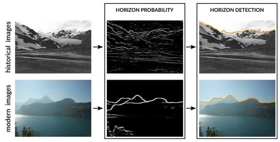
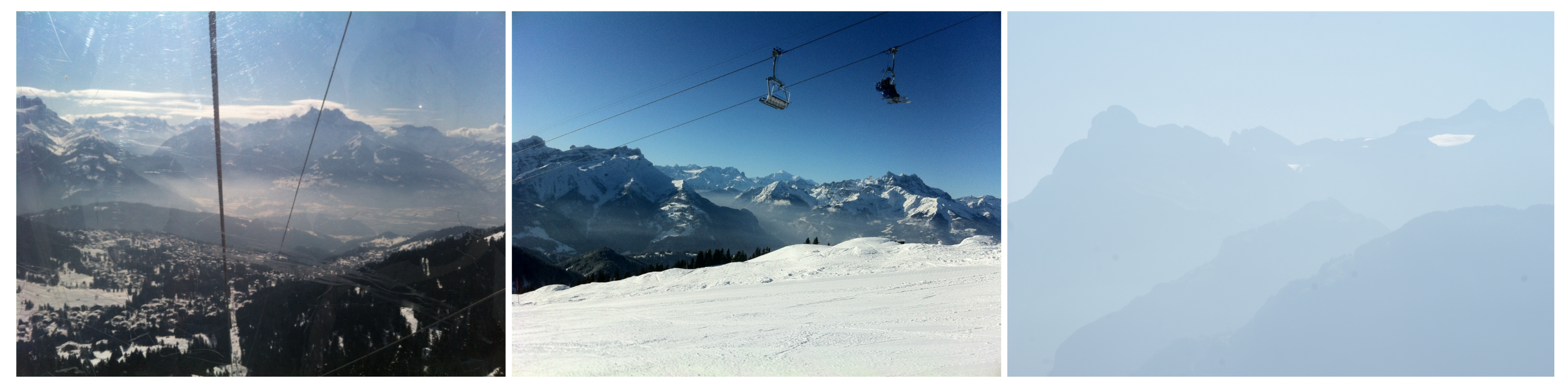
- Alpine environments, even with modern cameras, pose a challenging environment for photography. Especially snow and glacial areas are difficult to photograph due to strongly varying illumination. In combination with rapidly changing weather (e.g., fog, clouds) conditions, visual appearance is heavily affected.
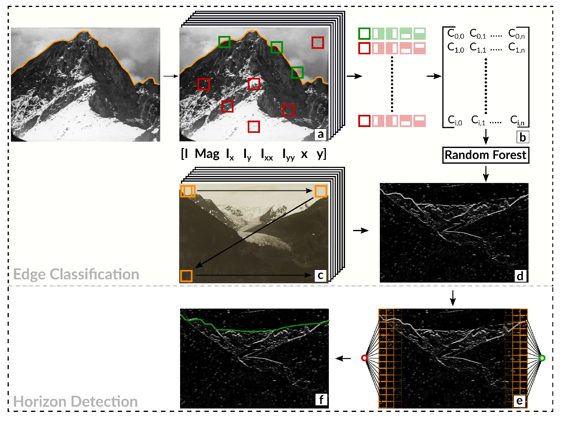
2. Method
2.1. Region Covariance
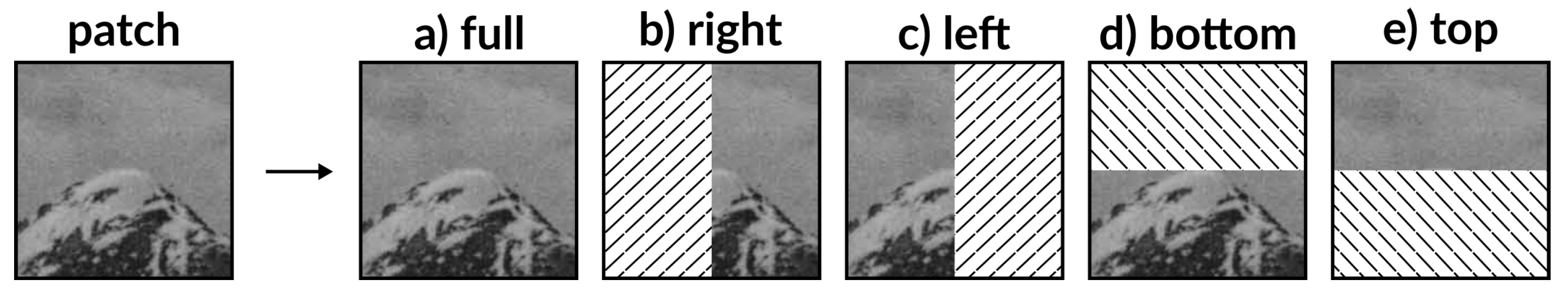
2.1.1. Patch Representation
2.1.2. Classification
2.2. Horizon Line Detection
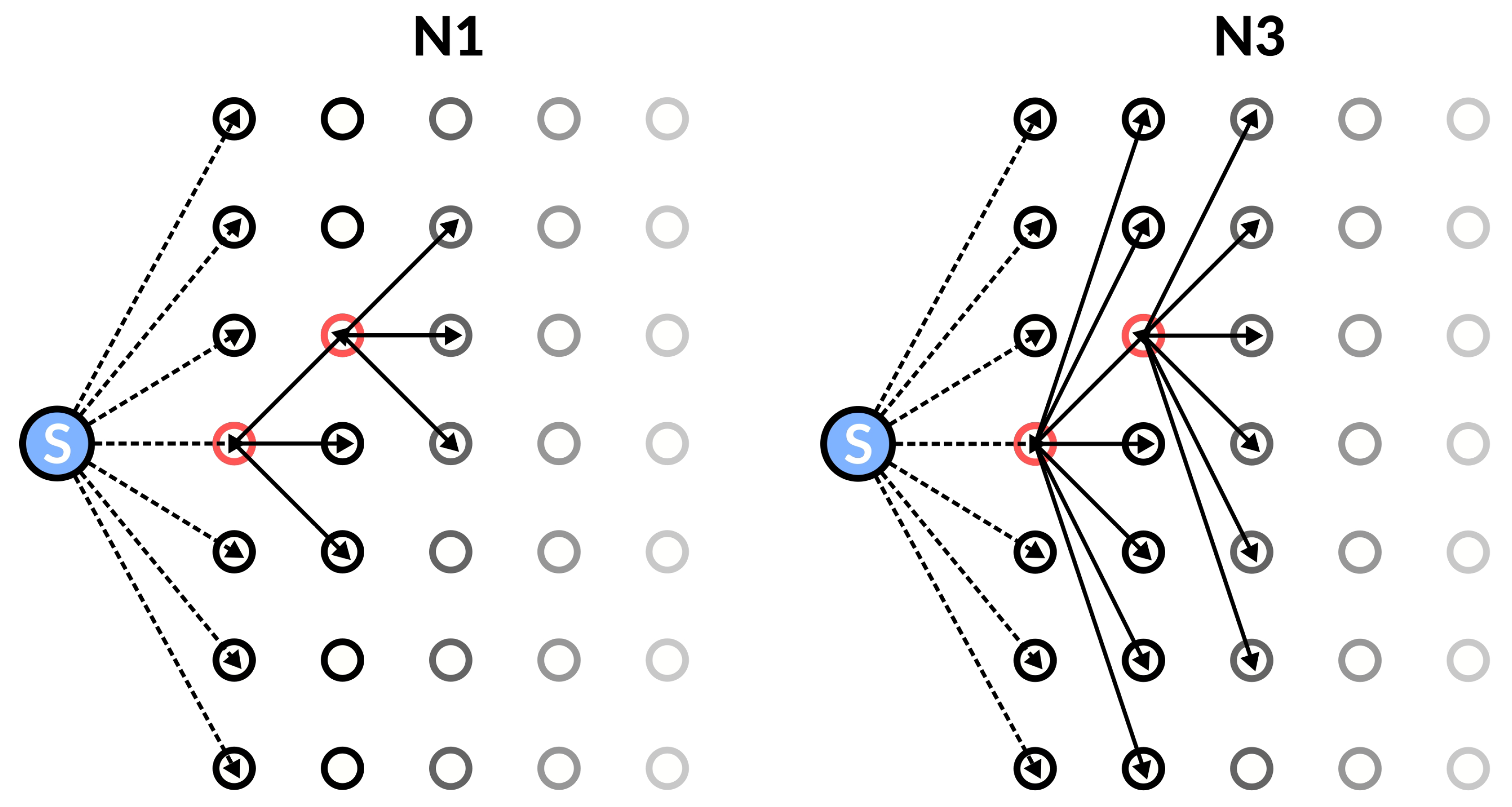
2.2.1. Neighborhood Definition
2.2.2. Edge Weight
2.3. Evaluation
3. Datasets
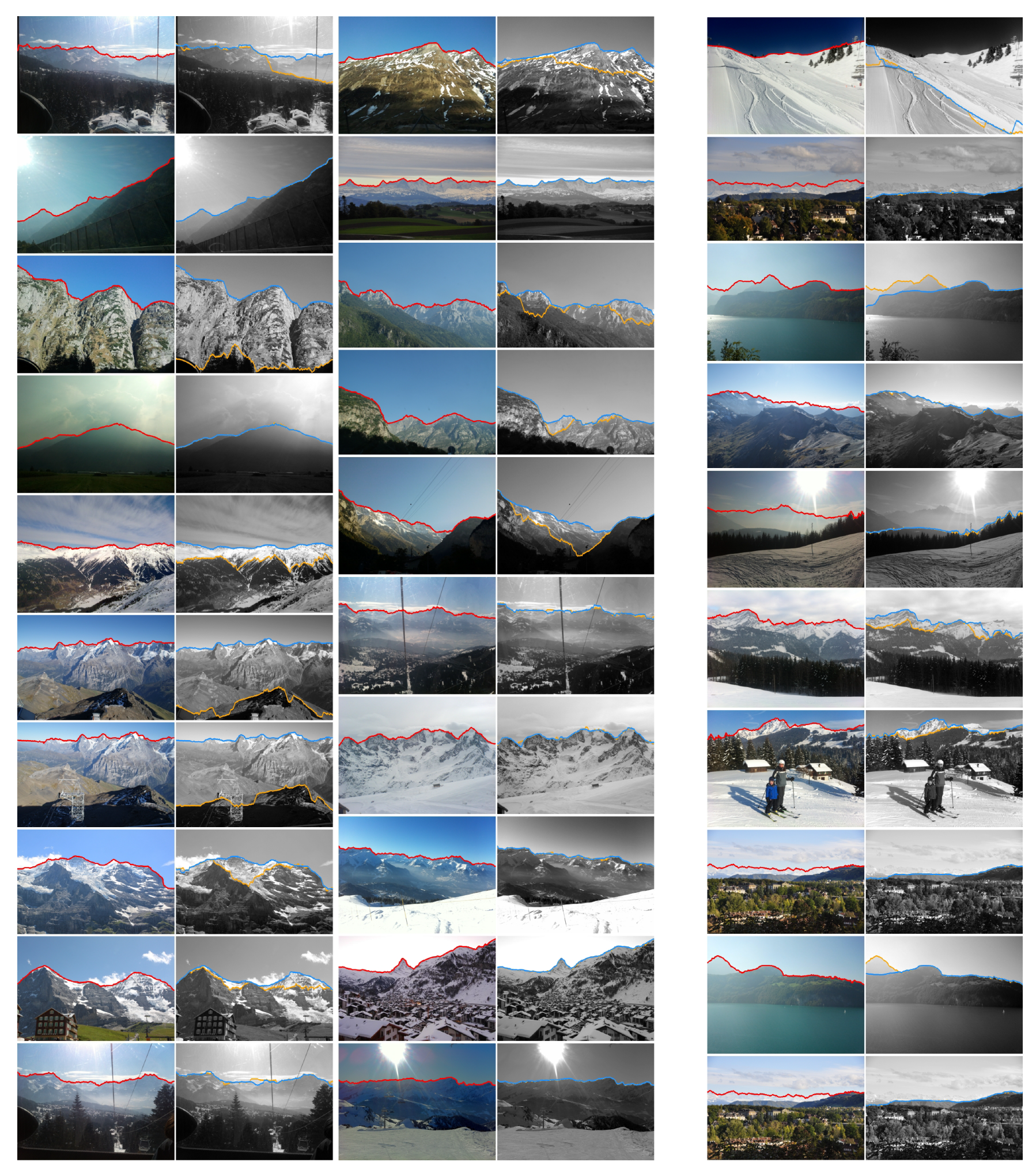
3.1. CH1
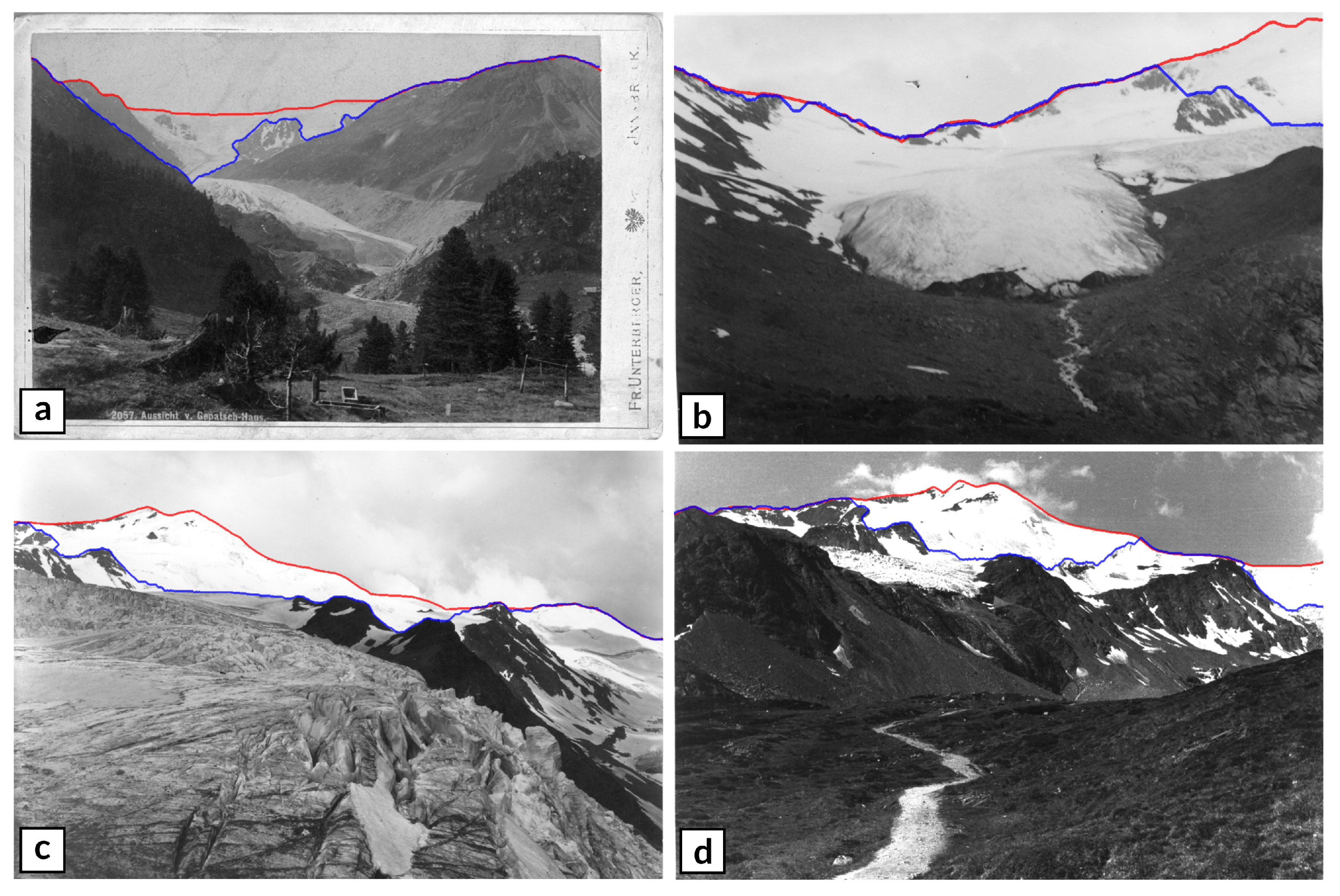
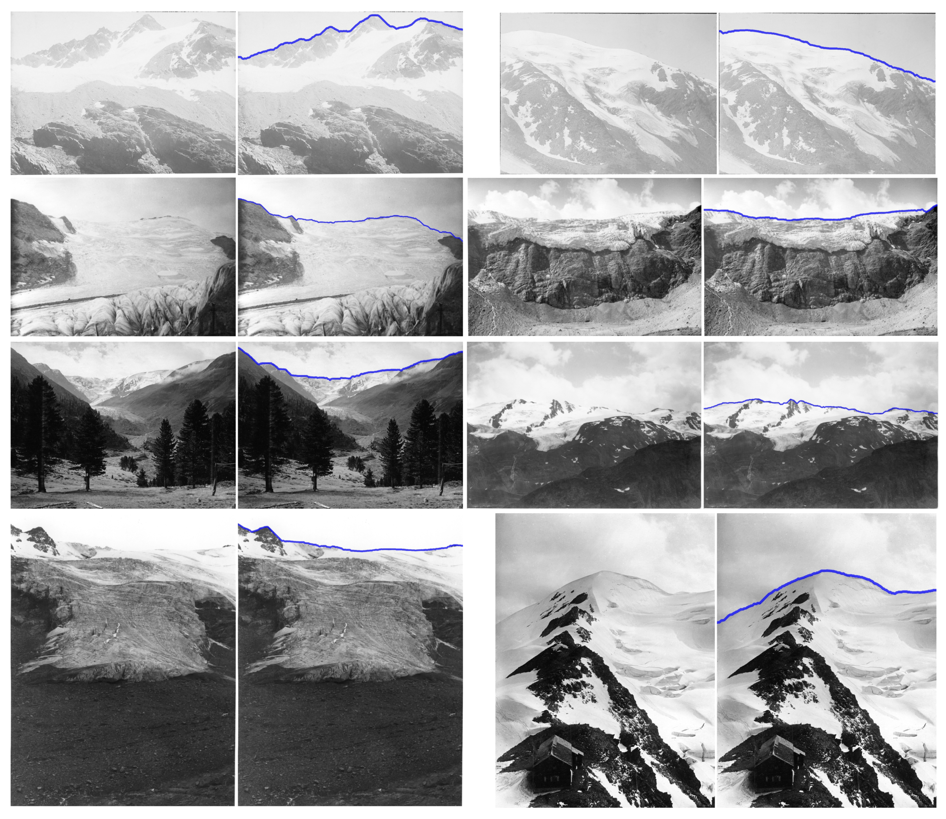
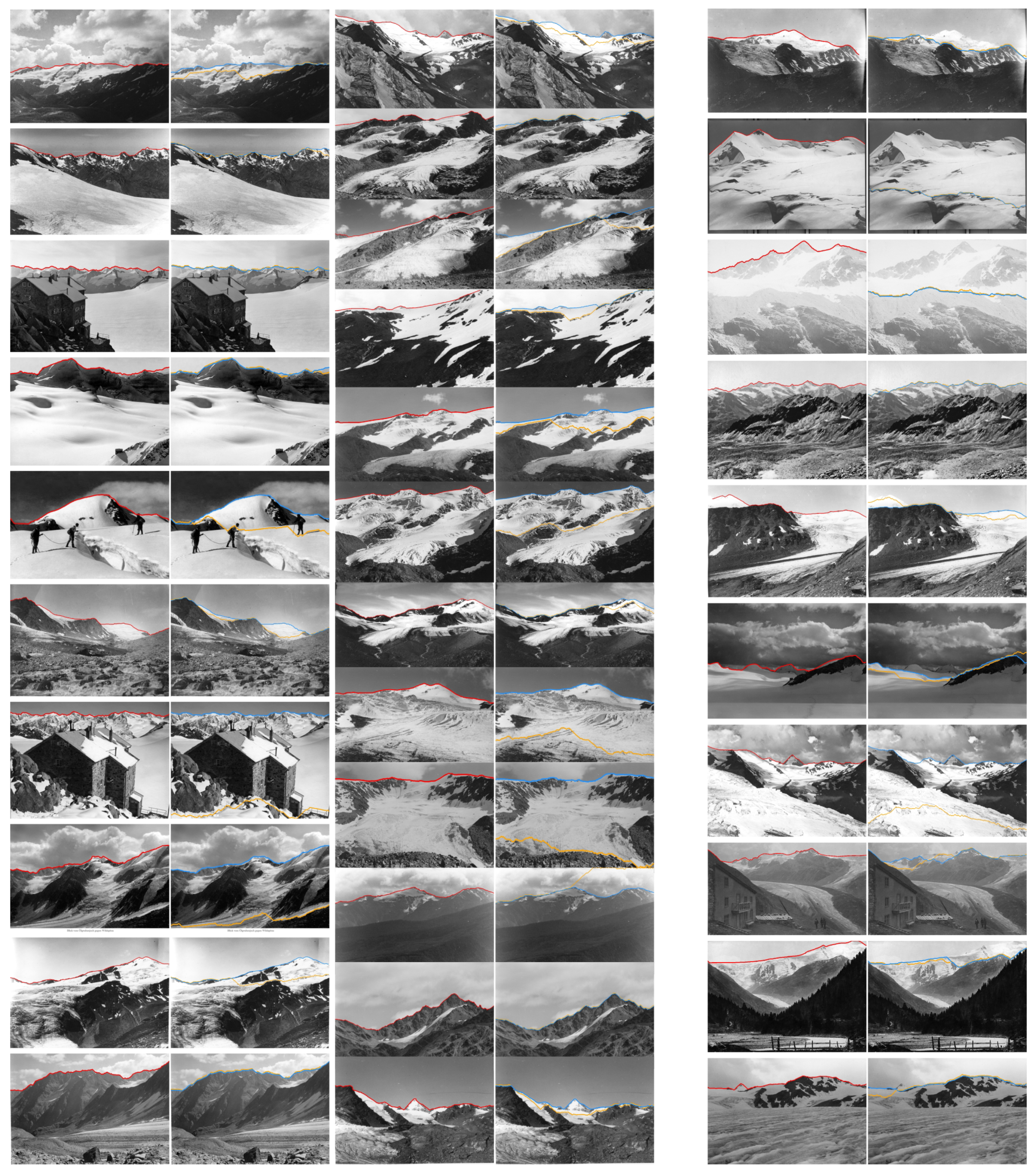
3.2. HIST
4. Results
4.1. CH1
- DCNN-DS1: Fully convolutional network proposed in [16];
- SVM: Patch classification using normalized gray-scale values [14];
- CNN: Convolutional neural network trained on patches proposed in [14];
- Structured Forest: Learned edge detection proposed in [32];
- Random Ferns: Learned edge detection proposed in [33].
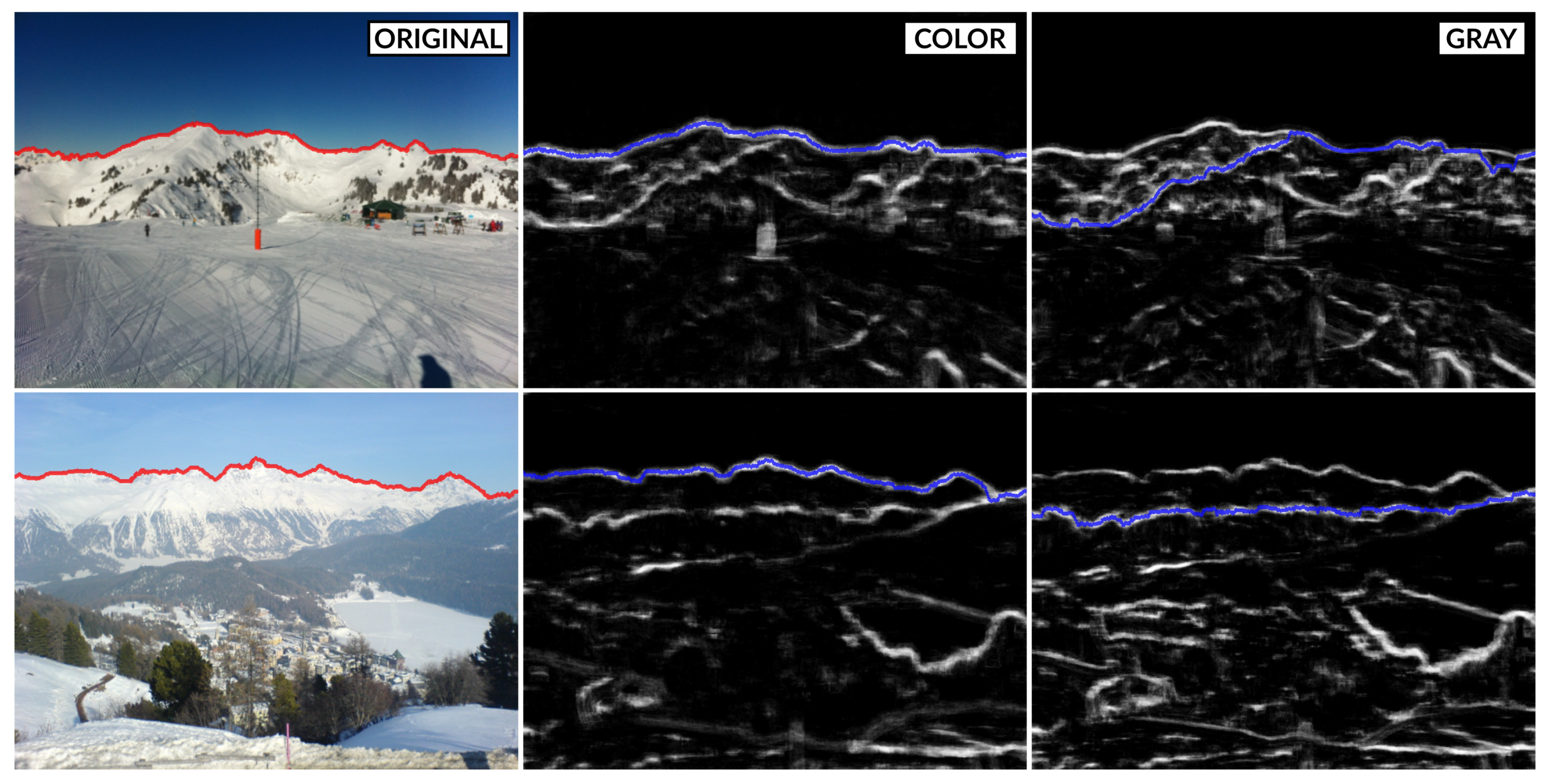
4.1.1. Influence of Color
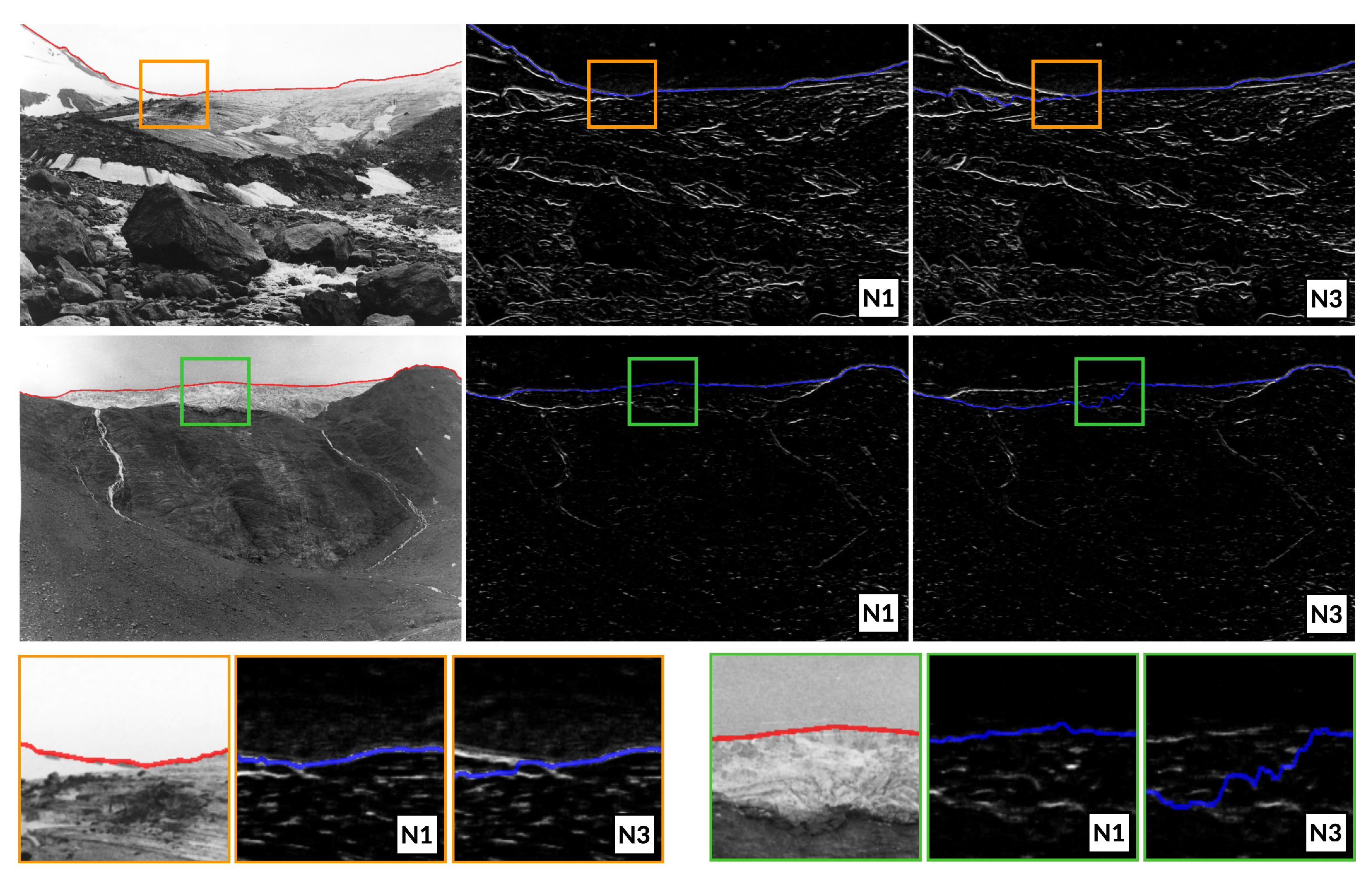
4.1.2. Influence of the Neighborhood DEFINITION
4.1.3. Influence of Step-Size
4.2. HIST
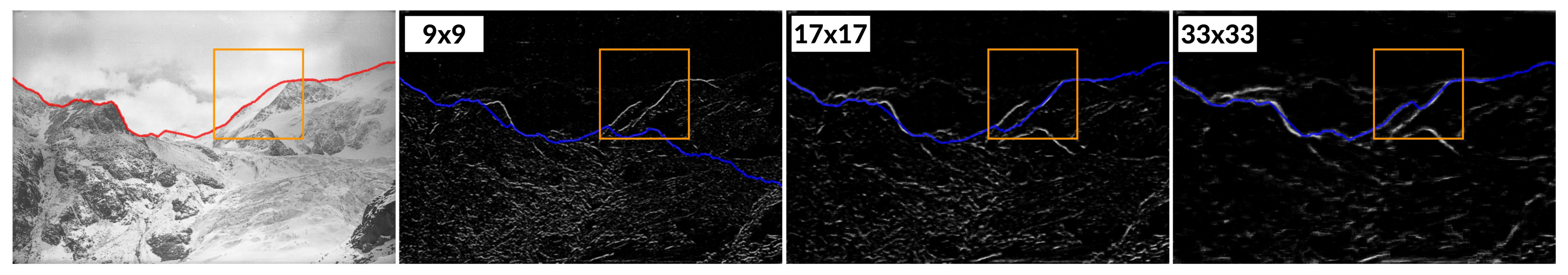
Influence of the PATCH Size
5. Discussion
6. Conclusions
Author Contributions
Funding
Conflicts of Interest
Appendix A. Detected Horizon Lines on the CH1 Dataset

Appendix B. Detected Horizon Lines on the HIST Dataset

References
- Bozzini, C.; Conedera, M.; Krebs, P. A New Monoplotting Tool to Extract Georeferenced Vector Data and Orthorectified Raster Data from Oblique Non-Metric Photographs. Int. J. Herit. Digit. Era 2012, 1, 499–518. [Google Scholar] [CrossRef]
- Lowe, D.G. Distinctive Image Features from Scale-Invariant Keypoints. Int. J. Comput. Vis. 2004, 60, 91–110. [Google Scholar] [CrossRef]
- Bay, H.; Tuytelaars, T.; Van Gool, L. SURF: Speeded Up Robust Features. In Proceedings of the Computer Vision—ECCV 2006, Graz, Austria, 7–13 May 2006; pp. 404–417. [Google Scholar] [CrossRef]
- Rublee, E.; Rabaud, V.; Konolige, K.; Bradski, G. ORB: An efficient alternative to SIFT or SURF. In Proceedings of the 2011 International Conference on Computer Vision, Barcelona, Spain, 6–13 November 2011; pp. 2564–2571. [Google Scholar] [CrossRef]
- Produit, T.; Tuia, D.; Golay, F.; Strecha, C. Pose estimation of landscape images using DEM and orthophotos. In Proceedings of the 2012 International Conference on Computer Vision in Remote Sensing, Xiamen, China, 16–18 December 2012; pp. 209–214. [Google Scholar] [CrossRef]
- Gat, C.; Albu, A.B.; German, D.; Higgs, E. A Comparative Evaluation of Feature Detectors on Historic Repeat Photography. In Advances in Visual Computing; Bebis, G., Boyle, R., Parvin, B., Koracin, D., Wang, S., Kyungnam, K., Benes, B., Moreland, K., Borst, C., DiVerdi, S., et al., Eds.; Lecture Notes in Computer Science; Springer: Berlin/Heidelberg, Germany, 2011; pp. 701–714. [Google Scholar] [CrossRef]
- Baatz, G.; Saurer, O.; Köser, K.; Pollefeys, M. Large Scale Visual Geo-Localization of Images in Mountainous Terrain. In Proceedings of the Computer Vision—ECCV 2012, Florence, Italy, 7–13 October 2012; pp. 517–530. [Google Scholar] [CrossRef]
- Baboud, L.; Čadík, M.; Eisemann, E.; Seidel, H. Automatic photo-to-terrain alignment for the annotation of mountain pictures. In Proceedings of the CVPR 2011, Colorado Springs, CO, USA, 20–25 June 2011; pp. 41–48. [Google Scholar] [CrossRef]
- Cozman, F.; Krotkov, E. Position estimation from outdoor visual landmarks for teleoperation of lunar rovers. In Proceedings of the Third IEEE Workshop on Applications of Computer Vision, WACV’96, Sarasota, FL, USA, 2–4 December 1996; pp. 156–161. [Google Scholar] [CrossRef]
- Naval, P.; Mukunoki, M.; Minoh, M.; Ikeda, K. Estimating Camera Position and Orientation from Geographical Map and Mountain Image. In 38th Research Meeting of the Pattern Sensing Group, Society of Instrument and Control Engineers; Citeseer: Tokyo, Japan, 1997. [Google Scholar]
- Stein, F.; Medioni, G. Map-based localization using the panoramic horizon. IEEE Trans. Robot. Autom. 1995, 11, 892–896. [Google Scholar] [CrossRef]
- Saurer, O.; Baatz, G.; Köser, K.; Ladický, L.; Pollefeys, M. Image Based Geo-localization in the Alps. Int. J. Comput. Vis. 2016, 116, 213–225. [Google Scholar] [CrossRef]
- Lie, W.N.; Lin, T.C.I.; Lin, T.C.; Hung, K.S. A robust dynamic programming algorithm to extract skyline in images for navigation. Pattern Recognit. Lett. 2005, 26, 221–230. [Google Scholar] [CrossRef]
- Ahmad, T.; Bebis, G.; Nicolescu, M.; Nefian, A.; Fong, T. An Edge-Less Approach to Horizon Line Detection. In Proceedings of the 2015 IEEE 14th International Conference on Machine Learning and Applications (ICMLA), Miami, FL, USA, 9–11 December 2015; pp. 1095–1102. [Google Scholar] [CrossRef]
- Frajberg, D.; Fraternali, P.; Torres, R.N. Convolutional Neural Network for Pixel-Wise Skyline Detection. In Proceedings of the Artificial Neural Networks and Machine Learning—ICANN, Alghero, Italy, 11–14 September 2017; pp. 12–20. [Google Scholar] [CrossRef]
- Porzi, L.; Rota Bulò, S.; Ricci, E. A Deeply-Supervised Deconvolutional Network for Horizon Line Detection. In Proceedings of the 24th ACM International Conference on Multimedia, Amsterdam, The Netherlands, 15–19 October 2016. [Google Scholar] [CrossRef]
- Shen, Y.; Wang, Q. Sky Region Detection in a Single Image for Autonomous Ground Robot Navigation. Int. J. Adv. Robot. Syst. 2013, 10, 362. [Google Scholar] [CrossRef]
- Tuzel, O.; Porikli, F.; Meer, P. Region Covariance: A Fast Descriptor for Detection and Classification. In Proceedings of the Computer Vision—ECCV 2006, Graz, Austria, 7–13 May 2006; pp. 589–600. [Google Scholar] [CrossRef]
- Ojala, T.; Pietikäinen, M.; Mäenpää, T. Gray Scale and Rotation Invariant Texture Classification with Local Binary Patterns. Lect. Notes Comput. Sci. 2000, 1842, 404–420. [Google Scholar] [CrossRef]
- Haralick, R.M.; Shanmugam, K.; Dinstein, I. Textural Features for Image Classification. IEEE Trans. Syst. Man, Cybern. 1973, SMC-3, 610–621. [Google Scholar] [CrossRef]
- Leung, T.; Malik, J. Representing and Recognizing the Visual Appearance of Materials using Three-dimensional Textons. Int. J. Comput. Vis. 2001, 43, 29–44. [Google Scholar] [CrossRef]
- Porikli, F.; Tuzel, O. Fast Construction of Covariance Matrices for Arbitrary Size Image Windows. In Proceedings of the 2006 International Conference on Image Processing, Atlanta, GA, USA, 8–11 October 2006; pp. 1581–1584. [Google Scholar] [CrossRef]
- Förstner, W.; Moonen, B. A Metric for Covariance Matrices. In Geodesy-The Challenge of the 3rd Millennium; Grafarend, E.W., Krumm, F.W., Schwarze, V.S., Eds.; Springer: Berlin/Heidelberg, Germany, 2003; pp. 299–309. [Google Scholar] [CrossRef]
- Barachant, A.; Bonnet, S.; Congedo, M.; Jutten, C. Classification of covariance matrices using a Riemannian-based kernel for BCI applications. Neurocomputing 2013, 112, 172–178. [Google Scholar] [CrossRef]
- Guan, D.; Xiang, D.; Tang, X.; Wang, L.; Kuang, G. Covariance of Textural Features: A New Feature Descriptor for SAR Image Classification. IEEE J. Sel. Top. Appl. Earth Obs. Remote Sens. 2019, 12, 3932–3942. [Google Scholar] [CrossRef]
- Arsigny, V.; Fillard, P.; Pennec, X.; Ayache, N. Log-Euclidean metrics for fast and simple calculus on diffusion tensors. Magn. Reson. Med. 2006, 56, 411–421. [Google Scholar] [CrossRef]
- Li, X.; Hu, W.; Zhang, Z.; Zhang, X.; Zhu, M.; Cheng, J. Visual tracking via incremental Log-Euclidean Riemannian subspace learning. In Proceedings of the 2008 IEEE Conference on Computer Vision and Pattern Recognition, Anchorage, Alaska, 23–28 June 2008; pp. 1–8. [Google Scholar] [CrossRef]
- Kluckner, S.; Mauthner, T.; Roth, P.; Bischof, H. Semantic Image Classification using Consistent Regions and Individual Context. In Proceedings of the British Machine Vision Conference 2009 (BMVC), London, UK, 7–10 September 2009. [Google Scholar]
- Li, P.; Wang, Q. Local Log-Euclidean Covariance Matrix (L2ECM) for Image Representation and Its Applications. In Proceedings of the Computer Vision—ECCV 2012, Florence, Italy, 7–13 October 2012; pp. 469–482. [Google Scholar] [CrossRef]
- Ahmad, T.; Campr, P.; Čadik, M.; Bebis, G. Comparison of semantic segmentation approaches for horizon/sky line detection. In Proceedings of the 2017 International Joint Conference on Neural Networks (IJCNN), Anchorage, AK, USA, 14–19 May 2017; pp. 4436–4443. [Google Scholar] [CrossRef]
- Ahmad, T.; Bebis, G.; Nicolescu, M.; Nefian, A.; Fong, T. Fusion of edge-less and edge-based approaches for horizon line detection. In Proceedings of the 2015 6th International Conference on Information, Intelligence, Systems and Applications (IISA), Corfu, Greece, 6–8 July 2015; pp. 1–6. [Google Scholar] [CrossRef]
- Dollár, P.; Zitnick, C.L. Fast Edge Detection Using Structured Forests. arXiv 2014, arXiv:1406.5549. [Google Scholar] [CrossRef] [PubMed]
- Porzi, L.; Buló, S.R.; Valigi, P.; Lanz, O.; Ricci, E. Learning Contours for Automatic Annotations of Mountains Pictures on a Smartphone. In Proceedings of the International Conference on Distributed Smart Cameras, ICDSC ’14, Venezia Mestre, Italy, 4–7 November 2014; Association for Computing Machinery: New York, NY, USA, 2014; pp. 1–6. [Google Scholar] [CrossRef]


| Error [px] | |||
|---|---|---|---|
| Color Space | Method | ||
| RGB | DCNN-DS1 | 1.53 | 2.38 |
| RGB | cov_color | 2.78 | 7.29 |
| G | cov_gray | 3.51 | 11.82 |
| G | CNN | 5.78 | 14.73 |
| RGB | Structured Forest | 8.07 | 18.92 |
| RGB | Random Ferns | 10.21 | 20.41 |
| G | SVM | 22.57 | 49.47 |
| Error [px] | ||||
|---|---|---|---|---|
| Neighborhood | Method | Patch Size [px] | ||
| N1 | cov_gray | 17 × 17 | 4.26 | 13.08 |
| N3 | cov_gray | 17 × 17 | 3.51 | 11.82 |
| N1 | cov_color | 17 × 17 | 2.88 | 7.27 |
| N3 | cov_color | 17 × 17 | 2.78 | 7.29 |
| N1 | SVM | 17 × 17 | 26.99 | 58.27 |
| N3 | SVM | 17 × 17 | 22.57 | 49.47 |
| Error [px] | |||||
|---|---|---|---|---|---|
| Step | Neighborhood | Method | Patch Size [px] | ||
| 1 | N3 | cov_gray | 17 × 17 | 3.51 | 11.82 |
| 2 | N3 | cov_gray | 17 × 17 | 3.66 | 11.92 |
| 4 | N3 | cov_gray | 17 × 17 | 4.04 | 11.79 |
| 8 | N3 | cov_gray | 17 × 17 | 10.24 | 22.94 |
| Error [px] | |||||
|---|---|---|---|---|---|
| Method | Neighborhood | Step | Patch Size [px] | ||
| cov_gray | N1 | 2 | 17 × 17 | 26.96 | 116.78 |
| cov_gray | N3 | 2 | 17 × 17 | 41.48 | 146.11 |
| SVM | N1 | 2 | 17 × 17 | 116.25 | 184.58 |
| SVM | N3 | 2 | 17 × 17 | 122.88 | 183.85 |
| Error [px] | |||||
|---|---|---|---|---|---|
| Method | Neighborhood | Step | Patch Size [px] | ||
| cov_gray | N1 | 2 | 9 × 9 | 43.91 | 132.36 |
| cov_gray | N1 | 2 | 17 × 17 | 26.96 | 116.78 |
| cov_gray | N1 | 2 | 33 × 33 | 19.26 | 103.26 |
| Dataset | <1 [px] | 1–2 [px] | 2–3 [px] | 3–4 [px] | 4–5 [px] | 5–10 [px] | >10 [px] |
|---|---|---|---|---|---|---|---|
| HIST | 0.5 | 30.7 | 28.1 | 8.7 | 6.1 | 11.6 | 14.4 |
| CH1 | 48.0 | 34.9 | 6.1 | 1.2 | 1.7 | 1.5 | 6.6 |
Publisher’s Note: MDPI stays neutral with regard to jurisdictional claims in published maps and institutional affiliations. |
© 2021 by the authors. Licensee MDPI, Basel, Switzerland. This article is an open access article distributed under the terms and conditions of the Creative Commons Attribution (CC BY) license (https://creativecommons.org/licenses/by/4.0/).
Share and Cite
Mikolka-Flöry, S.; Pfeifer, N. Horizon Line Detection in Historical Terrestrial Images in Mountainous Terrain Based on the Region Covariance. Remote Sens. 2021, 13, 1705. https://doi.org/10.3390/rs13091705
Mikolka-Flöry S, Pfeifer N. Horizon Line Detection in Historical Terrestrial Images in Mountainous Terrain Based on the Region Covariance. Remote Sensing. 2021; 13(9):1705. https://doi.org/10.3390/rs13091705
Chicago/Turabian StyleMikolka-Flöry, Sebastian, and Norbert Pfeifer. 2021. "Horizon Line Detection in Historical Terrestrial Images in Mountainous Terrain Based on the Region Covariance" Remote Sensing 13, no. 9: 1705. https://doi.org/10.3390/rs13091705
APA StyleMikolka-Flöry, S., & Pfeifer, N. (2021). Horizon Line Detection in Historical Terrestrial Images in Mountainous Terrain Based on the Region Covariance. Remote Sensing, 13(9), 1705. https://doi.org/10.3390/rs13091705