Abstract
The Colorado River Basin (CRB) includes seven states and provides municipal and industrial water to millions of people across all major southwestern cities both inside and outside the basin. Agriculture is the largest part of the CRB economy and crop production depends on irrigation, which accounts for about 74% of the total water demand cross the region. A better understanding of irrigation water demands is critically needed as temperatures continue to rise and drought intensifies, potentially leading to water shortages across the region. Yet, past research on irrigation dynamics has generally utilized relatively low spatiotemporal resolution datasets and has often overlooked the relationship between climate and management decisions such as land fallowing, i.e., the practice of leaving cultivated land idle for a growing season. Here, we produced annual estimates of fallow and active cropland extent at high spatial resolution (30 m) from 2001 to 2017 by applying the fallow-land algorithm based on neighborhood and temporal anomalies (FANTA). We specifically focused on diverse CRB agricultural regions: the lower Colorado River planning (LCRP) area and the Pinal and Phoenix active management areas (PPAMA). Utilizing ground observations collected in 2014 and 2017, we found an overall classification accuracy of 88.9% and 87.2% for LCRP and PPAMA, respectively. We then quantified how factors such as climate, district water rights, and market value influenced: (1) annual fallow and active cropland extent and (2) annual cropland productivity, approximated by integrated growing season NDVI (iNDVI). We found that for the LCRP, a region of winter cropping and senior (i.e., preferential) water rights, active cropland productivity was positively correlated with cool-season average vapor pressure deficit (R = 0.72; p < 0.01). By contrast, for the PPAMA, a region of summer cropping and junior water rights, annual fallow and active cropland extent was positively correlated with cool-season aridity (precipitation/potential evapotranspiration) (R = 0.46; p < 0.05), and active cropland productivity was positively correlated with warm-season aridity (precipitation/potential evapotranspiration) (R = 0.42; p < 0.01). We also found that PPAMA cropland productivity was more sensitive to aridity when crop prices were low, potentially due to the influence of market value on management decisions. Our analysis highlights how biophysical (e.g., temperature and precipitation) and socioeconomic (e.g., water rights and crop market value) factors interact to explain seasonal patterns of cropland extent, water use and productivity. These findings indicate that increasing aridity across the region may result in reduced cropland productivity and increased land fallowing for some regions, particularly those with junior water rights.
1. Introduction
Irrigated agriculture accounts for approximately 70% of global annual freshwater consumption and 40% of global annual crop production, enabling stability in food and feed production across water-limited regions [1,2,3,4]. However, for many regions, current rates of irrigation are unsustainable and putting significant pressure on regional freshwater supplies [5], especially as food demand increases [6] and drought intensifies [7,8]. For instance, with current high demand for water within the Colorado River Basin (CRB) in the United States, published estimates of water supply indicate periods of shortages as temperatures warm without increased precipitation [3,9,10,11], which will likely lead to failure in meeting water allocation demand [3]. Adaptive water management is necessary to optimize water resource allocation in a fair and equitable way, especially for regions characterized by rapid resource depletion and overconsumption such as the CRB [11].
Climate variability, crop prices, water policies, crop rotation and the dynamics of fallowed agriculture all drive irrigated cropland interannual variability [12,13,14,15]. Climate change may affect crop yields and regional agriculture patterns both directly and via management decisions to change crop type or fallow fields [16,17], and these crop management decisions impact communities’ economies, food security and water availability [17,18]. One important metric for measuring agricultural water use is through the amount of cropland area left unplanted or fallow [18]. A fallow-land metric is one indication of a management decision to conserve water and is a common practice in dry regions with limited capacity for irrigation [19]. Monitoring changes in fallow area is therefore critical for long-term planning by managers, policymakers, scientists and farmers. Producing accurate, timely maps of fallowed and active crop extent can provide real-time assessment of agricultural water use and food supply [18]. Mapping active versus fallowed cropland can aid in estimating the impact of management practices on vegetation greenness and water use [18].
Satellite remote sensing provides a powerful tool for development of spatially explicit datasets that map agricultural dynamics, including active versus fallowed land, which in turn could provide insight into socioeconomic and biophysical influences on irrigation dynamics, improve our understanding of climatic effects on agriculture value and productivity, inform water budgets, and provide information on food security [12]. Researchers have long used remotely sensed data to create land use and land cover classifications, allowing the mapping and monitoring of cropland changes to be more efficient than the intense labor of ground mapping [20,21]. However, until recently (e.g., [12,18]), investigations of irrigation dynamics used relatively low-resolution datasets (both spatially and temporally) due largely to computational limitations. Additionally, the relationships and interactions between climate (e.g., precipitation and temperature) and cropland management decisions (e.g., fallowing and irrigation) remain poorly understood.
Here we focused on two regions in the lower CRB—southwestern Arizona agriculture within the lower Colorado River planning (LCRP) area and south-central Arizona agriculture within the Pinal and Phoenix active management areas (PPAMA)—and estimated annual changes in cropland extent using the established fallow-land algorithm based on neighborhood and temporal anomalies (FANTA). For the first time, by leveraging the Google Earth Engine cloud computing platform, we adapt this algorithm to produce long-term (2001–2017), monthly estimates of fallow and active cropland extent at 30-m spatial resolution. These estimates were calculated from a novel 8-day, 30-m normalized difference vegetation index (NDVI) time series, which was derived from a statistical fusion of best quality Landsat and MODerate resolution Imaging Spectroradiometer (MODIS) surface reflectance observations. Using these estimates of cropland extent, we derive 30-m integrated growing season NDVI (iNDVI) of active croplands for the full study period, which we use as a proxy for annual active cropland productivity.
Our primary goal in developing these improved cropland extent and productivity data was to better understand their interannual variability and driving factors at a scale consistent with that of individual fields, which are not easily resolvable from coarse resolution imagery. As a next step, we also explore the influence of key biophysical (e.g., temperature, precipitation, vapor pressure deficit, and aridity) and socioeconomic factors (e.g., water rights and crop market value) on annual cropland extent and productivity. A better understanding of the relationships among cropland extent and production, biophysical, and socioeconomic factors and how these relationships vary by region can inform improved water management strategies across the increasingly water-limited CRB.
2. Materials and Methods
2.1. Study Area and Regional Water Rights
Both the LCRP and the PPAMA (Figure 1) consist of croplands that are large suppliers of lettuce, alfalfa, cotton, cauliflower, and broccoli [22]. The LCRP is classified as a hot and arid desert with mean annual temperatures of 24.6 °C and mean annual precipitation of 108.1 mm, whereas the PPAMA is classified as a hot desert steppe with mean annual temperatures of 22.3 °C and mean annual precipitation of 270.7 mm (Figure S1). Both regions depend on water resources from the Colorado River. Crop production in these regions is significant nationally, with the LCRP located in a region known for providing 90% of leafy vegetables within the United States [23,24,25]. In addition to the LCRP being more arid than the PPAMA, these two agriculture areas are also distinct in their: (1) source of irrigation water, (2) water rights and (3) growing season. The LCRP receives irrigation water directly from surface water diverted from the Colorado River and is also supplemented by groundwater [26]. By contrast, the PPAMA gets irrigation water from groundwater, effluent, and the Central Arizona Project (CAP), which diverts and transports water from the Colorado River over hundreds of miles [27,28,29]. The LCRP has some of the oldest water rights on the river, which guarantees first priority access to water from the basin (i.e., senior water rights). Conversely, the PPAMA has third-priority access to surface water from the basin, resulting in limited access especially during drought years (i.e., junior water rights) [30,31,32]. The PPAMA crop growing season generally extends from March to September while the LCRP crop growing season extends from October to February (Table S1).
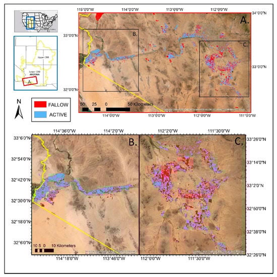
Figure 1.
The study regions in 2017 (A), including the lower Colorado river planning (LCRP) area (B), and the Pinal and Phoenix active management areas (PPAMA) (C). Base map shows the 2017 fallow-land algorithm based on neighborhood and temporal anomalies (FANTA) active (blue) and fallow (red) cropland classification. Inset map in upper-left outlines in yellow the upper and lower Colorado River Basin (CRB) and in red the region of interest for this study.
2.2. Satellite Data
An 8-day, 30-m normalized difference vegetation index (NDVI) time series from 2001–2017 was developed based on a statistical fusion of 30-m Landsat (Collection 2) and 250-m MODIS (MOD09Q1.006) surface reflectance observations. Utilizing concurrent Landsat satellites enabled an 8-day Landsat surface reflectance time series, with the exception of year 2012, since both Landsat 5 and Landsat 8 were offline. The Google Earth Engine (GEE) cloud-computing platform [33] was used to access all available Landsat and MODIS surface reflectance observations for the full study period. The Landsat and MODIS bands largely overlap in their coverage of the near infrared and red portions of the electromagnetic spectrum and produce consistent and accurate estimates of NDVI [34,35].
The effects of cloud cover were minimized using the Landsat surface reflectance pixel quality assurance (pixel_qa) band. All pixels with high cloud confidence and/or classified as impacted by clouds or cloud shadow were filtered from the analysis and gap-filled. Additionally, any pixels lacking retrievals for Landsat NDVI calculations were also filtered from the analysis and gap-filled. All filtered or missing pixels were gap-filled utilizing the temporally-nearest (typically adjacent), high quality MODIS surface reflectance composite pixel weighted by the ratio of the observed coincident Landsat to MODIS NDVI. A readily available 30-m Landsat NDVI product was used to confirm the accuracy of our retrieval and in our examination of cropland productivity (iNDVI) [34]. From the filtered and gap-filled 30-m, 8-day NDVI, we further derived estimates of monthly minimum, maximum, and range of NDVI for each pixel for input into the FANTA fallow land identification algorithm.
2.3. FANTA Fallow Land Identification Algorithm
The fallow-land algorithm based on neighborhood and temporal anomalies (FANTA) was adapted to be driven by 30-m, Landsat-based NDVI estimates (Wallace et al., 2017). We first defined cultivated lands based on the 30-m spatial resolution cropland classification of the national land cover database (NLCD), which were available for years 2001, 2006, 2011 and 2016 [36,37,38]. The NLCD products were used as a mask of cultivated lands for the year they were released and the next four consecutive years until an updated NLCD product was released (e.g., 2001 NLCD was used as a cropland mask from 2001 to 2005). The NLCD products provide the best available characterization of cropland extent for the study region but do not distinguish between active and fallow croplands [36,37,38].
The FANTA algorithm uses monthly NDVI temporal and spatial anomalies to classify a given cropland pixel as either active or fallow, comparing each pixel to its historical values and to its neighboring cropland pixel values based on a series of logical statements (Equations (1)–(4)). We used a conservative approach such that if any two or more of the below logical statements were true, then the pixel was classified as “fallow” for a given month. Conversely, if three or more of the below logical statements were false, then the cropland pixel was classified as “active” for a given month (Figure 1). For more algorithm details, please refer to Wallace et al. (2017).
Statement 1. Identify low greenness anomalies relative to each pixel’s long-term characteristics (temporal anomaly):
where the monthly NDVI maximum of a given cropland pixel (NDVImax) subtracted by its long-term monthly mean NDVI maximum (T_NDVImax) is compared to three times the long-term monthly NDVI maximum standard deviation (T_NDVImax_stdv).
Statement 2. Identify low monthly greenness variation relative to each pixel’s long-term characteristics (temporal anomaly):
where the monthly NDVI range of a given cropland pixel (NDVIrange) subtracted by its long-term monthly mean NDVI range (T_NDVIrange) is compared to three times its long-term monthly NDVI range standard deviation (T_NDVIrange_stdv).
Statement 3. Identify low greenness anomalies relative to each pixel’s neighbors (spatial anomaly):
where the monthly NDVI maximum of a given cropland pixel (NDVImax) is compared to 0.8 times the monthly mean NDVI maximum for all cropland pixels in the full region (S_NDVImax).
Statement 4. Identify low monthly greenness variation relative to each pixel’s neighbors (spatial anomaly):
where the monthly NDVI range of a given cropland pixel (NDVIrange) is compared to 0.8 times the monthly mean NDVI range for all cropland pixels in the full region (S_NDVIrange).
2.4. Ground Validation Data
Field data used for algorithm validation were collected by USGS personnel in 2014 in the PPAMA and 2017 in the LCRP. Over 5000 sites were visited, guided by preliminary analyses of the NLCD cropland data layer and NDVI status. Each field subplot within a greater field plot was treated as a vector polygon that was then categorized as either fallow or as the specific crop type if actively planted. A critical challenge of monitoring fallows lands is that they can look very different depending on management. For instance, fallow land maintained for future crop production may remain free of vegetation (low NDVI). Conversely, abandoned fallow land may experience natural regrowth (relatively high NDVI). The field sites used in the regional validation of the Landsat FANTA algorithm for this work included a diverse selection of fallow lands to ensure our approach accurately captured the full range of fallow cropland states [18]. FANTA fallow/active cropland estimates were extracted for all validation polygons and used to generate key statistics including producer’s, user’s and overall accuracy estimates. We utilized 100 randomly selected points within each validation polygon that represented each crop field.
2.5. Ancillary Data and Statistical Analysis
We examined relationships of active cropland extent and iNDVI to both climatic and socioeconomic variables using standard linear regression analyses. Climatic variables included precipitation (PPT), temperature, potential evapotranspiration (PET), vapor pressure deficit (VPD) and aridity provided by or derived from the parameter-elevation regression on independent slopes model (PRISM) products [39]. We calculated monthly estimates of PET using the FAO-56 Penman-Monteith method and aridity as the ratio between PPT and PET [40,41,42]. To account for the distinct summer and winter growing seasons characteristic of the regional hydroclimate, all meteorological and NDVI data were annually summarized for both the warm (DOY 97-273) and cool (DOY 273-97) seasons (Table S1). Socioeconomic data included Arizona crop market value data from the United States Department of Agriculture (USDA) National Agricultural Statistics Service (NASS) annual statistical bulletin [43]. Market value can be directly related to the supply of and demand for crop production, and these valuations can influence management decisions at a farm level [4]. We evaluated the influence of crop price on farm-level decision making by calculating the correlation between: (1) crop market value and cropland extent and (2) crop market value and active cropland productivity (e.g., iNDVI) [44]. All statistical analyses were conducted in the R statistical computing environment [45].
3. Results
3.1. Classification Performance
Based on ground observations collected in 2014 and 2017, we found overall classification accuracies of 88.9% and 87.2% for the LCRP and PPAMA, respectively (Figure 2; Tables S2 and S3). The LCRP had a user’s accuracy of 98.1% and a producer’s accuracy of 78.2% for active cropland, and a user’s accuracy of 83.3% and a producer’s accuracy of 98.6% for fallow cropland. PPAMA had a user’s accuracy of 90.4% and a producer’s accuracy of 91.0% for active cropland, and a user’s accuracy of 80.1% and a producer’s accuracy of 78.9% for fallow cropland. We note that cases of mixed active/fallow cropland within a single land parcel were a source of uncertainty in the ground observations that likely contributed to apparent reductions in model performance (Figure 2).
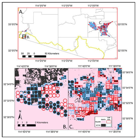
Figure 2.
Classification of fallow and active cropland extent for all USGS in situ observations (A); an example region within LCRP in 2014 (overall accuracy: 88.9%) (B); and an example region within PPAMA in 2017 (overall accuracy: 87.2%) (C). In situ observations of fallow (red) and active (light blue) cropland areas are shown as vector outlines, whereas FANTA estimates of fallow (pink) and active (black) are shown on the base map.
3.2. Active Cropland Extent and Productivity Trends
The LCRP, an area of senior water rights, consistently had a higher percentage of land that remained in active production (69.5% of croplands remained active for 15 or more years of the 17-year study period) relative to the PPAMA, an area of junior water rights (24.7% croplands remained active for 15 or more years of the 17-year study period) (Figure 3). The LCRP on average maintained 89.0% ± 1.6% of total cropland area in active production in any given year, whereas the PPAMA on average maintained 80.3% ± 2.4% of total cropland area in active production in any given year (Figure 4 and Figure S2). The LCRP active cropland extent decreased with increasing cool-season average vapor pressure deficit (R = −0.52, p < 0.01); whereas active cropland extent of the PPAMA increased with cool-season average aridity (PPT/PET) (R = 0.46, p < 0.05) (Figure 4, Tables S4 and S5). Active cropland productivity (i.e., iNDVI) for both regions was found to be highly sensitive to climate factors: active cropland productivity of the LCRP increased with cool-season average vapor pressure deficit (R = 0.72, p < 0.01), while active cropland productivity of the PPAMA increased with warm-season average aridity (PPT/PET) (R = 0.42, p < 0.05) (Figure 4, Tables S6 and S7).
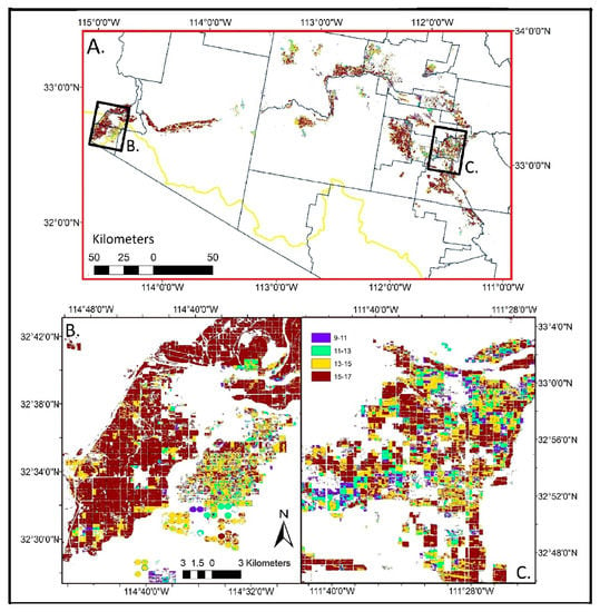
Figure 3.
Total number of years croplands remained in active production for the full LCRP and PPAMA study areas (A); an example region within LCRP (B); and an example region within PPAMA (C).
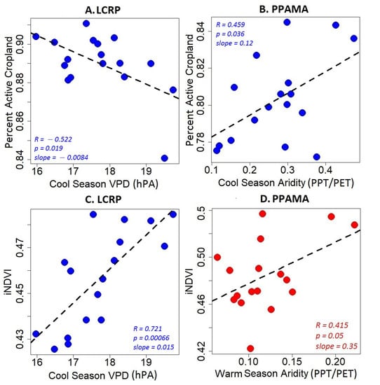
Figure 4.
The relationship between key climate factors and active cropland extent and productivity (iNDVI) from 2001 to 2017. LCRP active cropland extent (A) and iNDVI (C) were most sensitive to cool-season vapor pressure deficit, whereas PPAMA active cropland extent was most sensitive to mean cool-season aridity (B) and PPAMA cropland iNDVI was most sensitive to mean warm-season aridity (D). Each point indicates an annual mean estimate from 2001 to 2017. Dashed lines show the linear regression fit of all significant (p < 0.05) relationships. Blue signifies a relationship with cool-season climate variable while red represents a relationship with warm-season climate variable.
3.3. Active Cropland Extent, Productivity and Market Value
We evaluated the influence of crop price on farm-level decision making by calculating correlations between active cropland extent and productivity in years when market values are high (greater than the median value) versus years when they are low (less than the median value) [44]. For the PPAMA, a region of junior water rights, cropland extent and productivity were more positively correlated with cool-season aridity (PPT/PET) (R = 0.74, p < 0.01) and warm-season aridity (PPT/PET) (R = 0.62, p < 0.05), respectively, during periods of relatively low crop market value (Figure 5). For the LCRP, a region of senior water rights, cropland productivity was more positively correlated with cool-season vapor pressure deficit (R = 0.79, p < 0.01) during periods of relatively low crop market value, but differences between low and high market value years were not as great as in the PPAMA (Figure S3).
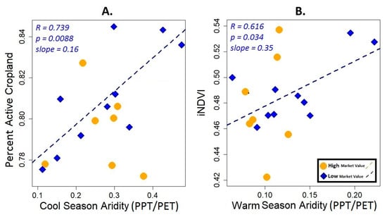
Figure 5.
The role of crop market value in the coupling of active cropland extent and active cropland productivity (iNDVI) to climate. PPAMA active cropland extent (A) and iNDVI (B) were most sensitive to mean cool season aridity during years of low market value (blue diamonds). Dashed lines show the linear regression fit of the low-market value relationships, which are significant (p < 0.05); Correlations and slopes are reported in the plot.
4. Discussion
Our analysis revealed that active cropland extent and productivity were dynamic and correlated with climate and socioeconomic factors. We found clear differences between our two regions of study: the lower Colorado River planning (LCRP) area, an area of cool-season cropping and senior water rights, and the Pinal and Phoenix active management areas (PPAMA), an area of warm-season cropping and junior water rights. The LCRP maintained a relatively high overall active cropland extent with low interannual variability, while the PPAMA maintained a lower mean active cropland extent with higher interannual variability (Figure 3 and Figure 4). This difference between regions is potentially driven by their similar dependence on water resources, which are not equally available due to hierarchical water rights.
For instance, the LCRP receives less mean annual precipitation (108.1 mm year−1), yet active cropland extent was relatively high and less sensitive to water constraints (Figure 4 and Figures S1–S3, Table S3), and cropland productivity (iNDVI) was even positively correlated with VPD. Conversely, the PPAMA receives more annual precipitation (270.7 mm year−1 on average), yet active cropland extent was lower than in the LCRP and was more sensitive to cool-season aridity (PPT/PET) (Figure 4 and Figures S1 and S2, Table S5). The difference in sensitivities suggests that despite very low average annual rainfall, senior water rights status of the LCRP provided more reliable access to Colorado River water resources, enabling minimal change in active cropland extent and productivity even in low precipitation years. The PPAMA sensitivity to cool-season aridity (PPT/PET), even though it is a warm season cropping region, could be explained by the influence of cool season weather on farmer decision making in a region with junior water rights. Farmers in the PPAMA may be more likely to decrease their cropland extent and experience decreases in overall productivity if there was a drier winter [46,47,48]. We note that the difference in growing season timing for the two regions is another confounding factor that could explain differences in sensitivity to climate (Table S1).
We also found evidence that crop market values influenced the coupling of active cropland extent and productivity to climate. For the PPAMA in particular, crop market value appeared to mediate the sensitivity of active cropland extent and productivity to moisture availability. For instance, when crop market value was low, PPAMA active crop extent and productivity were strongly correlated with cool- and warm-season aridity (Figure 5). One explanation for this trend could be that during low commodity price years farmers may be deciding the extent and intensity of irrigation based on water resource availability. Alternatively, during high commodity price years farmers may be maximizing the extent and intensity of irrigation even during drought years, such that crop productivity becomes insensitive to climate. The LCRP showed similar evidence of higher climate sensitivity of crop productivity during low market value years (Figure S3). This finding is in contrast to Deines et al. (2017), who found higher climate sensitivity of crop production in the US Northern High Plains during high commodity price year due to incentives for cropland expansion. These contrasting results demonstrate key regional differences in cropland management strategies and highlight the need for high spatiotemporal resolution analyses spanning climatic gradients to better understand and optimize water resource consumption across water-limited agricultural regions.
Overall, the proportion of active cropland extent varied interannually in response to both climatic conditions (e.g., drought) and socioeconomic factors (e.g., market values), and thus accounting for these factors and their interactions is critical to our understanding of future food and water security. We present an improved framework for active/fallow cropland mapping by integrating a cutting-edge fallow land mapping algorithm (FANTA) with GEE cloud computing, enabling the rapid processing of large volumes of the best-available long-term satellite observations. Next steps of this work include the integration of long-term records of land surface temperature (LST) derived from Landsat thermal bands, which when combined with other ancillary data including NDVI, could be used to track daily crop water use and status [49,50,51].
5. Conclusions
We assessed agricultural fallowing dynamics and crop productivity within the lower Colorado River Basin using the FANTA model in the Google Earth Engine. The FANTA model, based on greenness anomalies relative to historical patterns and neighboring pixels, produced accurate maps of active versus fallow agricultural extents in both study areas (LCRP and PPAMA). Our approach is self-calibrating based on simple inputs and spatiotemporal statistical analysis of greenness, and it produces annual spatially explicit fallow and active crop extent maps that provide consistent tracking of irrigation, which can supplement or support current cropland classifications for both scientific and managerial applications. Our products utilize high resolution datasets that can be applied to finer spatial scale management areas. Our analysis revealed long-term temporal dynamics in active cropland extent and productivity that were strongly correlated with climate factors. We found that the LCRP, a region of winter cropping and senior water rights, experienced relatively reduced sensitivity to water availability: annual fallow and active cropland extent remained relatively stable, while active cropland productivity was even positively correlated with cool-season vapor pressure deficit. By contrast, the PPAMA, a region of summer cropping and junior water rights, showed evidence of significant sensitivity to water availability: annual fallow and active cropland extent was positively correlated with cool-season aridity (PPT/PET), and active cropland productivity was positively correlated to warm-season aridity (PPT/PET). We also found that cropland productivity in the PPAMA was more sensitive to climate constraints when crop prices were relatively low, potentially due to the influence of market value on management decisions. Our approach, due to the relative simplicity of its inputs and processing, is transferable to other regions, allowing high spatiotemporal resolution mapping of agricultural dynamics that can provide valuable real-time information for research, land management and evidence-based decision-making.
Supplementary Materials
The following are available online at https://www.mdpi.com/article/10.3390/rs13091659/s1, Figures S1–S3, Tables S1–S7.
Author Contributions
Conceptualization, C.L.N. and W.K.S.; Methodology, C.L.N., J.R.R., C.S.A.W., W.J.D.v.L. and W.K.S.; Formal analysis, C.L.N., M.P.D., J.R.R. and D.Y.; writing—original draft preparation, C.L.N., W.K.S. and M.P.D.; writing—revisions, C.L.N., W.K.S., M.P.D., D.Y., C.S.A.W., J.R.R., S.M.M. and W.J.D.v.L. All authors have read and agreed to the published version of the manuscript.
Funding
We acknowledge support for this work provided by the Strategic Environmental Research and Development Program (SERDP; project number RC18-1322), the United States Department of Agriculture (USDA; cooperative agreement numbers 58-3050-9-013 and 58-2022-8-010), and the University of Arizona Earth Dynamics Observatory, funded by the office of Research, Innovation & Impact.
Data Availability Statement
Landsat (Collection 2) and MODIS (MOD09Q1.006) surface reflectance observations use in this study are available through the Google Earth Engine cloud computing platform (https://earthengine.google.com/ accessed on 15 January 2018). The Landsat NDVI product used in this study is available through the Numerical Terradynamic Simulation Group at the University of Montana (https://www.ntsg.umt.edu/project/landsat/ accessed on 15 January 2018). Gridded climate data used in this study are available from the PRISM Climate Group at Oregon State University (http://prism.oregonstate.edu accessed on 15 January 2018). Cropland classification data used in this study are available through the National Land Cover Database (available at: https://www.mrlc.gov/ accessed on 15 January 2018). FANTA active and fallow cropland extent estimated produced by this study are available at https://wkolby.org/data-code/ accessed on 15 January 2018.
Acknowledgments
We thank Nathaniel Robinson and Brady Allred for producing and providing key data used in this analysis. We also thank the PRISM Climate Group at Oregon State University and the producers of the National Land Cover Database. Finally, we acknowledge the Google Earth Engine cloud computing platform, without which this research would not have been possible. Any use of trade, product, or firm names in this paper is for descriptive purposes only and does not imply endorsement by the U.S. Government.
Conflicts of Interest
The authors declare no conflict of interest.
References
- Döll, P.; Siebert, S. Global modeling of irrigation water requirements. Water Resour. Res. 2002, 38, 8-1–8-10. [Google Scholar] [CrossRef]
- Siebert, S.; Döll, P. Quantifying blue and green virtual water contents in global crop production as well as potential production losses without irrigation. J. Hydrol. 2010, 384, 198–217. [Google Scholar] [CrossRef]
- McCabe, G.J.; Wolock, D.M. Warming may create substantial water supply shortages in the Colorado River basin. Geophys. Res. Lett. 2007, 34, L22708. [Google Scholar] [CrossRef]
- Mueller, N.D.; Gerber, J.S.; Johnston, M.; Ray, D.K.; Ramankutty, N.; Foley, J.A. Closing yield gaps through nutrient and water management. Nature 2012, 490, 254–257. [Google Scholar] [CrossRef]
- Rodell, M.; Famiglietti, J.S.; Wiese, D.N.; Reager, J.T.; Beaudoing, H.K.; Landerer, F.W.; Lo, M.H. Emerging trends in global freshwater availability. Nature 2018, 557, 651–659. [Google Scholar] [CrossRef] [PubMed]
- Ray, D.K.; Mueller, N.D.; West, P.C.; Foley, J.A. Yield trends are insufficient to double global crop production by 2050. PLoS ONE 2013, 8, e66428. [Google Scholar] [CrossRef]
- Milly, P.C.; Dunne, K.A. Potential evapotranspiration and continental drying. Nat. Clim. Chang. 2016, 6, 946–949. [Google Scholar] [CrossRef]
- Zhang, F.; Biederman, J.A.; Dannenberg, M.P.; Yan, D.; Reed, S.C.; Smith, W.K. Five Decades of Observed Daily Precipitation Reveal Longer and More Variable Drought Events Across Much of the Western United States. Geophys. Res. Lett. 2021, 48. [Google Scholar] [CrossRef]
- McCabe, G.J.; Wolock, D.M.; Pederson, G.T.; Woodhouse, C.A.; McAfee, S. Evidence that recent warming is reducing upper Colorado River flows. Earth Interact. 2017, 21, 1–14. [Google Scholar] [CrossRef]
- Udall, B.; Overpeck, J. The twenty-first century Colorado River hot drought and implications for the future. Water Resour. Res. 2017, 53, 2404–2418. [Google Scholar] [CrossRef]
- Woodhouse, C.A.; Pederson, G.T. Investigating runoff efficiency in upper Colorado River streamflow over past centuries. Water Resour. Res. 2018, 54, 286–300. [Google Scholar] [CrossRef]
- Deines, J.M.; Kendall, A.D.; Hyndman, D.W. Annual irrigation dynamics in the US northern high plains derived from Landsat satellite data. Geophys. Res. Lett. 2017, 44, 9350–9360. [Google Scholar] [CrossRef]
- Brown, J.F.; Pervez, M.S. Merging remote sensing data and national agricultural statistics to model change in irrigated agriculture. Agric. Syst. 2014, 127, 28–40. [Google Scholar] [CrossRef]
- Ozdogan, M.; Gutman, G. A new methodology to map irrigated areas using multi-temporal MODIS and ancillary data: An application example in the continental US. Remote Sens. Environ. 2008, 112, 3520–3537. [Google Scholar] [CrossRef]
- Wisser, D.; Frolking, S.; Douglas, E.M.; Fekete, B.M.; Vörösmarty, C.J.; Schumann, A.H. Global irrigation water demand: Variability and uncertainties arising from agricultural and climate data sets. Geophys. Res. Lett. 2008, 35. [Google Scholar] [CrossRef]
- Bradford, J.B.; Schlaepfer, D.R.; Lauenroth, W.K.; Yackulic, C.B.; Duniway, M.; Hall, S.; Jia, G.; Jamiyansharav, K.; Munson, S.M.; Wilson, S.D.; et al. Future soil moisture and temperature extremes imply expanding suitability for rainfed agriculture in temperate drylands. Sci. Rep. 2017, 7, 1–11. [Google Scholar] [CrossRef]
- Shivers, S.; Roberts, D.; McFadden, J.; Tague, C. Using Imaging Spectrometry to Study Changes in Crop Area in California’s Central Valley during Drought. Remote Sens. 2018, 10, 1556. [Google Scholar] [CrossRef]
- Wallace, C.S.; Thenkabail, P.; Rodriguez, J.R.; Brown, M.K. Fallow-land Algorithm based on Neighborhood and Temporal Anomalies (FANTA) to map planted versus fallowed croplands using MODIS data to assist in drought studies leading to water and food security assessments. Gisci. Remote Sens. 2017, 54, 258–282. [Google Scholar] [CrossRef]
- Richter, B.D.; Bartak, D.; Caldwell, P.; Davis, K.F.; Debaere, P.; Hoekstra, A.Y.; Li, T.; Marston, L.; McManamay, R.; Mekonnen, M.M.; et al. Water scarcity and fish imperilment driven by beef production. Nat. Sustain. 2020, 3, 319–328. [Google Scholar] [CrossRef]
- Anderson, J.R. A Land Use and Land Cover Classification System for Use with Remote Sensor Data; US Government Printing Office: Washington, DC, USA, 1976; Volume 964.
- Galvão, L.S.; Epiphanio, J.C.N.; Breunig, F.M.; Formaggio, A.R. Crop type discrimination using hyperspectral data. In Hyperspectral Remote Sensing of Vegetation; Thenkabail, P.S., Lyon, J.G., Huete, A., Eds.; CRC Press: Boca Raton, FL, USA, 2011; pp. 397–421. [Google Scholar]
- Acker, T.L.; Atwater, C.; Smith, D.H. Energy inefficiency in industrial agriculture: You are what you eat. Energy Sources Part B Econ. Plan. Policy 2013, 8, 420–430. [Google Scholar] [CrossRef]
- Bickel, A.K.; Duval, D.; Frisvold, G. Contribution of On-Farm Agriculture and Agribusiness to the Pinal County Economy; University of Arizona, Cooperative Extension: Tucson, AZ, USA, 2018. [Google Scholar]
- Bealmear, S.R.; Nolte, K.D. Planting and Harvesting Calendar for Gardeners in Yuma County; University of Arizona: Tuscon, AZ, USA, 2014. [Google Scholar]
- Lahmers, T.; Eden, S. Water and Irrigated Agriculture in Arizona; Arroyo, University of Arizona, Water Resources Research Center: Tucson, AZ, USA, 2018. [Google Scholar]
- Noble, W. A Case Study in Efficiency-Agriculture and Water Use in the Yuma, Arizona Area. Yuma County Agriculture Water Coalition. 2015. Available online: https://www.agwateryuma.com (accessed on 4 April 2020).
- Hanemann, W.M. The Central Arizona Project, Working Paper No. 937; Division of Agricultural and Natural Resources, University of California-Berkeley: Berkeley, CA, USA, 2002. [Google Scholar]
- Aggarwal, R.M.; Guhathakurta, S.; Grossman, C.S.; Lathey, V. How do the variations in urban heat islands in space and time influence household water use? The case of Phoenix, Arizona. Water Resour. Res. 2012, 48, W06578. [Google Scholar] [CrossRef]
- York, A.M.; Eakin, H.; Bausch, J.C.; Smith-Heisters, S.; Anderies, J.M.; Aggarwal, R.; Leonard, B.; Wright, K. Agricultural water governance in the desert: Shifting risks in central Arizona. Water Altern. 2020, 13, 418–445. [Google Scholar]
- Shupe, S.J.; Weatherford, G.D.; Checchio, E. Western water rights: The era of reallocation. Nat. Resour. J. 1989, 29, 413. [Google Scholar]
- Glennon, R.; Pearce, M.J. Transferring mainstem Colorado river water rights: The Arizona experience. Ariz. Law Rev. 2007, 49, 235. [Google Scholar]
- Sampson, D.A.; Cook, E.M.; Davidson, M.J.; Grimm, N.B.; Iwaniec, D.M. Simulating alternative sustainable water futures. Sustain. Sci. 2020, 15, 1199–1210. [Google Scholar] [CrossRef]
- Gorelick, N.; Hancher, M.; Dixon, M.; Ilyushchenko, S.; Thau, D.; Moore, R. Google Earth Engine: Planetary-scale geospatial analysis for everyone. Remote Sens. Environ. 2017, 202, 18–27. [Google Scholar] [CrossRef]
- Robinson, N.P.; Allred, B.W.; Jones, M.O.; Moreno, A.; Kimball, J.S.; Naugle, D.E.; Erickson, T.A.; Richardson, A.D. A dynamic Landsat derived normalized difference vegetation index (NDVI) product for the conterminous United States. Remote Sens. 2017, 9, 863. [Google Scholar] [CrossRef]
- Robinson, N.P.; Allred, B.W.; Smith, W.K.; Jones, M.O.; Moreno, A.; Erickson, T.A.; Naugle, D.E.; Running, S.W. Terrestrial primary production for the conterminous United States derived from Landsat 30 m and MODIS 250 m. Remote Sens. Ecol. Conserv. 2018, 4, 264–280. [Google Scholar] [CrossRef]
- Wickham, J.D.; Stehman, S.V.; Fry, J.A.; Smith, J.H.; Homer, C.G. Thematic accuracy of the NLCD 2001 land cover for the conterminous United States. Remote Sens. Environ. 2010, 114, 1286–1296. [Google Scholar] [CrossRef]
- Wickham, J.D.; Stehman, S.V.; Gass, L.; Dewitz, J.; Fry, J.A.; Wade, T.G. Accuracy assessment of NLCD 2006 land cover and impervious surface. Remote Sens. Environ. 2013, 130, 294–304. [Google Scholar] [CrossRef]
- Wickham, J.; Stehman, S.V.; Gass, L.; Dewitz, J.A.; Sorenson, D.G.; Granneman, B.J.; Poss, R.V.; Baer, L.A. Thematic accuracy assessment of the 2011 national land cover database (NLCD). Remote Sens. Environ. 2017, 191, 328–341. [Google Scholar] [CrossRef] [PubMed]
- PRISM Climate Group. Oregon State University. Available online: http://prism.oregonstate.edu (accessed on 4 February 2019).
- Daly, C.; Smith, J.I.; Olson, K.V. Mapping atmospheric moisture climatologies across the conterminous United States. PLoS ONE 2015, 10, e0141140. [Google Scholar] [CrossRef]
- Daly, C.; Halbleib, M.; Smith, J.I.; Gibson, W.P.; Doggett, M.K.; Taylor, G.H.; Curtis, J.; Pasteris, P.P. Physiographically sensitive mapping of climatological temperature and precipitation across the conterminous United States. Int. J. Climatol. 2008, 28, 2031–2064. [Google Scholar] [CrossRef]
- Allen, R.G.; Pereira, L.S.; Raes, D.; Smith, M. Crop Evapotranspiration-Guidelines for Computing Crop Water Requirements; FAO Irrigation and Drainage Paper 56; FAO: Rome, Italy, 1998; Volume 300, p. D05109. [Google Scholar]
- NASS (National Agricultural Statistics Service). Arizona Annual Statistics Bulletin; United States Department of Agriculture: Washington, DC, USA, 2019. Available online: https://www.nass.usda.gov/Statistics_by_State/Arizona/Publications/Annual_Statistical_Bulletin/index.php (accessed on 4 February 2019).
- Bontkes, T.S.; van Keulen, H. Modelling the dynamics of agricultural development at farm and regional level. Agric. Syst. 2003, 76, 379–396. [Google Scholar] [CrossRef]
- R Core Team. R: A Language and Environment for Statistical Computing; R Foundation for Statistical Computing: Vienna, Austria, 2020. [Google Scholar]
- Tabari, H.; Aghajanloo, M.B. Temporal pattern of aridity index in Iran with considering precipitation and evapotranspiration trends. Int. J. Climatol. 2013, 33, 396–409. [Google Scholar] [CrossRef]
- Deschênes, O.; Greenstone, M. The economic impacts of climate change: Evidence from agricultural output and random fluctuations in weather: Reply. Am. Econ. Rev. 2012, 102, 3761–3773. [Google Scholar] [CrossRef]
- Wu, D.; Zhao, X.; Liang, S.; Zhou, T.; Huang, K.; Tang, B.; Zhao, W. Time-lag effects of global vegetation responses to climate change. Glob. Chang. Biol. 2015, 21, 3520–3531. [Google Scholar] [CrossRef]
- Schnebele, E.; Tanyu, B.F.; Cervone, G.; Waters, N. Review of remote sensing methodologies for pavement management and assessment. Eur. Transp. Res. Rev. 2015, 7, 1–19. [Google Scholar] [CrossRef]
- Smith, W.K.; Dannenberg, M.P.; Yan, D.; Herrmann, S.; Barnes, M.L.; Barron-Gafford, G.A.; Biederman, J.A.; Ferrenberg, S.; Fox, A.M.; Hudson, A.; et al. Remote sensing of dryland ecosystem structure and function: Progress, challenges, and opportunities. Remote Sens. Environ. 2019, 233, 111401. [Google Scholar] [CrossRef]
- Fisher, J.B.; Melton, F.; Middleton, E.; Hain, C.; Anderson, M. The future of evapotranspiration: Global requirements for ecosystem functioning, carbon and climate feedbacks, agricultural management, and water resources. Water Resour. Res. 2017, 53, 2618–2626. [Google Scholar] [CrossRef]


Publisher’s Note: MDPI stays neutral with regard to jurisdictional claims in published maps and institutional affiliations. |
© 2021 by the authors. Licensee MDPI, Basel, Switzerland. This article is an open access article distributed under the terms and conditions of the Creative Commons Attribution (CC BY) license (https://creativecommons.org/licenses/by/4.0/).