Estimating Processing Tomato Water Consumption, Leaf Area Index, and Height Using Sentinel-2 and VENµS Imagery

Kaplan, Gregoriy; Fine, Lior; Lukyanov, Victor; Manivasagam, V. S.; Malachy, Nitzan; Tanny, Josef; Rozenstein, Offer

doi:10.3390/rs13061046

Open AccessArticle

Estimating Processing Tomato Water Consumption, Leaf Area Index, and Height Using Sentinel-2 and VENµS Imagery

¹

Institute of Soil, Water and Environmental Sciences, Agricultural Research Organization, Rishon LeZion 7528809, Israel

²

Department of Soil and Water Sciences, Faculty of Agriculture, Food and Environment, The Hebrew University of Jerusalem, Rehovot 7628604, Israel

³

Amrita School of Agricultural Sciences, Amrita Vishwa Vidyapeetham, J. P. Nagar, Arasampalayam, Myleripalayam, Coimbatore 642 109, India

⁴

HIT–Holon Institute of Technology, Holon 5810001, Israel

^*

Author to whom correspondence should be addressed.

Remote Sens. 2021, 13(6), 1046; https://doi.org/10.3390/rs13061046

Submission received: 1 February 2021 / Revised: 27 February 2021 / Accepted: 6 March 2021 / Published: 10 March 2021

(This article belongs to the Section Satellite Missions for Earth and Planetary Exploration)

Download

Browse Figures

Versions Notes

Abstract

:

Crop monitoring throughout the growing season is key for optimized agricultural production. Satellite remote sensing is a useful tool for estimating crop variables, yet continuous high spatial resolution earth observations are often interrupted by clouds. This paper demonstrates overcoming this limitation by combining observations from two public-domain spaceborne optical sensors. Ground measurements were conducted in the Hula Valley, Israel, over four growing seasons to monitor the development of processing tomato. These measurements included continuous water consumption measurements using an eddy-covariance tower from which the crop coefficient (K_c) was calculated and measurements of Leaf Area Index (LAI) and crop height. Satellite imagery acquired by Sentinel-2 and VENµS was used to derive vegetation indices and model K_c, LAI, and crop height. The conjoint use of Sentinel-2 and VENµS imagery facilitated accurate estimation of K_c (R² = 0.82, RMSE = 0.09), LAI (R² = 0.79, RMSE = 1.2), and crop height (R² = 0.81, RMSE = 7 cm). Additionally, our empirical models for LAI estimation were found to perform better than the SNAP biophysical processor (R² = 0.53, RMSE = 2.3). Accordingly, Sentinel-2 and VENµS imagery was demonstrated to be a viable tool for agricultural monitoring.

Keywords:

Sentinel-2; VENµS; Eddy covariance; crop coefficient; LAI; vegetation indices

Graphical Abstract

1. Introduction

Agriculture accounts for 70% of global freshwater usage [1,2], and therefore, increasing the agricultural water-use efficiency will improve agricultural sustainability. Where water is a limited resource, optimal water management is vital for food security. Crop coefficient (K_c)-based estimation of crop water consumption is one of the most commonly used irrigation management methods [3,4]. K_c is defined as the ratio between the actual evapotranspiration from a crop field and the environmental evaporative demand [3]. One of K_c estimation’s most reliable sources is vegetation indices (VIs) derived from optical remote sensing [5,6,7,8,9,10,11,12,13,14]. Until recently, this method’s application was hampered by the insufficient amount of public domain imagery at a high revisit time with fine spatial resolution. Since 2017 the Sentinel-2 constellation consists of two satellites and serves as a reliable satellite imagery source with high spatial (10, 20, or 60 meters; depending on the band) and temporal resolution (5 days). Despite that, in cloudy regions, even such a high temporal resolution might not be sufficient [15]. For example, despite the Sentinel-2 five-day revisit time, no cloud-free images were acquired for one and a half months in February and March 2018 over one of our experimental sites in Israel. Optical imagery from one satellite system could supplement the imagery from another system to address this problem. Previous studies have analyzed the performance of such conjunction of imagery from different platforms, for example, Landsat-7 and Landsat-8 [16], MODIS and Landsat-8 [17], as well as Landsat-8 and Sentinel-2 [18,19,20,21], and finally, Landsat-7, Landsat-8, and Sentinel-2 combined [22]. Similarly, the present study exploits the possibility of conjoint use of imagery acquired by the Sentinel-2 and the new Vegetation and Environment monitoring on a New MicroSatellite (VENµS) satellite, which has similar spectral bands in the visual, near infrared spectral region, and a 5–10 m spatial resolution (depending on the Collection) as Sentinel-2 in addition to a very high temporal resolution of two days [23].

Tomatoes are grown in many regions around the world. Previously, several studies were devoted to estimating tomato K_c based on lysimeters [24,25] or eddy covariance measurements [26,27] without the correlation to the satellite remote sensing data. Another approach previously used a mechanistic crop model to derive the crop evapotranspiration and correlate it with optical remote sensing data. In this way, previous work [28] used the EPIC model [29], which, in turn, used variables derived from Sentinel-2 imagery.

Additionally, satellite imagery was previously used to estimate other vegetation variables such as LAI and height [11,30,31,32,33,34]. Much like with K_c, VIs are good surrogates for other crop variables since there are similarities in the temporal change dynamics of VIs with LAI and height [35,36]. LAI is a good proxy of the vegetation state [37,38,39] and a good yield predictor [40]. Similarly, vegetation height estimation is useful for crop management [41]. Therefore accurate estimations of LAI and height from satellite imagery are desired.

Recently, the use of machine learning algorithms has become widespread in remote sensing. In the present study, the LAI biophysical processor [42] implemented in the ESA SNAP (Sentinel Application Platform) 7.0 software (http://step.esa.int/main/download/snap-download/, accessed on 21 February 2021) was tested. The LAI biophysical processor is a "black-box" module developed for Sentinel-2 imagery that cannot currently be used with other imagery.

Therefore, this study’s overarching aim was to derive empirical models to estimate vegetation variables based on a combined time series of spaceborne optical imagery from VENµS and Sentinel-2 and field measurements. Specifically, the goal was to develop reliable K_c, LAI, and height estimation models for processing tomato based on Sentinel-2 and VENµS imagery.

2. Materials and Methods

2.1. Test Sites and Field Measurements

The field data used in this study were collected during four experiments in commercial processing tomato fields in the Hula Valley, Israel (Figure 1, Table 1). Two experiments took place in Gadash farm in 2018 and 2019, and two more experiments were conducted in Kibutz Gadot in 2019 and 2020. LAI was measured by a SunScan Canopy Analysis System–SS1 manufactured by Delta-T Company (Cambridge, UK) during the two experiments conducted in 2019 and one experiment conducted in 2020. The SunScan is a widely used, accurate, nondestructive LAI measurement system that was successfully employed in many previous studies [31,43,44]. Plant height was measured using a measuring tape during all four experiments conducted in 2018–2020. Each LAI and vegetation height value used in the empirical modelling presented here is an average value of at least 30 field measurements. Both LAI and vegetation height were measured throughout the growing seasons; therefore, they represent the typical range of these variables.

The number of satellite images used for the development of the various models was not uniform because each model was based on the period for which field measurements were available, and therefore, a different number of corresponding satellite images. For example, LAI could not be measured using the SunScan system when the plants were very small, while vegetation height was easily measured at any time. Accordingly, the LAI models were based on shorter time-spans and fewer images than height models.

Each processing tomato field consisted of ridges and furrows. The distance between the rows was 2 m. Even during the vegetation development peak, the plants did not cover the furrows completely; thus, some soil reflectance signal is mixed with vegetation over the entire growing season. This mix of soil and vegetation reflectance hinders the vegetation variables estimation using remote sensing [45]. The Sentinel-2 and VENµS spectral bands used to derive vegetation indices were averaged for an area corresponding with the eddy-covariance footprint. In-field paths and their surrounding area were masked out from analysis polygons to remove bare soil areas and avoid edge effects. These excluded areas consisted of roughly 20% of the overall polygon areas. Therefore, each analysis consisted of either two or four vegetated regions separated by the paths (Figure 1).

2.2. Agro-Meteorological Measurements

The reference evapotranspiration, ET₀, was calculated based on nearby meteorological stations according to the FAO56 Penman–Monteith method based on meteorological measurements of air temperature, relative humidity, wind speed, and solar irradiance [3]. The actual evapotranspiration (ET_c) was measured using eddy covariance systems [26]. Based on these two measurements, the crop coefficient, K_c, was calculated as: K_c = ET_c/ET₀. K_c is an important variable used to determine the irrigation dose [9]. The resulting K_c time series were smoothed using cubic or second-order splines.

2.3. Satellite Imagery

Sentinel-2 is an Earth observation mission and part of the European Space Agency (ESA) Copernicus program. It includes two satellites, each equipped with a Multi-Spectral Instrument (MSI), namely, Sentinel-2A (launched June 2015) and Sentinel-2B (launched March 2017). VENµS is a joint satellite mission of the Israeli and French space agencies (ISA and CNES) launched in August 2017. VENµS has a two-day revisit time over Israel and a multispectral camera with 12 narrow spectral bands in the range of 415–910 nm [46]. VENµS and Sentinel-2 produce 10 and 12-bit radiometric data, respectively. The radiometric correction procedure of VENµS imagery was updated in 2020. The imagery acquired before the update is known as Collection 1; the imagery acquired after the update is known as Collection 2. VENµS captures s imagery with a spatial resolution of 10 m. Sentinel-2 RGB and NIR bands also have a spatial resolution of 10 m, and other bands are coarser: narrow NIR, SWIR, and red edge bands, 20 m; coastal aerosol, water vapour, and SWIR-cirrus bands used mostly for atmospheric correction, 60 m. Atmospherically corrected reflectance products from both sensors were used in this analysis. Level-2 VENµS products, initially distributed at 10 m spatial resolution, were later distributed at a resolution of 5 m when an updated processing procedure was initiated in 2020. This product was used for the analysis of the 2020 experiment in Gadot. Sentinel-2 level-2A data were obtained from the ESA Copernicus Open Access Hub website (https://scihub.copernicus.eu/dhus/#/home, accessed on 21 February 2021). VENµS level-2 products were obtained from the Israel VENµS website maintained by Ben-Gurion University of the Negev (https://venus.bgu.ac.il/venus/, accessed on 21 February 2021). Table 2 lists the overlapping spectral bands of the Sentinel-2 and VENµS sensors used in this study to derive vegetation indices. The LAI and K_c estimation models were derived based on three seasons, and crop height models were based on four seasons. An inventory of the Sentinel-2 and VENµS images used in the present study can be found in Table 3, alongside the number of LAI and height measurements taken during each season and used for model derivation.

2.4. Vegetation Indices and Model Validation

All Sentinel-2 and VENµS bands were resampled to 10 m spatial resolution. After that, thirteen vegetation indices (Appendix A) were derived based on the Sentinel-2 and VENµS imagery, including transformed VENµS imagery that utilised a corrective transformation (Table 4) derived for collection 1 VENµS imagery [23]. Since the radiometric processing of VENµS was improved in collection 2, the applicability of the transformation functions to the re-calibrated VENµS imagery was studied by comparing the performance of models based on the imagery transformed for all seasons against the models based on transformed imagery for 2018–2019 seasons (collection 1) and not transformed for 2020 (collection 2). The performance of the former was found to be better than the latter. Therefore, the transformed VENµS imagery models were applied to all seasons. Overall, three types of tomato estimation models were derived: models based on Sentinel-2; models based on Sentinel-2/non-transformed VENµS; models based on the Sentinel-2/transformed VENµS imagery. Hereafter the combined Sentinel-2/transformed VENµS models will be referred to as S2/V_T, and combined Sentinel-2/non-transformed VENµS models will be referred to as S2/V_NT.

Linear regression models were derived for the time series of field-measured K_c, LAI, height, and each spectral index time series. Each model was based on all available field measurements of each vegetation variable collected during all seasons when the variable was measured. For every model, the R² and root mean square error (RMSE) values were calculated. RMSE was calculated for each model based on all available data and also for each field experiment separately. In addition to vegetation index-based models, an LAI estimation from the ESA SNAP 7.0 biophysical processor for Sentinel-2 imagery was also produced [42].

The S2/V_T and S2/V_NT models were compared, and the Steiger variation [47] of the two-tailed Fisher’s Z-score tests [48] was performed to determine whether the difference in the models’ R² is significant (α ≤ 0.05). The same test was also performed to determine whether the difference in R² of the LAI Biophyscal processor and DVI was significant.

The field-measured processing tomatoes LAI and height measured in Gadash 2019 and Gadot in 2019 and 2020 were used to calibrate prediction models for K_c, as was done previously [49].

3. Results

Figure 2 presents the experiments’ measured LAI and crop height, field measured K_c, the smoothed K_c, and the standard K_c table of the Israeli Extension Service. Figure 2A–D shows height values measured during four experiments and LAI values measured during three experiments. Figure 2E–G shows the three types of the aforementioned variations of the K_c associated with three experiments conducted in Israel. The standard K_c recommendation differs from the measured K_c values. Early in the season, during the crop vegetative development, the standard table recommendation is slightly higher than the measured water consumption. In Gadot 2019, the standard recommendation and measured water consumption are about the same at the peak. In Gadot 2020 and Gadash 2019, the standard recommendation’s peak is higher than the measured water consumption. However, from the mid-late season, the measured water consumption drops below the standard recommendation. Interestingly, in Gadash 2019, the crop height and LAI and the K_c were lower compared to the other seasons. Moreover, the changes in LAI and height in Gadash 2019 were different compared to other seasons. These discrepancies in behavior between tomato variables and differences in the variables’ values from season to season demonstrate the variance in crop development and water consumption between seasons. Therefore, real-time estimations of those variables are advantageous over the use of standard tables.

GEMI and WDVI were found to be the best VIs for the tomato K_c, crop height, and LAI estimation. These results repeated in all three types of models: Sentinel-2-based, S2/V_NT, and S2/V_T. Table 5, Table 6 and Table 7 show Sentinel-2, S2/V_NT, and S2/V_T-based K_c, crop height, and LAI estimation models based on the five best-performing VIs: DVI, GEMI, WDVI, SAVI, and MSAVI. The best combined Sentinel-2/VENµS models in the present study are presented in Figure 3. The data points in Figure 3 are not clustered by sensors or experiments, which is indicative of the models’ generality. Therefore, both sensors used in the study can be employed interchangeably. The tomato K_c, height, and LAI estimation models’ performance is based on eight other VIs (NDVI, MTCI, IPVI, IRECI, S2REP, REIP, GNDVI, and TNDVI), which can be found in Appendix B, Appendix C, Appendix D. Table 5 shows that the RMSE of LAI derived from the biophysical processor is higher and the R² is lower than VIs such as GEMI, DVI, WDVI, SAVI, and MSAVI. The biophysical processor’s R² was found significantly lower than the R² of DVI (p = 0.016). It was found that the majority of S2/V_T and S2/V_NT models do not present significant differences in performance and that the transformation of VENµS imagery is mostly beneficial for the red edge VIs such as MTCI and S2REP (Appendix E). Table 8 shows the difference in performance between S2/V_T models and S2/V_NT models of the best performing VIs (DVI, GEMI, WDVI, SAVI, and MSAVI). Appendix E shows the difference in performance between S2/V_T models and S2/V_NT models for eight additional VIs (NDVI, MTCI, IPVI, IRECI, S2REP, REIP, NDVI, and TNDVI).

Figure 4 shows data acquired during two experiments in 2019 and one experiment in 2020. Figure 4A shows LAI and height measurements (in dm; to fit them to the same Y-axis) recorded during three field campaigns in 2019 and 2020. Interestingly, in Gadot 2019, height continued to increase in the middle of the season, while LAI has already started to decrease. In the other fields measured in this study, LAI and height varied simultaneously. Figure 4B shows the smoothed measured K_c curve, the standard K_c table values provided by the Israeli Extension Service (IES), and the estimated K_c values based on the S2/V_NT GEMI model. The field measured K_c varied from season to season, and in Gadash 2019, the measured K_c showed the most considerable difference from the recommended curve, especially in the middle part of the season (approximately 60 days after planting). Moreover, the measured K_c increase, especially during experiments in 2019, does not match the timing of the K_c increase provided by the IES. This demonstrates the significance of using K_c values estimated for a specific field at a specific season for efficient irrigation. The low values of K_c, LAI, and height in Gadash 2019 might be explained by the high amount of weeds present in the field during the experiment.

The performance of processing tomato height and LAI-based K_c estimation models using field measurements is shown in Table 9.

4. Discussion

The field experiments conducted in Israel in 2018–2020 showed that K_c, LAI, and crop height in processing tomato differ from season to season but can be estimated correctly in near-real-time from satellite remote sensing imagery. Consequently, agricultural decisions, including the irrigation dose determination, can rely on remote sensing data rather than standard tabular recommendations until late in the season. During the last stage of the season, deficit irrigation is applied according to the percentage of ripe fruit (the ratio of red to green tomatoes on the plant) to delay ripening or expedite it according to the desired harvest schedule [50]. Thus, the irrigation dose at the end of the season cannot be estimated using the remote sensing approach described here.

The field-measured K_c in this study yielded high correlations with VIs from Sentinel-2 and VENµS. Consequently, this study paves the way for more precise K_c, LAI, and crop height estimations on a local and global scale based on the freely available optical satellite imagery. These crop variable estimations could be used for better irrigation and fertilization management [51], as well as for early detection of crop disease [52,53], waterlogging [54,55], pest management, and biological control [56].

This study’s most important result was the demonstration of effectively joining Sentinel-2, and VENµS imagery for agricultural monitoring suggested before the launch of those missions [38]. This was possible because of the close resemblance of Sentinel-2 and VENµS spectral response functions and a good radiometric and atmospheric correction. Application of corrective transformation functions [23] improved the performance of VIs based on the red edge bands (MTCI, S2REP, and REIP), while for the other VIs, the transformation was found unnecessary or provided only marginal performance improvement.

Many VIs showed good K_c estimation performance; the best performing K_c estimation was achieved with the GEMI S2/V_NT model (R² = 0.82, RMSE = 0.09). In an earlier study, a canopy cover-based K_c estimation model achieved R² = 0.96 [27]. In that study, the canopy cover was calculated using cameras installed in the field. Unlike this approach that relies on in-field sensors, the approach suggested in this paper, based on satellite remote sensing, facilitates the estimation of vegetation variables over more extensive areas at a low cost. This study shows that K_c estimation from optical satellite remote sensing can serve as a reliable source for irrigation decisions and potentially for other agricultural activities throughout the whole growing season of processing tomato. The best performing LAI estimation models showed promising results (S2/V_T WDVI LAI estimation model: R² = 0.79, RMSE = 1.2). This result agrees with a previous study that found WDVI, which takes soil reflectance into account, as a good indicator of LAI [57]. In comparison to the newly-obtained processing tomato LAI models, multi-crop models derived in previous studies demonstrated lower performance, e.g., R² = 0.62 [58], R² = 0.66 [59], R² = 0.72 [60]. A tomato LAI model from previous work [28] showed a lower coefficient of determination (R² = 0.69) and lower RMSE = 0.56 compared to this study. However, this model was based on only four days of field measurements. Moreover, that work [28] did not include LAI measurements in the final stage of a growing season, while the LAI models in the present study were based on three full growing seasons. Consequently, the processing tomato LAI estimation models developed in the present study are suitable for general use in precision agriculture applications throughout the growing season. Additionally to LAI estimation based upon the VIs, the performance of the SNAP biophysical processor LAI estimation algorithm was studied (R² = 0.53, RMSE = 2.3) and found to be significantly less accurate compared to the empirical model based on DVI, which was found to be the most accurate Sentinel-2-based VI for LAI estimation.

Similar to K_c and LAI estimation models, the tomato height estimation models were found to perform well throughout the processing tomato growing season. The S2/V_T WDVI-based height estimation model (R² = 0.81, RMSE = 7 cm) was found to be the best, and this approach shows great promise for agricultural crop monitoring. The obtained results confirmed the previously found conclusion that WDVI is a well-suited VI for crop LAI and height estimations [33].

K_c, LAI, and height estimation models based solely on Sentinel-2 data were as accurate as the combined Sentinel-2/VENµS models. Subsequently, a pooled time-series of imagery from both sensors increases the available satellite imagery’s temporal resolution. In cloudy regions, either sensor could fill gaps in the acquisitions of the other, and either sensor can efficiently monitor crop development when imagery from the other sensor is not available. For example, during both experiments in 2019, many VENµS images filled in a long gap in Sentinel-2 data in April–May, and one Sentinel-2 image filled a gap in VENµS images in May–June.

Additionally to the K_c estimation based on the remote sensing data, K_c estimation models based on the field measured LAI and height were derived. These models’ performance was similar to the remote sensing-based models and might be used on the local scale in the absence of remote sensing imagery. The K_c-height model is of particular interest from a practical viewpoint since farmers can easily and routinely take plant height measurements.

While this study provided useful results from thirteen VIs (including VIs based on the red edge bands and soil adjusted VIs) to estimate K_c, LAI, and height in the processing tomato using Sentinel-2 and VENµS imagery, there is merit in future studies on other crops. Future efforts could follow the procedure suggested in this paper to empirically calibrate and test prediction models for different indices and identify those that achieve the best performance. Studies based on two or more different sensors should make sure to perform a radiometric calibration between sensors.

5. Conclusions

This work demonstrates the conjoint use of Sentinel-2 and VENµS imagery for estimating K_c, LAI, and height of processing tomato. It was found that red edge VIs should be based on Sentinel-2 and transformed VENµS imagery. At the same time, other VIs can be derived directly from imagery obtained by both systems, and no corrective transformation is required to match the two sensors. In addition, models based solely on Sentinel-2 showed similar performance as the joint Sentinel-2 and VENµS imagery models. The K_c, LAI, and height estimation models derived empirically using field measurements show good performance and are ready for application. The LAI estimation performance from the SNAP biophysical processor was also studied and found inferior to the VI-based LAI estimation models. The irrigation in the early and middle parts of the processing tomato growing season can rely on remote sensing-based models rather than standard table values to best match the actual crop development and capture within-field variability.

Author Contributions

Conceptualization, O.R. and G.K.; methodology, G.K., J.T., and O.R., software, G.K., L.F., and V.L.; formal analysis, G.K.; investigation, G.K., J.T., and O.R.; fieldwork, G.K., V.L., L.F., V.S.M., N.M. and O.R.; writing—original draft preparation, G.K. and O.R.; writing—review and editing, G.K., O.R., V.S.M., J.T. and L.F.; visualization, G.K., O.R. and V.S.M.; supervision, J.T. and O.R.; project administration, J.T. and O.R.; funding acquisition, J.T. and O.R. All authors have read and agreed to the published version of the manuscript.

Funding

This research was funded by the Ministry of Science and Technology, Israel, under grant numbers 3-14559, 3-15605 and by the Chief Scientist of the Ministry of Agriculture under grant number 20-21-0006. Gregoriy Kaplan was supported by an absorption grant for new immigrant scientists provided by the Israeli Ministry of Immigrant Absorption. V. S. Manivasagam was supported by the ARO Postdoctoral Fellowship Program from the Agriculture Research Organization, Volcani Center, Israel.

Data Availability Statement

Weather data can be accessed on https://meteo.co.il/. Sentinel-2 level-2A data were obtained from the ESA Copernicus Open Access Hub website (https://scihub.copernicus.eu/dhus/#/home). VENµS level-2 products were obtained from the Israel VENµS website maintained by Ben-Gurion University of the Negev (https://venus.bgu.ac.il/venus/).

Acknowledgments

We thank the growers in Gadash farm and Kibbutz Gadot.

Conflicts of Interest

The authors declare no conflict of interest.

Appendix A

Table A1. Vegetation indices used in the present study.

	Index Name	Formula	Reference
1	Normalised Difference Vegetation Index (NDVI)	$\frac{(N I R - R E D)}{(N I R + R E D)}$	[61]
2	Global Environmental Monitoring Index (GEMI)	$ή * (1 - 0.25 * ή) - \frac{[(R E D - 0.125)]}{(1 - R E D)}$ where ή = $\frac{[2 * (N I R_{2} - R E D_{2}) + 1.5 * N I R + 0.5 * R E D]}{(N I R + R E D + 0.5)}$	[62]
3	Weighted Difference Vegetation Index (WDVI)	$N I R - S * R E D$ where: S is the slope of the soil line.	[63]
4	Green Normalized Difference Vegetation Index (GNDVI)	$\frac{(N I R - G R E E N)}{(N I R + G R E E N)}$	[64]
5	Modified Soil Adjusted Vegetation Index (MSAVI)	$\frac{(N I R - R E D) * (1 + L)}{(N I R + R E D + L)}$ where: L = $1 - \frac{2 * s * (N I R - R E D) * (N I R - s * R E D)}{(N I R + R E D)}$ where s is the slope of the soil line from a plot of red versus near infrared brightness values	[65]
6	Difference Vegetation Index (DVI)	$N I R - R E D$	[61]
7	MERIS terrestrial chlorophyll index (MTCI)	$\frac{(N I R - R E)}{(R E - R E D)}$	[66]
8	Infrared Percentage Vegetation Index (IPVI)	$\frac{N I R}{(N I R + R E D)}$	[67]
9	Inverted Red Edge Chlorophyll Index (IRECI)	$\frac{(N I R - R E D)}{(R E 1 / R E 2)}$	[68]
10	Sentinel-2 Red Edge Position (S2REP)	$705 + 35 * \frac{(\frac{p 783 + p 665}{2}) - p 705}{p 740 - p 705}$	[68]
11	Red Edge In-flection Point (REIP)	$700 + 40 * \frac{\frac{p 670 + p 780}{2} - p 700}{p 740 - p 700}$	[69]
12	Soil Adjusted Vegetation Index (SAVI)	$\frac{(N I R - R E D)}{(N I R + R E D + L)} * (1 + L)$	[70]
13	Transformed Normalized Difference Vegetation Index (TNDVI)	$\sqrt[]{(\frac{(N I R - R E D)}{(N I R + R E D)} + 0.5)}$	[71]

Appendix B

Table A2. Performance statistics of newly developed Sentinel-2-based LAI, Height, K_c models, and the performance of the SNAP biophysical processor LAI estimation algorithm. Performance statistics of better performing VIs can be found in Table 5.

Vegetation Index	Dataset	LAI		Height		K_c
Vegetation Index	Dataset	R²	RMSE	R²	RMSE (cm)	R²	RMSE
NDVI	Sentinel-2 Gadash 2018				9
	Sentinel-2 Gadash 2019		1.5		11		0.0919
	Sentinel-2 Gadot 2019		1.5		5		0.0961
	Sentinel-2 Gadot 2020		1.2		9		0.0558
	All seasons	0.6594	1.4	0.6387	9	0.7524	0.0826
MTCI	Sentinel-2 Gadash 2018				12
	Sentinel-2 Gadash 2019		2.0		11		0.1608
	Sentinel-2 Gadot 2019		2.6		11		0.1804
	Sentinel-2 Gadot 2020		2.1		8		0.0724
	All seasons	0.16	2.3	0.5216	10	0.2653	0.1433
IPVI	Sentinel-2 Gadash 2018				9
	Sentinel-2 Gadash 2019		1.5		11		0.0919
	Sentinel-2 Gadot 2019		1.5		5		0.0961
	Sentinel-2 Gadot 2020		1.2		9		0.0558
	All seasons	0.6594	1.4	0.6387	9	0.7524	0.0826
IRECI	Sentinel-2 Gadash 2018				9
	Sentinel-2 Gadash 2019		1.1		8		0.1084
	Sentinel-2 Gadot 2019		1.7		6		0.1646
	Sentinel-2 Gadot 2020		1.2		6		0.0674
	All seasons	0.6927	1.4	0.7688	7	0.4636	0.1233
S2REP	Sentinel-2 Gadash 2018				11
	Sentinel-2 Gadash 2019		2.1		12		0.1619
	Sentinel-2 Gadot 2019		2.5		10		0.1750
	Sentinel-2 Gadot 2020		2.1		9		0.0730
	All seasons	0.1642	2.3	0.5359	10	0.2893	0.1411
REIP	Sentinel-2 Gadash 2018				16
	Sentinel-2 Gadash 2019		2.1		14		0.1619
	Sentinel-2 Gadot 2019		2.5		8		0.1750
	Sentinel-2 Gadot 2020		2.1		10		0.0730
	All seasons	0.1642	2.3	0.3176	12	0.2893	0.1411
GNDVI	Sentinel-2 Gadash 2018				10
	Sentinel-2 Gadash 2019		1.6		12		0.1138
	Sentinel-2 Gadot 2019		1.6		6		0.1287
	Sentinel-2 Gadot 2020		1.4		9		0.0660
	All seasons	0.6093	1.5	0.6314	9	0.6048	0.1059
TNDVI	Sentinel-2 Gadash 2018				9
	Sentinel-2 Gadash 2019		1.6		12		0.0955
	Sentinel-2 Gadot 2019		1.5		6		0.0931
	Sentinel-2 Gadot 2020		1.3		9		0.0538
	All seasons	0.6456	1.5	0.6222	9	0.7572	0.0818

Appendix C

Table A3. Performance statistics of S2/V_NT-based LAI, Height, K_c models. Performance statistics of better performing VIs can be found in Table 6.

Vegetation Index	Dataset	LAI		Height		K_c
Vegetation Index	Dataset	R²	RMSE	R²	RMSE (cm)	R²	RMSE
NDVI	Sentinel-2 Gadash 2018				9
	VENµS Gadash 2018				9
	Sentinel-2 Gadash 2019		1.5		11		0.0939
	VENµS Gadash 2019		1.0		10		0.0718
	Sentinel-2 Gadot 2019		1.5		5		0.0887
	VENµS Gadot 2019		1.6		8		0.1115
	Sentinel-2 Gadot 2020		1.2		9		0.0700
	VENµS Gadot 2020		1.2		8		0.0844
	All seasons	0.8099	1.4	0.6885	9	0.7009	0.0905
MTCI	Sentinel-2 Gadash 2018				17
	VENµS Gadash 2018				11
	Sentinel-2 Gadash 2019		1.6		6		0.1439
	VENµS Gadash 2019		2.1		13		0.1869
	Sentinel-2 Gadot 2019		2.8		14		0.2325
	VENµS Gadot 2019		2.8		10		0.1845
	Sentinel-2 Gadot 2020		2.4		10		0.0869
	VENµS Gadot 2020		2.1		11		0.1559
	All seasons	0.0804	2.4	0.4062	12	0.2945	0.1750
IPVI	Sentinel-2 Gadash 2018				9
	VENµS Gadash 2018				9
	Sentinel-2 Gadash 2019		1.5		11		0.0939
	VENµS Gadash 2019		1.0		10		0.0718
	Sentinel-2 Gadot 2019		1.5		5		0.0887
	VENµS Gadot 2019		1.6		8		0.1114
	Sentinel-2 Gadot 2020		1.2		9		0.0701
	VENµS Gadot 2020		1.2		8		0.0841
	All seasons	0.7012	1.4	0.687	9	0.8103	0.0904
IRECI	Sentinel-2 Gadash 2018				10
	VENµS Gadash 2018				9
	Sentinel-2 Gadash 2019		1.0		7		0.0964
	VENµS Gadash 2019		0.9		7		0.1378
	Sentinel-2 Gadot 2019		1.8		7		0.1753
	VENµS Gadot 2019		1.7		6		0.1605
	Sentinel-2 Gadot 2020		1.0		5		0.0670
	VENµS Gadot 2020		1.7		9		0.1493
	All seasons	0.661	1.5	0.7684	7	0.5179	0.1447
S2REP	Sentinel-2 Gadash 2018				12
	VENµS Gadash 2018				10
	Sentinel-2 Gadash 2019		1.9		9		0.1456
	VENµS Gadash 2019		2.0		11		0.1538
	Sentinel-2 Gadot 2019		2.8		15		0.2199
	VENµS Gadot 2019		2.7		9		0.1752
	Sentinel-2 Gadot 2020		2.1		8		0.0790
	VENµS Gadot 2020		2.0		10		0.1514
	All seasons	0.1541	2.3	0.5588	10	0.4066	0.1616
REIP	Sentinel-2 Gadash 2018				14
	VENµS Gadash 2018				13
	Sentinel-2 Gadash 2019		2.5		18		0.2019
	VENµS Gadash 2019		1.8		8		0.1307
	Sentinel-2 Gadot 2019		2.4		8		0.1611
	VENµS Gadot 2019		2.8		11		0.1940
	Sentinel-2 Gadot 2020		2.1		13		0.1398
	VENµS Gadot 2020		2.0		9		0.1235
	All seasons	0.1509	2.3	0.4815	11	0.4223	0.1591
GNDVI	Sentinel-2 Gadash 2018				11
	VENµS Gadash 2018				9
	Sentinel-2 Gadash 2019		1.3		10		0.0963
	VENµS Gadash 2019		1.0		9		0.0779
	Sentinel-2 Gadot 2019		1.9		7		0.1411
	VENµS Gadot 2019		1.7		7		0.1048
	Sentinel-2 Gadot 2020		1.3		8		0.0752
	VENµS Gadot 2020		1.5		8		0.1075
	All seasons	0.6477	1.5	0.6934	9	0.7631	0.1014
TNDVI	Sentinel-2 Gadash 2018				9
	VENµS Gadash 2018				9
	Sentinel-2 Gadash 2019		1.6		12		0.0992
	VENµS Gadash 2019		1.1		10		0.0711
	Sentinel-2 Gadot 2019		1.5		6		0.0849
	VENµS Gadot 2019		1.6		8		0.1101
	Sentinel-2 Gadot 2020		1.3		9		0.0675
	VENµS Gadot 2020		1.1		8		0.1006
	All seasons	0.6899	1.4	0.6706	9	0.7978	0.0934

Appendix D

Table A4. Performance statistics of S2/V_T-based LAI, Height, K_c. Performance statistics of better performing VIs can be found in Table 7.

Vegetation Index	Dataset	LAI		Height		K_c
Vegetation Index	Dataset	R²	RMSE	R²	RMSE (cm)	R²	RMSE
NDVI	Sentinel-2 Gadash 2018				7
	VENµS Gadash 2018				12
	Sentinel-2 Gadash 2019		2.0		14		0.1223
	VENµS Gadash 2019		1.0		9		0.0665
	Sentinel-2 Gadot 2019		1.2		5		0.0662
	VENµS Gadot 2019		2.0		10		0.1461
	Sentinel-2 Gadot 2020		1.4		10		0.0926
	VENµS Gadot 2020		1.2		8		0.0863
	All seasons	0.623	1.5	0.6156	10	0.743	0.1053
MTCI	Sentinel-2 Gadash 2018				12
	VENµS Gadash 2018				14
	Sentinel-2 Gadash 2019		2.1		12		0.1649
	VENµS Gadash 2019		1.5		6		0.1368
	Sentinel-2 Gadot 2019		2.6		10		0.1802
	VENµS Gadot 2019		2.7		11		0.1823
	Sentinel-2 Gadot 2020		2.0		9		0.0906
	VENµS Gadot 2020		2.0		12		0.1561
	All seasons	0.2094	2.2	0.5212	11	0.4222	0.1583
IPVI	Sentinel-2 Gadash 2018				7
	VENµS Gadash 2018				11
	Sentinel-2 Gadash 2019		2.1		14		0.1253
	VENµS Gadash 2019		0.7		7		0.0906
	Sentinel-2 Gadot 2019		1.2		5		0.0635
	VENµS Gadot 2019		1.9		9		0.1431
	Sentinel-2 Gadot 2020		1.5		10		0.0971
	VENµS Gadot 2020		1.2		8		0.0904
	All seasons	0.646	1.5	0.6454	9	0.7233	0.1092
IRECI	Sentinel-2 Gadash 2018				7
	VENµS Gadash 2018				11
	Sentinel-2 Gadash 2019		1.4		10		0.0916
	VENµS Gadash 2019		0.8		7		0.1394
	Sentinel-2 Gadot 2019		1.4		6		0.1527
	VENµS Gadot 2019		1.9		8		0.1713
	Sentinel-2 Gadot 2020		1.9		11		0.1588
	VENµS Gadot 2020		1.3		5		0.1125
	All seasons	0.6527	1.5	0.7349	8	0.5139	0.1453
S2REP	Sentinel-2 Gadash 2018				9
	VENµS Gadash 2018				12
	Sentinel-2 Gadash 2019		2.3		16		0.1905
	VENµS Gadash 2019		1.7		7		0.1186
	Sentinel-2 Gadot 2019		2.5		8		0.1636
	VENµS Gadot 2019		2.7		10		0.1556
	Sentinel-2 Gadot 2020		2.1		11		0.1208
	VENµS Gadot 2020		1.9		8		0.0978
	All seasons	0.1992	2.3	0.5893	10	0.5709	0.1366
REIP	Sentinel-2 Gadash 2018				11
	VENµS Gadash 2018				15
	Sentinel-2 Gadash 2019		2.8		22		0.2433
	VENµS Gadash 2019		1.6		7		0.1249
	Sentinel-2 Gadot 2019		2.4		10		0.1658
	VENµS Gadot 2019		2.8		11		0.1785
	Sentinel-2 Gadot 2020		2.3		14		0.1563
	VENµS Gadot 2020		2.1		9		0.0887
	All seasons	0.1446	2.3	0.4117	12	0.4658	0.1529
GNDVI	Sentinel-2 Gadash 2018				7
	VENµS Gadash 2018				12
	Sentinel-2 Gadash 2019		2.3		16		0.1527
	VENµS Gadash 2019		0.6		7		0.1004
	Sentinel-2 Gadot 2019		1.3		5		0.0980
	VENµS Gadot 2019		2.1		10		0.1518
	Sentinel-2 Gadot 2020		1.8		11		0.1216
	VENµS Gadot 2020		1.4		7		0.0952
	All seasons	0.5782	1.6	0.6342	9	0.6596	0.1216
TNDVI	Sentinel-2 Gadash 2018				7
	VENµS Gadash 2018				11
	Sentinel-2 Gadash 2019		2.2		15		0.1303
	VENµS Gadash 2019		0.7		8		0.0858
	Sentinel-2 Gadot 2019		1.2		5		0.0588
	VENµS Gadot 2019		1.9		9		0.1379
	Sentinel-2 Gadot 2020		1.5		10		0.0940
	VENµS Gadot 2020		1.2		8		0.0849
	All seasons	0.6401	1.5	0.6354	9	0.7432	0.1052

Appendix E

Table A5. Difference between performance statistics of S2/V_T and S2/V_NT-based LAI, Height, K_c models. If R² is positive and RMSE is negative, it means that this parameter performance of the combined S2/V_T model is higher than the equal parameter of the S2/V_NT model. Significant differences are marked with (*). Performance statistics of better performing VIs can be found in Table 8.

Vegetation Index	Dataset	LAI		Height		K_c
Vegetation Index	Dataset	R²	RMSE	R²	RMSE (cm)	R²	RMSE
NDVI	Sentinel-2 Gadash 2018				−2
	VENµS Gadash 2018				3
	Sentinel-2 Gadash 2019		0.5		3		0.0284
	VENµS Gadash 2019		0.0		0		−0.0054
	Sentinel-2 Gadot 2019		−0.3		0		−0.0226
	VENµS Gadot 2019		0.4		2		0.0346
	Sentinel-2 Gadot 2020		0.2		1		0.0226
	VENµS Gadot 2020		0.0		0		0.0019
	All seasons	−0.1869 *	0.2	−0.0729 *	1	0.0421 *	0.0147
MTCI	Sentinel-2 Gadash 2018				−6
	VENµS Gadash 2018				3
	Sentinel-2 Gadash 2019		0.5		6		0.0210
	VENµS Gadash 2019		−0.6		−7		−0.0501
	Sentinel-2 Gadot 2019		−0.1		−5		−0.0523
	VENµS Gadot 2019		−0.1		1		−0.0022
	Sentinel-2 Gadot 2020		−0.4		−1		0.0038
	VENµS Gadot 2020		−0.1		1		0.0002
	All seasons	0.129 *	−0.2	0.115 *	−1	0.1277 *	−0.0166
IPVI	Sentinel-2 Gadash 2018				−2
	VENµS Gadash 2018				2
	Sentinel-2 Gadash 2019		0.6		3		0.0314
	VENµS Gadash 2019		−0.4		−2		0.0188
	Sentinel-2 Gadot 2019		−0.3		0		−0.0252
	VENµS Gadot 2019		0.3		2		0.0317
	Sentinel-2 Gadot 2020		0.2		1		0.0270
	VENµS Gadot 2020		0.0		0		0.0063
	All seasons	−0.0552 *	0.1	−0.0416 *	1	−0.087 *	0.0188
IRECI	Sentinel-2 Gadash 2018				−3
	VENµS Gadash 2018				3
	Sentinel-2 Gadash 2019		0.4		3		−0.0048
	VENµS Gadash 2019		−0.1		0		0.0016
	Sentinel-2 Gadot 2019		−0.4		−1		−0.0225
	VENµS Gadot 2019		0.2		2		0.0108
	Sentinel-2 Gadot 2020		0.8		7		0.0917
	VENµS Gadot 2020		−0.4		−3		−0.0368
	All seasons	−0.0083	0.0	−0.0335	1	−0.004	0.0006
S2REP	Sentinel-2 Gadash 2018				-3
	VENµS Gadash 2018				2
	Sentinel-2 Gadash 2019		0.5		7		0.0449
	VENµS Gadash 2019		−0.3		−3		−0.0352
	Sentinel-2 Gadot 2019		−0.3		−6		−0.0563
	VENµS Gadot 2019		0.0		1		−0.0196
	Sentinel-2 Gadot 2020		0.0		3		0.0418
	VENµS Gadot 2020		0.0		−2		−0.0536
	All seasons	0.0451	−0.1	0.0305	0	0.1643 *	−0.0250
REIP	Sentinel-2 Gadash 2018				−3
	VENµS Gadash 2018				2
	Sentinel-2 Gadash 2019		0.3		4		0.0414
	VENµS Gadash 2019		−0.2		−1		−0.0058
	Sentinel-2 Gadot 2019		0.0		3		0.0047
	VENµS Gadot 2019		0.0		1		−0.0155
	Sentinel-2 Gadot 2020		0.1		1		0.0164
	VENµS Gadot 2020		0.1		0		−0.0347
	All seasons	−0.0063	0.0	−0.0698 *	1	0.0435	−0.0062
GNDVI	Sentinel-2 Gadash 2018				−5
	VENµS Gadash 2018				3
	Sentinel-2 Gadash 2019		1.0		6		0.0564
	VENµS Gadash 2019		−0.4		−3		0.0225
	Sentinel-2 Gadot 2019		−0.6		−2		−0.0431
	VENµS Gadot 2019		0.4		3		0.0470
	Sentinel-2 Gadot 2020		0.4		2		0.0464
	VENµS Gadot 2020		−0.1		0		−0.0123
	All seasons	−0.0695	0.1	−0.0592	1	−0.1035 *	0.0202
TNDVI	Sentinel-2 Gadash 2018				−2
	VENµS Gadash 2018				2
	Sentinel-2 Gadash 2019		0.5		3		0.0311
	VENµS Gadash 2019		−0.4		−2		0.0147
	Sentinel-2 Gadot 2019		−0.3		0		−0.0260
	VENµS Gadot 2019		0.3		2		0.0278
	Sentinel-2 Gadot 2020		0.2		1		0.0266
	VENµS Gadot 2020		0.1		0		−0.0158
	All seasons	−0.0498	0.1	−0.0352	0	−0.0546 *	0.0118

References

Shtull-Trauring, E.; Cohen, A.; Ben-Hur, M.; Tanny, J.; Bernstein, N. Reducing salinity of treated waste water with large scale desalination. Water Res. 2020, 186, 116322. [Google Scholar] [CrossRef]
Pimentel, D.; Berger, B.; Filiberto, D.; Newton, M.; Wolfe, B.; Karabinakis, E.; Nandagopal, S. Water resources: Agricultural and environmental issues. Bioscience 2004, 54, 909–918. [Google Scholar] [CrossRef] [Green Version]
Allen, R.G.; Pereira, L.S.; Dirk, R.; Smith, M. Crop Evapotranspiration-Guidelines for Computing Crop Water Requirements-FAO Irrigation and Drainage Paper 56. FAO Rome 1998, 300, D05109. [Google Scholar]
Pereira, L.; Paredes, P.; Hunsaker, D.; López-Urrea, R.; Shad, Z.M. Standard single and basal crop coefficients for field crops. Updates and advances to the FAO56 crop water requirements method. Agric. Water Manag. 2021, 243, 106466. [Google Scholar] [CrossRef]
Beeri, O.; Pelta, R.; Shilo, T.; Mey-Tal, S.; Tanny, J. Accuracy of crop coefficient estimation methods based on satellite imagery. Precis. Agric. 2019, 19, 9. [Google Scholar]
De Oliveira, T.C.; Ferreira, E.; Dantas, A.A.A. Temporal variation of normalized difference vegetation index (NDVI) and calculation of the crop coefficient (Kc ) from NDVI in areas cultivated with irrigated soybean. Ciência Rural 2016, 46, 1683–1688. [Google Scholar] [CrossRef] [Green Version]
Navarro, A.; Rolim, J.; Miguel, I.; Catalão, J.; Silva, J.; Painho, M.; Vekerdy, Z. Crop Monitoring Based on SPOT-5 Take-5 and Sentinel-1A Data for the Estimation of Crop Water Requirements. Remote Sens. 2016, 8, 525. [Google Scholar] [CrossRef] [Green Version]
Johnson, L.F.; Trout, T.J. Satellite NDVI Assisted Monitoring of Vegetable Crop Evapotranspiration in California’s San Joaquin Valley. Remote Sens. 2012, 4, 439–455. [Google Scholar] [CrossRef] [Green Version]
Corbari, C.; Ravazzani, G.; Galvagno, M.; Cremonese, E.; Mancini, M. Assessing Crop Coefficients for Natural Vegetated Areas Using Satellite Data and Eddy Covariance Stations. Sensors 2017, 17, 2664. [Google Scholar] [CrossRef] [Green Version]
Rozenstein, O.; Haymann, N.; Kaplan, G.; Tanny, J. Estimating cotton water consumption using a time series of Sentinel-2 imagery. Agric. Water Manag. 2018, 207, 44–52. [Google Scholar] [CrossRef]
Park, J.; Baik, J.; Choi, M. Satellite-based crop coefficient and evapotranspiration using surface soil moisture and vegetation indices in Northeast Asia. Catena 2017, 156, 305–314. [Google Scholar] [CrossRef]
Li, H.; Luo, Y.; Zhao, C.; Yang, G. Remote sensing of regional crop transpiration of winter wheat based on MODIS data and FAO-56 crop coefficient method. Intell. Autom. Soft Comput. 2013, 19, 285–294. [Google Scholar] [CrossRef]
Mateos, L.; González-Dugo, M.; Testi, L.; Villalobos, F. Monitoring evapotranspiration of irrigated crops using crop coefficients derived from time series of satellite images. I. Method validation. Agric. Water Manag. 2013, 125, 81–91. [Google Scholar] [CrossRef]
Rozenstein, O.; Haymann, N.; Kaplan, G.; Tanny, J. Validation of the cotton crop coefficient estimation model based on Sentinel-2 imagery and eddy covariance measurements. Agric. Water Manag. 2019, 223, 105715. [Google Scholar] [CrossRef]
Martínez, L.J. Relationship between crop nutritional status, spectral measurements and Sentinel 2 images. Agron. Colomb. 2017, 35, 205–215. [Google Scholar] [CrossRef]
Flood, N. Continuity of Reflectance Data between Landsat-7 ETM+ and Landsat-8 OLI, for Both Top-of-Atmosphere and Surface Reflectance: A Study in the Australian Landscape. Remote Sens. 2014, 6, 7952–7970. [Google Scholar] [CrossRef] [Green Version]
Sabzchi-Dehkharghani, H.; Nazemi, A.H.; Sadraddini, A.A.; Majnooni-Heris, A.; Biswas, A. Recognition of different yield potentials among rain-fed wheat fields before harvest using remote sensing. Agric. Water Manag. 2021, 245, 106611. [Google Scholar] [CrossRef]
Research Developments in Saline Agriculture. Research Developments in Saline Agriculture; Springer: Berlin/Heidelberg, Germany, 2019. [Google Scholar] [CrossRef]
Singh, R.K.; Khand, K.; Kagone, S.; Schauer, M.; Senay, G.B.; Wu, Z. A novel approach for next generation water-use mapping using Landsat and Sentinel-2 satellite data. Hydrol. Sci. J. 2020, 65, 2508–2519. [Google Scholar] [CrossRef]
Ghosh, S.; Behera, D.; Jayakumar, S.; Das, P. Comparison of Sentinel-2 Multispectral Imager (MSI) and Landsat 8 Operational Land Imager (OLI) for Vegetation Monitoring. In Spatial Modeling in Forest Resources Management; Springer: Berlin/Heidelberg, Germany, 2020; pp. 175–192. [Google Scholar]
Mourad, R.; Jaafar, H.; Anderson, M.; Gao, F. Assessment of Leaf Area Index Models Using Harmonized Landsat and Sentinel-2 Surface Reflectance Data over a Semi-Arid Irrigated Landscape. Remote Sens. 2020, 12, 3121. [Google Scholar] [CrossRef]
Padró, J.-C.; Pons, X.; Aragonés, D.; Díaz-Delgado, R.; García, D.; Bustamante, J.; Pesquer, L.; Domingo-Marimon, C.; González-Guerrero, Ò.; Cristóbal, J.; et al. Radiometric Correction of Simultaneously Acquired Landsat-7/Landsat-8 and Sentinel-2A Imagery Using Pseudoinvariant Areas (PIA): Contributing to the Landsat Time Series Legacy. Remote Sens. 2017, 9, 1319. [Google Scholar] [CrossRef] [Green Version]
Manivasagam, V.; Kaplan, G.; Rozenstein, O. Developing Transformation Functions for VENμS and Sentinel-2 Surface Reflectance over Israel. Remote Sens. 2019, 11, 1710. [Google Scholar] [CrossRef] [Green Version]
Harel, D.; Sofer, M.; Broner, M.; Zohar, D.; Gantz, S. Growth-Stage-Specific Kc of Greenhouse Tomato Plants Grown in Semi-Arid Mediterranean Region. J. Agric. Sci. 2014, 6, 132–142. [Google Scholar] [CrossRef]
Čerekovic, N.; Todorovic, M.; Snyder, R.L.; Boari, F.; Pace, B.; Cantore, V. Evaluation of the crop coefficients for tomato crop grown in a Mediterranean climate. Options Méditerranéennes Séries A Mediterr. Semin. 2010, 94, 91–94. [Google Scholar]
Rosa, R.; Dicken, U.; Tanny, J. Estimating evapotranspiration from processing tomato using the surface renewal technique. Biosyst. Eng. 2013, 114, 406–413. [Google Scholar] [CrossRef]
Hanson, B.R.; May, D.M. Crop evapotranspiration of processing tomato in the San Joaquin Valley of California, USA. Irrig. Sci. 2005, 24, 211–221. [Google Scholar] [CrossRef]
Vanino, S.; Nino, P.; De Michele, C.; Bolognesi, S.F.; D’Urso, G.; Di Bene, C.; Pennelli, B.; Vuolo, F.; Farina, R.; Pulighe, G.; et al. Capability of Sentinel-2 data for estimating maximum evapotranspiration and irrigation requirements for tomato crop in Central Italy. Remote Sens. Environ. 2018, 215, 452–470. [Google Scholar] [CrossRef]
Williams, J.R. The EPIC Model, Computer Models of Watershed Hydrology; Water Resources Publications: Highlands Ranch, CO, USA, 1995; pp. 909–1000. ISBN 0918334918. [Google Scholar]
Duchemin, B.; Hadria, R.; Er-Raki, S.; Boulet, G.; Maisongrande, P.; Chehbouni, A.; Escadafal, R.; Ezzahar, J.; Hoedjes, J.C.B.; Kharrou, M.H.; et al. Monitoring wheat phenology and irrigation in Central Morocco: On the use of relationships between evapotranspiration, crops coefficients, leaf area index and remotely-sensed vegetation indices. Agric. Water Manag. 2006, 79, 1–27. [Google Scholar] [CrossRef]
Sadeh, Y.; Zhu, X.; Dunkerley, D.; Walker, J.P.; Zhang, Y.; Rozenstein, O.; Manivasagam, V.; Chenu, K. Fusion of Sentinel-2 and PlanetScope time-series data into daily 3 m surface reflectance and wheat LAI monitoring. Int. J. Appl. Earth Obs. Geoinf. 2021, 96, 102260. [Google Scholar] [CrossRef]
Farg, E.; Abutaleb, K.A.; Arafat, S.M.; El Sharkawy, M.M.; Nabil, M. Assessment of Sentinel-2 data capabilities for vegetation physiological parameters retrieving in the Nile Delta. Biosci. Res. 2020, 17, 467–478. [Google Scholar]
Papadavid, G.; Hadjimitsis, D.; Toulios, L.; Michaelides, S. Mapping potato crop height and leaf area index through vegetation indices using remote sensing in Cyprus. J. Appl. Remote Sens. 2011, 5, 053526. [Google Scholar] [CrossRef]
Thenkabail, P.S.; Ward, A.D.; Lyon, J.G. Landsat-5 Thematic Mapper models of soybean and corn crop characteristics. Int. J. Remote Sens. 1994, 15, 49–61. [Google Scholar] [CrossRef]
Kamble, B.; Kilic, A.; Hubbard, K.G. Estimating Crop Coefficients Using Remote Sensing-Based Vegetation Index. Remote Sens. 2013, 5, 1588–1602. [Google Scholar] [CrossRef] [Green Version]
Jackson, R.D.; Idso, S.B.; Reginato, R.J.; Pinter, P.J. Remotely Sensed Crop Temperatures and Reflectances as Inputs to Irrigation Scheduling; American Association of Agricultural Engineers: New York, NY, USA, 1980; pp. 390–397. [Google Scholar]
Ewert, F. Modelling Plant Responses to Elevated CO2: How Important is Leaf Area Index? Ann. Bot. 2004, 93, 619–627. [Google Scholar] [CrossRef] [PubMed] [Green Version]
Herrmann, I.; Pimstein, A.; Karnieli, A.; Cohen, Y.; Alchanatis, V.; Bonfil, D. LAI assessment of wheat and potato crops by VENμS and Sentinel-2 bands. Remote Sens. Environ. 2011, 115, 2141–2151. [Google Scholar] [CrossRef]
Nguy-Robertson, A.L.; Peng, Y.; Gitelson, A.A.; Arkebauer, T.J.; Pimstein, A.; Herrmann, I.; Karnieli, A.; Rundquist, D.C.; Bonfil, D.J. Estimating green LAI in four crops: Potential of determining optimal spectral bands for a universal algorithm. Agric. For. Meteorol. 2014, 192–193, 140–148. [Google Scholar] [CrossRef]
Heuvelink, E.; Bakker, M.; Elings, A.; Kaarsemaker, R.; Marcelis, L. Effect of leaf area on tomato yield. Acta Hortic. 2005, 691, 43–50. [Google Scholar] [CrossRef]
Sun, Y.; Qin, Q.; Ren, H.; Zhang, T.; Chen, S. Red-Edge Band Vegetation Indices for Leaf Area Index Estimation From Sentinel-2/MSI Imagery. IEEE Trans. Geosci. Remote Sens. 2020, 58, 826–840. [Google Scholar] [CrossRef]
Weiss, M.; Baret, F. S2ToolBox Level 2 Products: LAI, FAPAR, FCOVER. Available online: http://step.esa.int/docs/extra/ATBD_S2ToolBox_L2B_V1.1.pdf (accessed on 21 February 2021).
Beeri, O.; Netzer, Y.; Munitz, S.; Mintz, D.F.; Pelta, R.; Shilo, T.; Horesh, A.; Mey-Tal, S. Kc and LAI Estimations Using Optical and SAR Remote Sensing Imagery for Vineyards Plots. Remote Sens. 2020, 12, 3478. [Google Scholar] [CrossRef]
Revill, A.; Florence, A.; MacArthur, A.; Hoad, S.; Rees, R.; Williams, M. Quantifying Uncertainty and Bridging the Scaling Gap in the Retrieval of Leaf Area Index by Coupling Sentinel-2 and UAV Observations. Remote Sens. 2020, 12, 1843. [Google Scholar] [CrossRef]
Richardson, A.J.; Wiegand, C.L. Distinguishing vegetation from soil background information. Photogramm. Eng. Remote Sens. 1977, 43, 1541–1552. [Google Scholar]
Dedieu, G.; Karnieli, A.; Hagolle, O.; Jeanjean, H.; Cabot, F.; Ferrier, P.; Yaniv, Y. A Joint Israeli—French Earth Observation Scientific Mission with High Spatial and Temporal Resolution Capabilities. In Proceedings of the 4th ESA CHRIS/Proba Work, Frascati, Italy, 19–21 September 2006; pp. 19–21. [Google Scholar]
Steiger, J.H. Tests for comparing elements of a correlation matrix. Psychol. Bull. 1980, 87, 245–251. [Google Scholar] [CrossRef]
Fisher, R.A. On the Probable Error of a Coefficient of Correlation Deduced from a Small Sample. Metron 1921, 1, 1–32. [Google Scholar]
Čereković, N.; Todorović, M.; Snyder, R.L. The Relationship Between Leaf Area Index and Crop Coefficient for Tomato Crop Grown in Southern Italy. Euroinvent 2010, 1, 3–10. [Google Scholar]
Johnstone, P.; Hartz, T.; LeStrange, M.; Nunez, J.; Miyao, E. Managing Fruit Soluble Solids with Late-season Deficit Irrigation in Drip-irrigated Processing Tomato Production. HortScience 2005, 40, 1857–1861. [Google Scholar] [CrossRef] [Green Version]
Aksic, M.; Gudzic, S.; Deletic, N.; Gudzic, N.; Stojkovic, S. Tomato fruit yield and evapotranspiration in the conditions of South Serbia. Bulg. J. Agric. Sci. 2011, 17, 150–157. [Google Scholar]
Huang, W.; Luo, J.; Zhang, J.; Zhao, J.; Zhao, C.; Wang, J.; Yang, G.; Huang, M.; Huang, L.; Du, L.H.A.S. Crop Disease and Pest Monitoring by Remote Sensing. Remote Sens. Appl. 2012, 37–76. [Google Scholar] [CrossRef] [Green Version]
Gogoi, N.; Deka, B.; Bora, L. Remote sensing and its use in detection and monitoring plant diseases: A review. Agric. Rev. 2018, 39, 307–313. [Google Scholar] [CrossRef]
Choubey, V.K. Detection and delineation of waterlogging by remote sensing techniques. J. Indian Soc. Remote Sens. 1997, 25, 123–135. [Google Scholar] [CrossRef]
Hassan, M.S.; Mahmud-ul-islam, S. Detection of Water—Logging Areas Based on Passive Remote Sensing Data in Jessore District of Khulna Division, Bangladesh. Int. J. Sci. Res. Publ. 2014, 4, 1–7. [Google Scholar]
Ennouri, K.; Kallel, A. Remote Sensing: An Advanced Technique for Crop Condition Assessment. Math. Probl. Eng. 2019, 2019, 1–8. [Google Scholar] [CrossRef] [Green Version]
Lanfri, S. Vegetation analysis using remote sensing. Argent. Spat. Agency Cordoba Natl. Univ. Veg. 2010, 1–58. [Google Scholar]
Fan, L.; Gao, Y.; Brück, H.; Bernhofer, C. Investigating the relationship between NDVI and LAI in semi-arid grassland in Inner Mongolia using in-situ measurements. Theor. Appl. Clim. 2008, 95, 151–156. [Google Scholar] [CrossRef]
Pasqualotto, N.; Delegido, J.; Van Wittenberghe, S.; Rinaldi, M.; Moreno, J. Multi-Crop Green LAI Estimation with a New Simple Sentinel-2 LAI Index (SeLI). Sensors 2019, 19, 904. [Google Scholar] [CrossRef] [Green Version]
Xavier, A.C.; Vettorazzi, C.A. Mapping leaf area index through spectral vegetation indices in a subtropical watershed. Int. J. Remote Sens. 2004, 25, 1661–1672. [Google Scholar] [CrossRef]
Tucker, C.J. Red and photographic infrared linear combinations for monitoring vegetation. Remote Sens. Environ. 1979, 8, 127–150. [Google Scholar] [CrossRef] [Green Version]
Pinty, B.; Verstraete, M.M. GEMI: A non-linear index to monitor global vegetation from satellites. Vegetatio 1992, 101, 15–20. [Google Scholar] [CrossRef]
Clevers, J. Application of a weighted infrared-red vegetation index for estimating leaf Area Index by Correcting for Soil Moisture. Remote Sens. Environ. 1989, 29, 25–37. [Google Scholar] [CrossRef]
Gitelson, A.A.; Merzlyak, M.N. Remote sensing of chlorophyll concentration in higher plant leaves. Adv. Space Res. 1998, 22, 689–692. [Google Scholar] [CrossRef]
Qi, J.; Chehbouni, A.; Huete, A.R.; Kerr, Y.H.; Sorooshian, S. A modified soil adjusted vegetation index. Remote Sens. Environ. 1994, 48, 119–126. [Google Scholar] [CrossRef]
Dash, J.; Curran, P. Evaluation of the MERIS terrestrial chlorophyll index (MTCI). Adv. Space Res. 2007, 39, 100–104. [Google Scholar] [CrossRef]
Crippen, R. Calculating the vegetation index faster. Remote Sens. Environ. 1990, 34, 71–73. [Google Scholar] [CrossRef]
Frampton, W.J.; Dash, J.; Watmough, G.; Milton, E.J. Evaluating the capabilities of Sentinel-2 for quantitative estimation of biophysical variables in vegetation. ISPRS J. Photogramm. Remote Sens. 2013, 82, 83–92. [Google Scholar] [CrossRef] [Green Version]
Bosanquet, B. VII.—CRITICAL NOTICES. Mind 1898, VII, 101–108. [Google Scholar] [CrossRef]
Huete, A. A soil-adjusted vegetation index (SAVI). Remote Sens. Environ. 1988, 25, 295–309. [Google Scholar] [CrossRef]
Deering, D.W.; Rouse, J.W.; Haas, R.H.; Schell, J.A. Measuring "Forage Production" of Grazing Units From Landsat Mss Data; ERIM: Ann Arbor, MI, USA, 1975; Volume 2, pp. 1169–1178. [Google Scholar]

Figure 1. The locations of experimental plots: (A) Map of Northern Israel; (B) Map of the Hula Valley; (C) Gadash; (D) Gadot. The fragmented shape of the analysis polygons results from excluding unvegetated paths in the fields. Sources of the basemaps: Esri, Sentinel-2, VENµS.

Figure 2. Processing tomato experiments data: measured height, measured LAI, and Sentinel-2 and VENµS satellite image acquisition dates: (A) Gadash 2018; (B) Gadash 2019; (C) Gadot 2019; (D) Gadot 2020. The field measured K_c, a smoothed K_c, the standard K_c from tables of the Israeli Extension Service (IES), and Sentinel-2 and VENµS satellite image acquisition dates: (E) Gadash 2019; (F) Gadot 2019; (G) Gadot 2020.

Figure 3. Vegetation Index linear regression models based on Sentinel-2 and VENµS imagery: (A) K_c–GEMI Sentinel-2 and non-transformed VENµS images acquired during three processing tomato growing seasons; (B) Vegetation height (dm)–WDVI Vegetation Index regression model based on Sentinel-2 and transformed VENµS images acquired during four processing tomato growing seasons; (C) Vegetation LAI–WDVI Vegetation Index regression model based on Sentinel-2 and transformed VENµS images acquired during three processing tomato growing seasons.

Figure 4. Data associated with three field experiments: Gadash 2019, Gadot 2019, Gadot 2020. (A) LAI and height measurements; (B) Measured, Recommended (IES), and an estimated K_c (S2/V_NT GEMI model).

Table 1. The summary of four field experiments conducted in two locations in Israel.

Site	Period *	# Crop Height Measurements	# LAI Measurements	Polygon Size (# Sentinel-2 Pixels)	ET₀ Data Source	Distance and Bearing To The Meteorological Station
Gadash	9-May-18 30-Jul-18	8	-	-	-	-
Gadash	3-May-19 24-Jul-19	7	6	425	Gadash	250 m SE
Gadot	25-Apr-19 14-Aug-19	11	11	249	Gadot	1.5 km SW
Gadot	7-May-20 3-Aug-20	9	6	332	Kavul	7 km NNW

* Period indicating the start and end date of the eddy covariance measurement.

Table 2. Central wavelengths and bandwidths (nm) of Sentinel-2 and VENµS equivalent bands used in this study.

Band	Sentinel-2A		Sentinel-2B		VENµS
	Central Wavelength (nm)	Bandwidth (nm)	Central Wavelength (nm)	Bandwidth (nm)	Central Wavelength (nm)	Bandwidth (nm)
Blue	492.4	66	492.1	66	491.9	40
Green	559.8	36	559.0	36	555	40
Red	664.6	31	664.9	31	666.2	30
Red Edge	704.1	15	703.8	16	702	24
	740.5	15	739.1	15	741.1	16
	782.8	20	779.7	20	782.2	16
NIR	832.8	106	832.9	106
	864.7	21	864.0	22	861.1	40

Table 3. Imagery inventory from which processing tomato K_c, LAI, and height models were derived.

Site	Satellite	Tomato K_c Models		Tomato LAI Models		Tomato Height Models
Site	Satellite	Period *	Number of Images	Period *	Number of Images	Period *	Number of Images
Gadash 2018	Sentinel-2	-	-	-	-	16 May 2018 15 Jul 2018	11
Gadash 2018	VENµS	-	-	-	-	15 Jun 2018 08 Aug 2018	17
Gadash 2019	Sentinel-2	16 May 2019 20 Jul 2019	8−9 **	21 May 2019 25 Jul 2019	8−9 **	16 May 2019 25 Jul 2019	9−10 **
Gadash 2019	VENµS	11 May 2019 24 Jul 2019	28	17 May 2019 24 Jul 2019	25	03 May 2019 24 Jul 2019	30
Gadot 2019	Sentinel-2	01 May 2019 14 Aug 2019	13−14 **	21 May 2019 14 Aug 2019	12−13 **	21 May 2019 14 Aug 2019	12−13 **
Gadot 2019	VENµS	01 May 2019 13 Aug 2019	39	17 May 2019 13 Aug 2019	34	17 May 2019 13 Aug 2019	34
Gadot 2020	Sentinel-2	20 May 2020 03 Aug 2020	14	20 May 2020 19 Jul 2020	11	20 May 2020 03 Aug 2020	14
Gadot 2020	VENµS	11 May 2020 03 Aug 2020	29	21 May 2020 20 Jul 2020	22	13 May 2020 03 Aug 2020	28

* Period indicating the start and end date of the experiment. ** A defective red edge band in a Sentinel-2 image acquired on 10 June 2019 prevented the derivation of red edge-based vegetation indices for that date.

Table 4. Coefficients for the linear transformation from VENµS to Sentinel-2 surface reflectance (after [23]).

	Bands (Central Wavelength)	Slope	Intercept
10 m	Blue (490 nm)	1.0307	0.0194
	Green (560 nm)	1.0035	0.0271
	Red (665 nm)	0.9588	0.0287
	NIR (842 nm)	0.8082	0.0768
20 m	Red edge 1 (705 nm)	0.9589	0.0481
	Red edge 2 (740 nm)	0.8632	0.0648
	Red edge 3 (783 nm)	0.8347	0.0796
	NIR (865 nm)	0.7841	0.0980

Table 5. Performance statistics of newly developed Sentinel-2-based LAI, Height, K_c models for the best performing VIs, and the SNAP biophysical processor LAI estimation algorithm’s performance. Performance statistics of additional VIs can be found in Appendix B.

Vegetation Index	Dataset	LAI		Height		K_c
Vegetation Index	Dataset	R²	RMSE	R²	RMSE (cm)	R²	RMSE
GEMI	Sentinel-2 Gadash 2018				9
	Sentinel-2 Gadash 2019		1.3		11		0.0727
	Sentinel-2 Gadot 2019		1.2		6		0.1102
	Sentinel-2 Gadot 2020		1.3		9		0.0576
	All seasons	0.7444	1.3	0.651	9	0.7424	0.0855
DVI	Sentinel-2 Gadash 2018				8

	Sentinel-2 Gadash 2019		1.1		9		0.0705
	Sentinel-2 Gadot 2019		1.4		4		0.1122
	Sentinel-2 Gadot 2020		0.9		6		0.0635
	All seasons	0.7677	1.2	0.7727	7	0.7244	0.0872
WDVI	Sentinel-2 Gadash 2018				5
	Sentinel-2 Gadash 2019		1.1		8		0.0739
	Sentinel-2 Gadot 2019		1.4		5		0.1135
	Sentinel-2 Gadot 2020		0.9		6		0.0632
	All seasons	0.7636	1.2	0.8237	6	0.7165	0.0884
SAVI	Sentinel-2 Gadash 2018				9
	Sentinel-2 Gadash 2019		1.2		10		0.0720
	Sentinel-2 Gadot 2019		1.5		5		0.1016
	Sentinel-2 Gadot 2020		1.0		8		0.0583
	All seasons	0.7322	1.3	0.7168	8	0.7627	0.0809
MSAVI	Sentinel-2 Gadash 2018				8
	Sentinel-2 Gadash 2019		1.2		10		0.0705
	Sentinel-2 Gadot 2019		1.4		4		0.1070
	Sentinel-2 Gadot 2020		1.0		7		0.0601
	All seasons	0.7456	1.2	0.7382	8	0.746	0.0837
Biophysical	Sentinel-2 Gadash 2019		1.5
Processor	Sentinel-2 Gadot 2019		2.9
	Sentinel-2 Gadot 2020		2.1
	All seasons	0.5299	2.3

Table 6. Performance statistics of newly developed S2/V_NT-based LAI, Height, K_c models for the best performing VIs models. Performance statistics of additional VIs can be found in Appendix C.

Vegetation Index	Dataset	LAI		Height		K_c
Vegetation Index	Dataset	R²	RMSE	R²	RMSE (cm)	R²	RMSE
GEMI	Sentinel-2 Gadash 2018				9
	VENµS Gadash 2018				9
	Sentinel-2 Gadash 2019		1.2		11		0.0638
	VENµS Gadash 2019		1.1		10		0.0732
	Sentinel-2 Gadot 2019		1.3		6		0.1094
	VENµS Gadot 2019		1.4		6		0.1031
	Sentinel-2 Gadot 2020		1.3		9		0.0734
	VENµS Gadot 2020		1.1		6		0.0801
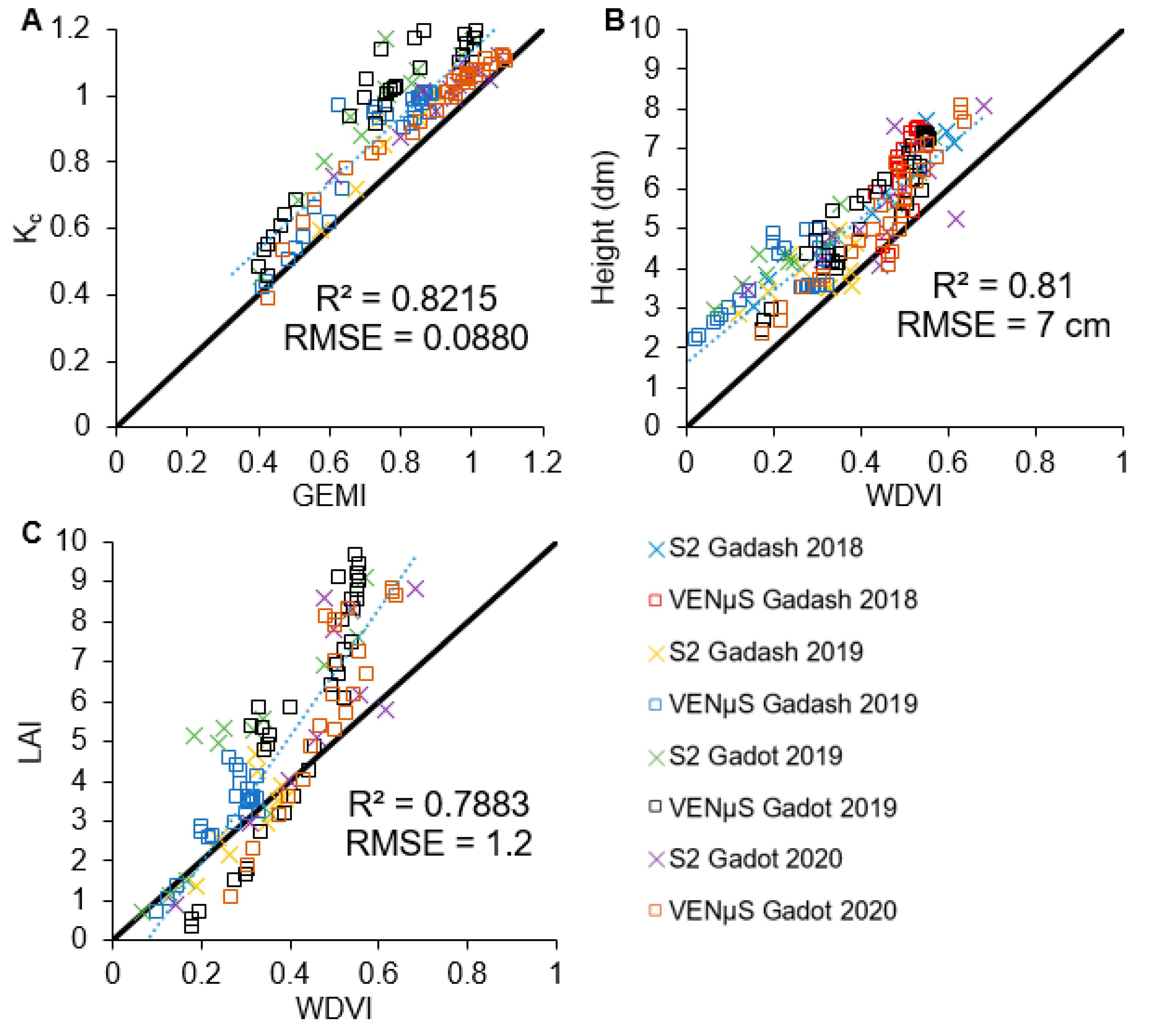
	All seasons	0.7544	1.2	0.7033	8	0.8215	0.0880
DVI	Sentinel-2 Gadash 2018				9
	VENµS Gadash 2018				8
	Sentinel-2 Gadash 2019		1.0		9		0.0568
	VENµS Gadash 2019		0.9		9		0.0795
	Sentinel-2 Gadot 2019		1.5		4		0.1155
	VENµS Gadot 2019		1.3		6		0.1161
	Sentinel-2 Gadot 2020		1.4		9		0.0864
	VENµS Gadot 2020		1.0		6		0.0963
	All seasons	0.776	1.2	0.7681	7	0.7756	0.0984
WDVI	Sentinel-2 Gadash 2018				8
	VENµS Gadash 2018				8
	Sentinel-2 Gadash 2019		0.7		7		0.0718
	VENµS Gadash 2019		1.2		10		0.0887
	Sentinel-2 Gadot 2019		2.1		9		0.1622
	VENµS Gadot 2019		1.2		5		0.1087
	Sentinel-2 Gadot 2020		0.9		6		0.0674
	VENµS Gadot 2020		1.1		6		0.1039
	All seasons	0.7418	1.3	0.7627	7	0.7431	0.1052
SAVI	Sentinel-2 Gadash 2018				9
	VENµS Gadash 2018				8
	Sentinel-2 Gadash 2019		1.2		10		0.0627
	VENµS Gadash 2019		1.0		9		0.0678
	Sentinel-2 Gadot 2019		1.5		5		0.1019
	VENµS Gadot 2019		1.4		7		0.1089
	Sentinel-2 Gadot 2020		1.0		8		0.0718
	VENµS Gadot 2020		1.1		7		0.0886
	All seasons	0.7637	1.2	0.7437	8	0.8138	0.0896
MSAVI	Sentinel-2 Gadash 2018				9
	VENµS Gadash 2018				8
	Sentinel-2 Gadash 2019		1.1		9		0.0590
	VENµS Gadash 2019		0.9		9		0.0737
	Sentinel-2 Gadot 2019		1.5		5		0.1087
	VENµS Gadot 2019		1.4		6		0.1136
	Sentinel-2 Gadot 2020		1.0		7		0.0737
	VENµS Gadot 2020		1.1		6		0.0948
	All seasons	0.7739	1.2	0.7612	8	0.7932	0.0944

Table 7. Performance statistics of newly developed S2/V_T-based LAI, Height, K_c models for the best performing VIs. Performance statistics of additional VIs can be found in Appendix D.

Vegetation Index	Dataset	LAI		Height		K_c
Vegetation Index	Dataset	R²	RMSE	R²	RMSE (cm)	R²	RMSE
GEMI	Sentinel-2 Gadash 2018				7
	VENµS Gadash 2018				9
	Sentinel-2 Gadash 2019		1.6		13		0.0798
	VENµS Gadash 2019		0.9		9		0.0714
	Sentinel-2 Gadot 2019		1.0		6		0.0944
	VENµS Gadot 2019		1.5		7		0.1183
	Sentinel-2 Gadot 2020		1.5		10		0.1120
	VENµS Gadot 2020		1.0		7		0.0713
	All seasons	0.7502	1.3	0.7101	8	0.7956	0.0942
DVI	Sentinel-2 Gadash 2018				7
	VENµS Gadash 2018				9
	Sentinel-2 Gadash 2019		1.3		10		0.0609
	VENµS Gadash 2019		0.8		8		0.0868
	Sentinel-2 Gadot 2019		1.3		4		0.0996
	VENµS Gadot 2019		1.4		7		0.1266
	Sentinel-2 Gadot 2020		1.3		8		0.1225
	VENµS Gadot 2020		1.0		6		0.0832
	All seasons	0.7731	1.2	0.7725	7	0.755	0.1028
WDVI	Sentinel-2 Gadash 2018				5
	VENµS Gadash 2018				8
	Sentinel-2 Gadash 2019		0.9		8		0.0531
	VENµS Gadash 2019		0.6		7		0.1038
	Sentinel-2 Gadot 2019		1.6		6		0.1286
	VENµS Gadot 2019		1.3		5		0.1167
	Sentinel-2 Gadot 2020		0.9		4		0.0901
	VENµS Gadot 2020		1.2		8		0.1161
	All seasons	0.7883	1.2	0.81	7	0.7214	0.1096
SAVI	Sentinel-2 Gadash 2018				7
	VENµS Gadash 2018				10
	Sentinel-2 Gadash 2019		1.7		12		0.0843
	VENµS Gadash 2019		0.8		8		0.0791
	Sentinel-2 Gadot 2019		1.2		4		0.0774
	VENµS Gadot 2019		1.6		8		0.1255
	Sentinel-2 Gadot 2020		1.4		9		0.1195
	VENµS Gadot 2020		1.0		6		0.0742
	All seasons	0.7383	1.2831	0.7317	8	0.7765	0.0982
MSAVI	Sentinel-2 Gadash 2018				6
	VENµS Gadash 2018				9
	Sentinel-2 Gadash 2019		1.6		12		0.0755
	VENµS Gadash 2019		0.8		8		0.0846
	Sentinel-2 Gadot 2019		1.3		4		0.0865
	VENµS Gadot 2019		1.6		7		0.1290
	Sentinel-2 Gadot 2020		1.4		9		0.1238
	VENµS Gadot 2020		1.0		6		0.0787
	All seasons	0.7484	1.3	0.7456	8	0.7585	0.1020

Table 8. Difference in performance statistics between newly developed S2/V_T and S2/V_NT-based LAI, Height, K_c models for the best performing VIs. Positive R² and negative RMSE indicate the superior performance of the S2/V_T model compared to the equal parameter of the S2/V_NT model. Significant differences are marked with (*). Performance statistics of the difference of additional VIs can be found in Appendix E.

Vegetation Index	Dataset	LAI		Height		K_c
Vegetation Index	Dataset	R²	RMSE	R²	RMSE (cm)	R²	RMSE
GEMI	Sentinel-2 Gadash 2018				−2
	VENµS Gadash 2018				1
	Sentinel-2 Gadash 2019		0.4		2		0.0159
	VENµS Gadash 2019		−0.2		−2		−0.0018
	Sentinel-2 Gadot 2019		−0.3		0		−0.0151
	VENµS Gadot 2019		0.1		1		0.0152
	Sentinel-2 Gadot 2020		0.2		1		0.0386
	VENµS Gadot 2020		−0.1		0		−0.0088
	All seasons	−0.0042	0.0	0.0068	0	−0.0259 *	0.0062
DVI	Sentinel-2 Gadash 2018				−2
	VENµS Gadash 2018				1
	Sentinel-2 Gadash 2019		0.3		2		0.0041
	VENµS Gadash 2019		−0.1		−1		0.0073
	Sentinel-2 Gadot 2019		−0.2		0		−0.0158
	VENµS Gadot 2019		0.1		1		0.0105
	Sentinel-2 Gadot 2020		−0.2		−1		0.0360
	VENµS Gadot 2020		0.0		0		−0.0131
	All seasons	−0.0029	0.0	0.0044	0	−0.0206	0.0044
WDVI	Sentinel-2 Gadash 2018				−3
	VENµS Gadash 2018				0
	Sentinel-2 Gadash 2019		0.2		2		−0.0187
	VENµS Gadash 2019		−0.6		−3		0.0151
	Sentinel-2 Gadot 2019		−0.5		−3		−0.0336
	VENµS Gadot 2019		0.1		0		0.0080
	Sentinel-2 Gadot 2020		0.0		−2		0.0227
	VENµS Gadot 2020		0.1		1		0.0122
	All seasons	0.0465	−0.1	0.0473*	−1	−0.0217	0.0044
SAVI	Sentinel-2 Gadash 2018				−3
	VENµS Gadash 2018				1
	Sentinel-2 Gadash 2019		0.5		3		0.0216
	VENµS Gadash 2019		−0.2		−1		0.0113
	Sentinel-2 Gadot 2019		−0.3		0		−0.0244
	VENµS Gadot 2019		0.2		1		0.0166
	Sentinel-2 Gadot 2020		0.4		2		0.0477
	VENµS Gadot 2020		−0.1		−1		−0.0144
	All seasons	−0.0254	0.1	−0.012	0	−0.0373 *	0.0086
MSAVI	Sentinel-2 Gadash 2018				−3
	VENµS Gadash 2018				1
	Sentinel-2 Gadash 2019		0.5		3		0.0165
	VENµS Gadash 2019		−0.2		−1		0.0109
	Sentinel-2 Gadot 2019		−0.3		0		−0.0222
	VENµS Gadot 2019		0.2		1		0.0154
	Sentinel-2 Gadot 2020		0.4		2		0.0501
	VENµS Gadot 2020		−0.1		−1		−0.0160
	All seasons	−0.0255	0.1	−0.0156	0	−0.0347 *	0.0076

Table 9. K_c prediction models based on field measurements of processing tomatoes height and LAI.

	K_c Prediction by Height	K_c Prediction by LAI
Measurements	24	21
R²	0.7467	0.6629
RMSE	0.0948	0.1024

Publisher’s Note: MDPI stays neutral with regard to jurisdictional claims in published maps and institutional affiliations.

© 2021 by the authors. Licensee MDPI, Basel, Switzerland. This article is an open access article distributed under the terms and conditions of the Creative Commons Attribution (CC BY) license (http://creativecommons.org/licenses/by/4.0/).

Share and Cite

MDPI and ACS Style

Kaplan, G.; Fine, L.; Lukyanov, V.; Manivasagam, V.S.; Malachy, N.; Tanny, J.; Rozenstein, O. Estimating Processing Tomato Water Consumption, Leaf Area Index, and Height Using Sentinel-2 and VENµS Imagery. Remote Sens. 2021, 13, 1046. https://doi.org/10.3390/rs13061046

AMA Style

Kaplan G, Fine L, Lukyanov V, Manivasagam VS, Malachy N, Tanny J, Rozenstein O. Estimating Processing Tomato Water Consumption, Leaf Area Index, and Height Using Sentinel-2 and VENµS Imagery. Remote Sensing. 2021; 13(6):1046. https://doi.org/10.3390/rs13061046

Chicago/Turabian Style

Kaplan, Gregoriy, Lior Fine, Victor Lukyanov, V. S. Manivasagam, Nitzan Malachy, Josef Tanny, and Offer Rozenstein. 2021. "Estimating Processing Tomato Water Consumption, Leaf Area Index, and Height Using Sentinel-2 and VENµS Imagery" Remote Sensing 13, no. 6: 1046. https://doi.org/10.3390/rs13061046

Note that from the first issue of 2016, this journal uses article numbers instead of page numbers. See further details here.

Article Menu

Estimating Processing Tomato Water Consumption, Leaf Area Index, and Height Using Sentinel-2 and VENµS Imagery

Abstract

1. Introduction

2. Materials and Methods

2.1. Test Sites and Field Measurements

2.2. Agro-Meteorological Measurements

2.3. Satellite Imagery

2.4. Vegetation Indices and Model Validation

3. Results

4. Discussion

5. Conclusions

Author Contributions

Funding

Data Availability Statement

Acknowledgments

Conflicts of Interest

Appendix A

Appendix B

Appendix C

Appendix D

Appendix E

References

Share and Cite

Article Metrics

Article Access Statistics

Further Information

Guidelines

MDPI Initiatives

Follow MDPI