Abstract
The accurate estimation of nearshore bathymetry is necessary for multiple aspects of coastal research and practices. The traditional shipborne single-beam/multi-beam echo sounders and Airborne Lidar bathymetry (ALB) have a high cost, are inefficient, and have sparse coverage. The Satellite-derived bathymetry (SDB) method has been proven to be a promising tool in obtaining bathymetric data in shallow water. However, current empirical SDB methods for multispectral imagery data usually rely on in situ depths as control points, severely limiting their spatial application. This study proposed a satellite-derived bathymetry method without requiring a priori in situ data by merging active and passive remote sensing (SDB-AP). It realizes rapid bathymetric mapping with only satellite remotely sensed data, which greatly extends the spatial coverage and temporal scale. First, seafloor photons were detected from the ICESat-2 raw photons based on an improved adaptive Density-Based Spatial Clustering of Applications with Noise (DBSCAN) algorithm, which could calculate the optimal detection parameters for seafloor photons by adaptive iteration. Then, the bathymetry of the detected seafloor photons was corrected because of the refraction that occurs at the air–water interface. Afterward, the outlier photons were removed by an outlier-removal algorithm to improve the retrieval accuracy. Subsequently, the high spatial resolution (0.7 m) ICESat-2 derived bathymetry data were gridded to match the Sentinel-2 data with a lower spatial resolution (10 m). All of the ICESate-2 gridded data were randomly separated into two parts: 80% were employed to train the empirical bathymetric model, and the remaining 20% were used to quantify the inversion accuracy. Finally, after merging the ICESat-2 data and Sentinel-2 multispectral images, the bathymetric maps over St. Thomas of the United States Virgin Islands, Acklins Island in the Bahamas, and Huaguang Reef in the South China Sea were produced. The ICESat-2-derived results were compared against in situ data over the St. Thomas area. The results showed that the estimated bathymetry reached excellent inversion accuracy and the corresponding RMSE was 0.68 m. In addition, the RMSEs between the SDB-AP estimated depths and the ICESat-2 bathymetry results of St. Thomas, Acklins Island, and Huaguang Reef were 0.96 m, 0.91 m, and 0.94 m, respectively. Overall, the above results indicate that the SDB-AP method is effective and feasible for different shallow water regions. It has great potential for large-scale and long-term nearshore bathymetry in the future.
1. Introduction
Acquiring detailed bathymetric and topographic information in coastal areas is one of the challenges for both hydrology-related studies and water resource management. High-resolution underwater topography data are a basic reference for a wide range of coastal applications, such as hydrological investigation, nearshore protection, and marine mineral resources exploitation. Conventionally, shipborne single-beam/multi-beam echo sounders and Airborne Lidar bathymetry (ALB) are mainstream technologies used to collect shallow coastal water data and deliver near-constantly underwater topographies [1,2,3,4,5,6]. However, the disadvantages of these two methods are obvious. They have a high cost, are inefficient, and have sparse coverage [7,8,9,10,11].
Satellite-derived bathymetry (SDB) is a crucial alternative measurement used to map coastal water bodies of the world. Traditional SDB methods in shallow water can be divided into two methodological categories: empirical and physics-based [12]. SDB empirical methods tend to model the radiative transformation in water to process optical images, which are mainly discussed in this paper. SDB empirical methods were first associated with multispectral imagery technology in 1978 [13]. Then, spaceborne multispectral sensors (e.g., Sentinel-2/Multispectral Instrument (MSI), LandSat-1/Multispectral Scanner (MSS), and LandSat-8/Operational Land Imager (OLI)), which are typical passive remote sensing techniques, have been widely used for bathymetry [14,15,16,17,18,19,20]. They can realize bathymetry in optimal conditions (<30 m depth) [21]. However, empirical SDB methods using multispectral imagery technology generally rely on in situ depths as control points, or SDB is independent of control data through complicated physics-based approaches to derive bathymetric data [17,22]. Therefore, it is not feasible to obtain ground, shipborne, or airborne-based measurement data in remote locations of the world. With the development of photon-counting sensors, spaceborne photon-counting lidars show many advantages of bathymetry mapping. In conjunction with passive multispectral measurements, space-based lidar can provide complementary, vertical profiling for superior depth penetration and vertical accuracy. The new Ice, Cloud, and Land Elevation Satellite-2 (ICESat-2) has great potential to fill in this gap since it carries the Advanced Topographic Laser Altimeter System (ATLAS)—the first Earth-orbiting laser that is capable of penetrating water at a high resolution in the along-track direction [23].
The National Aeronautics and Space Administration (NASA) launched ICESat-2 on 15 September 2018. ATLAS operates at 532 nm and emits three pairs of beams spaced 3.3 km apart with a 90 m distance within pairs [24]. Each pair of beams consists of a strong beam, and a weak beam based on a 4:1 transmit energy ratio, and each beam samples with an interval of ~70 cm along the orbit and only has a ~14 m diameter footprint [25,26]. ICESat-2 has the advantage of global coverage, including areas where high-resolution or up-to-date bathymetry is not available [27]. In addition, ATLAS can collect along-track bathymetric points up to 40 m in depth in very clear water [23]. Therefore, the bathymetric photon points from ICESat-2 can provide complementary datasets which work as in situ depth control points on SDB empirical models.
ICESat-2 ATLAS penetrated the water as an active lidar and has been applied to the expression of the Earth’s surface topography. ATLAS determined the surface slope on ice sheets and tracked the evolution of a sea ice pack and freeboard in winter [28,29]. ICESat-2 makes considerable improvements, particularly the dense along-track sampling of the surface, which helps obtain highly detailed bathymetry information in shallow water [30]. A method was proposed to estimate the temporal change in water levels and volumes with Multiple Altimeter Beam Experimental Lidar (MABEL) data [31]. MABEL served as a technology demonstrator of ICESat-2 ATLAS. Based on the actual ICESat-2 data, an adaptive variable ellipse filtering bathymetric method was proposed to precisely identify and separate the photons in the above-water, water surface, and water-column regions [32]. Some studies have combined ICESat-2 ATLAS with passive remote sensing techniques into bathymetry retrieval in recent years [33,34]. The ATLAS dataset could work as a complementary dataset, which offers flexibility on bathymetry. According to the signal characteristics of ATLAS, the clustering density method has been proven to be effective for photon signal processing [35,36]. These studies have proved that this fusion method is now feasible between satellite-based multispectral images and Lidar data.
However, there are still some barriers to be solved. Due to the optical characteristics of ATLAS, the raw photon data include a great deal of solar background noise photons, which require the development of specialized onboard receiver algorithms that can distinguish signals containing surface returns from those consisting of pure noise [26]. Current methods for valid photons detection partly rely on preview empirical parameters [35] and even classify points manually [36], which cannot be used for batch data processing. In addition, these methods could not overcome the limitations of large scales and different underwater terrains. To address these problems, the adaptive methods for automated processing of the ATLAS photon data are needed and need to be improved to achieve spatial coverage and depth measurements.
In this study, a satellite-derived bathymetry method merging active and passive remote sensing (SDB-AP) in shallow waters and coastal areas is proposed. It merges both active (i.e., ICESat-2) and passive (i.e., Sentinel-2 satellite) satellite datasets and applies an adaptive Density-Based Spatial Clustering of Applications with Noise (DBSCAN) algorithm, which greatly extended spatial coverage and bathymetric inversion accuracy. First, we detected seafloor return photons from the ICESat-2 raw photons based on an improved adaptive DBSCAN algorithm. Then, we corrected the detected seafloor photons due to the refraction at the air–water interface. After, we applied a suitable outlier-removal algorithm to remove outlier photons to improve the retrieval accuracy. We divided all of the ICESate-2 seafloor signal photons randomly into two parts: 80% of gridded data as control points were used to train the empirical bathymetric model, and the remaining 20% as well as the in situ data collected by the NOAA’s National Centers for Environmental Information (NCEI) were used to quantify our inversion scheme’s accuracy. We produced several bathymetric maps over St. Thomas, Acklins Island, and Huaguang Reef using the empirical bathymetric model trained by merging the ICESat-2 data and the Sentinel-2 multispectral images. Finally, we evaluated and analyzed the performance of our method.
2. Study Areas and Data Sources
2.1. Study Areas
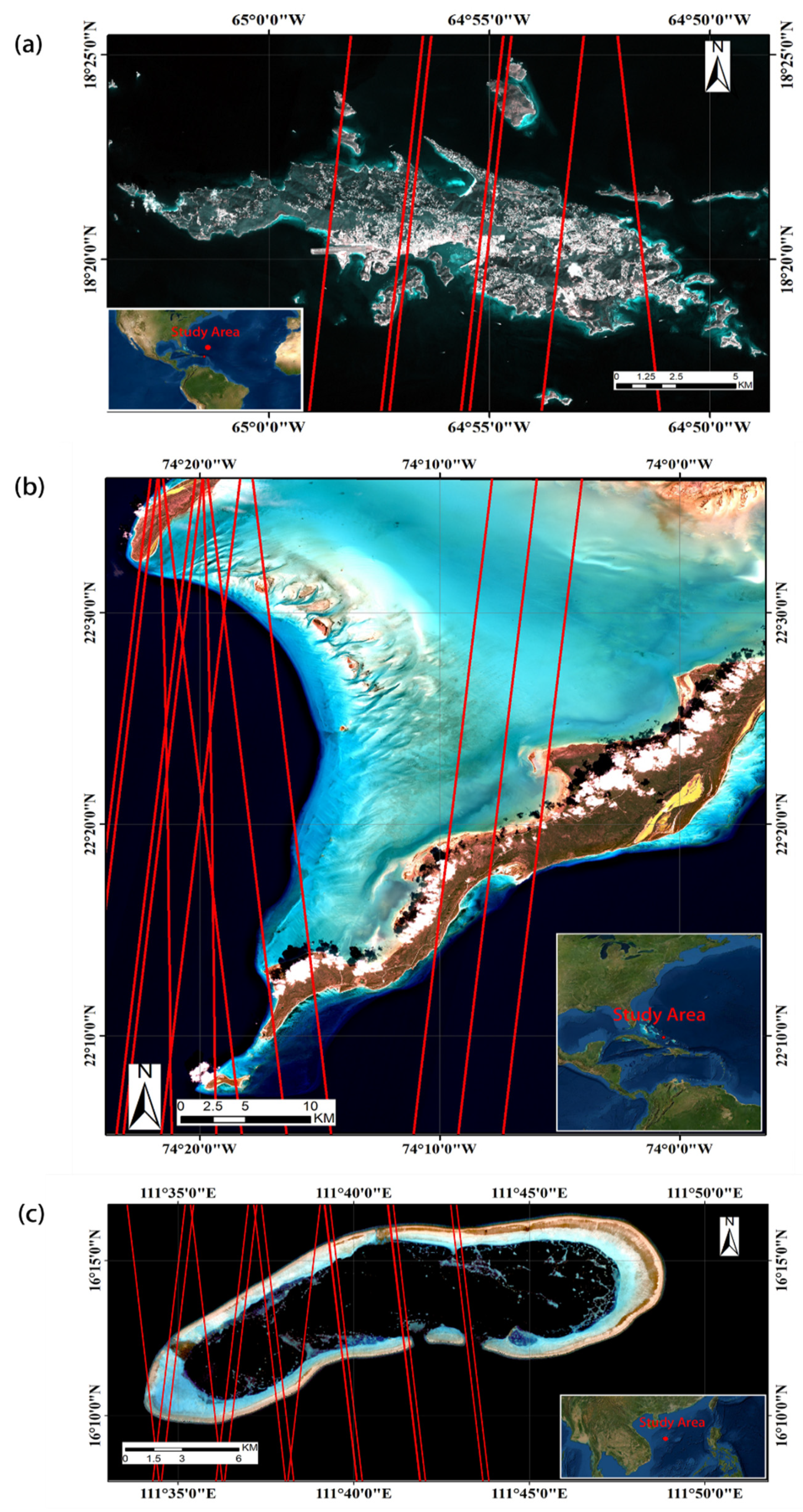
Three study regions with different topographic distributions were chosen to obtain the satellite bathymetric map. The first region, named Saint Thomas (St. Thomas), as Figure 1a shows, is the second-largest island of the US Virgin Islands in the eastern Caribbean Sea. The district has a land area of about 83 km2 [37]. The geographical location of this area is between 18.26°~18.43°N and 64.80°~65.0°W. The Continuously Updated Digital Elevation Model (CUDEM) obtained in December 2014 for the US coast developed by NCEI, was used as in situ data to verify the performance of our bathymetric method in St. Thomas [38]. The second study region, as Figure 1b shows, was the surrounding waters around Acklins Island and Long Cay in Southeastern Bahamas. The geographical location of this area is between 22.10°~22.60°N and 73.90°~74.40°W. There is a lagoon between Acklins Island and Long Cay. The bottom is mainly reef, sand, and stone. The third study region, as Figure 1c shows, was the Huaguang Reef. Huaguang Reef is one of the main reefs of Xisha Islands in the northwestern South China Sea, about 330 km away from Hainan Island. The geographical location of this area is between 16.13°~16.28°N and 111.52°~111.86°E. There are several coral reefs in the region. In all three sites, the in situ bathymetric data are not easy to access to evaluate the empirical SDB model; therefore, we applied ICESat-2 bathymetric photons to evaluate bathymetric maps based on SDB-AP. A total of 80% of the ICESat-2 bathymetric points were used to train the empirical model, and the remaining 20% were used to verify the SDB-AP bathymetric result. In addition, we discuss Chen’s method [32] along with our method; thus, we chose two sites (Shanhu Island and Nan Island) and the corresponding ICESat-2 tracks (see Table 1). According to Chen’s definition, the photon density of ICESat-2 track data on 2 February 2019, 24 May 2019, and 19 August 2019 are low, medium, and high, respectively. Three types of ICESat-2 data with different density distributions of photons can help to validate the accuracy of these DBSCAN algorithms.
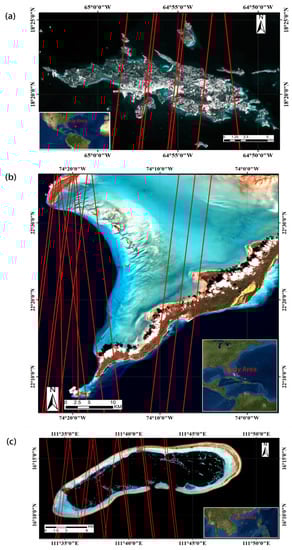
Figure 1.
Overviews of three study areas: (a) Saint Thomas, US Virgin Islands—the background satellite image belongs to Sentinel-2 acquired on 15 January 2019. All red lines correspond to the laser trajectories of ICESat-2 on 22 November 2018, 10 February 2019, and 13 December 2020, respectively. A total of 80% of the ICESat-2 bathymetric points were randomly used to train the empirical model, and the remaining 20% as well as in situ data were used to verify the SDB-AP bathymetric result. (b) Acklins Island—the satellite image in the background belongs to Sentinel-2 acquired on 27 January 2020. All red lines correspond to the laser trajectories of ICESat-2 on 12 November 2018, 11 February 2019, 12 March 2019, 3 June 2019, and 2 September 2019. 80% of the ICESat-2 bathymetric points were used to train the empirical model, while the remaining 20% were used to verify the SDB-AP bathymetric result. (c) Huaguang Reef—the satellite image in the background belongs to Sentinel-2 acquired on 13 August 2019. All red lines correspond to the laser trajectories of the ICESat-2 on 22 October 2018, 22 February 2019, 21 April 2019, 19 April 2020, 19 July 2020, and 20 August 2020. 80% of the ICESat-2 bathymetric points were used to train the empirical model, while the remaining 20% were used to verify the SDB-AP bathymetric result.

Table 1.
Detailed information of the study areas and the ICESat-2 and Sentinel-2 datasets.
2.2. ICESat-2 Lidar Datasets
The first spaceborne photon-counting lidar ATLAS carried by ICESat-2 can provide supplementary, vertical profiling for superior depth penetration and vertical accuracy. ICESat-2 has been collecting data since 14 October 2018. Each captured photon has a unique delta-time, latitude, longitude, and elevation based on the World Geodetic System 1984 (WGS84) ellipsoid datum. ICESat-2 has a set of data products, including the Global Geolocated Photon Level 2A data product ATL03. ATL03 is a large dataset comprising latitude, longitude, and ellipsoidal height for every detected photon event. ICESat-2 photon data we used in this study can be freely downloaded from the National Snow & Ice Data Center website [39]. ATL03 data includes the height above the WGS84 datum (ITRF2014 reference frame) and in the universal transverse Mercator (UTM) [40].
In ATL03 datasets, the “signal_conf_ph” parameter in the /gtx/heights group for each beam refers to the confidence parameter provided to classify photons that are likely surface-reflected signal photons and those that are likely background photons [41]. The “signal_conf_ph” array has five values for each photon, corresponding to five surface types (land, ocean, sea ice, land ice, and inland water). The specific values range from 4 to −2 [42]. The photon classification algorithm is histogram-based which may classify a background photon incorrectly as a signal photon because of the false threshold. The higher the confidence (from 0 to 4) means the higher possibility of the photons being a signal. It is noticeable that the high confidence (4) photons do not include all signal photons, especially seafloor signal photons. We also noticed that the confidence four photons were mostly the signal from the objectives of high reflectivity, such as sea surface and land. To improve the usage of this parameter, an adaptive DBSCAN algorithm was proposed to detect the signal photons without detection radius and a threshold priori, and the confidence of the four photons was used to help determine the positions of the sea surface in this algorithm.
2.3. Sentinel-2 Satellite Imagery
Sentinel-2 Level-1C (L1C) imagery products can be freely downloaded in SENTINEL-SAFE format from the US Geological Survey website (USUG) [43]. All of the downloaded L1C images are in the UTM/WGS84 projection, and they are orthophoto images after geometric correction [44]. To reduce random errors caused by the atmosphere, we tried to choose a total of three Sentinel-2 L1C images with less than 20% cloud coverage. Detailed information on all study areas and the ICESat-2 and Sentinel-2 datasets are shown in Table 1.
3. SDB-AP Method
3.1. Adaptive DBSCAN for ICESat-2 Signal Photon Detection
The DBSCAN algorithm has been proven to be a classic and efficient way to detect ground and seafloor photons from photon-counting lidar signal returns [19,28]. In the DBSCAN algorithm, when the density of adjacent points in radius exceeds the threshold (), the points in the cluster are classified as signals; thus and are the key parameters [45]. Standard DBSCAN algorithms rely on preview empirical parameters of and [35]. The determination of adaptive threshold and could be helpful for automated batch processing and could improve the detection algorithm accuracy. An improved adaptive DBSCAN algorithm for ICESat-2 signal photon detection was proposed as follows, and detailed processing steps are provided in Appendix A.
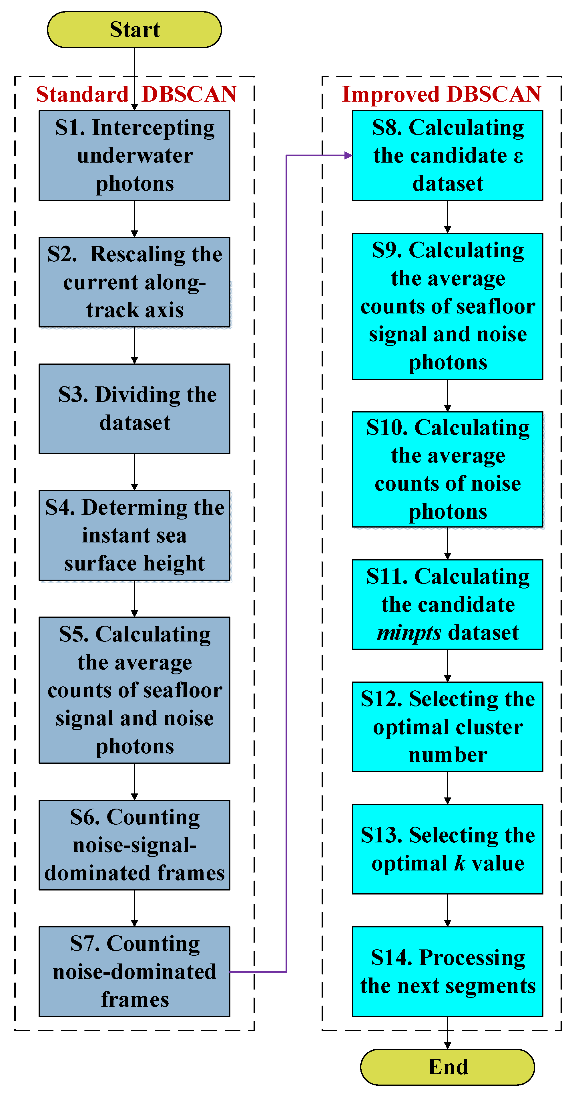
First, we intercepted the underwater photons and rescaled the current along the track axis to avoid calculation errors from rounding . Then, we divided the dataset into several segments. For each segment, we determined the instant sea surface height (SSH) and calculated the average counts of seafloor signal and noise photons. After that, we counted the noise–signal-dominated frames and noise-dominated frames. We calculated the candidate dataset. According to the candidate dataset, the average counts of seafloor signal and noise photons and the average counts of noise photons could be computed, and we obtained the candidate dataset. Finally, we selected the optimal and by iteration. Our adaptive DBSCAB codes were completed on the Python 3.9 platform. The flowchart for the adaptive DBSCAN algorithm is shown in Figure 2.
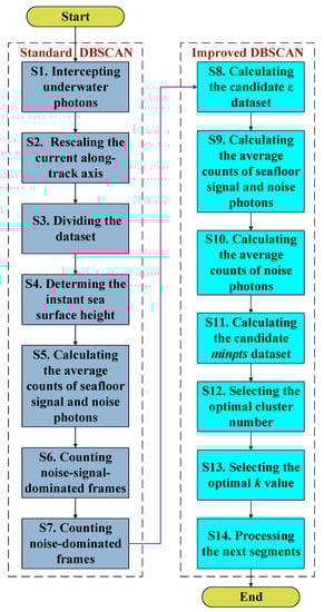
Figure 2.
The flowchart for the adaptive DBSCAN algorithm.
3.2. Bathymetric Correction for Detected Seafloor Photons
ICESat-2 products do not consider the refraction and the corresponding change in light speed at the air–water interface. This will produce horizontal and vertical errors in the geolocation recorded in ATL03, resulting in the position being deeper than the real measurement value and farther from the lowest point; thus, ICESat-2 ATLAS needs appropriate refraction corrections.
The refraction correction method proposed by Parrish was applied [23]. The final underwater return photon depth could be expressed as follows:
where is the uncorrected depth of the underwater photons detected by the adaptive DBSCAN method, is the slant range to the uncorrected bottom return photon location, is the corrected slant range, is the angle of incidence, and is the angle of refraction. In Equation (1), could be expressed as follows:
3.3. Outlier Removal for Corrected Seafloor Photons
The purpose of outlier detection is to filter abnormal data in each dataset. In other words, the main goal of outlier detection is to find outliers or noises markedly different from or inconsistent with the normal instances. The corrected seafloor photon points still contained a few noise photons [46]; therefore, we proposed an outlier-removal method for seafloor photons as follows:
- I.
- Wavelet filteringA hard threshold was optimally set according to the noise level estimation of each layer of the wavelet decomposition.
- II.
- K-medoids classificationThe data were divided into three categories by the K-medoids algorithm [47]. In the K-medoids algorithm, such a point would be selected from the current cluster—the minimum sum of the distances from it to all other points (in the current cluster)—as the center point, which allows the cluster size not to vary greatly.
- III.
- Outlier removal along the geographic axisThe data were sorted along the ICESat-2 along-track first. For each category, the outliers were detected and eliminated using scaled mean absolute difference MAD, and these outliers were eliminated with a window size of 50. The outliers were defined as the elements that differ from the median by more than three scaled from the median in the window. could be expressed as follows:where .
- IV.
- Outlier removal along the depth axisThe remaining data were then processed. The outliers were defined as the elements more than three scaled in data with the window size of 100, and the recognized outliers were removed.
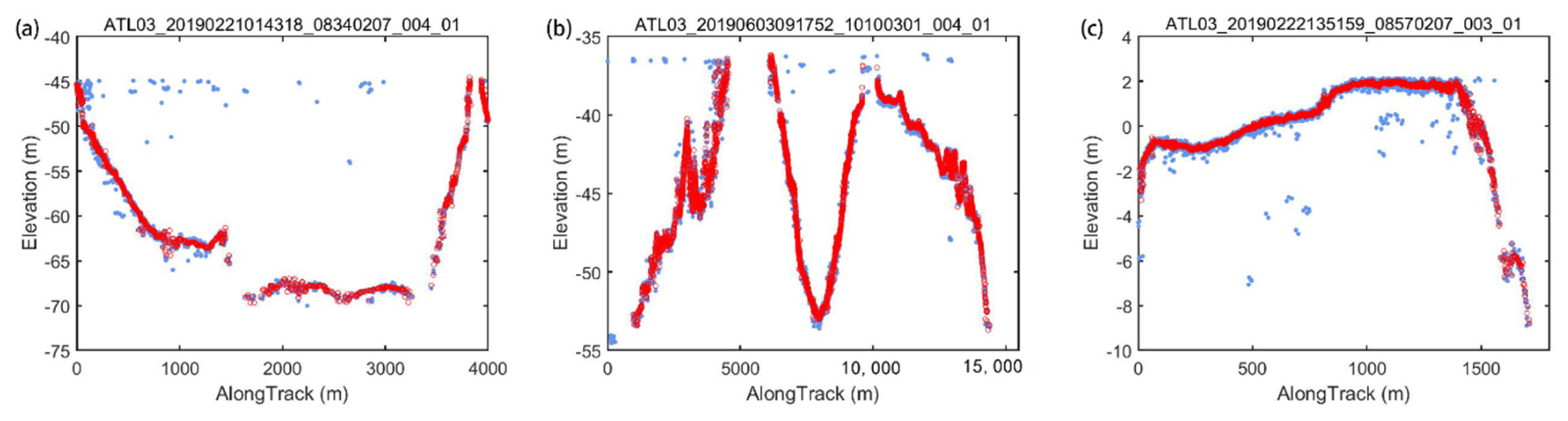
Here are three examples that present the outlier-removal results from the ICESat-2-derived signal photons in Figure 3a–c. The light blue points correspond to the noise photons, and the red points are seafloor photons after noise-outlier removal. It can be noted that our algorithm cleared out most outlier points and reserved seafloor signal photons efficiently.
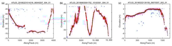
Figure 3.
Outlier-removal result based on our method with the noise photons (light blue) and the outlier-removal signal photons (red): (a) St. Thomas site, (b) Acklins Island site, and (c) Huaguang Reef site.
3.4. Matching ICESat-2 Data to Sentinel-2 Images with Different Spatial Resolution
The spatial resolution of ICESat-2 and in situ depth data are higher than that of Sentinel-2 image data, which means the depth value of each pixel of the Sentinel-2 bathymetric map may correspond to a great deal of high spatial resolution control points or in situ points in the process of depth inversion. To solve this problem, it is necessary to reduce the high-resolution data to the Sentinel-2 spatial resolution (10 m).
The ICESat-2 data with high spatial resolution were matched with the Sentinel-2 pixel in the WGS-84 coordinate reference system, according to the same latitude and longitude range, and the average value was obtained from the data corresponding to each pixel value of Sentinel-2 data. During the averaging process, the Pauta criterion of the mean plus or minus three standard deviations (SD) was utilized based on the characteristics of a normal distribution for which 99.87% of the data appear within this range [48]. Therefore, each mean depth corresponded to a Sentinel pixel, and the down-sampled dataset was used to build the empirical model.
3.5. SDB Retrieval by Merging the Sentinel-2 Data with ICESat-2 Data
3.5.1. Atmosphere Correction
Before the application of the SDB empirical model, all the raw Sentinel-2 L1C products in study areas needed to be atmospherically corrected and conveyed to Level-2A (L2A) products containing bottom-of-atmosphere (BOA) corrected reflectance [49]. The Sentinel-2 Data Correction (Sen2Cor) version 2.9 was chosen for atmospheric correction [50]. Sen2Cor is a semi-empirical algorithm based on the Atmospheric and Topographic Correction (ATCOR) and can be applied over water surfaces. European Space Agency (ESA) provides an offline version of the Sen2Cor to produce L2A data. The first step is cloud detection and scene classification, followed by retrieving the Aerosol Optical Thickness (AOT) and the Water Vapor (WV). Finally, Top-Of-Atmosphere (TOA) is converted to Bottom-Of-Atmosphere (BOA) [51]. Considering the spatial resolution for each visible band (B2—497 nm, B3—560 nm, and B4—665 nm), a spatial resolution of 10 m was used in Sen2Cor processing. Thus far, the raw Sentinel-2 L1C image was converted to the processed L2A image.
3.5.2. Spatial Operation
The L2A images needed a spatial operation to simplify our analysis and focus on the region of interest (ROI). First, we resampled all bands to equal resolution. In the resampling, we selected band B2 as the reference band. Then, we could create subsets of ROI in each resampled L2A image.
3.5.3. Clouds, Whitecaps, and Land Pixels Mask
Masks were generated to remove clouds, whitecaps, and land pixels. The Near Infrared (NIR) band is used to mask clouds, whitecaps, and most land pixels; since the NIR does not penetrate the water, the water seems darker, which helps to distinguish the water from the things that look brighter. We used a user-set threshold value (0.05) of the NIR band and created the mask with this threshold; by applying this mask to each band, we created a masked image that only contains sea with original values and invalid value NaN for the ocean and the others, respectively. For the land pixels mask, we downloaded a course Space Shuttle Radar Topography Mission (SRTM) 5-min Digital Elevation Model [43], which can determine whether the pixel is on land. Then, we created a new image so that all ocean pixels would be preserved, and all land pixels would be set to NaN, and all Sentinel-2 images were projected to the same WGS-84 coordinate reference system before empirical bathymetric inversion.
3.5.4. Empirical SDB Retrieval
Finally, the ratio model was conducted to calculate seafloor depths using the depth control points from ICESat-2-derived bathymetry described in Section 3.3. The ratio model is expressed as follows:
where is the estimated depth, is a tunable constant to scale the ratio to depth, is a fixed constant for all areas (usually 1000), is the reflectance of water for bands or , and is the offset for a depth of 0 m (). and were calculated by regression using the depth control points from ICESat-2 derived bathymetry.
The flowchart of the SDB-AP method is shown in Figure 4. The whole SDB-AP codes and partly ICESat-2 bathymetry data are available online in Supplementary Materials.
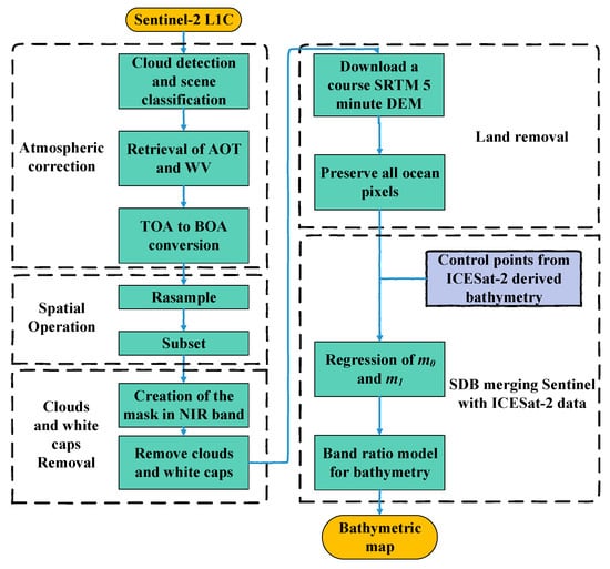
Figure 4.
The flowchart of the SDB-AP.
4. Results
4.1. Bathymetric Retrieval by ICESat-2 Data
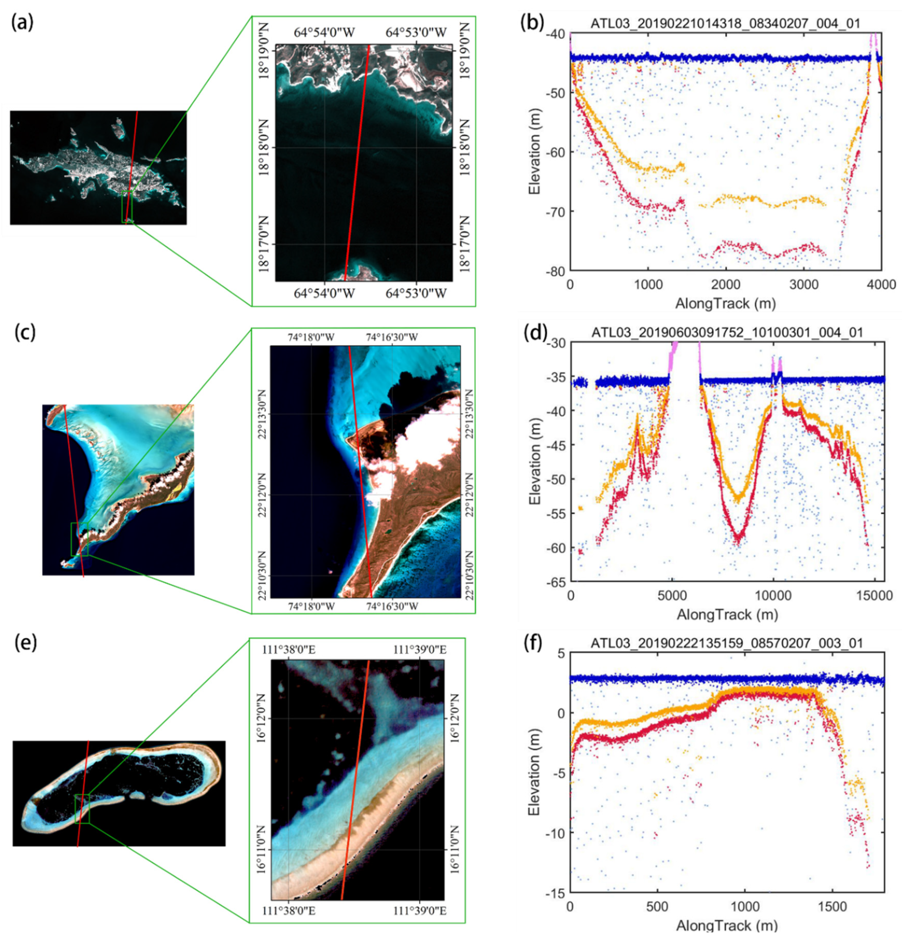
Based on our proposed algorithm in Section 3.1 and Section 3.2, the ICESat-2 signal photons were detected. Figure 5 provides ICESat-2 ground trajectory images, and corresponding detected elevation profiles over the St. Thomas site, Acklins Island site, and Huaguang reef site. Figure 5a,c,e demonstrates the enlarged satellite image and the sampled areas corresponding to the green box. Figure 5b,d,f illustrates the detected ICESat-2 underwater photons with and without refraction correction.
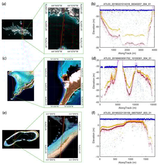
Figure 5.
Enlarged satellite images and profiles of geolocated photon returns over three study sites: (a,b) St. Thomas on 21 February 2019; (c,d) Acklins Island on 3 June 2019; (e,f) Huaguang Reef on 22 February 2019; bathymetric retrieval by ICESat-2 data over the St. Thomas site with the detected seafloor signal photons (red), the corrected seafloor photons from our detected result photons(orange), the detected sea surface (dark blue), and the noise photons (light blue).
Figure 5a shows that ICESat-2 flew over this area at the local time of 01:43:18 on 21 February 2019. from north to south. The satellite first flew over a shallow water region and then went over a deep underwater terrain and quickly back to a shallow area. In Figure 5b, significant seafloor signal photons were detected by ICESat-2 in accordance with underwater topography. For each laser shot, the refraction effect in the water column was corrected by the equations in Section 3.2. The maximum profile of the refraction-corrected bottom return photons was about ~70 m, while ICESat-2 detected seafloor signal photons nearly reached ~80 m. Therefore, without the refraction correction in vertical elevation, the same water level errors influence the bathymetry results. The maximum bathymetric depth over St. Thomas was larger than that over the other two sites. Figure 5c shows that ICESat-2 flew over this area at the local time of 09:17:25 on 13 June 2019, from south to north. The trajectory was over two land margins of Long Cay. In Figure 5d, it is noticeable that our DBSCAN results matched well with underwater topography, and even the seafloor details were scanned accurately. The maximum refraction-corrected return photons were up to the water depth of ~20 m. Figure 5e shows that ICESat-2 flew over this area at the local time of 13:51:59 on 22 February 2019, from north to south. The satellite passed by a part of a reef and then went to a deep-water area. In Figure 5f, our DBSCAN results were consistent with underwater topography, and the maximum refraction-corrected return photon depth was ~8 m. The maximum bathymetric depth over Huaguang Reef was the smallest.
4.2. Bathymetric Retrieval by the SDB-AP
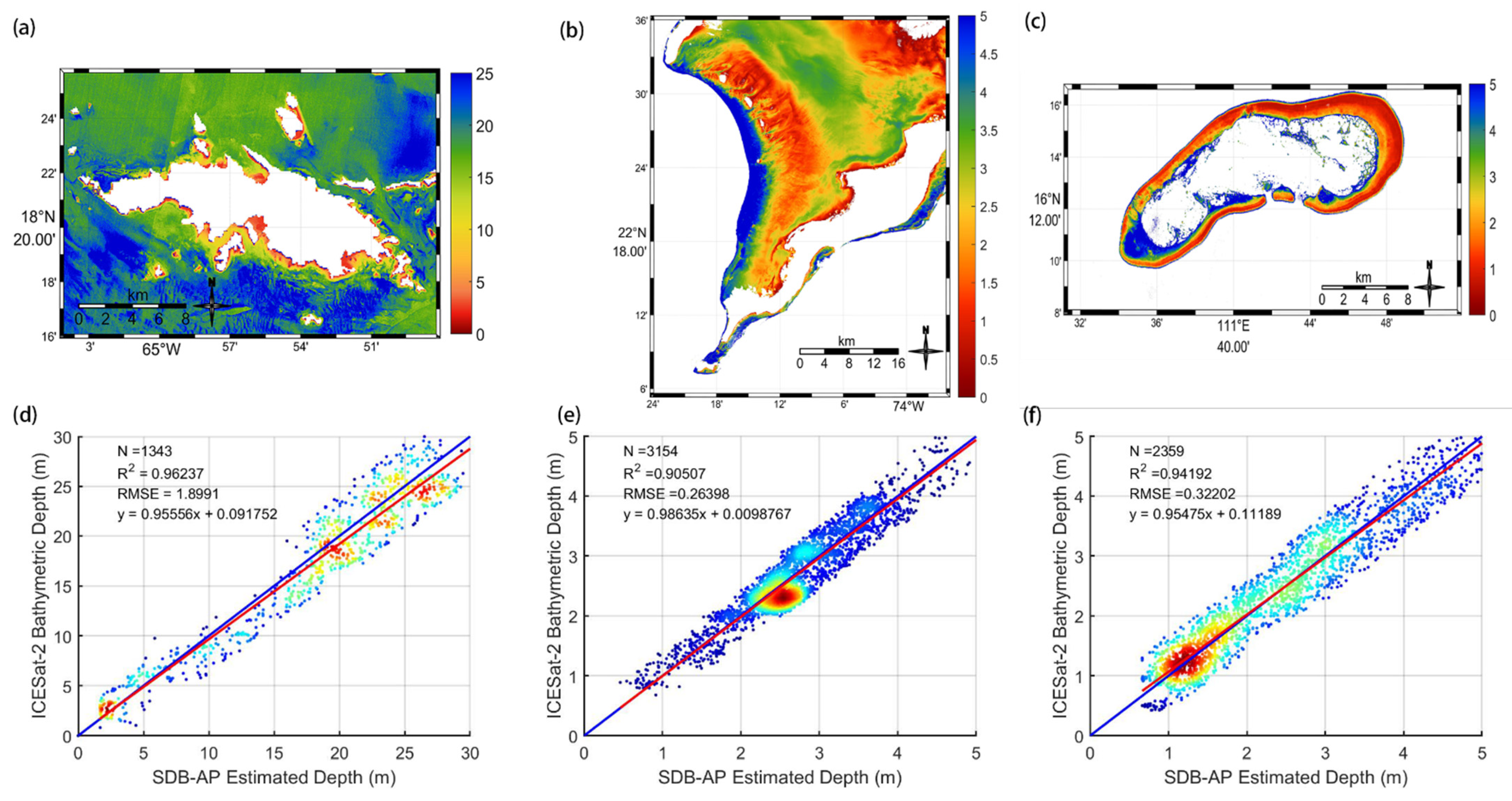
Figure 6a–c shows the bathymetric maps over the St. Thomas site, Acklins Island site, and Huaguang Reef site based on the SDB-AP. Over the St. Thomas site, the blank area is the land masked by the course SRTM 5-min DEM. The maximum and minimum bathymetric depths were 34.79 m and 2.29 m in Figure 6a, respectively. The water depth in the north was shallower than that in the south, and the coastal water depth was shallow. The average depth was 18.83 m in total. Over the Acklins Island site, we present a bay within the depth of 5 m, where the average bathymetric depth was 2.83 m. From west to east, the bathymetric depths presented a fluctuating state, and the margin of the area was towards the deep water in Figure 6b. The maximum bathymetric depth was 9.87 m. Over the Huaguang Reef site in Figure 6c, which is a submerged reef in the South China Ocean, the maximum, minimum, and average bathymetric depths were 13.88 m, 0.37 m, and 3.08 m, respectively.
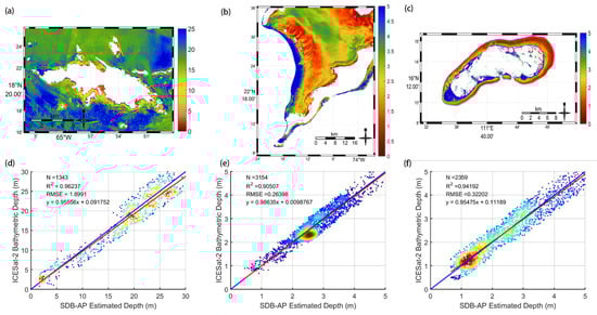
Figure 6.
SDB-AP derived-bathymetric maps and error scatter plots of SDB-AP estimated depths vs. ICESat-2 bathymetric depths: (a) derived bathymetric maps in the St. Thomas site, (b) derived bathymetric maps in the Acklins Island site, (c) derived bathymetric maps in the Huaguang Reef site, (d) error scatter plots in St. Thomas site, (e) error scatter plots in the Acklins Island site, and (f) error scatter plots in the Huaguang Reef site. The red line is the 1:1 line, while the blue line represents the regression line. is the number of the training gridded bathymetric points from ICESat-2, and the regression equation details are shown in the top-left corner.
4.3. Validation
For all study sites, 80% of the detected ICESat-2 derived bathymetric photon points were used as model-training points, and the remaining 20% were used to validate the method’s validation accuracy. The in situ data over the St. Thomas site were also employed to quantify the performance of SDB-AP. In the following error scatter plots, the red line is the 1:1 line, and the blue line represents the regression line. is the number of the training gridded bathymetric points from ICESat-2, and the regression equation, R2, and RMSE details are also shown in the figures.
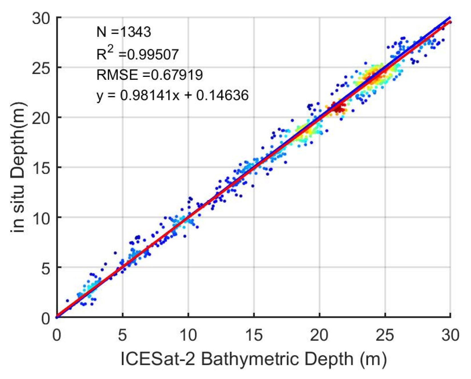
In Figure 7, the ICESat-2-derived bathymetric depths matched well with the in situ data over St. Thomas, with a good agreement of R2 = 0.9951 and a low standard Root Mean Squared Error (RMSE) at 0.68 m, which proves that our adaptive DBSCAN and outlier-removal algorithm are effective. For SDB-AP-estimated depths and the in situ data over St. Thomas, R2 was 0.93, and the RMSE was 1.91 m, as shown in Figure 8. Compared with the ICESat-2-derived bathymetric depths, the bathymetric accuracy of SDB-AP estimated depth decreases due to the error accumulation effects, including the ICESat-2 inversion error, the spatial matching error between ICESat-2 and Sentinel data, the Sentinel image process error, the empirical SDB model error, etc. Among them, the empirical SDB model error is the main error source; generally, the error for the empirical SDB model is about 2 m [15,17,18,20]. Figure 6d–f shows the performance of SDB-AP estimated depths when the ICESat-2-derived bathymetric points were used as testing data in the three study areas. The R2 in St. Thomas site reached the top (R2 = 0.96), followed by that in the Huaguang Reef site and Acklins Island site, 0.94 and 0.91, respectively. All RMSEs in the St. Thomas site, Acklins Island site, and Huaguang Reef site were less than 10% of the maximum depths, and the smallest RMSE was in the Acklins Island site with the value of 0.27 m.

Figure 7.
Error scatter plot: ICESat-2 bathymetric depths vs. in situ depths over St. Thomas. The red line is the 1:1 line, while the blue line represents the regression line. is the number of the training gridded bathymetric points from ICESat-2, and the regression equation details are shown in the top-left corner.
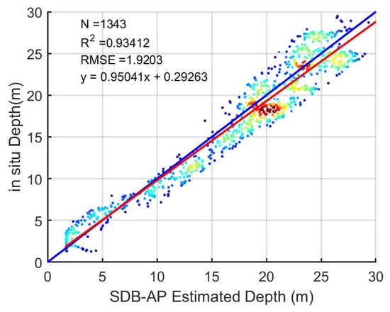
Figure 8.
Error scatter plot: SDB-AP estimated depths vs. in situ depths over St. Thomas. The red line is the 1:1 line, while the blue line represents the regression line. N is the number of training gridded bathymetric points from in situ data, and the regression equation details are shown in the top-left corner.
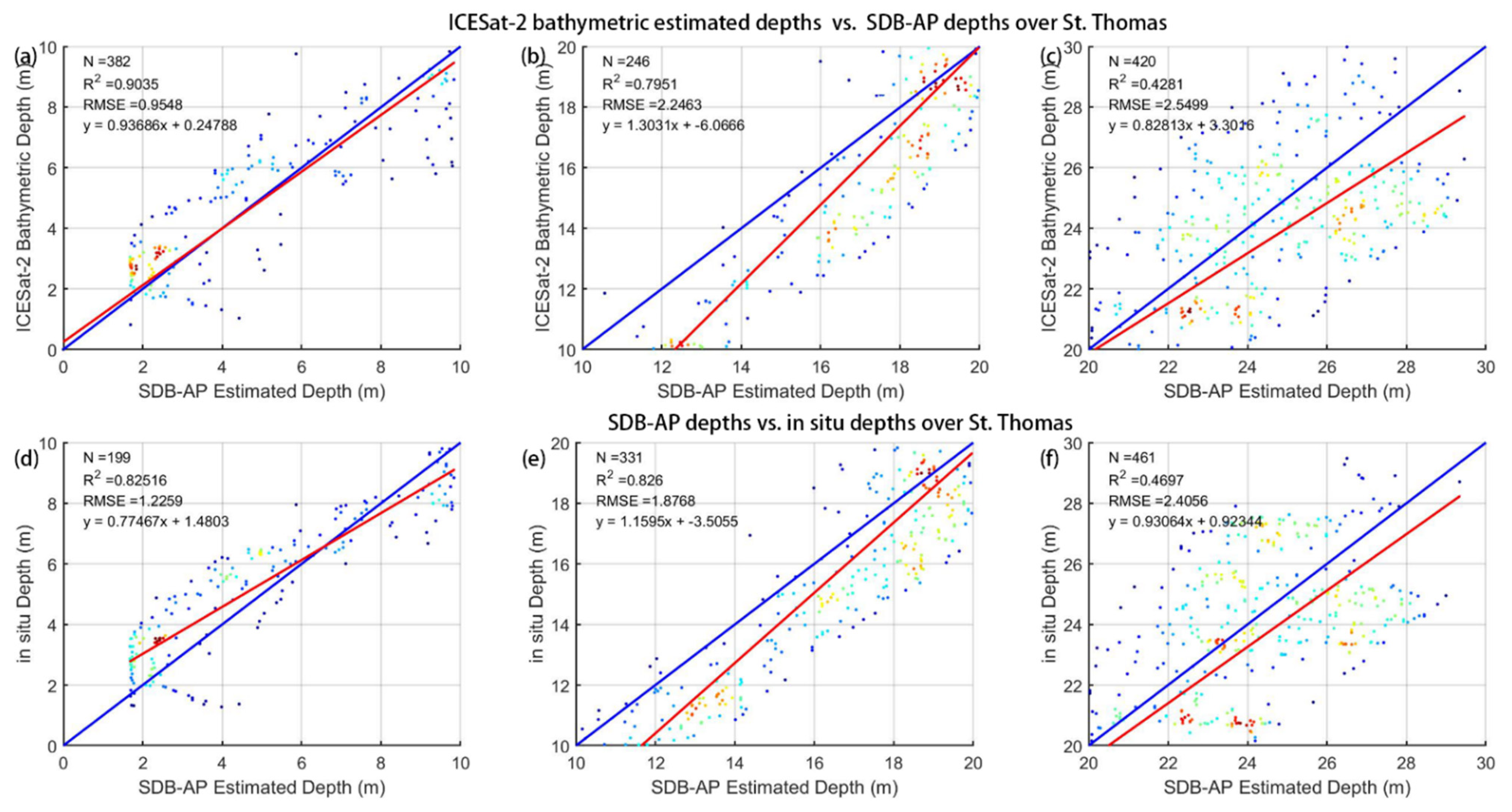
Figure 9a–c illustrates the error scatter plots in different depth ranges over St. Thomas. The horizontal axis and the vertical axis in Figure 9a–f are the SDB-AP estimated depths versus the ICESat-2 bathymetric estimated depth and the SDB-AP estimated depth versus the in situ depth, respectively. In Figure 9a–c, the trend of scattered points was visually linear at a depth of 0–10 m, started to diverge when the water depth was between 10 and 20 m, and finally dispersed over 20 m. The same trend could be noticed in Figure 9d–f. Table 2 and Table 3 present the error analysis in different depth ranges. Table 2 corresponds to the information for Figure 9a–c, and Table 3 corresponds to the information for Figure 9d–f. It appears that the , RMSEs and Mean Absolute Error (MAEs) rose with the increase in water depth, while the R2 fell, which revealed that there were large errors in deep water (>20 m) and that the SDB is more feasible for shallow water within a depth of 10 m.
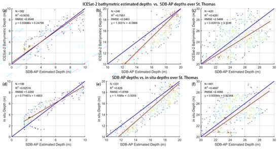
Figure 9.
Error scatter plots in different depth ranges over St. Thomas: (a–c) ICESat-2 bathymetric depths vs. in situ depths; (d–f) SDB-AP depths vs. ICESat-2 bathymetric depths.
Table 2.
Error analysis in different depth ranges: ICESat-2 bathymetric depths vs. SDB-AP depths.
Table 3.
Error analysis in different depth ranges: SDB-AP depths vs. in situ depths.
4.4. Comparison between Adaptive DBSCAN and Standard DBSCAN
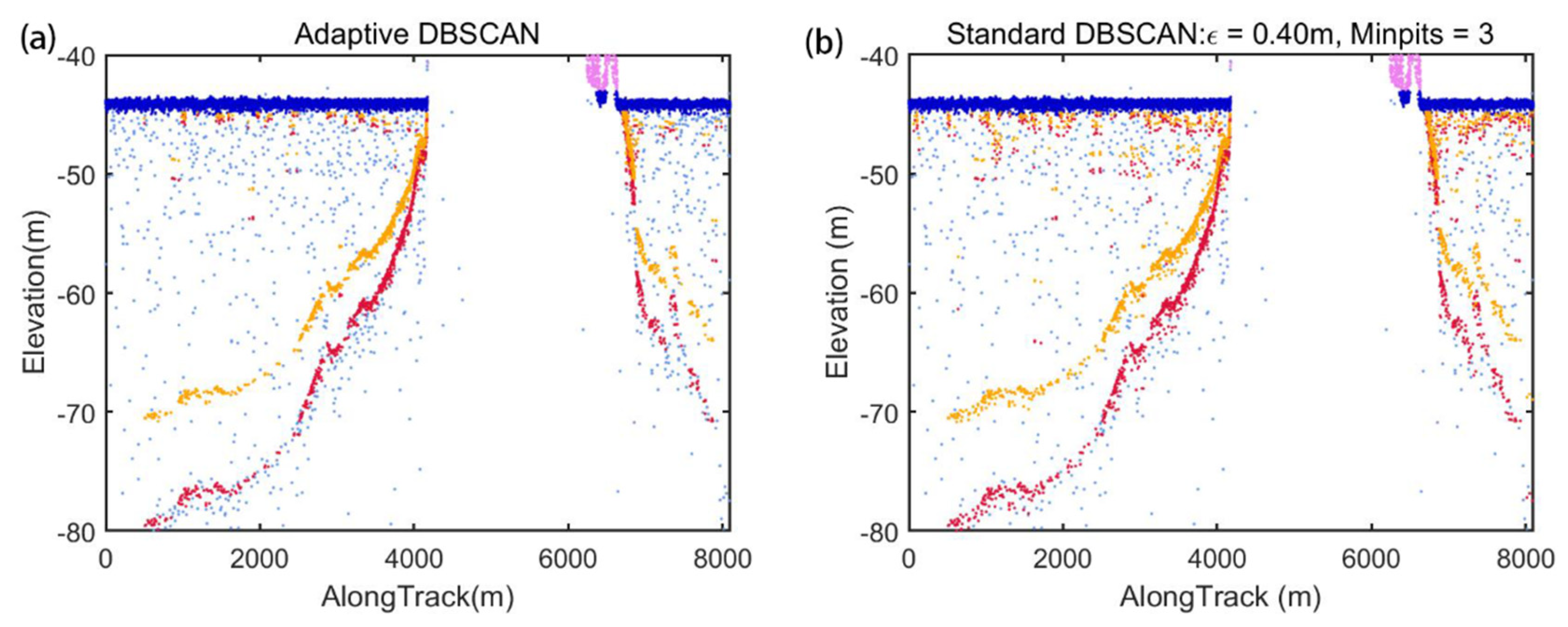
Figure 10a,b shows the results of the detected ICESat-2 signal photons based on our algorithm and the standard DBSCAN algorithm. Retrieval by both methods followed the underwater terrain. However, the result of the standard DBSCAN with fixed and reserved plenty of noisy photons near the sea surface compared with our adaptive DBSCAN algorithm. This may be because the photon density in deep water is much higher than that in shallow water; hence, the DBSCAN with fixed and is suitable for deep water while retaining many noise photons in the high-density sea surface. Figure 11a,b shows the outlier-removal results over the St. Thomas site based on the two methods. The seafloor return photons are light blue, and the outlier-removal signal photons are red. The results showed that our outlier removal algorithm removed most noisy photons near the sea surface, while there were still some outliers by the standard method in Figure 11b, which would reduce water depth estimation accuracy. In Figure 11a, the most outlier photons were clearly eliminated.
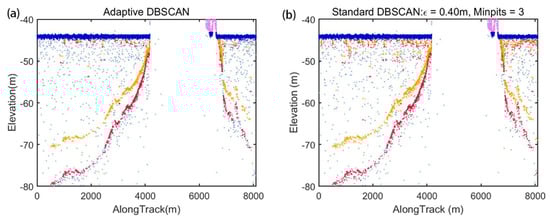
Figure 10.
Comparison of the detected ICESat-2 signal photons based on our method and standard DBSCAN method on 12 December 2020: (a) adaptive DBSCAN; (b) standard DBSCAN with fixed and .
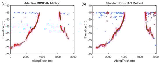
Figure 11.
Outlier removal results over St. Thomas site: the bottom return photons (light blue), the outlier-removal signal photons (red). (a) adaptive DBSCAN; (b) standard DBSCAN with fixed and detection results.
After outlier removal, we used the gridded ICESat-2 bathymetric photon points as model-training data to train the band ration model. Figure A1a,b in Appendix A corresponds to the bathymetric maps derived from the data by our adaptive DBSCAN algorithm and the standard DBSCAN algorithm, respectively. Figure A1c shows the bathymetric map with the in situ data. The dark grey line means the trajectory of ICESat-2 on 13 December 2020 in Figure A1. The trend of the water depth in Figure A1a is consistent with that in Figure A1c. The average water depth found using our method in Figure A1a was 12.68 m, which is close to the in situ with an average depth of 13.98 m in Figure A1c. The estimated water depths in Figure A1b (with an average water depth of 10.22 m) were shallower than the in situ water depths. The derived bathymetric map created using our adaptive DBSCAN algorithm was generally well derived. Moreover, the maximum bathymetric depth in Figure A1b was only 13.25 m, which is far shallower than in situ with 18 m. Figure A2a,b in Appendix A shows the error scatter plots using the two DBSCAN methods over the St. Thomas site. The results derived by our adaptive DBSCAN algorithm showed that the R2 was 0.96 and that the RMSE was 1.14 m, indicating that our algorithm is consistent with the in situ data. However, for the results derived by the standard DBSCAN algorithm, the R2 was 0.94, and the RMSE was 1.94 m.
5. Discussion
5.1. Impact of Outlier Removal on Bathymetry Accuracy
As shown above, although the adaptive DBSCAN algorithm could track the underwater terrain well, there were still some noise photons remaining near the sea surface and seafloor signals. To verify the influence of these noise outliers for overall bathymetry accuracy, we generated the bathymetric maps at the St. Thomas site without outlier removal in Figure A3a in Appendix A. To compare the results, bathymetric maps for the same location obtained from the SDB-AP method and the in situ data were also generated (Figure A3b,c). The estimated water depth in Figure A3a was much shallower than in the other two maps. In addition, it could be noticed that depths in shallow water (2–5 m) were close to the in situ data. The large differences are likely that the outlier photons near sea surface introduce errors for the bathymetry inversion of deep water. Figure A4a–c in Appendix A shows the error scatter plots based on different methods without using the outlier-removal process. They showed that the estimation result stayed away from in situ values without using the outlier removal method, and the RMSEs without outlier removal were 13.90 m, 11.87 m, and 8.73 m, which revealed that the outlier-removal method is significant for SDB.
5.2. Stability of SDB-AP
To verify the stability of our method, we downloaded six Sentinel-2 images on 1 March 2016, 21 November 2016, 21 March 2019, 12 September 2019, 4 April 2020, and 3 May 2021 and retrieved the bathymetric maps over St. Thomas Island using the SDB-AP method. Figure A5a–f in Appendix A shows the six error scatter plots. Over these six dates, the result on 12 September 2019 illustrated the best fitness with in situ data with an R2 of 0.94 and an RMSE of 1.88 m, while the result on 1 March 2016 was relatively the worst, with an R2 of 0.91 and an RMSE of 2.06 m. It should be noted that the deviation between different dates may be caused by many reasons, such as satellite remote-sensing reflection difference or the tide [52,53,54]. For each date, the R2 and RMSEs were also calculated and shown in the top-left corners. The mean R2 was 0.93, and the mean RMSE was 2.00 m, which is less than 10% of the maximum depth. These key regression equation parameters mean great temporal consistency of SDB-AP over different dates.
5.3. Comparison with an Adaptive Variable Ellipse Filtering Bathymetric Method
As we mentioned above, several great DBSCAN algorithms for ICESat-2 photon detection were proposed. For comparison, we selected a similar method named Adaptive Variable Ellipse-Filtering Bathymetric Method (AVEBM) proposed by Chen [32]. AVEBM can precisely identify and separate photons in the above-water, water surface, and water-column regions, and it is based on the characteristics and changes in the density distribution of water-column photons with increasing water depth.
Figure A6a–i in Appendix A shows the ICESat-2 photon detection results based on our adaptive DBSCAN algorithm, AVEBM, and the standard DBSCAN algorithm on 2 February 2019, 24 May 2019, and 19 August 2019. The detected seafloor signal photons are red, the detected sea surface is dark blue, and the noise photons are light blue.
As for the three photons in different regions, the detection results indicated that our adaptive DBSCAN algorithm and the AVEBM could extract seafloor photons accurately. Compared with the other two methods, the standard DBSCAN had the worst detection performance: it ignored minor photons at the end of the underwater topography for low-density data and counted too many background noisy photons for medium- and high-density data.
One of the reasons why our adaptive DBSCAN algorithm could obtain similar results to AVEBM is that we rescaled the current along-track axis according to Equation (2) before density clustering, which increases the detection accuracy of the photon signal using DBSCAN. However, for medium- and high-density photon data, there were still some noise photons remaining along the seafloor signal and sea surface signal in the results from our adaptive DBSCAN. They could be deleted in outlier-removal steps. It was also noticed that there was some small discontinuity in the detected sea-surface signal photons in the results using our adaptive DBSCAN and the AVEBM due to spatial photon distribution change.
5.4. Comparison with Different Methods Deriving Bathymetry from Sentinel-2
In recent research, several approaches have been applied to estimate bathymetry from Sentinel-2, such as extraction wave propagation information or deep learning [55,56]. Deep learning could identify features in satellite images. A deep learning method named Deep Single-Point Estimation of Bathymetry (DSPEB) was proposed [56] and used a convolutional neural network to estimate the average depth of individual local areas. Since this method processes a single small sub-tile at a time, it has demonstrated impressive capabilities for its applicability to many coastal areas. Here, a simple comparison was needed to develop and quantify the performance of classic models and the deep learning method deriving bathymetry from Sentinel-2.
Therefore, we utilized the Neural Clustering tool in MATLAB 2020B to compare the performance of bathymetry estimation of classic models and deep learning. We first defined a 10-layer network. The ICESat-2 corrected seafloor detection results and corresponding above-water surface remote sensing reflectance at the blue and green band from Sentinel-2 images which were used to train the network. The trained network was applied to derive a bathymetric map over the St. Thomas site. Another classic linear model [13] was also applied to generate the bathymetric map over St. Thomas.
Figure A7a,b in Appendix A shows two bathymetric maps derived from Sentinel-2 using the linear model and deep learning method over the St. Thomas site. The maximum bathymetric depths were 31.02 m and 33.23 m in Figure A7a,b. The trend of the linear model results in Figure A7a was similar to that in Figure 6a using the band ratio model, and its average bathymetric depth was 19.23 m. It is clear that the map using the deep learning method presents a deeper bathymetric result in the edges of the selected field with an average depth of 22.88 m.
To compare the performance of the linear band model and deep learning with the band ratio model over St. Thomas, Table 4 and Table A1 in Appendix A list the detailed error analysis in different depth ranges using two methods. Comparing Table 2 and Table A1 in Appendix A, the linear model and the band ratio model had approximate accuracy in the St. Thomas site. In addition, both mathematical models had poor inversion accuracy in deep water. In Table 4, it should be noted the result using the deep learning method had the best bathymetric accuracy in terms of R2. The reason for this may be that the location of points for the error analysis corresponds to the location of points used to train the network. In terms of the RMSE, the deep-learning method had a worse accuracy at 0–10 m, and the reason may be that there were insufficient training points. However, it had better performance in the water depth range of 10 to 30 m. In future research, the deep-learning method is superior for deep-water bathymetry.
Table 4.
Error analysis in different depth ranges: deep learning bathymetric depths vs. in situ depths.
6. Conclusions
In this study, we proposed a satellite-derived bathymetry method by merging active and passive remote sensing in shallow waters and coastal areas. The results showed that the ICESat-2 bathymetric photons reached excellent accuracy with in situ data, and the corresponding RMSE was only 0.99 m. Moreover, the accuracy between the SDB-AP estimated depths and in situ data was also good, and the RMSE was 0.93 m. The RMSEs between the SDB-AP estimated depths and the ICESat-2 bathymetry results over St. Thomas, Acklins Island, and Huaguang Reef were 0.96 m, 0.91 m, and 0.94 m, respectively. This reveals that the SDB-AP method is feasible and efficient. In addition, an adaptive DBSCAN algorithm for raw ICESat-2 photon detection was proposed to adjust the optimal parameters in different underwater topographies. Compared with the standard DBSCAN method, the applied algorithm improved the ICESat-2 bathymetric accuracy and has extended its scope of application. The algorithm showed that the estimation result stays away from in situ values without using the outlier-removal method, revealing that the outlier-removal method is significant for SDB. A suitable outlier removal algorithm was proposed to remove the outlier photons points for the detected ICESat-2 seafloor photons here, which could improve clustering accuracy. The accuracy of SDB-AP was mainly limited to the empirical SDB model error. Further investigation is needed to validate the SDB-AP method in various regions, and the machine learning method is worthy of more investigation for seafloor photon detection and bathymetry retrieval in the future.
Supplementary Materials
The SDB-AP codes and the filtered and corrected ICESat-2 bathymetry tracks are available online at https://github.com/soedchen/SDB/tree/bathymetry-tracks.
Author Contributions
Methodology, C.X.; supervision, P.C.; project Administration, deep learning, P.C.; writing—original draft, C.X.; writing—review & editing, D.P., C.Z. and Z.Z. All authors have read and agreed to the published version of the manuscript.
Funding
This research was funded by the Key Special Project for Introduced Talents Team of Southern Marine Science and Engineering Guangdong Laboratory (GML2019ZD0602); the National Natural Science Foundation (41901305 and 61991453); and the Zhejiang Natural Science Foundation (LQ19D060003), the Scientific Research Fund of the Second Institute of Oceanography, Ministry of Natural Resources (QNYC1803).
Acknowledgments
We thank the anonymous reviewers for their suggestions, which significantly improved the presentation of the paper.
Conflicts of Interest
The authors declare no conflict of interest.
Appendix A
Processing steps of the Adaptive DBSCAN for ICESat-2 Signal Photon Detection are as follows:
S1. Intercepting underwater photons
As mentioned above, ATLAS can collect along-track bathymetric points up to 40 m in depth in very clear water. Before the following processes, the raw ICESat-2 ATL03 data should be intercepted roughly in the vertical direction, including the seafloor, sea surface, and land returns. Its vertical distance range is with [,], where and are the chosen minimum elevation and the maximum elevation, respectively (.
S2. Rescaling the current along-track axis
The along-track spanning distance in this data segment is , and could be described as follows:
where and are the minimum value and the maximum value of the current along-track axis, respectively.
As the order of magnitude and differed greatly, to avoid the calculation error of rounding , the along-track axis is divided times
S3. Dividing the dataset
The ATL03 raw data photon datasets are divided into several segments for processing. Every continuous (usually 5000) points along the along-track direction are a dataset .
S4. Determining the instant sea surface height (SSH)
The “signal_conf_ph” parameters in the ICESat-2 ALT03 data are also introduced. The photons with confidence level of 4 are divided into different bins with a resolution of 0.1 m in the vertical direction. The largest bin would be considered the bin containing the sea surface. We took the median value of this bin as the elevation of sea surface height in the WGS84 ellipsoidal height.
For the sea surface photon accumulation, and are the upper and lower layers of the sea surface photon, respectively. and could be set as follows:
S5. Calculating the average counts of seafloor signal and noise photons
The sea surface photons above are eliminated. The average number of seafloor signal and noise photons is calculated as follows:
where is the number of remaining total photons after eliminating the photons above .
S6. Counting noise-signal-dominated frames
For each dataset, the original photons are divided into frames in the vertical direction, and the height of each frame in the vertical elevation direction is (usually 5 or 10 m). If the number of photons in the photon number in the current frame are bigger than , the current frame is considered as controlling by both noise and signal photons. The photons numbers of these frames are in total, and the number of these vertical frames is .
S7. Counting noise-dominated frames
If the number of photons in the photon number in the current frame is smaller than , the current vertical frame is considered controlled by noise photons. The photons numbers of these frames are in total. The number of these vertical frames is as follows:
S8. Calculating the candidate dataset
The candidate dataset of dataset were obtained as follows:
- Compute the Euclidean distance matrix from to for all points in dataset .
- Sort each row element in the distance matrix in ascending order.The first column of matrix represents the distance from the object to itself and the elements in column constitute the K-nearest neighbor distance vector of all points.
- Calculate the vector mean value . Calculate all to obtain candidate radius dataset , which is expressed as follows:The values of the candidate dataset less than 0.4 would be eliminated.
S9. Calculating the average counts of seafloor signal and noise photons
For each radius , the average number of seafloor signal and noise photon in the circular region is expressed as follows:
where is the area of this circular region with radius . is the number of seafloor signal and noise photons per unit area, and is the reduced along-track spanning distance in this data segment.
S10. Calculating the average counts of noise photons
The average number of noise photons in the circular region with radius was expressed as follows:
where is the number of noise photons per unit area.
S11. Calculating the candidate dataset
As the definition of optimum noise threshold [57], the corresponding to could be expressed as:
where is signal counts, is the noise counts per frame; and is the total mean photoelectron count, equal to the sum of the mean signal and noise counts . The function rounds values to the nearest integer.
S12. Selecting the optimal cluster number
Looping through values: the and with different values are input into the DBSCAN algorithm to cluster the dataset , and the numbers of clusters corresponding to are generated and recorded under different values. When the number of generated clusters are the same three times in succession, the clustering results are judged to be stable, and the current cluster number is the optimal number.
S13. Selecting the optimal value
S12 is repeated until the number of generated clusters is no longer , the maximum value is selected as the optimal value and and are the optimal parameters for DBSCAN. Then, input the optimal parameters into the DBSCAN calculator to calculate the current segment results.
S14. Processing the next data segments
Repeat S4–13 until all data segments are processed.
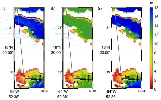
Figure A1.
Sentinel-2 bathymetric maps over the St. Thomas site: (a) our adaptive DBSCAN, (b) standard DBSCAN, (c) in situ. The dark grey line corresponds to the trajectory of ICESat-2 on 13 December 2020.
Figure A1.
Sentinel-2 bathymetric maps over the St. Thomas site: (a) our adaptive DBSCAN, (b) standard DBSCAN, (c) in situ. The dark grey line corresponds to the trajectory of ICESat-2 on 13 December 2020.
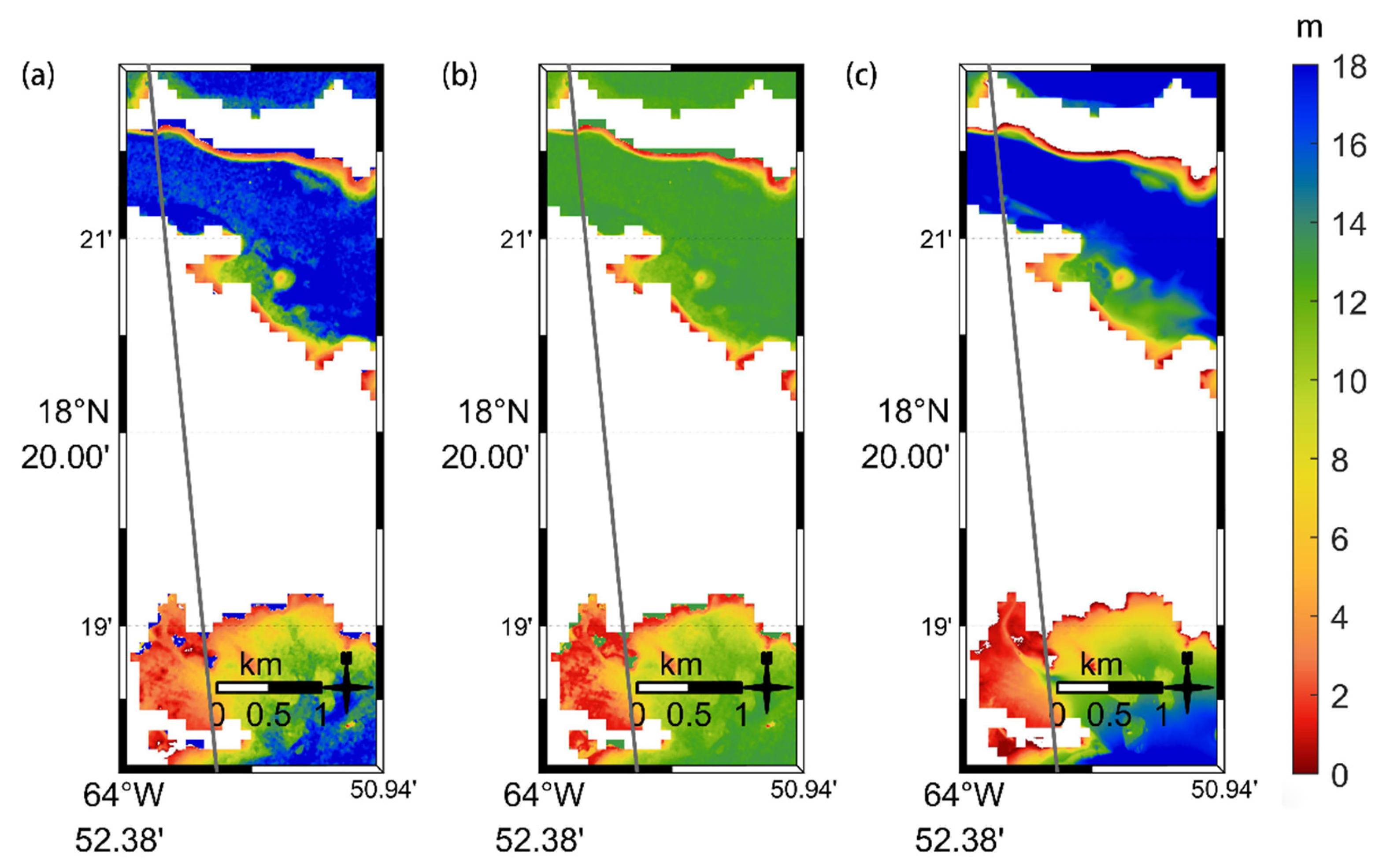
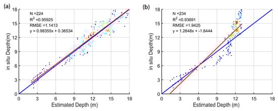
Figure A2.
Error scatter plots near the St. Thomas sites: (a) adaptive DBSCAN; (b) standard DBSCAN. The red line is the 1:1 line, while the blue line represents the regression line. is the number of the training gridded bathymetric points from ICESat-2, and the regression equation details are shown in the top-left corner.
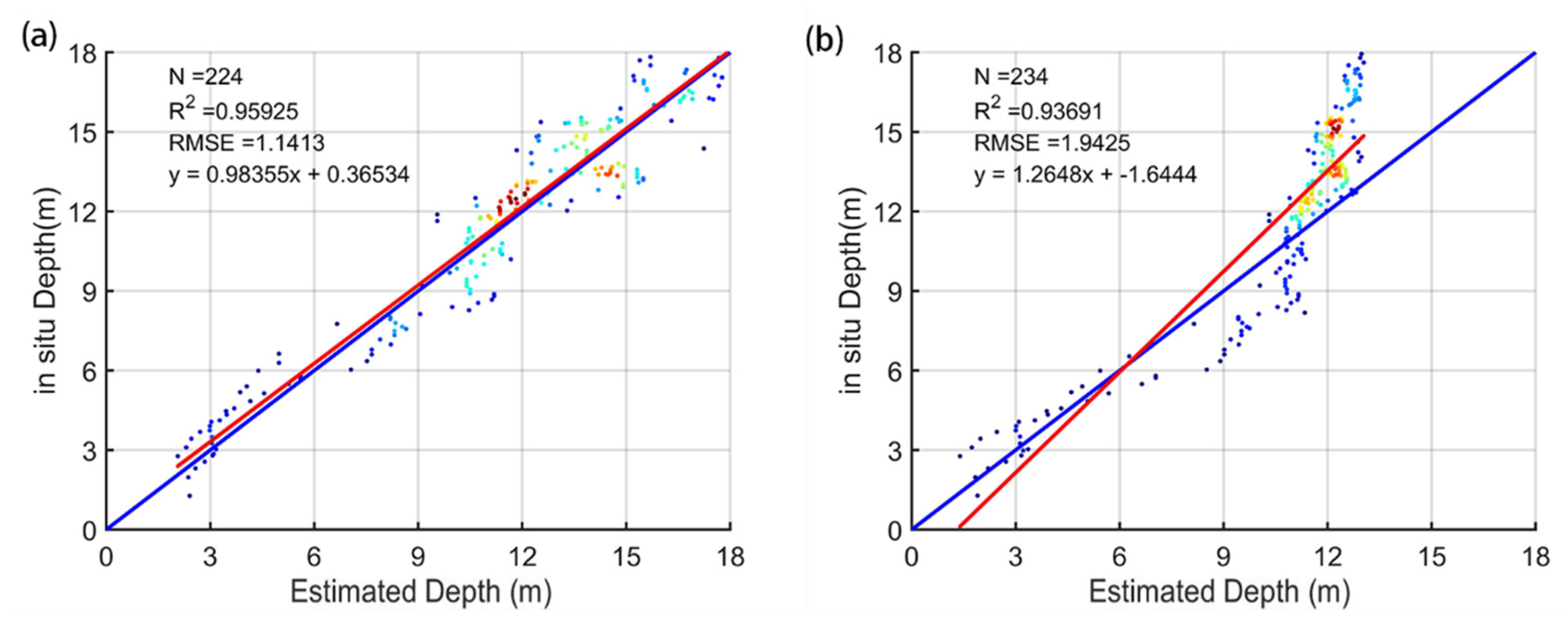

Figure A3.
Bathymetric maps over the St. Thomas site: (a) Sentinel-2 inversion result without outlier removal, (b) Sentinel-2 inversion result with SDB-AP method, (c) in situ data.
Figure A3.
Bathymetric maps over the St. Thomas site: (a) Sentinel-2 inversion result without outlier removal, (b) Sentinel-2 inversion result with SDB-AP method, (c) in situ data.
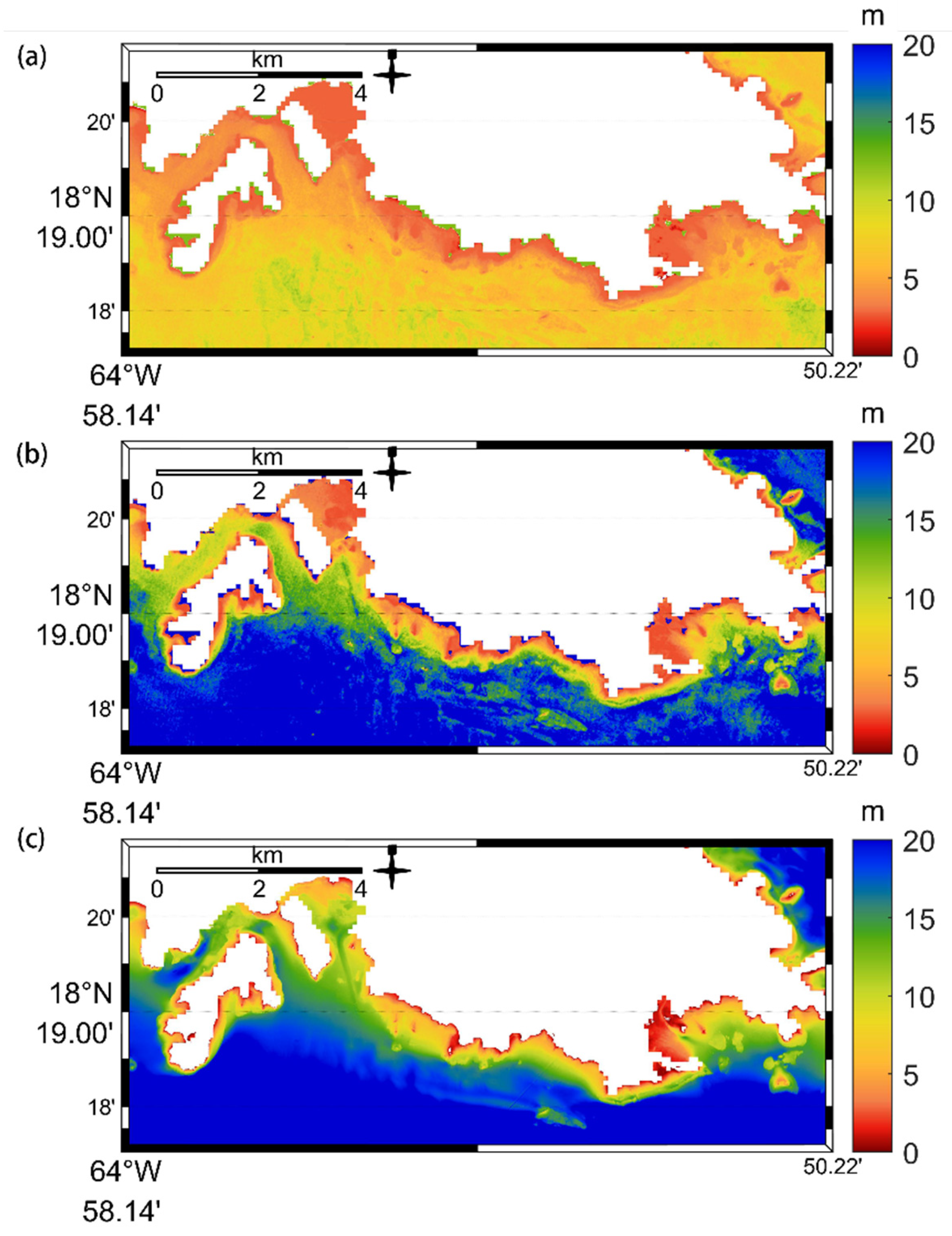
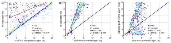
Figure A4.
Error scatter plots for different bathymetry estimation methods over St. Thomas without using the outlier-removal method: (a) ICESat-2 bathymetric estimated depths vs. in situ depths, (b) SDB-AP estimated depths vs. in situ depths, (c) SDB-AP estimated depths vs. ICESat-2 bathymetric estimated depths. The red line is the 1:1 line, while the blue line represents the regression line. is the number of the training gridded bathymetric points from ICESat-2, and the regression equation details are shown in the lower-right corner.

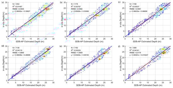
Figure A5.
Error scatter plots on different dates over St. Thomas: (a) 1 March 2016, (b) 21 November 2016, (c) 21 March 2019, (d) 12 September 2019, (e) 4 April 2020, (f) 3 May 2021.
Figure A5.
Error scatter plots on different dates over St. Thomas: (a) 1 March 2016, (b) 21 November 2016, (c) 21 March 2019, (d) 12 September 2019, (e) 4 April 2020, (f) 3 May 2021.
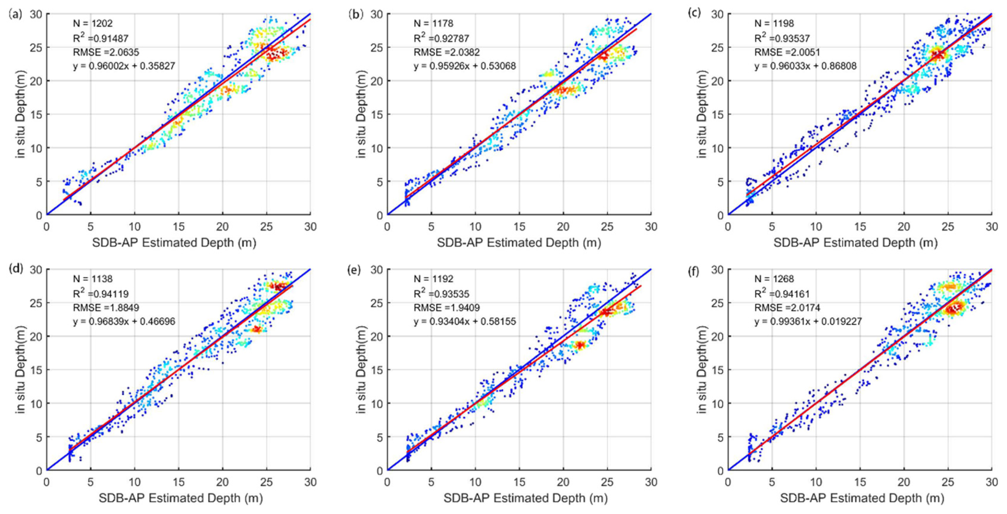
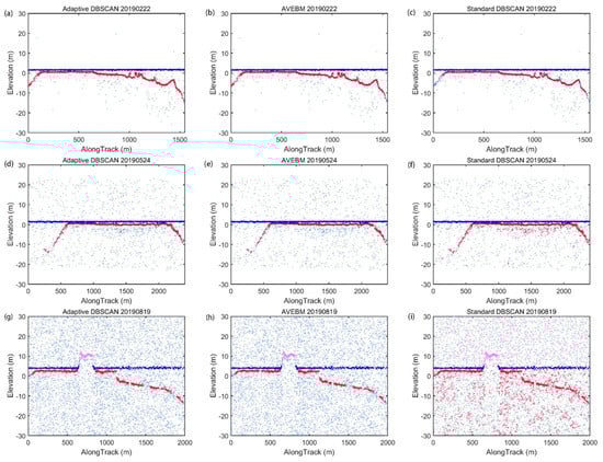
Figure A6.
Comparison of the detected ICESat-2 signal photons based on our method, AVEBM, and the standard DBSCAN method on different dates: (a,d,g) adaptive DBSCAN on 22 February 2019, 24 May 2019, and 19 August 2019, respectively; (b,e,h) AVEBM on 22 February 2019, 24 May 2019, and 19 August 2019, respectively; and (c,f,i) standard DBSCAN with fixed and on 22 February 2019, 24 May 2019, and 19 August 2019, respectively.
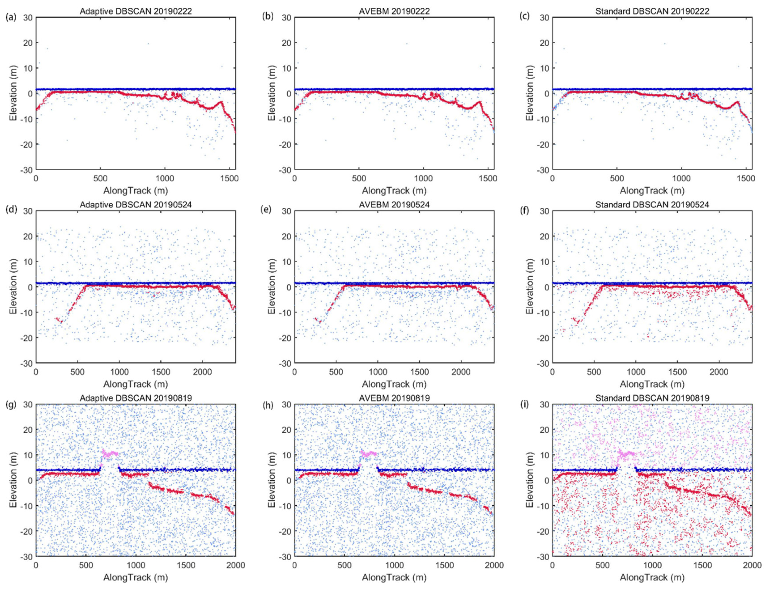
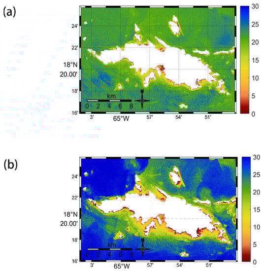
Figure A7.
Bathymetric maps derived from Sentinel-2 using different methods: (a) linear model and (b) deep-learning method.
Figure A7.
Bathymetric maps derived from Sentinel-2 using different methods: (a) linear model and (b) deep-learning method.

Table A1.
Error analysis in different depth ranges: Linear model bathymetric depths vs. in situ depths.
Table A1.
Error analysis in different depth ranges: Linear model bathymetric depths vs. in situ depths.
| Depth (m) | N | R2 | RMSE (m) | Bias (m) | MAE (m) |
|---|---|---|---|---|---|
| 0–10 | 244 | 0.8935 | 1.0700 | −0.1171 | 0.5233 |
| 10–20 | 452 | 0.8125 | 2.6690 | −1.6661 | 2.3869 |
| 20–30 | 541 | 0.4132 | 2.2092 | −0.4535 | 1.8305 |
| 0–30 | 1237 | 0.9225 | 2.0187 | −0.3298 | 1.9875 |
References
- Guenther, G.C.; Brooks, M.W.; LaRocque, P.E. New Capabilities of the “SHOALS” Airborne Lidar Bathymeter. Remote Sens. Environ. 2000, 73, 247–255. [Google Scholar] [CrossRef]
- Trzcinska, K.; Janowski, L.; Nowak, J.; Rucinska-Zjadacz, M.; Kruss, A.; von Deimling, J.S.; Pocwiardowski, P.; Tegowski, J. Spectral features of dual-frequency multibeam echosounder data for benthic habitat mapping. Mar. Geol. 2020, 427, 106239. [Google Scholar] [CrossRef]
- Brown, C.J.; Beaudoin, J.; Brissette, M.; Gazzola, V. Multispectral Multibeam Echo Sounder Backscatter as a Tool for Improved Seafloor Characterization. Geosciences 2019, 9, 126. [Google Scholar] [CrossRef] [Green Version]
- Horta, J.; Pacheco, A.; Moura, D.; Ferreira, O. Can recreational echosounder-chartplotter systems be used to perform accurate nearshore bathymetric surveys? Ocean Dyn. 2014, 64, 1555–1567. [Google Scholar] [CrossRef]
- Saylam, K.; Brown, R.; Hupp, J.R. Assessment of depth and turbidity with airborne Lidar bathymetry and multiband satellite imagery in shallow water bodies of the Alaskan North Slope. Int. J. Appl. Earth Obs. Geoinf. 2017, 58, 191–200. [Google Scholar] [CrossRef]
- William, P. Airborne Laser Hydrography II; American Geophysical Union: Washington, DC, USA, 2019. [Google Scholar]
- Cahalane, C.; Magee, A.; Monteys, X.; Casal, G.; Hanafin, J.; Harris, P. A comparison of Landsat 8, RapidEye and Pleiades products for improving empirical predictions of satellite-derived bathymetry. Remote Sens. Environ. 2019, 233, 111414. [Google Scholar] [CrossRef]
- Watts, A.B.; Tozer, B.; Harper, H.; Boston, B.; Shillington, D.J.; Dunn, R. Evaluation of Shipboard and Satellite-Derived Bathymetry and Gravity Data over Seamounts in the Northwest Pacific Ocean. J. Geophys. Res. Solid Earth 2020, 125, e2020JB020396. [Google Scholar] [CrossRef]
- Behrenfeld, M.J.; Gaube, P.; Della Penna, A.; O’Malley, R.T.; Burt, W.J.; Hu, Y.; Bontempi, P.S.; Steinberg, D.K.; Boss, E.; Siegel, D.A.; et al. Global satellite-observed daily vertical migrations of ocean animals. Nat. Cell Biol. 2019, 576, 257–261. [Google Scholar] [CrossRef]
- Chen, P.; Jamet, C.; Zhang, Z.; He, Y.; Mao, Z.; Pan, D.; Wang, T.; Liu, D.; Yuan, D. Vertical distribution of subsurface phytoplankton layer in South China Sea using airborne lidar. Remote Sens. Environ. 2021, 263, 112567. [Google Scholar] [CrossRef]
- Chen, P.; Mao, Z.; Zhang, Z.; Liu, H.; Pan, D. Detecting subsurface phytoplankton layer in Qiandao Lake using shipborne lidar. Opt. Express 2020, 28, 558–569. [Google Scholar] [CrossRef]
- Salameh, E.; Frappart, F.; Almar, R.; Baptista, P.; Heygster, G.; Lubac, B.; Raucoules, D.; Almeida, L.P.; Bergsma, E.W.J.; Capo, S.; et al. Monitoring Beach Topography and Nearshore Bathymetry Using Spaceborne Remote Sensing: A Review. Remote Sens. 2019, 11, 2212. [Google Scholar] [CrossRef] [Green Version]
- Lyzenga, D.R. Passive remote sensing techniques for mapping water depth and bottom features. Appl. Opt. 1978, 17, 379–383. [Google Scholar] [CrossRef] [PubMed]
- Benny, A.H.; Dawson, G.J. Satellite Imagery as an Aid to Bathymetric Charting in the Red Sea. Cartogr. J. 1983, 20, 5–16. [Google Scholar] [CrossRef]
- Lyzenga, D.R. Shallow-Water bathymetry using combined lidar and passive multispectral scanner data. Int. J. Remote Sens. 1985, 6, 115–125. [Google Scholar] [CrossRef]
- Casal, G.; Monteys, X.; Hedley, J.; Harris, P.; Cahalane, C.; McCarthy, T. Assessment of empirical algorithms for bathymetry extraction using Sentinel-2 data. Int. J. Remote Sens. 2018, 40, 2855–2879. [Google Scholar] [CrossRef]
- Traganos, D.; Poursanidis, D.; Aggarwal, B.; Chrysoulakis, N.; Reinartz, P. Estimating Satellite-Derived Bathymetry (SDB) with the Google Earth Engine and Sentinel-2. Remote Sens. 2018, 10, 859. [Google Scholar] [CrossRef] [Green Version]
- Muzirafuti, A.; Barreca, G.; Crupi, A.; Faina, G.; Paltrinieri, D.; Lanza, S.; Randazzo, G. The Contribution of Multispectral Satellite Image to Shallow Water Bathymetry Mapping on the Coast of Misano Adriatico, Italy. J. Mar. Sci. Eng. 2020, 8, 126. [Google Scholar] [CrossRef] [Green Version]
- Xu, N.; Ma, X.; Ma, Y.; Zhao, P.; Yang, J.; Wang, X.H. Deriving Highly Accurate Shallow Water Bathymetry from Sentinel-2 and ICESat-2 Datasets by a Multitemporal Stacking Method. IEEE J. Sel. Top. Appl. Earth Obs. Remote. Sens. 2021, 14, 6677–6685. [Google Scholar] [CrossRef]
- Gernez, P.; Lafon, V.; Lerouxel, A.; Curti, C.; Lubac, B.; Cerisier, S.; Barillé, L. Toward Sentinel-2 High Resolution Remote Sensing of Suspended Particulate Matter in Very Turbid Waters: SPOT4 (Take5) Experiment in the Loire and Gironde Estuaries. Remote Sens. 2015, 7, 9507–9528. [Google Scholar] [CrossRef] [Green Version]
- Westley, K. Satellite-Derived bathymetry for maritime archaeology: Testing its effectiveness at two ancient harbours in the Eastern Mediterranean. J. Archaeol. Sci. Rep. 2021, 38, 103030. [Google Scholar] [CrossRef]
- Caballero, I.; Stumpf, R. Towards Routine Mapping of Shallow Bathymetry in Environments with Variable Turbidity: Contribution of Sentinel-2A/B Satellites Mission. Remote Sens. 2020, 12, 451. [Google Scholar] [CrossRef] [Green Version]
- Parrish, C.E.; Magruder, L.A.; Neuenschwander, A.L.; Forfinski-Sarkozi, N.; Alonzo, M.; Jasinski, M. Validation of ICESat-2 ATLAS Bathymetry and Analysis of ATLAS’s Bathymetric Mapping Performance. Remote Sens. 2019, 11, 1634. [Google Scholar] [CrossRef] [Green Version]
- Markus, T.; Neumann, T.; Martino, A.; Abdalati, W.; Brunt, K.; Csatho, B.; Farrell, S.; Fricker, H.A.; Gardner, A.; Harding, D.; et al. The Ice, Cloud, and land Elevation Satellite-2 (ICESat-2): Science requirements, concept, and implementation. Remote Sens. Environ. 2017, 190, 260–273. [Google Scholar] [CrossRef]
- Narine, L.; Popescu, S.; Neuenschwander, A.; Zhou, T.; Srinivasan, S.; Harbeck, K. Estimating aboveground biomass and forest canopy cover with simulated ICESat-2 data. Remote Sens. Environ. 2019, 224, 1–11. [Google Scholar] [CrossRef]
- Leigh, H.W.; Magruder, L.A.; Carabajal, C.C.; Saba, J.L.; McGarry, J.F. Development of Onboard Digital Elevation and Relief Databases for ICESat-2. IEEE Trans. Geosci. Remote Sens. 2014, 53, 2011–2020. [Google Scholar] [CrossRef]
- Abdalati, W.; Zwally, H.J.; Bindschadler, R.; Csatho, B.; Farrell, S.; Fricker, H.A.; Harding, D.; Kwok, R.; Lefsky, M.; Markus, T.; et al. The ICESat-2 Laser Altimetry Mission. Proc. IEEE 2010, 98, 735–751. [Google Scholar] [CrossRef]
- Farrell, S.L.; Duncan, K.; Buckley, E.M.; Richter-Menge, J.; Li, R. Mapping Sea Ice Surface Topography in High Fidelity with ICESat-2. Geophys. Res. Lett. 2020, 47, e2020GL090644. [Google Scholar] [CrossRef]
- Farrell, S.L.; Brunt, K.M.; Ruth, J.M.; Kuhn, J.M.; Connor, L.N.; Walsh, K.M. Sea-Ice freeboard retrieval using digital photon-counting laser altimetry. Ann. Glaciol. 2015, 56, 167–174. [Google Scholar] [CrossRef] [Green Version]
- Ma, Y.; Xu, N.; Sun, J.; Wang, X.H.; Yang, F.; Li, S. Estimating water levels and volumes of lakes dated back to the 1980s using Landsat imagery and photon-counting lidar datasets. Remote Sens. Environ. 2019, 232, 111287. [Google Scholar] [CrossRef]
- Forfinski-Sarkozi, N.A.; Parrish, C.E. Analysis of MABEL Bathymetry in Keweenaw Bay and Implications for ICESat-2 ATLAS. Remote Sens. 2016, 8, 772. [Google Scholar] [CrossRef] [Green Version]
- Chen, Y.; Le, Y.; Zhang, D.; Wang, Y.; Qiu, Z.; Wang, L. A photon-counting LiDAR bathymetric method based on adaptive variable ellipse filtering. Remote Sens. Environ. 2021, 256, 112326. [Google Scholar] [CrossRef]
- Thomas, N.; Pertiwi, A.P.; Traganos, D.; Lagomasino, D.; Poursanidis, D.; Moreno, S.; Fatoyinbo, L. Space-Borne Cloud-Native Satellite-Derived Bathymetry (SDB) Models Using ICESat-2 and Sentinel-2. Geophys. Res. Lett. 2021, 48, e2020GL092170. [Google Scholar] [CrossRef]
- Forfinski-Sarkozi, N.A.; Parrish, C.E. Active-Passive Spaceborne Data Fusion for Mapping Nearshore Bathymetry. Photogramm. Eng. Remote Sens. 2019, 85, 281–295. [Google Scholar] [CrossRef]
- Ma, Y.; Xu, N.; Liu, Z.; Yang, B.; Yang, F.; Wang, X.H.; Li, S. Satellite-Derived bathymetry using the ICESat-2 lidar and Sentinel-2 imagery datasets. Remote Sens. Environ. 2020, 250, 112047. [Google Scholar] [CrossRef]
- Albright, A.; Glennie, C. Nearshore Bathymetry from Fusion of Sentinel-2 and ICESat-2 Observations. IEEE Geosci. Remote Sens. Lett. 2021, 18, 900–904. [Google Scholar] [CrossRef]
- Pittman, S.J.; Battista, T.A.; Caldow, C.; Clark, R. Survey and Impact Assessment of Derelict Fish Traps in St. Thomas and St. John; NOAA National Centers for Coastal Ocean Science: Silver Spring, MD, USA, 2012.
- Continuously Updated Digital Elevation Model (CUDEM)—Ninth Arc-Second Resolution Bathymetric-Topographic Tiles. Available online: https://chs.coast.noaa.gov/htdata/raster2/elevation/NCEI_ninth_Topobathy_2014_8483/ (accessed on 20 October 2021).
- ATLAS/ICESat-2 L2A Global Geolocated Photon Data, Version 4. Available online: https://nsidc.org/data/atl03 (accessed on 20 October 2021).
- Altamimi, Z.; Rebischung, P.; Métivier, L.; Collilieux, X. ITRF2014: A new release of the International Terrestrial Reference Frame modeling nonlinear station motions. J. Geophys. Res. Solid Earth 2016, 121, 6109–6131. [Google Scholar] [CrossRef] [Green Version]
- Neumann, T.; Brenner, A.; Hancock, D.; Luthcke, S.; Lee, J.; Robbins, J.; Harbeck, K.; Bae, S.; Brunt, K.; Gibbons, A.; et al. Algorithm Theoretical Basis Document (ATBD) for Global Geolocated Photons ATL03; NASA National Snow and Ice Data Center Distributed Active Archive Center: Boulder, CO, USA, 2018. [Google Scholar]
- Neumann, T.A.; Martino, A.J.; Markus, T.; Bae, S.; Bock, M.R.; Brenner, A.C.; Brunt, K.M.; Cavanaugh, J.; Fernandes, S.T.; Hancock, D.W.; et al. The Ice, Cloud, and Land Elevation Satellite—2 mission: A global geolocated photon product derived from the Advanced Topographic Laser Altimeter System. Remote Sens. Environ. 2019, 233, 111325. [Google Scholar] [CrossRef]
- U.S. Geological Survey. Available online: https://earthexplorer.usgs.gov/ (accessed on 20 October 2021).
- Müller, W. Sen2Cor Software Release Note; European Space Agency: Paris, France, 2018. [Google Scholar]
- Ester, M.; Kriegel, H.P.; Sander, J.; Xu, X. A Density-based Algorithm for Discovering Clusters in Large Spatial Databases with Noise. In Proceedings of the Second International Conference on Knowledge Discovery and Data Mining (KDD-96), Portland, OR, USA, 2–4 August 1996; Volume 34, pp. 226–231. [Google Scholar]
- Ahmed, M.; Naser, A. A novel approach for outlier detection and clustering improvement. In Proceedings of the 2013 IEEE 8th Conference on Industrial Electronics and Applications (ICIEA), Melbourne, VIC, Australia, 19–21 June 2013; pp. 577–582. [Google Scholar] [CrossRef]
- Park, H.-S.; Jun, C.-H. A simple and fast algorithm for K-medoids clustering. Expert Syst. Appl. 2009, 36, 3336–3341. [Google Scholar] [CrossRef]
- Kariya, T.; Sinha, B.K. Detection of Outliers. In Robustness of Statistical Tests; Academic Press: Cambridge, MA, USA, 1989. [Google Scholar]
- Obregón, M.; Rodrigues, G.; Costa, M.J.; Potes, M.; Silva, A.M. Validation of ESA Sentinel-2 L2A Aerosol Optical Thickness and Columnar Water Vapour during 2017–2018. Remote Sens. 2019, 11, 1649. [Google Scholar] [CrossRef] [Green Version]
- SNAP Supported Plugins Sen2Cor. Available online: http://step.esa.int/main/snap-supported-plugins/sen2cor/ (accessed on 20 October 2021).
- Louis, J.; Debaecker, V.; Pflug, B.; Main-Knorn, M.; Bieniarz, J.; Mueller-Wilm, U.; Cadau, E.; Gascon, F. SENTINEL-2 SEN2COR: L2A Processor for Users. In Proceedings of the Living Planet Symposium 2016, Prague, Czech Republic, 9–13 May 2016; pp. 1–8. [Google Scholar]
- Caballero, I.; Stumpf, R.P. Retrieval of nearshore bathymetry from Sentinel-2A and 2B satellites in South Florida coastal waters. Estuar. Coast. Shelf Sci. 2019, 226, 106277. [Google Scholar] [CrossRef]
- Casal, G.; Harris, P.; Monteys, X.; Hedley, J.; Cahalane, C.; McCarthy, T. Understanding satellite-derived bathymetry using Sentinel 2 imagery and spatial prediction models. GIScience Remote Sens. 2019, 57, 271–286. [Google Scholar] [CrossRef]
- Vahtmäe, E.; Kutser, T. Airborne mapping of shallow water bathymetry in the optically complex waters of the Baltic Sea. J. Appl. Remote Sens. 2016, 10, 25012. [Google Scholar] [CrossRef]
- Bergsma, E.W.; Almar, R.; Rolland, A.; Binet, R.; Brodie, K.L.; Bak, A.S. Coastal morphology from space: A showcase of monitoring the topography-bathymetry continuum. Remote Sens. Environ. 2021, 261, 112469. [Google Scholar] [CrossRef]
- Al Najar, M.; Thoumyre, G.; Bergsma, E.W.J.; Almar, R.; Benshila, R.; Wilson, D.G. Satellite derived bathymetry using deep learning. Mach. Learn. 2021, 1–24. [Google Scholar] [CrossRef]
- Degnan, J.J. Photon-Counting multikilohertz microlaser altimeters for airborne and spaceborne topographic measurements. J. Geodyn. 2002, 34, 503–549. [Google Scholar] [CrossRef] [Green Version]


Publisher’s Note: MDPI stays neutral with regard to jurisdictional claims in published maps and institutional affiliations. |
© 2021 by the authors. Licensee MDPI, Basel, Switzerland. This article is an open access article distributed under the terms and conditions of the Creative Commons Attribution (CC BY) license (https://creativecommons.org/licenses/by/4.0/).