Letter

Sea Surface Wind Speed Retrieval from the First Chinese GNSS-R Mission: Technique and Preliminary Results

1
China Academy of Space Technology (Xi’an), Xi’an 710101, China
2
State Key Laboratory of Remote Sensing Science, Aerospace Information Research Institute, Chinese Academy of Sciences, Beijing 100101, China
3
School of Information and Electronics, Beijing Institute of Technology, Beijing 100081, China
4
National Key Laboratory of Science and Technology and Space Microwaves, Xi’an 100101, China
5
National Satellite Meteorological Center, China Meteorological Administration, Beijing 100081, China
6
DFH Satellite Co. Ltd., Beijing 100094, China
7
Hainan Key Laboratory of Earth Observation, Sanya 572029, China
*
Author to whom correspondence should be addressed.
Remote Sens. 2019, 11(24), 3013; https://doi.org/10.3390/rs11243013
Submission received: 30 October 2019 / Revised: 10 December 2019 / Accepted: 12 December 2019 / Published: 14 December 2019

Abstract

:
Launched on 5 June 2019, the BuFeng-1 A/B twin satellites were part of the first Chinese global navigation satellite system reflectometry (GNSS-R) satellite mission. In this letter, a brief introduction of the BF-1 mission and its preliminary results of sea surface wind retrieval are presented. Empirical fully developed sea (FDS) geophysical model functions (GMFs) relating the normalized bistatic radar cross-section to the sea surface wind speed are proposed for the BF-1 GNSS-R instruments. The FDS GMFs are derived from the collocated BF-1 observations, the European Center for Medium-Range Weather Forecasts (ECMWF) reanalysis data, and the advanced scatterometer (ASCAT) satellite observations. The preliminary tests reveal that the root-mean-square error (RMSE) between the derived wind speed and the reanalysis is 2.63 m/s for wind speeds in the range of 0.5–40.5 m/s. Further comparisons with the ASCAT observations and mooring buoys show that the RMSEs are 2.04 m/s and 1.77 m/s, respectively, at low-to-moderate wind speeds. This study demonstrates the effectiveness of BF-1 and provides a basis for the future GMF development of the BF-1 A/B mission.

1. Introduction

The global navigation satellite system (GNSS) continuously emits L-band microwaves to the Earth’s surface, which are then reflected into space. By using a GNSS-reflectometry (GNSS-R) receiver, the Earth-reflected signals carrying geophysical information can be collected. In 1988, this GNSS-R technique was first applied to ocean scatterometry [1]. In 1993, Martin-Neira [2] proposed the PAssive Reflectometry and Interferometry System (PARIS) concept to use the reflected GPS signal to perform ocean altimetry. After this, GNSS-R signals were received on land-based, coastal, and airborne platforms to prove the sufficient power budget [3,4,5,6,7,8,9,10,11,12,13]. Then, this technique was first tested in orbit by the UK-Disaster Monitoring Constellation (UK-DMC) mission in 2003 [14,15]. The first delay Doppler map (DDM) from low Earth orbit was obtained by this mission. In July 2014, a technology demonstration GNSS-R satellite, TechDemoSat-1 (TDS-1), was launched and served for 4.5 years. The onboard GNSS-R receiver, SGR-ReSI, collected a lot of valuable in-orbit data, including sea surface winds, sea surface height, inland soil moisture, and sea ice [16,17,18,19,20,21]. The results of TDS-1 provide a strong support for future GNSS-R operational running of global wind speed retrieval. On 17 December 2016, NASA launched eight microsatellites to establish a constellation for observing tropical cyclones (TCs) with a high spatial–temporal resolution. The NASA Cyclone GNSS (CYGNSS) mission has demonstrated the capability of the GNSS-R technique to sense the TC eyes in high temporal resolution, optimize TC forecasts, supply monthly high-resolution soil moisture products, and map inland waterways [22,23,24,25,26].
Regarding the sea surface wind speed retrieval, approaches have experienced three stages. The first is based on the theory of the scattering model proposed by Zavorotny and Voronovich in 2000 [3]. This theoretical model can simulate different sea state waveforms of GNSS-reflected signals so that wind speeds can be inversed by the delay waveform matching method [4,5,6,7,8]. The second stage focuses on the observables abstracted from the DDMs that are the standard product of airborne and spaceborne GNSS-R receivers. The observable DDM average (DDMA) directly relates to the sea surface roughness [27,28,29]. The third stage uses the normalized bistatic radar cross section (NBRCS), also known as the scattering coefficient, as an indicator to retrieve the sea surface wind speed [30]. The NBRCS calculation method has been proposed and improved in recent years [31,32,33,34]. Combined with power calibration, the NBRCS can be calculated more accurately; therefore, it can agree well with the full sea surface wind speed range. The NBRCS is one of the two observables that produce the global tropical cyclone satellite product of the NASA CYGNSS constellation [23].
Typhoons are one of the most destructive natural disasters in China. Satellite remote sensing can provide near-real-time observations of typhoon tracks and intensities, which has become an indispensable part of typhoon monitoring and forecasting [35,36,37,38,39]. After recent years of research, the use of GNSS-R constellations to sense the sea surface roughness has been deemed a more effective and less costly method. On 5 June 2019, the first two Chinese GNSS-R satellites, BF-1 A/B, were launched into low Earth orbit (LEO) by the LongMarch 11 rocket at a sea launch platform as demonstration satellites for typhoon GNSS-R observations. Afterwards, following UK, US, and Japan, China became the fourth country that has GNSS-R satellites in Earth orbit. At the same time, BF-1 A/B is the only two-GNSS-R constellation in the world. The world’s first spaceborne BDS DDM is also mapped in this mission.
The next section provides an overview of the first Chinese GNSS-R mission, as well as a large amount of GNSS-R data collected from the global ocean surface in July and August 2019. In Section 3, new geophysical model functions (GMFs) for fully developed seas (FDSs) are proposed to derive the sea surface wind speed from the BF-1 NBRCS. Section 4 describes the preliminary retrieval and validation results for the sea surface wind speed, which are excellent for both the wind speed range and the accuracy compared with current GNSS-R missions. Section 5 summarizes the conclusions.

2. Places, Instruments, and Data

2.1. Places

The places studied are limited by orbital configurations. The BF-1 A/B satellites operate at altitudes of 579 km with an orbital inclination of 45°. In fact, within the antenna footprint, the specular points are scattered from latitudes 53°S to 53°N, as shown in Figure 1. This area can cover most of the typhoon events [24] and coastal lines of China. The other study area is also shown in Figure 1 of the central equatorial Pacific Ocean, where the red diamonds are the 55 mooring buoys deployed by the Tropical Atmosphere Ocean (TAO) program of the National Data Buoy Center (NDBC).

2.2. BF-1 Mission and Instruments

“Bu Feng (捕风)” means “chasing the winds” in Chinese; BF-1 A/B is the first Chinese GNSS-R mission comprising two demonstration satellites. The payloads of the BF-1 A/B twin satellites, which are the main payloads of the carrier, were developed by the China Aerospace Science and Technology Corporation (CASC). Each platform has two nadir GNSS-R antennas, one navigation antenna, one auxiliary antenna, four low-noise amplifiers with blackbody calibration, and a GNSS-R receiver. The two nadir antennas are directed at the left and right sides of the platform with inclination angles of 26°. In general, the number of specular points located in the antenna footprint of the Global Positioning system (GPS) is approximately four. Both the instruments have four digital channels to receive the best four signals out of the specular points by different GNSS satellites. For every second, the onboard receivers can simultaneously process the four reflected signals into DDMs. The specifications of the receiver are shown in Table 1.
Each GNSS-R receiver collects four DDMs per second for 24 h each day. In this mission, the world’s first in-orbit BDS DDM was mapped on 10 June 2019 and its first DDM was acquired on 9 June 2019. The in-orbit-measured DDM has dimensions of 128 × 21, corresponding to 32 delay chips in quarter chip increments and a 5000 Hz Doppler frequency with 250 Hz intervals. Examples of DDMs measured by the BF-1A instrument are shown in Figure 2.

2.3. Data

To develop the FDS GMF and test its performance, we introduced three datasets: buoy measurements, satellite scatterometer observations, and European Center for Medium-Range Weather Forecasts (ECMWF) reanalysis data.

2.3.1. Buoy Measurements

The TAO buoy array was obtained from the NDBC, supported primarily by the US National Oceanic and Atmospheric Administration (NOAA). The TAO array comprises 55 moored buoys near the central equatorial Pacific Ocean. It is a sensor network telemetering oceanographic and metrological data in real-time by taking the advantage of the Argos satellite system. Therefore, the measured sea surface winds are appropriate for the instant performance assessment at low and moderate wind speeds.
The NDBC TAO measurements mainly include surface winds, sea surface temperature, ocean currents, precipitation, humidity, salinity, and pressure. Figure 1 shows the distribution of the mooring buoys we used: they are arranged in eight columns from 165°E to 95°W longitudes and 8°S to 9°N latitudes. The temporal resolution is 10 min. The real-time data have a 1-h delay of obtainment and the historic data has a lag of one day. For the wind speed measurements, the NOAA NDBC buoy data have an accuracy of 1.0 m/s or 10%, which is the highest accuracy among the three datasets in this paper.
The wind from the TAO program is at a 4-m reference height, which can be calibrated into the standard U10 by the following equation [40]:
U10 = Uz8.87403/ln(z/0.0016),
where z (m) is the observation height, Uz is the wind speed at the observation height, and U10 is the 10-m reference height wind speed.

2.3.2. ASCAT Observations

The advanced scatterometer (ASCAT) is a C-band active microwave instrument on the EUMETSAT MetOp satellites, operating since 2007. ASCAT measures the sea surface roughness, which relates to wind speeds 10 m above the water’s surface. In this study, we used the ASCAT version 2.1 data, which are reprocessed by the remote sensing systems (RSSs) with the latest GMF, C-2015 [41]. The RSS produces daily wind field products with a spatial resolution of 25 km in the form of ascending and descending swaths. ASCAT winds are known as being reprocessed with high accuracy. Compared with mooring buoys, unbiased global ASCAT wind errors on the scatterometer measurement scale are about 0.7 m/s [42].

2.3.3. ECMWF Reanalysis Data

The ECMWF supplies both global numerical weather predictions (NWPs) and reanalysis history datasets of the atmosphere, land surface, and oceans. The ECMWF reanalysis data are based on the integrated forecast model and provide spatially continuous wind products globally with an interpolated spatial resolution of up to 0.125° longitude/latitude and a temporal resolution of 3 h. Two reanalysis datasets are available for sea surface winds until 1 September 2019: ERA-Interim and ERA5.

3. Methodology

3.1. Delay Doppler Maps (DDMs)

DDMs are the standard products of spaceborne GNSS-R, as shown in Figure 2. The DDM instruments (DDMI) onboard BF-1 A/B create the DDMs by receiving the sea surface-reflected GNSS signal powers in every time delay and the Doppler frequency bins. Similarly, the instruments use a 1-ms coherent integration time and 1000-times noncoherent integration to guarantee the signal-to-noise ratio (SNR). The theoretical DDM calculations are described by Zavorotny-Voronovich [3] as follows:
| Y ( τ , f ) | 2 = P t G t λ 2 T i 2 ( 4 π ) 3 A G r σ 0 Λ 2 ( τ ) S 2 ( f ) R t 2 R r 2 d A ,
where | Υ ( τ , f ) | 2 is the correlation power of each code delay (τ) and Doppler frequency (f) in every DDM bin, Pt is the transmitter power, Gt is the transmitter antenna gain, λ is the L-band wavelength of ~19 cm for the GPS L1 carrier, Ti is the coherent integration time, Gr is the receiver antenna gain, Λ2(τ) is the delay code auto-relation function, S2(f) is the Doppler frequency function, A is the effective area of the certain code delay and Doppler frequency, Rt and Rr are the distances of the effective area to the transmitter and receiver, respectively, σ 0 is the scattering parameter sensitive to the sea surface roughness, which highly correlates with the sea surface wind speed. Once the σ 0 is determined, the DDM can be simulated by Equation (2).

3.2. NBRCS Calculation

The parameter σ 0 mentioned in Equation (2) above is also the NBRCS. In this study, the NBRCS is applied as the sea surface roughness-sensitive parameter, also known as the observable, to retrieve the sea surface wind speeds [30]. To calculate the NBRCS ( σ 0 ), Equation (2) can be rewritten as follows [33]:
σ 0 , τ , f = P τ , f g ( 4 π ) 3 R t 2 R r 2 P t λ 2 G t G r / A Λ 2 ( τ ) S 2 ( f ) d A ,
where most of the terms are the same as those in Equation (2), however, P τ , f g is the power calibration result of | Υ ( τ , f ) | 2 , and Rt and Rr are the specular distances to the transmitter and receiver, respectively. These two range loss terms from the integration are based on the assumption that the ranges are approximately equal near the specular point. Because the averaged NBRCS used to retrieve the winds is only a small area around the specular point, the uncertainty of this assumption regarding the range loss is nearly negligible.
It should be noted that the content in the double integration of Equation (3) is determined only by the geometry. Once the positions and velocities of the receiver and transmitter are determined, the specular point can be calculated numerically. Then, a grid is built around the specular point to compute the contributions in each delay and the Doppler frequency bin. As the other geometry terms, like the antenna gains and range losses, are not considered integrally, σ 0 only has good accuracy near the specular point. Therefore, a 1.5-chip and 2000-Hz delay Doppler domain was selected to calculate the NBRCS ( σ 0 ) in this study, which can also be considered as the DDMA.

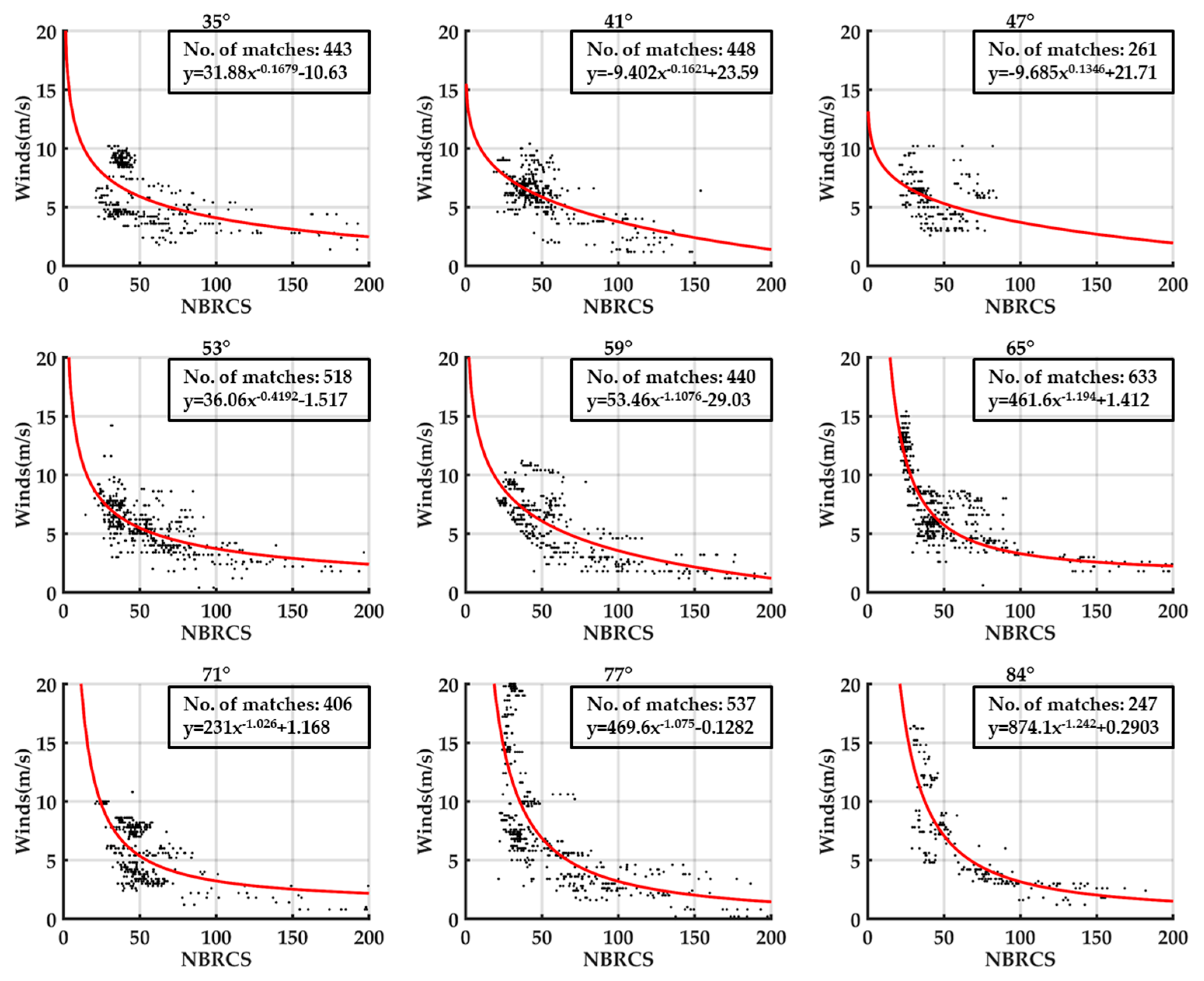
3.3. FDS GMF Development

In this subsection, the ECMWF reanalysis data and ASCAT observations from 1 July 2019 to 1 September 2019 are used as training datasets to develop FDS GMFs. The reanalysis data can supply a spatially continuous wider wind speed range corresponding to a larger amount of matchup pairs. On the other hand, the ASCAT observations have a higher accuracy on wind speed and limited swaths which result in less collocated winds.

3.3.1. ECMWF Reanalysis Data

The matchup NWP data, used to train the empirical FDS GMF, are the 10-m referenced sea surface wind speed reanalysis data provided by the ECMWF. In this study, we used the ERA-Interim dataset of the ECMWF reanalysis to conduct a 2-month global sea surface wind speed retrieval from 1 July 2019 to 1 September 2019. The ERA-Interim reanalysis dataset used has an interpolated spatial dimension of 0.125° longitude/latitude and 3-h increments of temporal resolution. Finally, the matchup volume of the NBRCSs was 12,632,225 with alignment criteria of 1 h and the nearest longitude/latitude grid. The matchup maximum wind was up to 40.8 m/s.
After the 3-dB beam-width antenna pattern screening, the scatter density plot was obtained between the NBRCS and ECMWF reanalysis winds, as shown in Figure 3a. The wind speeds range from 0.5 to 40.8 m/s. A significant power function relationship between the ECMWF reanalysis winds and NBRCS extracted from DDMs can be inferred. Therefore, the empirical FDS GMF was developed based on this relationship. As shown in Figure 3a, 16.86% of the NBRCSs from 0 to 20 correspond to the moderate wind speeds of 5 to 15 m/s, indicating that a large amount of NBRCSs will correspond to this wind speed range. Consequently, the wind speeds above 15 m/s will be underrated by these extra data. Accordingly, a quality control method is necessary to screen out the low NBRCSs that relate to the low and moderate wind speeds mentioned above.
Therefore, after the antenna pattern gains control of a 3-dB beam-width and SNR of 4-dB quality control, 80% of the data were employed as the training set; the remaining 20% was used to validate the model accuracy. The scatter density plot after quality control of the antenna pattern and SNR is shown in Figure 3b. Notably, by setting up the filters of the antenna gain control and SNR threshold, the NBRCS ambiguity problem of moderate wind speeds between 5 and 15 m/s can be largely mitigated from the rate of 16.86% to 1.59%, which effectively improves the performance of the empirical GMF.
Next, we further developed the empirical FDS GMF based on the NBRCS ( σ 0 ), wind speed (U10), and elevation angle (θele). Here, the elevation angle is the angle between the horizontal plane and the line extending from the spacecraft to the specular point. First, we built a lookup table (LUT) for the elevation angle. It is known that the common sea Fresnel coefficient varies as the elevation angle increases. The elevation angle of 28° is the inflection point at which the left-handed circle polarization takes a larger portion compared with the right-handed circle polarization. Thus, the elevation angle is divided into 63 bins, and the bin center is incremented by 1° from 28° to 90° with a 1° bin width. Therefore, all the DDMs and auxiliary information within each elevation bin compute the optimal coefficients of the power function ( U 10 = A σ 0 B + C ), as shown in Figure 4. The coefficients of the power functions of different elevation angles then fill the 2-D LUT. Figure 4 presents examples of the empirical GMF that correspond to elevation angles of 35–84°, indicating that the elevation angle has a greater influence on the wind speed.

3.3.2. ASCAT Data

Using the same process, the ASCAT data were collocated with the BF-1 A/B NBRCS data from 1 July to 1 September. The total number is 860,859 with the matchup criteria of 1 h and the nearest longitude/latitude grid. The reason for the lower volume of coincident pairs is that the ASCAT data are limited by their swath and orbit, which are different from the spatially continuous ECMWF models. The matchup maximum wind speed is 33.2 m/s.
After the same quality control method of the 3-dB antenna beam-width and SNR ≥ 4, 80% of the data were used to train the FDS GMF for the sea surface wind speed. The elevation angle bins remained as 28–90° with a 1° bin width. Figure 5 shows examples of the best-fitted results using the ASCAT training dataset.

4. Wind Retrieval Testing

This section describes the validation of the trained empirical FDS GMFs by three datasets: the remaining 20% collocated reanalysis winds, the remaining 20% of the ASCAT observations validation dataset, and the NDBC TAO mooring buoys measurements.

4.1. Reanalysis Comparisons

When developing the empirical FDS GMF using the reanalysis data, we only used 80% of the matchup data to tune the model coefficients, while the remaining 20% were used for model testing. The remaining 20% was comprised of 461,932 data points. The aligned ECMWF reanalysis wind speeds and NBRCS derived wind speeds are from 0.6 to 36.7 m/s. As shown in Figure 6, most of the data are located around the 1:1 line. The retrieved wind speeds had a root mean square error (RMSE) of 2.72 m/s and the coefficient of determination was 0.5.
Owing to the large number of reanalysis data pairs, another test of 10 minus the alignment criteria was conducted. The total number of matchup pairs then became 428,832. After the 80% training and 20% validation, the scatter density plot was obtained, as shown in Figure 6b. Finally, the unbiased RMSE was 2.63 m/s, and the coefficient of determination was 0.55.

4.2. ASCAT Comparisons

The remaining 20% of the aligned data were applied by the FDS GMF as described in Section 3.3.2. After the quality control filters, the maximum wind speed was 25 m/s and the number of validation data became 34,029. The performance of the ASCAT-trained GMF has an unbiased RMSE of 2.04 m/s, and the coefficient of determination is 0.61, as shown in Figure 7.

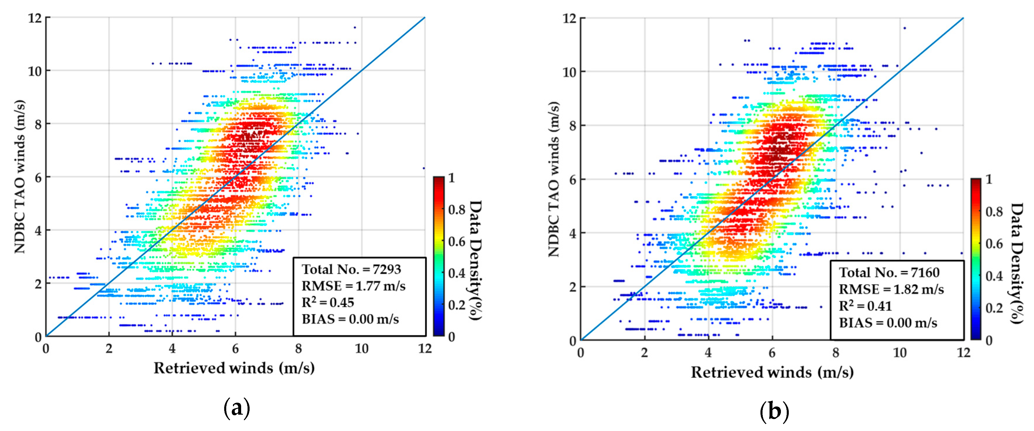
4.3. Buoy Comparisons

Applied using the alignment criteria of 1° longitude/latitude and 10 min, the total number of matchups was 16,552 after the simple antenna 3-dB beam-width quality control. This quantity is insufficient for generating an FDS GMF with multiple elevation bins. Therefore, the NDBC TAO buoy measurements were introduced to validate the robustness of the model functions.
The sea surface wind speeds derived by the proposed empirical FDS GMFs were compared with the NDBC TAO buoy measurements. After a reference transition from 4 m to 10 m, the buoy wind speed measurements were 0.2–11.6 m/s. As shown in Figure 8, compared with the buoy measurements, the reanalysis GMF-derived unbiased RMSE is 1.77 m/s and the coefficient of determination is 0.45. Meanwhile, the ASCAT-derived GMF has an unbiased RMSE of 1.82 m/s and a coefficient of determination of 0.41.

5. Summary and Conclusions

From the process of developing the empirical FDS GMF for the BF-1 A/B twin satellites, some details, such as the effects of the antenna gain control, elevation angle, inconsistency between satellite channels, and SNR, can be further summarized as follows.
The BF-1 A/B DDMs were collected by ranking the antenna gains to the specular points scattered in the antenna footprint. The strongest four antenna gains were selected to be considered closest to the main lobe of the nadir antennas. Without any quality control strategy, the original data had an RMSE above 4 m/s. As Figure 3a illustrates, the percentage of the NBRCS was large at the values between 0 and 20, corresponding to the wind speed range of 5–15 m/s. Consequently, a large portion of the NBRCSs corresponded to this range, so high wind speeds above 15 m/s will be underrated. Therefore, we next explored the following four steps to alleviate this issue. First, a 3-dB half beam-width filter was introduced to ensure the signal is near the main lobe. Thus, the performance of the retrieved wind speed had an RMSE of below 3.8 m/s. Second, the influence of the elevation angle was considered in the GMF by building 63 bins from 28–90°, providing an accuracy of approximately 3.6 m/s of RMSE. Then, the inconsistency between the satellites and channels was considered. As a result, the RMSE became 3.5 m/s. Finally, the most effective factor, SNR, was found to improve the problem of the NBRCS ambiguity between 0 and 20, as illustrated in Figure 3a. After an SNR ≥ 4-dB filter, the percentage of NBRCS ambiguity became 1.59% from 16.86%. Figure 6 shows that the final reanalysis FDS GMF performance has an RMSE of 2.63 m/s at 32.6 m/s, and 2.04 m/s (RMSE) and 0.61 (R2) against the ASCAT observations, as in Figure 7. Thus, regarding the wind speed accuracy and wind speed range, BF-1 performs better than the existing GNSS-R missions: the RMSE of UK TDS-1 against ASCAT is 2.21 m/s for winds between 3 and 18 m/s [19], and the RMSE of CYGNSS FDS GMF is ~4 m/s at 20 m/s, compared with the model reanalysis products [23].
The empirical GMFs were also tested with in-situ buoy measurements. The comparison results show a preliminary agreement at the low-to-moderate wind speed range. The RMSEs of the retrieved wind speeds were 1.77 m/s and 1.82 m/s. Figure 8 provides a clear underestimation of the wind speeds. There are two reasons for this: one is the inconsistency of the ECMWF reanalysis wind data, ASCAT observations, and NDBC TAO buoy wind measurements. Meanwhile, the empirical GMFs were not developed based on the buoy measurements, so the behavior is less impressive than the reanalysis and ASCAT results.
This paper presents the results of sea surface wind speed retrieval using the first Chinese GNSS-R satellite data collected by BF-1 A/B. After months of in-orbit operation, the data were first referenced with the sea surface wind speeds product of the ECMWF reanalysis and ASCAT observations to train the empirical FDS GMFs. The NBRCS extracted from the collected DDM was used as the observable when developing the GMF. Based on the data filter of the 3-dB half-beam-width antenna and SNR ≥ 4 dB, the empirical GMFs were developed using the power function of the NBRCS ( σ 0 ), wind speed (U10), and elevation angle (θele). Then, the validation datasets were applied by the empirical GMFs to derive the global sea surface wind speeds to assess the model accuracy. Even without potentially large platform attitude error corrections, the proposed GMF obtained an unbiased RMSE of 2.63 m/s at wind speeds of 32.7 m/s. The comparison results of the buoy measurements and ASCAT observations show a better performance under low-to-moderate wind speed conditions.
This study provides an important foundation for the construction of future Chinese operational GNSS-R constellations for the observation of typhoons. A GNSS-R constellation can largely increase the capability of the spatial and temporal coverage, thereby enabling near-real-time typhoon observations and forecasts. Furthermore, all objectives mentioned above could be realized by the low-cost GNSS-R technique. However, the forerunner BF-1 A/B twin satellites still require further work. In the future, the attitude information should be studied and introduced to optimize the quality control process. This would definitively improve the performance of the empirical GMF on sea surface wind speed retrieval. Moreover, a study on the sea surface wind speed under heavy precipitation is required to improve the NBRCS behavior for high wind speeds. Finally, assessment of other applications is required for the validation, such as the inland performance to guide the future constellation mission design.

Author Contributions

Conceptualization, C.J., X.N., C.D., F.L., and G.D.; methodology, C.J., X.N., and F.L.; software, C.J. and F.L.; validation, C.J.; formal analysis, C.J.; investigation, C.J. and F.L.; resources, C.J., X.N.; data curation, C.J.; writing—original draft preparation, C.J.; writing—review and editing, X.Y.; visualization, C.J.; supervision, C.D.; project administration, F.L. and G.D.; funding acquisition, C.D.

Funding

This This work was supported in part by The National Key R&D Program of China under Grant 2017YFB0502800, and in part by the National Natural Science Foundation of China under Grant 61527805, 41575048, 41175023 and 41871268).

Acknowledgments

The authors would like to thank Dr. Feng Lu and the operation team of China Meteorological Administration for their great contribution to the BF-1 project, and the anonymous reviewers for their hard work. C-2015 ASCAT data are produced by Remote Sensing Systems and sponsored by the NASA Ocean Vector Winds Science Team. Data are available at www.remss.com. Reanalysis data available from ECMWF were used in this research. The authors are also grateful to NOAA/NDBC for making available TAO buoy measurements at its web pages.

Conflicts of Interest

The authors declare no conflict of interest.

References

  1. Hall, C.; Cordey, R. Multistatic scatterometry. In Proceedings of the International Geoscience and Remote Sensing Symposium, ‘Remote Sensing: Moving Toward the 21st Century’, Edinburgh, UK, 12–16 September 1988; pp. 561–562. [Google Scholar]
  2. Martin-Neira, M. A passive reflectometry and interferometry system (paris): Application to ocean altimetry. ESA J. 1993, 17, 331–355. [Google Scholar]
  3. Zavorotny, V.U.; Voronovich, A.G. Scattering of GPS signals from the ocean with wind remote sensing application. IEEE Trans. Geosci. Remote Sens. 2000, 38, 951–964. [Google Scholar] [CrossRef] [Green Version]
  4. Komjathy, A.; Zavorotny, V.U.; Axelrad, P.; Born, G.H.; Garrison, J.L. GPS signal scattering from sea surface: Wind speed retrieval using experimental data and theoretical model. Remote Sens. Environ. 2000, 73, 162–174. [Google Scholar] [CrossRef]
  5. Garrison, J.L.; Katzberg, S.J.; Zavorotny, V.U.; Masters, D. Comparison of sea surface wind speed estimates from reflected gps signals with buoy measurements. In Proceedings of the IGARSS 2000. IEEE 2000 International Geoscience and Remote Sensing Symposium. Taking the Pulse of the Planet: The Role of Remote Sensing in Managing the Environment. (Cat. No. 00CH37120), Honolulu, HI, USA, 24–28 July 2000; pp. 3087–3089. [Google Scholar]
  6. Garrison, J.L.; Komjathy, A.; Zavorotny, V.U.; Katzberg, S.J. Wind speed measurement using forward scattered gps signals. IEEE Trans. Geosci. Remote Sens. 2002, 40, 50–65. [Google Scholar] [CrossRef] [Green Version]
  7. Katzberg, S.J.; Torres, O.; Ganoe, G. Calibration of reflected GPS for tropical storm wind speed retrievals. Geophys. Res. Lett. 2006, 33. [Google Scholar] [CrossRef] [Green Version]
  8. Katzberg, S.J.; Dunion, J. Comparison of reflected GPS wind speed retrievals with dropsondes in tropical cyclones. Geophys. Res. Lett. 2009, 36. [Google Scholar] [CrossRef] [Green Version]
  9. Larson, K.M.; Small, E.E.; Gutmann, E.D.; Bilich, A.L.; Braun, J.J.; Zavorotny, V.U. Use of GPS receivers as a soil moisture network for water cycle studies. Geophys. Res. Lett. 2008, 35. [Google Scholar] [CrossRef] [Green Version]
  10. Egido, A.; Paloscia, S.; Motte, E.; Guerriero, L.; Pierdicca, N.; Caparrini, M.; Santi, E.; Fontanelli, G.; Floury, N. Airborne gnss-r polarimetric measurements for soil moisture and above-ground biomass estimation. IEEE J. Sel. Top. Appl. Earth Obs. Remote Sens. 2014, 7, 1522–1532. [Google Scholar] [CrossRef]
  11. Masters, D. Surface Remote Sensing Applications of GNSS Bistatic Radar: Soil Moisture and Aircraft Altimetry; University of Colorado: Boulder, CO, USA, 2004. [Google Scholar]
  12. Cardellach, E.; Fabra, F.; Nogués-Correig, O.; Oliveras, S.; Ribó, S.; Rius, A. Gnss-r ground-based and airborne campaigns for ocean, land, ice, and snow techniques: Application to the gold-rtr data sets. Radio Sci. 2011, 46. [Google Scholar] [CrossRef] [Green Version]
  13. Small, E.E.; Larson, K.M.; Chew, C.C.; Dong, J.; Ochsner, T.E. Validation of GPS-IR soil moisture retrievals: Comparison of different algorithms to remove vegetation effects. IEEE J. Sel. Top. Appl. Earth Obs. Remote Sens. 2016, 9, 4759–4770. [Google Scholar] [CrossRef]
  14. Unwin, M.; Gleason, S.; Brennan, M. The space GPS reflectometry experiment on the UK disaster monitoring constellation satellite. In Proceedings of the 16th International Technical Meeting of the Satellite Division of the Institute of Navigation, ION-GPS/GNSS, Portland, OR, USA, 9–12 September 2003. [Google Scholar]
  15. Clarizia, M.; Gommenginger, C.; Gleason, S.; Srokosz, M.; Galdi, C.; Di Bisceglie, M. Analysis of GNSS-R delay-doppler maps from the UK-DMC satellite over the ocean. Geophys. Res. Lett. 2009, 36. [Google Scholar] [CrossRef] [Green Version]
  16. Van Steenwijk, R.d.V.; Unwin, M.; Jales, P. Introducing the sgr-resi: A next generation spaceborne gnss receiver for navigation and remote-sensing. In Proceedings of the 2010 5th ESA Workshop on Satellite Navigation Technologies and European Workshop on GNSS Signals and Signal Processing (NAVITEC), Noordwijk, The Netherlands, 8–10 December 2010; pp. 1–7. [Google Scholar]
  17. Unwin, M.; Van Steenwijk, R.D.V.; Gommenginger, C.; Mitchell, C.; Gao, S. The sgr-resi-a new generation of space gnss receiver for remote sensing. In Proceedings of the 23rd International Technical Meeting of the Satellite Division of the Institute of Navigation 2010, ION GNSS 2010, Portland, OR, USA, 21–24 September 2010; pp. 1061–1067. [Google Scholar]
  18. Unwin, M.; Jales, P.; Blunt, P.; Duncan, S.; Brummitt, M.; Ruf, C. The sgr-resi and its application for gnss reflectometry on the nasa ev-2 cygnss mission. In Proceedings of the 2013 IEEE Aerospace Conference, Big Sky, MT, USA, 2–9 March 2013; pp. 1–6. [Google Scholar]
  19. Foti, G.; Gommenginger, C.; Jales, P.; Unwin, M.; Shaw, A.; Robertson, C.; Rosello, J. Spaceborne gnss reflectometry for ocean winds: First results from the uk techdemosat-1 mission. Geophys. Res. Lett. 2015, 42, 5435–5441. [Google Scholar] [CrossRef] [Green Version]
  20. Camps, A.; Park, H.; Portal, G.; Rossato, L. Sensitivity of tds-1 gnss-r reflectivity to soil moisture: Global and regional differences and impact of different spatial scales. Remote Sens. 2018, 10, 1856. [Google Scholar] [CrossRef] [Green Version]
  21. Clarizia, M.P.; Ruf, C.; Cipollini, P.; Zuffada, C. First spaceborne observation of sea surface height using GPS-reflectometry. Geophys. Res. Lett. 2016, 43, 767–774. [Google Scholar] [CrossRef] [Green Version]
  22. Ruf, C.; Asharaf, S.; Balasubramaniam, R.; Gleason, S.; Lang, T.; McKague, D.; Twigg, D.; Waliser, D. In-orbit performance of the constellation of cygnss hurricane satellites. Bull. Am. Meteorol. Soc. 2019. [Google Scholar] [CrossRef]
  23. Ruf, C.S.; Balasubramaniam, R. Development of the cygnss geophysical model function for wind speed. IEEE J. Sel. Top. Appl. Earth Obs. Remote Sens. 2018, 12, 66–77. [Google Scholar] [CrossRef]
  24. Ruf, C.S.; Gleason, S.; McKague, D.; Rose, R.; Scherrer, J. The NASA Cygnss small satellite constellation. In Proceedings of the AGU Fall Meeting, New Orleans, LA, USA, 11–15 December 2017. [Google Scholar]
  25. Ruf, C.S.; Atlas, R.; Chang, P.S.; Clarizia, M.P.; Garrison, J.L.; Gleason, S.; Katzberg, S.J.; Jelenak, Z.; Johnson, J.T.; Majumdar, S.J. New ocean winds satellite mission to probe hurricanes and tropical convection. Bull. Am. Meteorol. Soc. 2016, 97, 385–395. [Google Scholar] [CrossRef]
  26. Mayers, D.; Ruf, C. Tropical cyclone center fix using cygnss winds. J. Appl. Meteorol. Climatol. 2019, 58, 1993–2003. [Google Scholar] [CrossRef]
  27. Clarizia, M.P.; Ruf, C.S.; Jales, P.; Gommenginger, C. Spaceborne GNSS-R minimum variance wind speed estimator. IEEE Trans. Geosci. Remote Sens. 2014, 52, 6829–6843. [Google Scholar] [CrossRef]
  28. Rodriguez-Alvarez, N.; Garrison, J.; Ruf, C.; Clarizia, M. Optimizing an observable for ocean wind speed retrieval from calibrated gnss-r delay-doppler maps. In Proceedings of the 2014 United States National Committee of URSI National Radio Science Meeting (USNC-URSI NRSM), Boulder, CO, USA, 8–11 January 2014; p. 1. [Google Scholar]
  29. Rodriguez-Alvarez, N.; Garrison, J.L. Generalized linear observables for ocean wind retrieval from calibrated gnss-r delay–doppler maps. IEEE Trans. Geosci. Remote Sens. 2015, 54, 1142–1155. [Google Scholar] [CrossRef]
  30. Gleason, S.; Zavorotny, V. Bistatic radar cross section measurements of ocean scattered gps signals from low earth orbit. In Proceedings of the 2006 IEEE International Symposium on Geoscience and Remote Sensing, Denver, CO, USA, 31 July–4 August 2006; pp. 1308–1311. [Google Scholar]
  31. Gleason, S. Space-based gnss scatterometry: Ocean wind sensing using an empirically calibrated model. IEEE Trans. Geosci. Remote Sens. 2013, 51, 4853–4863. [Google Scholar] [CrossRef]
  32. Gleason, S.; Ruf, C. Overview of the delay doppler mapping instrument (ddmi) for the cyclone global navigation satellite systems mission (cygnss). In Proceedings of the 2015 IEEE MTT-S International Microwave Symposium, Phoenix, AZ, USA, 17–22 May 2015; pp. 1–4. [Google Scholar]
  33. Gleason, S.; Ruf, C.S.; Clarizia, M.P.; O’Brien, A.J. Calibration and unwrapping of the normalized scattering cross section for the cyclone global navigation satellite system. IEEE Trans. Geosci. Remote Sens. 2016, 54, 2495–2509. [Google Scholar] [CrossRef]
  34. Jing, C.; Yang, X.; Ma, W.; Yu, Y.; Dong, D.; Li, Z.; Xu, C. Retrieval of sea surface winds under hurricane conditions from gnss-r observations. Acta Oceanol. Sin. 2016, 35, 91–97. [Google Scholar] [CrossRef]
  35. Yang, X.; Liu, G.; Li, Z.; Yu, Y. Preliminary validation of ocean surface vector winds estimated from china’s hy-2a scatterometer. Int. J. Remote Sens. 2014, 35, 4532–4543. [Google Scholar] [CrossRef]
  36. Li, X.; Zhang, J.A.; Yang, X.; Pichel, W.G.; DeMaria, M.; Long, D.; Li, Z. Tropical cyclone morphology from spaceborne synthetic aperture radar. Bull. Am. Meteorol. Soc. 2013, 94, 215–230. [Google Scholar] [CrossRef] [Green Version]
  37. Yu, Y.; Yang, X.; Zhang, W.; Duan, B.; Cao, X.; Leng, H. Assimilation of sentinel-1 derived sea surface winds for typhoon forecasting. Remote Sens. 2017, 9, 845. [Google Scholar] [CrossRef] [Green Version]
  38. Duan, B.; Zhang, W.; Yang, X.; Dai, H.; Yu, Y. Assimilation of typhoon wind field retrieved from scatterometer and sar based on the huber norm quality control. Remote Sens. 2017, 9, 987. [Google Scholar] [CrossRef] [Green Version]
  39. Yu, Y.; Zhang, W.; Wu, Z.; Yang, X.; Cao, X.; Zhu, M. Assimilation of hy-2a scatterometer sea surface wind data in a 3dvar data assimilation system—A case study of typhoon bolaven. Front. Earth Sci. 2015, 9, 192–201. [Google Scholar] [CrossRef]
  40. Thomas, B.R.; Kent, E.C.; Swail, V.R. Methods to homogenize wind speeds from ships and buoys. Int. J. Climatol. J. R. Meteorol. Soc. 2005, 25, 979–995. [Google Scholar] [CrossRef]
  41. Ricciardulli, L.; Wentz, F. Remote Sensing Systems ASCAT c-2015 Daily Ocean Vector Winds on 0.25 DEG Grid, Version 02.1. Available online: www.remss.com/missions/ascat (accessed on 12 June 2019).
  42. Belmonte Rivas, M.; Stoffelen, A. Characterizing era-interim and era5 surface wind biases using ascat. Ocean Sci. 2019, 15, 831–852. [Google Scholar] [CrossRef] [Green Version]
Figure 1. BuFeng-1 (BF-1) A/B science data coverage of the first 7 days of July 2019. The color shows the wind speed corresponding to the European Center for Medium-Range Weather Forecasts (ECMWF) reanalysis wind datasets. The distributions of the specular points are within ±53° latitude. The maximum wind speed is 40.5 m/s located at 56.6°E and 39.1°S. The red diamonds in the middle of the equatorial Pacific are the National Data Buoy Center (NDBC) Tropical Atmosphere Ocean (TAO) mooring buoy array.
Remotesensing 11 03013 g001
Figure 2. Delay Doppler maps (DDMs) measured by BF-1A satellite. The four sea surface reflected DDMs were obtained in the middle of Pacific Ocean on 26 June 2019. The wind speed was approximately 6.4 m/s according to the TAO buoy array. The antenna gains to the four specular points are all approximately 12 dBi. The four simultaneously collected DDMs indicate that the instruments started working in normal conditions.
Remotesensing 11 03013 g002
Figure 3. Scatter density plots of normalized bistatic radar cross section (NBRCS) against ECMWF reanalysis data. The colors show the amount of matchup pairs in the density bins. The x-axis is the BF-1 A/B NBRCS and the y-axis is the ECMWF reanalysis wind speeds. The high-density pair locations are shown by the warmer colors. The wind speeds range from 0.5 to 40.8 m/s in the days from 1 July 2019 to 1 September 2019. (a) Scatter density plot of BF-1 A/B NBRCS and ECMWF reanalysis winds. (b) Result of BF-1 A/B NBRCS and ECMWF winds after antenna pattern gain and signal-to-noise ratio (SNR) quality control. The data are better controlled in the low NBRCSs (0 to 20) of moderate wind speeds (from 5 to 15 m/s) compared with the original distribution in (a).
Remotesensing 11 03013 g003
Figure 4. Examples of empirical GMFs of BF-1B channel 2 at elevation angles of 35–84°. The FDS GMF trained by the ECMWF reanalysis follow the power function form. The red curves are the best-fit functions of the corresponding elevation angles. The coefficients of the power functions are presented in the text boxes.
Remotesensing 11 03013 g004
Figure 5. BF-1B channel 2 examples of empirical geophysical model functions (GMFs) at elevation angles of 35–84°. The fully developed sea (FDS) GMF trained by the advanced scatterometer (ASCAT) observations follow the power function form. The red curves are the best-fit functions of the corresponding elevation angles. The coefficients of the power functions are within the text boxes.
Remotesensing 11 03013 g005
Figure 6. Scatter density plots of GMF-derived wind speeds against ECMWF reanalysis dataset. The colors (from cool to warm) represent the percentage of the maximum number of the densest bin. The GMF-derived winds are on the horizontal axis and the ECMWF reanalysis data are on the vertical. (a) With the time distance of 1 h, the unbiased RMSE is 2.72 m/s, and the coefficient of determination is 0.5. The ECMWF reanalysis wind speed range is 0.6–36.7 m/s, and the retrieved result is between 0.6 and 36.1 m/s. (b) For 10 minus the alignment criteria, the unbiased RMSE is 2.63 m/s with the coefficient of determination of 0.55. The reanalysis wind speed range is 0.9–32.7 m/s, while the derived winds are 0–34.3 m/s.
Remotesensing 11 03013 g006
Figure 7. Scatter density plot of GMF-derived wind speeds against ASCAT observations. The colors (from cool to warm) represent the percentage of the maximum number of the densest bin. The GMF-derived winds are on the horizontal axis and the ASCAT wind speeds are on the vertical. The unbiased RMSE is 2.04 m/s at the ASCAT wind speed range of 0–25 m/s. Accordingly, the retrieved wind speed is 0–25.8 m/s.
Remotesensing 11 03013 g007
Figure 8. Scatter density plots of GMF-derived wind speeds against NDBC TAO buoy measurements. The colors (from cool to warm) represent the percentage of the maximum number of the densest bin. Results of FDS GMF trained by (a) ECWMF reanalysis data and (b) ASCAT observation data.
Remotesensing 11 03013 g008
Table 1. Specifications of BF-1 A/B global navigation satellite system reflectometry (GNSS-R) receiver.
NameValue
FrequencyGPS L1 and BeiDou B1
Antenna gain≥14 dBi
Mass≤10 kg
Power consumption≤30 W

