Abstract
Spaceborne polarimetric synthetic aperture radar interferometry (PolInSAR) has the potential to deal with large-scale forest height inversion. However, the inversion is influenced by strong temporal decorrelation interference resulting from a large temporal baseline. Additionally, the forest canopy induces phase errors, while the smaller vertical wavenumber () enhances the sensitivity of the inversion to temporal decorrelation, which limits the efficiency in forest height inversion. This research is based on the random volume over ground (RVoG) model and follows the assumptions of the three-stage inversion method, to quantify the impact of repeat-pass spaceborne PolInSAR temporal decorrelation on the relative error of retrieval height, and develop a semi-empirical improved inversion model, using ground data to eliminate the interference of coherence and phase error caused by temporal decorrelation. Forest height inversion for temperate forest in northern China was conducted using repeat-pass spaceborne L-band ALOS2 PALSAR data, and was further verified using ground measurement data. The correction of temporal decorrelation using the improved model provided robust inversion for mixed conifer-broad forest height retrieval as it addressed the over-sensitivity to temporal decorrelation resulting from the inappropriate value. The method performed height inversion using interferometric data with temporal baselines ranging from 14 to 70 days and vertical wavenumbers ranging from 0.015 to 0.021 rad/m. The R2 and RMSE reached 0.8126 and 2.3125 m, respectively.
1. Introduction
Forest ecosystems are the main components of terrestrial ecosystems [1]. Estimating the distribution and change of biomass and carbon storage in forest ecosystems can help to understand the relationship between carbon sources and carbon sinks, and the changing trends in terrestrial ecosystems [2,3,4]. Forest height is an essential parameter for representing the vertical structure of the forest. It provides a significant reference value in estimating forest carbon storage and plays a key role in evaluating forest stand quality and climate impact [5,6,7]. Remote sensing is an essential forest monitoring method that has allowed the development of various forest height retrieval technologies. Microwave remote sensing has attracted much attention due to its intense penetration into the atmosphere and forest canopy, and independence from weather conditions [8,9,10,11,12]. Meanwhile, spaceborne synthetic aperture radar (SAR) is widely used to observe forest heights of various forest types due to its advantages of the all-weather and all-season observation [4]. The use of spaceborne SAR data are of great significance in the study of forest parameters of northern temperate forests, and could play a role in achieving the upcoming global forest biomass and carbon cycle detection mission [13,14].
The SAR interferometry is used to calculate the vertical height of the ground using the phase difference between two sensors. This method is particularly important in terrain survey and evaluating terrain deformation [15,16,17]. For a complex distributed scattering unit such as a forest, it is often difficult to accurately separate the canopy phase and the ground phase using interferometric information alone (even when a high-frequency imaging system, such as C and X band, is used) [4,11]. PolInSAR has strong penetrability in the low frequency band (such as L-band and P-band), and can effectively retrieve the distribution of forest height through the canopy [18,19]. The difference in sensitivity of polarization to different components of the forest combined with the interferometric technique [20] allows inversion of forest height by distinguishing canopy scattering centers from ground scattering centers through the difference in ground scattering contribution ratio.
However, the position of scattering center is not entirely located on top of the canopy and the ground, making it difficult to extract forest height information [11]. A variety of interferometric coherence models such as the interferometric water cloud model (IWCM) [21,22,23], third-order Fourier-Legendre (FL) polynomial inversion mode [24], random volume over ground model (RVoG) [25,26,27], and the two-level method (TLM) [28] have been used to extract forest parameters. At present, the RVoG is the widely accepted model due to its simplicity and high accuracy [27]. Additionally, it is a relatively robust inversion model [29,30] whose limitations and potential errors in terms of temporal decorrelation and terrain interference can be addressed. As a result, several improved models and methods have been developed [9,31,32,33] to improve its applicability [34]. Meanwhile, the most commonly used method is the three-stage inversion method [35]. This method significantly improves the efficiency of parameter inversion through geometric analysis and strengthens the control of errors in the inversion process. The three-stage inversion method has been successfully applied in parameter inversion of different wavebands and different forest types [36]. Recent studies have shown that there are still more improved models for the RVoG model, which are necessary to make it more adaptable to various inversion conditions and increase the inversion accuracy. After comparing a variety of forest height retrieval methods, Chen et al. found that there was a significant increase in the retrieval accuracy when the S-RVoG model was used to retrieve forest heights by ALOS PALSAR data after introducing the normalized vegetation index [37]. Shi et al. improved the RVoG+VTD model using dual baselines by P-band E-SAR data, which consequently improved forest height inversion accuracy [38]. Xing et al. added a temporal-decorrelated adaptive estimation process based on the expectation maximum (EM) algorithm to the RVoG+VTD model and converted the Euclidean distance to a generalized distance to extract the magnitude features more efficiently. The accuracy of forest height estimated by this method was significantly improved compared with the original model and was closer to the Lidar data [39].
Nevertheless, the RVoG model considers the effect of forest height and volume decorrelation, but other decorrelation caused by any other factors introduces errors in the inversion process [9,40,41,42]. Therefore, it is still affected by several limiting factors, with the temporal decorrelation being the most significant factor [43,44,45,46]. To correct for temporal decorrelation, several improved models based on RVoG have been proposed. The most widely used models include RVoG+VTD model [35] and RMoG model [32,43]. Although these models have shown some effectiveness in the inversion process, they still have some limitations. The RVoG+VTD model fixes the extinction coefficient parameter in the model and introduces a parameter representing temporal decorrelation to correct for the effect of temporal decorrelation during the inversion process. However, this means that the role of the extinction coefficient in the inversion is neglected, and the choice of the initial value of this parameter will have an impact on the model accuracy. The RMoG model considers the interaction between temporal decorrelation and volume decorrelation, and inverts both simultaneously in the model. The model is more advanced and effective, but the model introduces more positional parameters, which increases the difficulty of the model and the requirement of observation quantity. In addition, these models were validated only on airborne data, but did not take into account the case of repeat-pass spaceborne data. The repeat-pass spaceborne SAR data has a larger temporal baseline than airborne SAR, and the impact of decorrelation is more difficult to ignore [23,47]. When using these models to invert forest heights on repeat-pass spaceborne PolInSAR, forest heights in the study area are seriously overestimated. Based on the characteristics of repeat-pass spaceborne InSAR, Lei et al. proposed a nonlinear iterative model based on the RMoG model to invert the forest height [41,48]. Although the model yields high accuracy results in repeat-pass spaceborne SAR, it uses coherence for inversion and neglects the effect of temporal decorrelation on the interferometric phase. However, due to the range of effective vertical wavenumbers, the interferometric phase of the repeat-pass spaceborne SAR is more significantly affected by temporal decorrelation. The effective vertical wavenumber () plays an essential role in linking the forest height to interferometry [40]. However, the range of vertical wavenumber is faced with limitations when inverting the forest height through the RVoG model [49]. For instance, with an excessively large or excessively small value will increase the interference of decorrelation and cause considerable deviations in the inversion results [50]. The value of the repeat-pass spaceborne PolInSAR data are often lower than the scope of inversion, making it difficult to invert the forest height using the RVoG model.
The present research is based on the RVoG model and the three-stage inversion method. It aimed at analyzing the effects of coherence and phase errors of temporal decorrelation on repeat-pass spaceborne PolInSAR inversion performance using theoretical and experimental approaches. This study further recommends a method improved by the RVoG model and suitable for repeat-pass spaceborne PolInSAR data. The research theoretically analyzed the inversion accuracy of the improved model, and used the world’s only repeat-pass spaceborne L-band ALOS-2 PolInSAR data to test and verify the temperate forests of Hebei Province, China. Finally, a semi-empirical improved model based on RVoG model was established by using ground data as prior data to correct for the interference caused by temporal decorrelation to the forest height inversion obtained from repeat-pass spaceborne PolInSAR data.
The structure of this paper is as follows: Section 2 introduces the study area and the acquisition process of ground measurement data. The basic conditions and preprocessing of the ALOS2 PALSAR data set have been introduced as well. In Section 3, we present the theoretical background of the RVoG model and the three-stage inversion method. The effect of temporal decorrelation on forest height inversion and the corresponding theoretical model have also been explained in this section. An improved model for temporal decoherence is proposed in Section 4. The paper presents theoretical background and the inversion process of the model, and performs a theoretical error analysis of the model. Section 5 uses the Saihanba ground measurement data and ALOS2 PALSAR data to retrieve the forest height and evaluate the results. Some shortcomings of the model and its robustness under different temporal baselines are discussed in Section 6, and recommendations made for the selection of future PolInSAR spatial baselines. Finally, the conclusion is presented in Section 7.
2. Research Materials and Theoretical Models
2.1. Study Area and Sample Site Data Collection
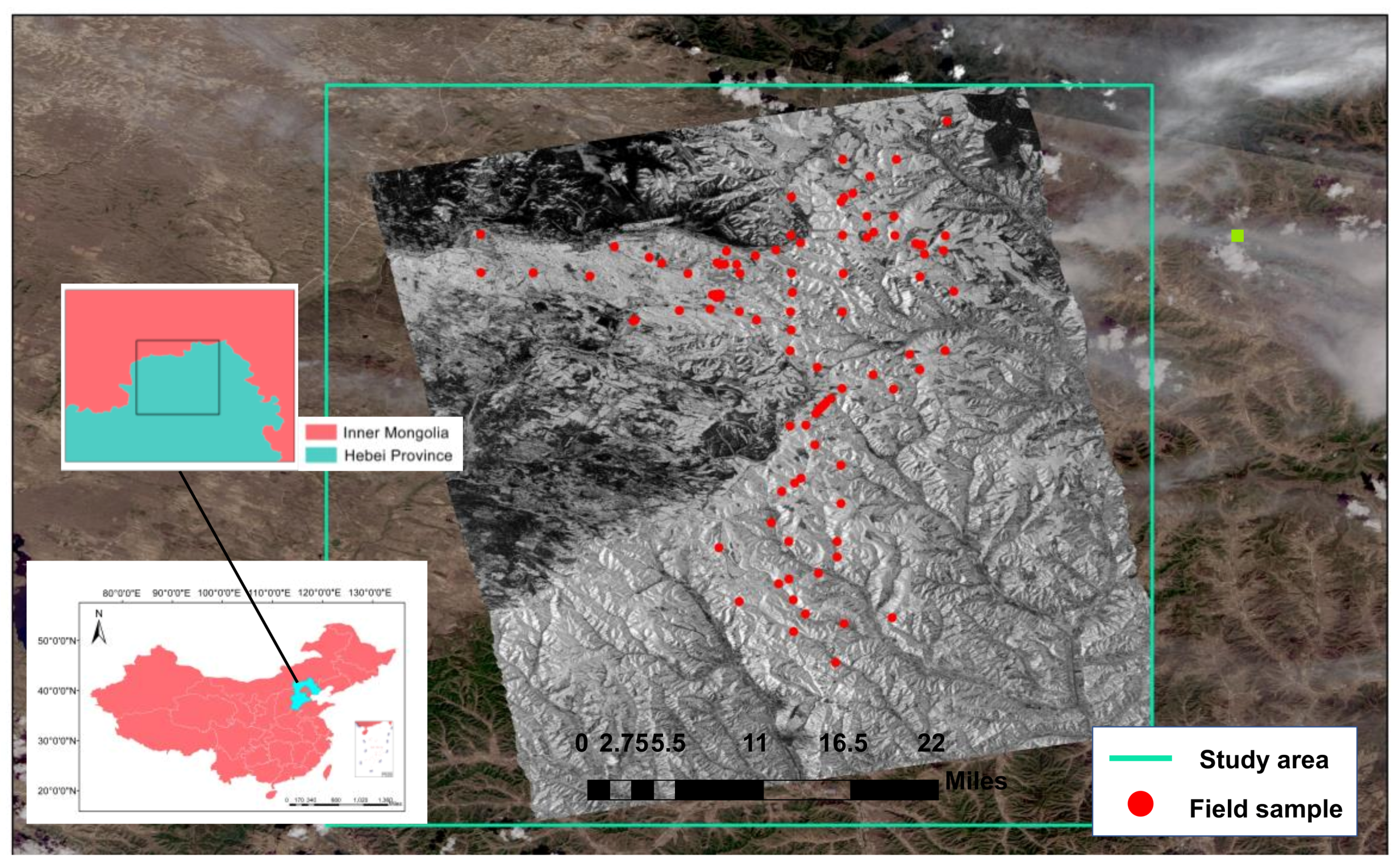
The study was conducted in Saihanba Forest, a typical temperate forest in northern China. The area is located in the transition zone from Yanshan Mountain to Inner Mongolia in Hebei Province (117°E, 42°N), and is the largest plantation forest in the world. The forest sites in the area are rugged and mountainous, with an average elevation of 1500 to 2067 m, making ground surveys difficult (Figure 1). The complex climatic conditions and the vulnerability of conventional imagery to weather conditions in the region make it necessary to conduct microwave observation studies in the region [51].
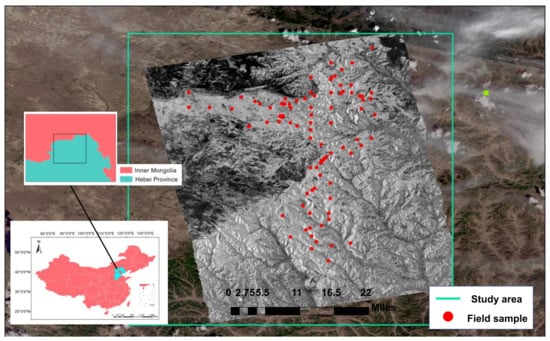
Figure 1.
Map of the study area. The area is located in the Saihanba Forest in Hebei Province, China. The red points represent the distribution of the measured samples. The image in the study area is an interferometric image under HV polarization of PolInSAR data.
The measured data from the plots was collected in the same study area as the PolInSAR data and randomly sampled within the study area. There are various types of forests in this area, and the main are temperate mixed conifer-broad forests. Larix principis-rupprechtii Mayr. and Betula platyphylla Suk. are the dominant species in the area. In addition, they include Picea asperata Mast., Pinus sylvestris var. mongolica Litv., and some broad-leaved species (Figure 2). During the field measurements, we conducted a careful field inspection before selecting the sample sites in order to make the samples better represent the overall condition of the forest area. Among the final collected samples, 28 plots were measured at fixed points on a kilometer grid, and the remaining 69 plots were randomly sampled, hoping to represent the real situation of the forest as much as possible. The proportion of stand types in the random sampling samples was ensured to be similar to the proportion of overall stand types in the forest area as far as possible, and the forest types in the sample sites are shown in Table 1. Furthermore, the forest management in Saihanba area is in good condition, with obvious differences in stand age and density. Due to tending and thinning, most of the forests gradually decrease in density as the forest age increases. In order to restore the true forest condition, at least 30% of the samples were guaranteed to be young (high-density stands) or old growth (low-density stands) during the sampling process.
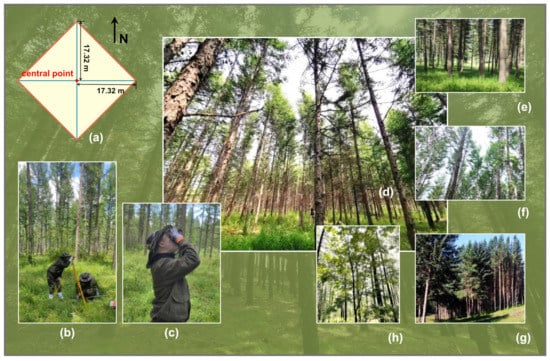
Figure 2.
Forest conditions in the study area and the sample plot survey. (a) The diamond-shaped sample with an area of 0.06 ha. Moreover, (b,c) show the determination of sample plots and measuring heights of trees using ultrasonic height gauge. Furthermore, (d–h) show forest conditions in the study area, where: (d) is the pure forest of Larix principis-rupprechtii Mayr.; (e) is the pure forest of Pinus sylvestris var. mongolica Litv.; (f) is the mixed forest of Larix principis-rupprechtii Mayr. and Betula platyphylla Suk.; (g) is the pure forest of Picea asperata Mast.; and (h) is the broadleaf mixed forest.

Table 1.
Forest types and the collected random sample sizes.
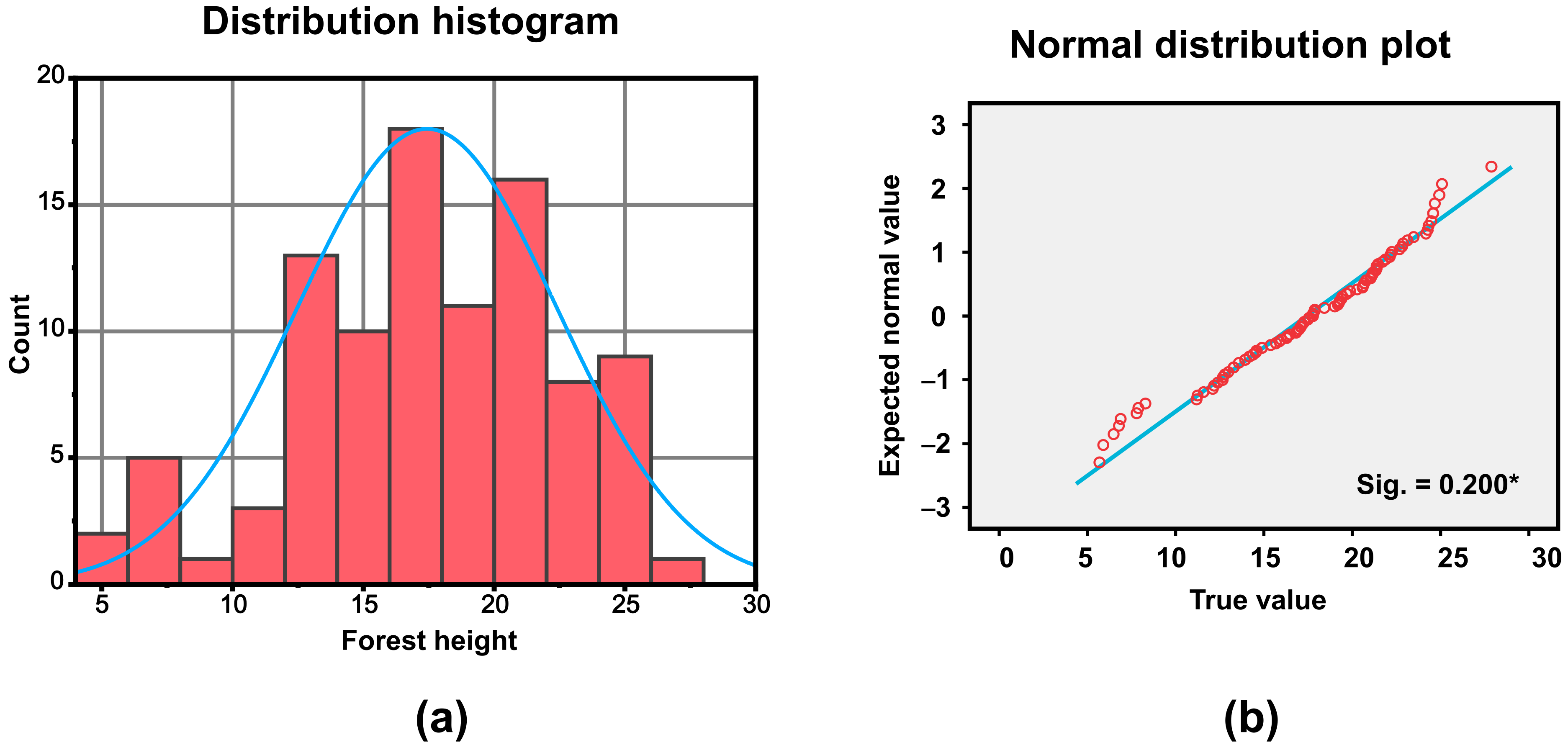
When collecting samples, we avoided the forest edge and large empty windows, and chose a relatively central position in the small forest class to ensure that the samples represent the real situation of the surrounding small forests as much as possible. After determining the center point, a distance of 17.32 m was measured along the four positive directions to determine the location of the four corner points, enclosing a diamond-shaped sample with an area of 0.06 ha (Figure 2a). The trees in the sample plot were inspected for each log, and the height of each log was measured with a Vertex IV ultrasonic height gauge. In this study, the forest height is defined as the average tree height of the sample plot. This assumption takes into account the value of average tree height in forest surveys on the one hand, and on the other hand provides support for the subsequent estimation of forest biomass. According to the field measurement results, the forest height was between 0 and 30 m, and the average height was 17.98 m. The Kolmogorov–Smirnov test was performed on the forest height sample data to test for normal distribution. The results proved that the sample data obeyed the normal distribution and has good representativeness (Figure 3).

Figure 3.
(a) Histogram of the distribution of the sample forest heights. The blue curve is the normal distribution curve. (b) Scatterplot of samples, normal distribution. The red points are the true distribution of the samples, and the blue line represents the standard normal distribution. The significance value Sig. was verified at the 0.05 level (*). And the samples showed a significant normal distribution after they were tested for normal distribution using the k–s method.
2.2. PolInSAR Data
The PolInSAR datasets from the study area were in five scenes of ALOS2 PALSAR repeat-pass fully polarized synthetic aperture radar data (Figure 4). The 1.1-level L-band SLC data were developed by Japan Aerospace Exploration Agency (JAXA). This data were used in this study because it is among the few commercial L-band segment satellite-based fully polarized SAR data that is publicly available worldwide. Additionally, the L-band is less sensitive to forest vertical heterogeneity and allows accurate inversion of forest height from empirical structure functions [52]. Therefore, it is important to study independent inversion of forest height from this data before the opening of the new low-band satellite-based SAR system.
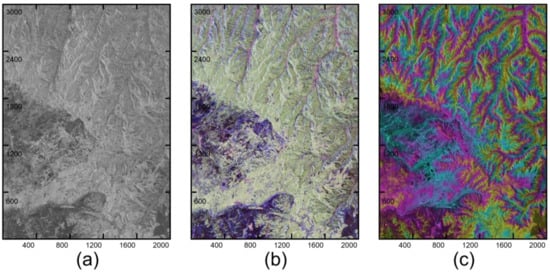
Figure 4.
(a) Grayscale image of the original L-band image under HV polarization; (b) PolInSAR image Pauli-based false color image; (c) interferometric DEM of the on-board data.
The datasets were collected over the study area from July to September 2020, representing the growing season of the forests in northern China. This was done within the same period the field observation data of the sample site was collected. The average zenith angle was 27.8°, the range pixel spacing was 5.66 m, the azimuthal pixel spacing was 2.86 m, the general observational area was 4944.62 km2, and the average height of the sensor from the Earth’s surface was 636.56 km. The spatial baseline length between different data ranged from 80.2 to 170.4 m. ranged from 0.012 to 0.021 rad/m, and the temporal baseline between two adjacent data were 14 days. The images acquired on different dates were combined as the interferometry primary and secondary data. Four groups of PolInSAR interferometric pairs with different temporal baselines and vertical wavenumbers were set up (Table 2). The inversion of each pair of interferometric data were done independently to compare and verify the results. The inversion process was repeated in each pair of interferometric data.

Table 2.
PolInSAR interferometric datasets.
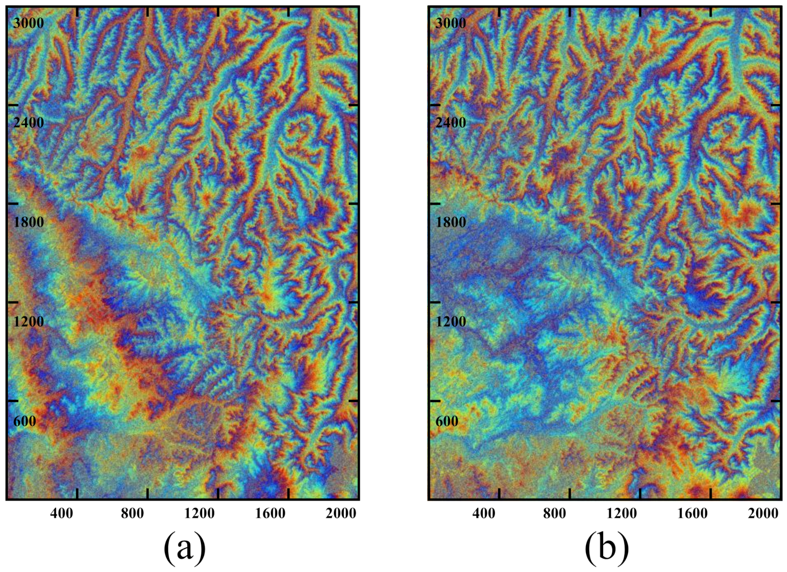
Each set of interferometric pairs was pre-processed to remove decorrelation geometrically using GAMMA software [53,54]. Meanwhile, ionosphere-induced phase drift and path delays are the main sources of error in ALOS2 repeat-pass spaceborne PolInSAR when performing interferometry [55,56]. In this study, the ionospheric effect was eliminated using the distance splitting spectroscopy method (Figure 5). Terrain correction was performed using 30 m resolution SRTM DEM data [57,58].

Figure 5.
Interferograms before (a) and after (b) reducing the phase drift and path delay caused by the ionosphere.
3. Theoretical Analysis of Forest Height Inversion
3.1. RVoG Model and Three-Stage Inversion Method
PolInSAR data combines both interferometry and polarization properties [59]. The complex interferometric coherence is obtained by combining the matrices and of the primary and secondary images at a particular polarization and can be expressed as follows:
where * represents the conjugate of the SAR image and represents the expected value [28,29]. The magnitude of the complex coherence () represents the coherence between two images (i.e., degree of similarity between two images), and its value ranges from 0 to 1.
Previous studies have shown that the complex coherence obtained by Equation (1) is still affected by several decorrelations even after eliminating system induced decorrelation [2,54]. The observed interferometric coherence can be modeled as a combination various contribution [54,55] and illustrated as follows:
Here, represents the decorrelation effect from thermal noise; is temporal decorrelation; and is volumetric decorrelation, which is widely used to forest height inversion. can be eliminated during image preprocessing. However, due to the constraints of a variety of factors, can introduce bias between and ; it not only affects the phase of , but also further reduces the overall coherence. For northern forests with lower forest heights, may sometimes mask the influence of , especially for repeat-pass spaceborne PolInSAR data with a temporal baseline of several days [28].
is included into the model to allow calculation of the forest height. The RVoG model combines the forest height with the scattering properties by treating the scattering as a volume scattering and ground scattering contributions through the assumption of the forest as a random homogeneous scatterer [28]. The model expresses the forest volume scattering complex coherence as follows:
where is the ground scattering contribution, m is the effective ground-to-volume amplitude ratio, and is the volume scattering complex coherence without the ground contribution. can be expressed by the mean extinction coefficient and the forest height as follows:
where is the vertical wavenumber.
is the radar incidence angle, is the incidence angle difference between the two images induced by the spatial baseline, λ is the wavelength, is perpendicular component of the spatial baseline, is the slant range, and is an integer constant that is equal to 2 for monostatic acquisition and 1 for bistatic acquisition.
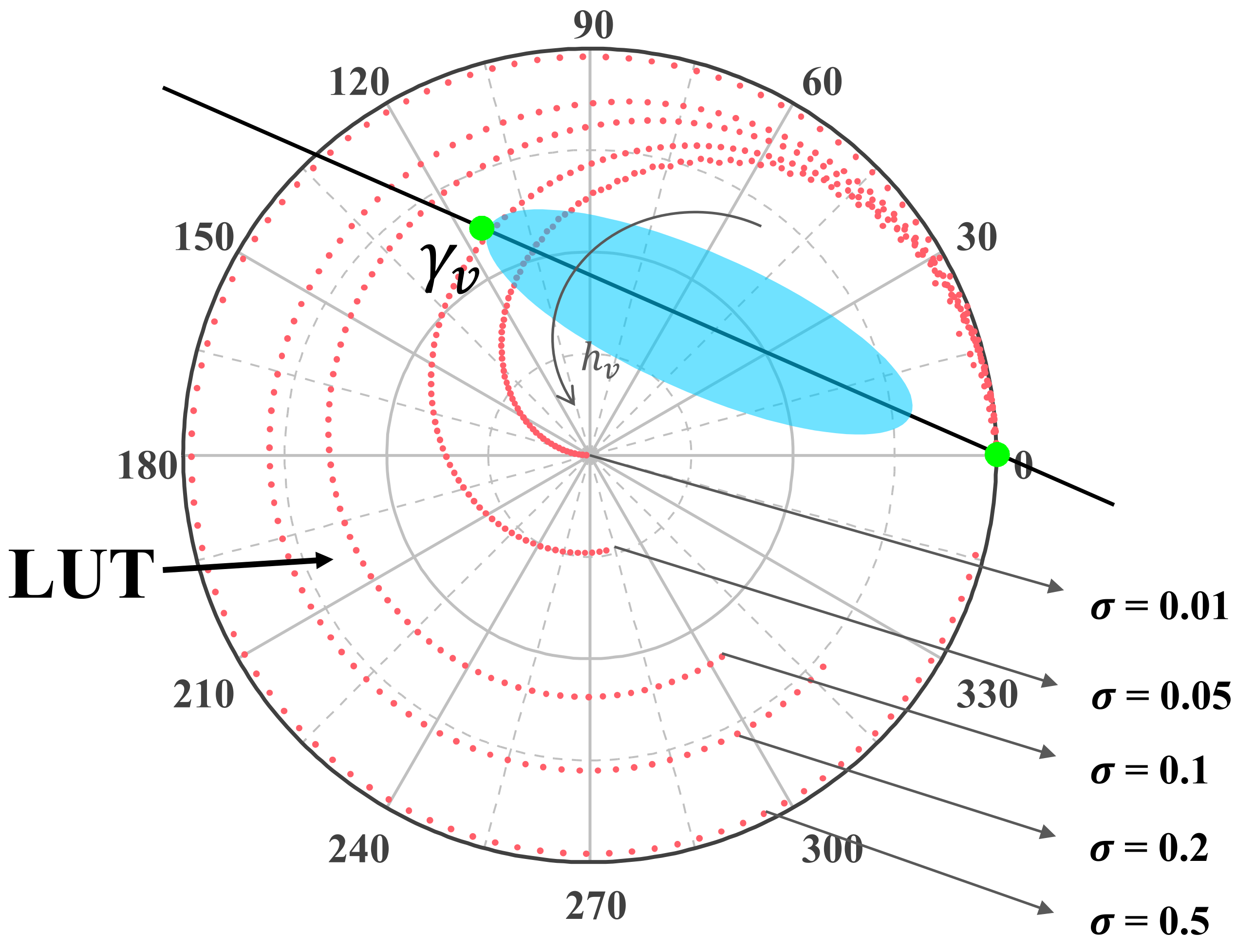
Since the ground scattering ratio is a parameter affected by polarization, Equation (3) can be observed as a straight line in the complex plane (Figure 6). The three-stage inversion method is applicable to PolInSAR developed from this geometric property [38]. The first stage of the inversion method uses different ground contributions contained in the different PolInSAR data polarizations, which fall at different positions in the complex plane (blue shade in Figure 6), and the coherence line of Equation (3) can be fitted. In the second stage, the two intersection points of the coherence line and the unit circle of the complex plane are determined as candidate points for the ground coherence point. The actual ground coherence point is determined through screening, and its influence is eliminated. In the third stage, a 2D lookup table of extinction coefficient and forest height (red points in Figure 6) can be established according to Equation (4). Generally, it is assumed that the complex coherence point under HV polarization is mainly volume-only scattering in InSAR, and the complex coherence in PolInSAR coherence optimization represents volume scattering, which allows forest height inversion, and determination of extinction coefficient value in the lookup table.
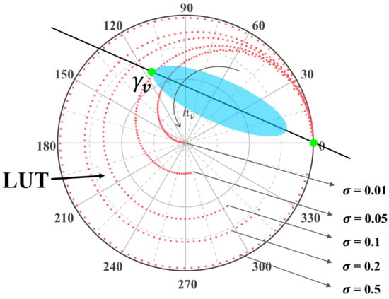
Figure 6.
Schematic diagram of the three-stage inversion method. The black straight line is the fitted coherence line, the blue shaded area is the coherence region composed of different polarized coherence points, the green points indicate volume-only scattering and ground coherence points, and the red points indicate the 2D lookup table calculated by the RVoG model, in which the average extinction coefficient values of the points in each curve are the same, but gradually moves away from the phase origin as the forest height increases. The different curves represent different average extinction coefficients, and the closer they are to the circumference, the larger the value of extinction coefficient. Moreover, in the figure is 45°, ranges from 0 to 50 m, and the interval between two adjacent points is 0.5 m.
3.2. Temporal Decorrelation
The temporal decorrelation of interferometric image often causes obvious errors to the inversion results, regardless of whether RVoG model or other interferometric inversion models are used. Temporal decorrelation reduces the coherence and causes a phase shift of the interferometric data so that the forest height inversion model is greatly affected. The error sources of temporal decorrelation have a complex structure [42] and are influenced by combination of factors that are difficult to quantify. As a result, temporal decorrelation is difficult to remove when pre-processing image data.
In general, the degree of temporal decorrelation is described by the temporal baseline, which is the time interval between primary and secondary image observations. Data with larger temporal baselines undoubtedly face greater temporal decorrelation. The temporal baseline of repeat-pass spaceborne SAR data for the same observation area tends to be more significant compared to airborne PolInSAR data. This study’s temporal baseline of ALOS2 repeat-pass spaceborne SAR varies from a few days to tens of days. Therefore, there is a larger temporal decorrelation contribution in the repeat-pass spaceborne SAR interferometric data. In addition, the sensitivity of different images to the same temporal decorrelation of the interference varies and PolInSAR data with smaller has a more pronounced response to temporal decorrelation. For the InSAR, is defined by the angular difference between the primary and secondary sensors (Equation (7)) and is a factor that indicates the sensitivity of the interferometric phase to changes in terrain (height) [49]. For the PolInSAR inversion forest height model, the smaller makes the forest height more sensitive to changes in the coherence and phase of the interferometric data during inversion [49]. Therefore, when using interferometric images with small to retrieve forest height, there may be huge errors in the inversion results even if there is a weak temporal decorrelation factor [50]. The situation is reflected in the absence of intersection between the observed complex coherence in the unit circle and the LUT when using the three-stage inversion method for height inversion [60]. Meanwhile, the of repeat-pass spaceborne PolInSAR data tend to be lower, making the inversion results (which already contain a large temporal decorrelation factor) less accurate. Therefore, it is necessary to adopt an effective correction for temporal decorrelation inversion model when retrieving forest height from repeat-pass spaceborne PolInSAR data.
There are several improved models for temporal decorrelation including the RVoG+VTD model [60], the RMoG model [35,43], and the semi-empirical iterative model for dielectric constant and random motion modeling using Gauss-Newton iterative optimization model [42,48].
The RVoG+VTD model demonstrates that, temporal decorrelation shifts the volume-only coherence points in the complex plane unit circle during the inversion using the three-stage method. As such, there is no intersection between the height-extinction LUT and the volume-only coherence point. Therefore, correction terms for the shifted volume-only coherence points are achieved by fixing the extinction coefficient and using the SINC function. Meanwhile, RMoG model is different from the RVoG+VTD model since the effect of temporal decorrelation on volumetric decorrelation is not considered to be a multiplicative relationship. This model quantifies the cause of temporal decorrelation as a stochastic motion parameter that varies with the forest canopy. This was the first method to attempt to model the direct extraction of forest height from the mixed effect of temporal decorrelation and volumetric decorrelation. Additionally, a ten-dimensional parametric model was developed from the observations under different polarization channels. Another study decomposed temporal decorrelation into the temporal effects of dielectric constant variation and random motion, used coherence to build an empirical model, and extracted the parameters using the Gauss-Newton iterative method [42,48]. The forest height model can use the repeat-pass spaceborne InSAR data in L-band with large temporal baseline.
4. Improved Inversion Model
In this study, a new inversion method has been proposed to enable forest height inversion by empirical iteration. Corrections were performed to degrade coherence and phase shift caused by error sources such as temporal decorrelation. In addition, the inversion accuracy of the improved model was simulated, and its geometric process was analyzed theoretically.
4.1. Theoretical Background
The interferometric phase obtained from the interferometry can be used to calculate the topographic height of the ground surface.
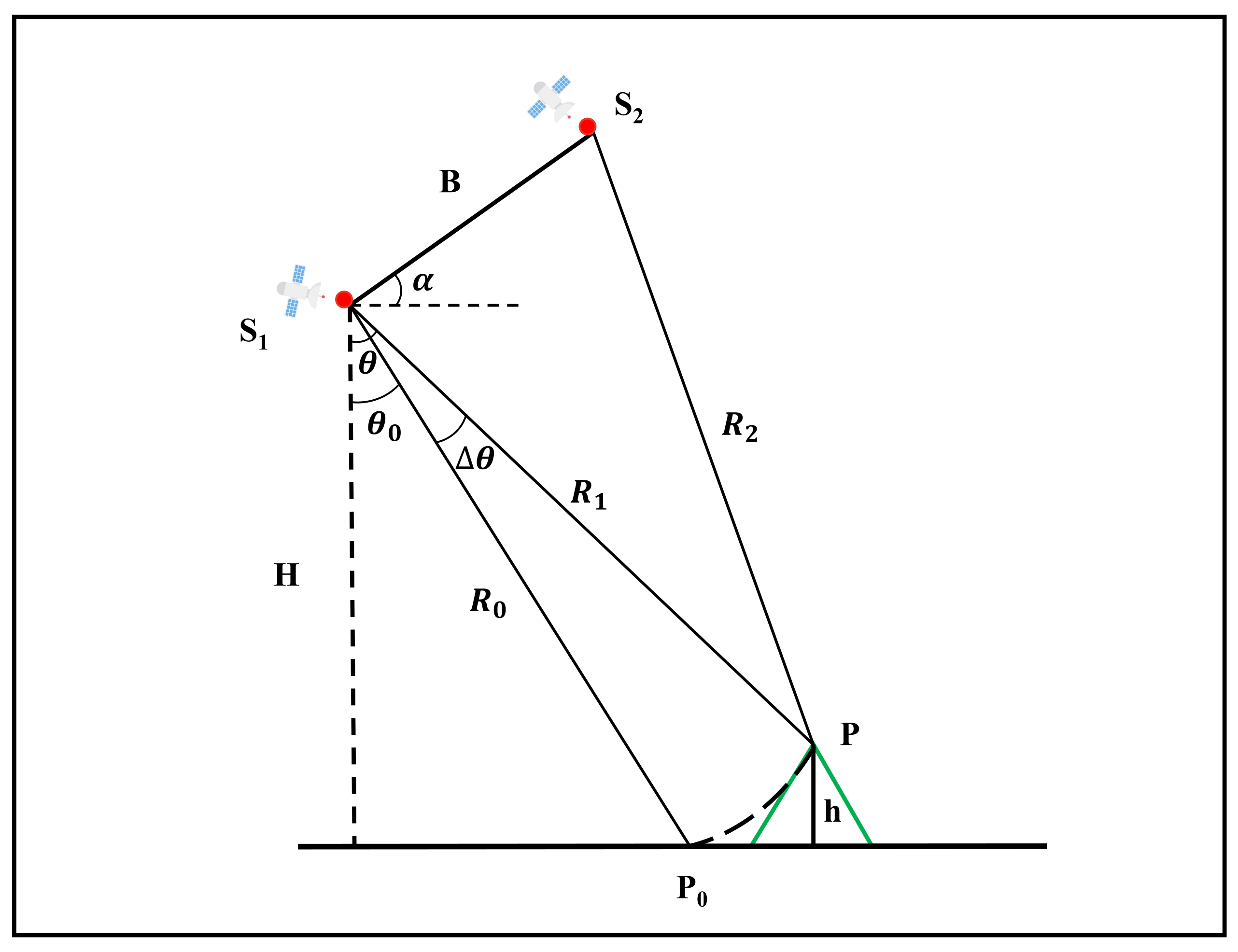
In repeat-pass interferometry, the same sensor makes two recordings of the same ground target at a certain time interval to form an interferometric data pair (Figure 7). The first recording is referred to as the primary image (marked as ), and the second recording is referred to as the secondary image (marked as ).

Figure 7.
Schematic illustration of Interferometric geometry.
The primary and secondary images are conjugated and multiplied to obtain the interferometric phase values.
When phase ambiguity is not considered, the interferometric phase can be expressed as follows:
where is the difference between and radar wave propagation distances.
The interfering phase consists of the following five main components:
- Flat Earth phase due to reference ellipsoid.
- Topographic phase due to terrain undulation.
- The deformation phase caused by the deformation of the ground surface during the two imaging sessions.
- The phase difference caused by atmospheric disturbances.
- The phase difference due to noise.
In this study, the ground surface was considered undeformed. The atmospheric and noise disturbances were ignored.
After eliminating the above interference factors, only the flat earth phase and the topographic phase remained in the interferometric phase. The geometric principle of interferometry is explained using a previous example where the topographic height h was measured at the surface target point P in Figure 7 [16]. Point P in the figure is the target point of interferometry. is the point on the reference ellipsoid, and it allows equal distance from to P and .
When the sensor is far enough from the ground target, the component of the spatial baseline (between and ) that is parallel to the line (between and P) can be approximately equal to (). The topographic phase at point P is expressed as follows:
B is the spatial baseline between and , is the angle between the line connecting to the ground target point P and the vertical direction, and is the angle between the baseline B and the horizontal direction. The flat earth phase at point is as follows:
is the component of the spatial baseline B that is parallel to the line between and , is the angle between lines and and the vertical direction, and is the flat earth phase corresponding to the point P. Meanwhile, the phase difference between P and can be expressed as follows:
The angle between and is very small, due to the long distance between the sensor and the ground target. Thus, Equation (11) can be simplified as follows:
is the component of the spatial baseline B, which is perpendicular to . In the geometric relationship illustrated in Figure 7, the value of the height of point P is computed as shown below:
h is the height of the ground target point P from the horizontal plane, H is the height of from the horizontal plane, is denoted as the radar wave propagation distance of , and is the difference between and . Therefore, the topographic phase and height can be expressed as shown in the equation below:
The first term on the right side of the equation is the terrain phase given the terrain height, while the second term is the flatland phase considering the zero change in elevation. After removing the flat earth phase, we obtain a linear relationship between height and terrain phase, and it is linked by .
The above equation showed terrain height measurement by interferometric phase. However, there is a significant difference in measurements when using PolInSAR to measure forest height. Meanwhile, the interferometric phase between the top point of the canopy and the underlying surface point should be included in the calculation of forest height. However, the observed phase at the top of the canopy had two-phase contributions in addition to the five components mentioned in Equation (8). The first contribution is the shift of the phase center caused by the penetration of low-frequency SAR into the forest canopy [53]. The second contribution is the phase shift caused by random movement of the canopy during the imaging of the primary and secondary images [43]. Both of these contributions interfere with the forest height measurement and should be eliminated during the inversion process.
The geometry of the forest height measurement by interferometric phase is illustrated in Figure 8. is the phase center at the top of the canopy. However, the phase shift caused by the random motion of the canopy causes the phase center of the canopy to shift to when being observed. The shift in phase center that is caused by low-frequency SAR penetration makes it possible for the observed phase to lie anywhere between and . is the corresponding point on the reference ellipsoid. The interferometric phase and the height from the horizontal plane at are then described as follows:
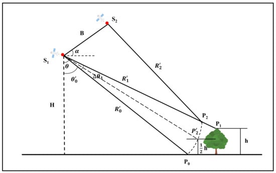
Figure 8.
Schematic diagram showing the phase shift of the observed target. is the component of the observed phase on the line of sight affected by random motion, is the height reduction at the center of the phase caused by microwave penetration, and is the true phase point.
The relationship between interferometric phase and height at point is as follows:
where is the difference between and . is the height difference between and , and the offset of the measured height of the canopy. The second term on the right-hand side of the equation is the flat-earth phase of . The above two interference factors influence the height deviation, so it is necessary to quantify the height error of the two effects. Previous studies have described random motion as Gaussian function that varies with height and uniformly when in the vertical direction [35,43]. There was neither deformation on the surface nor phase difference caused by random motion on the surface. When only the offsets produced by the random motion on the canopy are taken into account, the height offset can be considered as a linear function of the canopy height and can be expressed as follows:
where denotes the standard deviation of the motion at a certain reference height , and represents the variation of this offset from the height.
Previous studies have focused on the modeling of random motion and understanding the relationship between interferometric coherence and random motion. However, the effect phase shift errors on the height inversion results may be more pronounced. Therefore, this study attempts to correct this error and improve accuracy in the height inversion results.
Meanwhile, the phase bias caused by low-frequency SAR penetration makes the observed phase lie between the top of the canopy and a half of the height [53]. Therefore, the height deviation obtained by coupling the two factors can be simplified as a linear function that changes with the vertical target height:
where is the distance between the scattering center and the underlying surface after the canopy phase shift . The height error was brought into the canopy phase without the flat-earth phase in order to obtain the relationship between the observed canopy phase and the true canopy height. The equation is as follows:
where is the correction term for temporal decorrelation due to random motion, and is the corrected phase for the phase center shift. Noteworthy, , .
Temporal decorrelation not only causes phase shift but also leads to a reduction of factors affecting interferometric coherence, such as dielectric constant with temporal baseline. This also has a more pronounced effect on the PolInSAR inversion of forest height and, therefore, measures are needed to reduce this interference. In order to address the apparent temporal decorrelation of coherence amplitude, phase interference, and canopy phase center shift suffered during the repeat-pass spaceborne PolInSAR inversion, this study proposes a new inversion method to achieve the inversion of forest height by empirical iteration. First, to address the interference of temporal decorrelation on the interferometric coherence and correct the overall coherence, this study introduces a correction term based on the RVoG model (Equation (4)):
With respect to the offset phase caused by the random motion and microwave penetration factors in the temporal coherence, the offset phase value of the height modeling in Equation (21) is introduced into Equation (22) as follows:
where .
In previous studies, the physical model construction method [35,42] decomposed the temporal decorrelation into factors such as dielectric constant and random motion, and then modeled together with volume decorrelation to extract forest height. These models are undoubtedly advanced and effective, but often require complex iterative processes and have many model parameters, which increases the uncertainty of the inversion. This study attempts to use an empirical model to achieve fast and efficient inversion, and achieve results that are similar to previous temporal–decoherent models. Therefore, the model is built based on the three-stage inversion method, and the geometric properties of the model are used to improve efficiency of the inversion. The error factors encountered during the inversion are integrated into Equation (23) as a correction term on the phase, and a complex correction term . They are both brought into the iterative process to ensure that complete error sources are considered in the model.
The model is performed under the assumption that is in line with , but this does not affect the validity of the model. This study focuses on the height difference in the vertical direction between and , and does not require obtaining of the specific true phase point. Therefore, even if the two are not on the same line, the inversion results in another point with the same height on the line. Moreover, since this is an empirical model, the real data are used as prior information. Therefore, forest height can be calculated based on this assumption.
4.2. Iterative Process of the Improved Model
The iterative process of the improved model follows the flow of the three-stage inversion method. First, the polarized interferometric information needs to be extracted from the pre-processed PolInSAR data. Each set of polarized interferometric data pairs contains the original complex data under full polarization, and the Pauli basis scattering vector for each set of images is as follows:
where represents the scattering matrix elements collected twice at different polarizations, represents horizontal polarization, and represents vertical polarization. represents the transpose of the matrix. With the Pauli basis vector, we can obtain the T coherence matrix and the matrix as follows.
T coherence matrix:
The matrix:
where denotes the mathematical expectation, and is the conjugate transpose.
With the T matrix and matrix, we can calculate the coherence and the phase of the primary and secondary images with different polarization and coherence optimization. This study employs the common and easily extracted complex coherence values, including three basic polarization types HH, HV, VV, four linear combinations of different polarizations (HH+VV, HH-VV, HHVV, HV+VH), three circular polarizations (LL, LR, RR), three Opt coherence optimizations (Opt1, Opt2, Opt3), and two PD coherence optimizations (PD High, PD Low). Due to the specific polarization correlation of the ground scattering contribution, the 15 complex coherences have different ground scattering ratio coherence.
The improved model extracted the volume-only scattering complex coherence method in general agreement with the three-stage inversion method. During the inversion, 15 types of complex coherences were projected into the unit circle of the complex plane. The least-squares method was used to fit the phase trunk using the different scattering ratios of the earth’s surface under different polarizations. The two intersections of the fitted coherence line and the unit circle of the complex plane allowed determination of the candidate points for ground coherence. The external DEM phase in this image was compared with the candidate points and filter to identify the true ground coherence points and remove their influence. After the removal of terrain phase, the coherent region of each pixel was obtained, and the volume-only complex coherent points in each pixel were screened by comparing the distance between the optimized complex coherent points and the ground coherent points.
Once the volume-only scattering complex coherence is scattered, a 2D look-up table of forest height-extinction coefficients is a requirement in the flow of the three-stage inversion method. The forest height and extinction coefficient values are obtained according to the intersection of the LUT and the volume-only complex coherence.
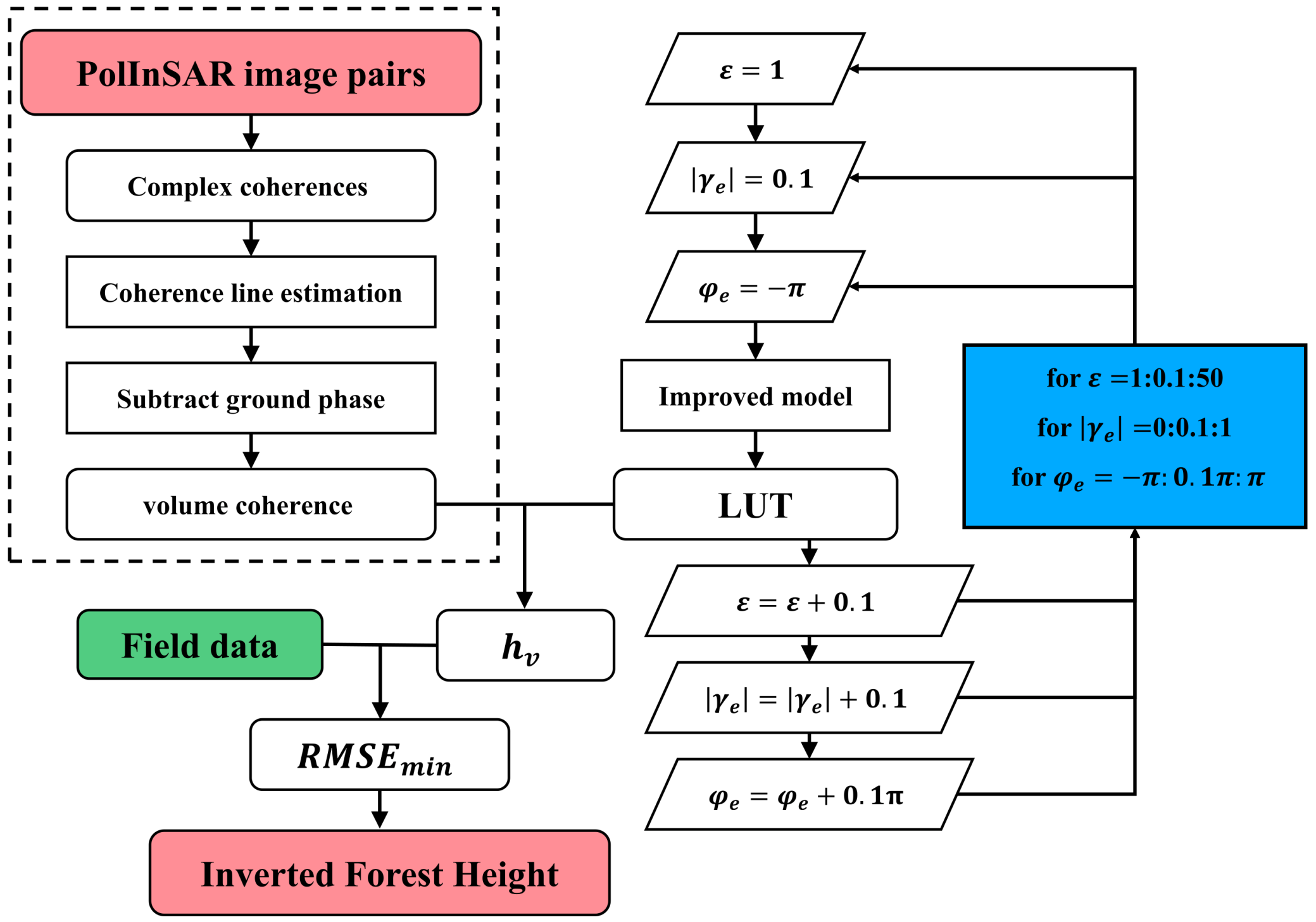
In this study, the process of improving the model is illustrated in Figure 9. After introducing and into the RVoG model (through Equation (23)) as unknown parameters, a new set of LUTs was generated when the amplitude and the phase of and had different values. A triple iteration of the LUT was then performed after setting the range for the parameters. The intersection of each set of LUT with the volume-only decorrelation performed the forest height inversion under the set of parameters. Meanwhile, iteration added unknown parameters to the model. Therefore, the improved model needs the control condition of iteration, which is the true height measured on the ground. In this study, 25% of the ground-measured forest heights was randomly selected as the priori data for the iterations. The best parameter values in the iteration range and the corresponding inversion results were obtained by calculating and comparing the RMSE of each set of inversion heights with the ground data.
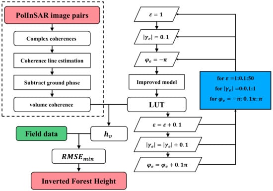
Figure 9.
The inversion flow chart.
The improved model performs height inversion for all regions in the image, which was consistent with the original inversion method. The iterative parameters and in the model are calculated at the image level, and only one parameter result is iterated for the same group of interferometric pairs. Therefore, the real ground measurement data used in the inversion need at least one true value that is a true reflection of the forest height in the image. This is particularly important in controlling the inversion error in order to understand forest height inversion from the image and create a balance in the model.
4.3. Theoretical Analysis of the Improved Model
In this study, the improved model is an empirical model. Besides the control of ground data, selecting the initial range of empirical parameters also has an important impact on the results. To discuss the feasibility of the improved inversion model, and establish whether the model satisfies the inversion conditions, this study theoretically tested the improved model using simulated data.
Previous reports have shown that the magnitude of the vertical wavenumber determines the sensitivity of the inversion results to temporal decorrelation interference [49,50]. The simulated data in the present study was therefore created to invert the study areas with different mean tree heights () using PolInSAR with different . When a certain degree of temporal decorrelation interference is present, the use of improved model to compute the relative height error () can reduce the relative error to less than 15%.
The distribution of error in the inversion results is shown in Figure 10. As the control variable, the interference size of to the simulated data are fixed at . The average extinction coefficient and the observation Angle are also fixed. For each given , the corresponding volume-only complex coherence for different can be calculated using Equation (4). When is multiplied with the set , the relative errors of the improved model inversion results under different can be simulated in the actual inversion process. Based on Figure 10, it can be noted that when no improvement is made to the model (when is 1), the inversion error gradually increases with the decrease of . When = 30 m, value larger than 0.05 is needed to determine forest height within 15% of the inversion error. Moreover, when is smaller, the inversion can only be accurate with larger . As increases, there exists one or more intervals of value for the compensated three-stage improvement method to accurately invert forest height within 15%, regardless of the size of taken from the interferometric data. Besides, when increases and reaches the next interval suitable for inversion, the range of this interval will be larger than that of the previous interval. This moderates the inversion error change, and makes the model more adaptable to the forest height change in the observed area. However, when the value selected for inversion is too large, the inversion error will be very unstable. The error of the inversion result changes rapidly and loses regularity when the change of and are not apparent. Inversion in this range will undoubtedly reduce the accuracy of inversion. Therefore, it should also try to avoid selecting too large ε to avoid fluctuations in the accuracy during the inversion.

Figure 10.
Distribution of relative inversion error of forest height with variation of and ε under different . The relative error is defined by , is set to , is 0.2, ranges from 0 to 0.1, and ranges from 1 to 50.
Figure 11 shows the simulated errors of the inversion of the improved model for different coherent amplitude and . Under the same conditions in the inversion process, the variation of coherence amplitude has little influence on the value of in the same inversion (Figure 11a). In the phase, change of will affect the value of . The larger the , the larger the value of when taken at the same (Figure 11b). Therefore, it can be proved that the influence of decorrelation on the inversion accuracy is mainly due to the phase change caused by . Based on our results, small was found to be more sensitive to phase change and highly likely to cause significant errors, which was consistent with previous research results [49,50]. In addition, the decrease in coherence amplitude caused by temporal decorrelation had an effect on the inversion results, and should not be ignored.
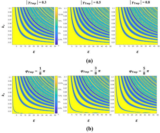
Figure 11.
Distribution of relative forest height inversion errors with and for different temporal decorrelation effects. is set to 20 m, is 0.2, ranges from 0 to 0.1, and ranges from 1 to 50. (a) Plots of forest height errors for different coherence amplitudes, with phase set to 0. (b) Plots of forest height errors for different phases, with amplitude set to 0.5.
The most significant difference between the improved model in this study and previous models is that it is an improvement on the three-stage inversion method, which is based on the geometric properties of the model. Therefore, there is need to analyze the geometric significance of the parameters expressed in the inversion process in order to understand each parameter’s intrinsic logic in improving the accuracy of the inversion.
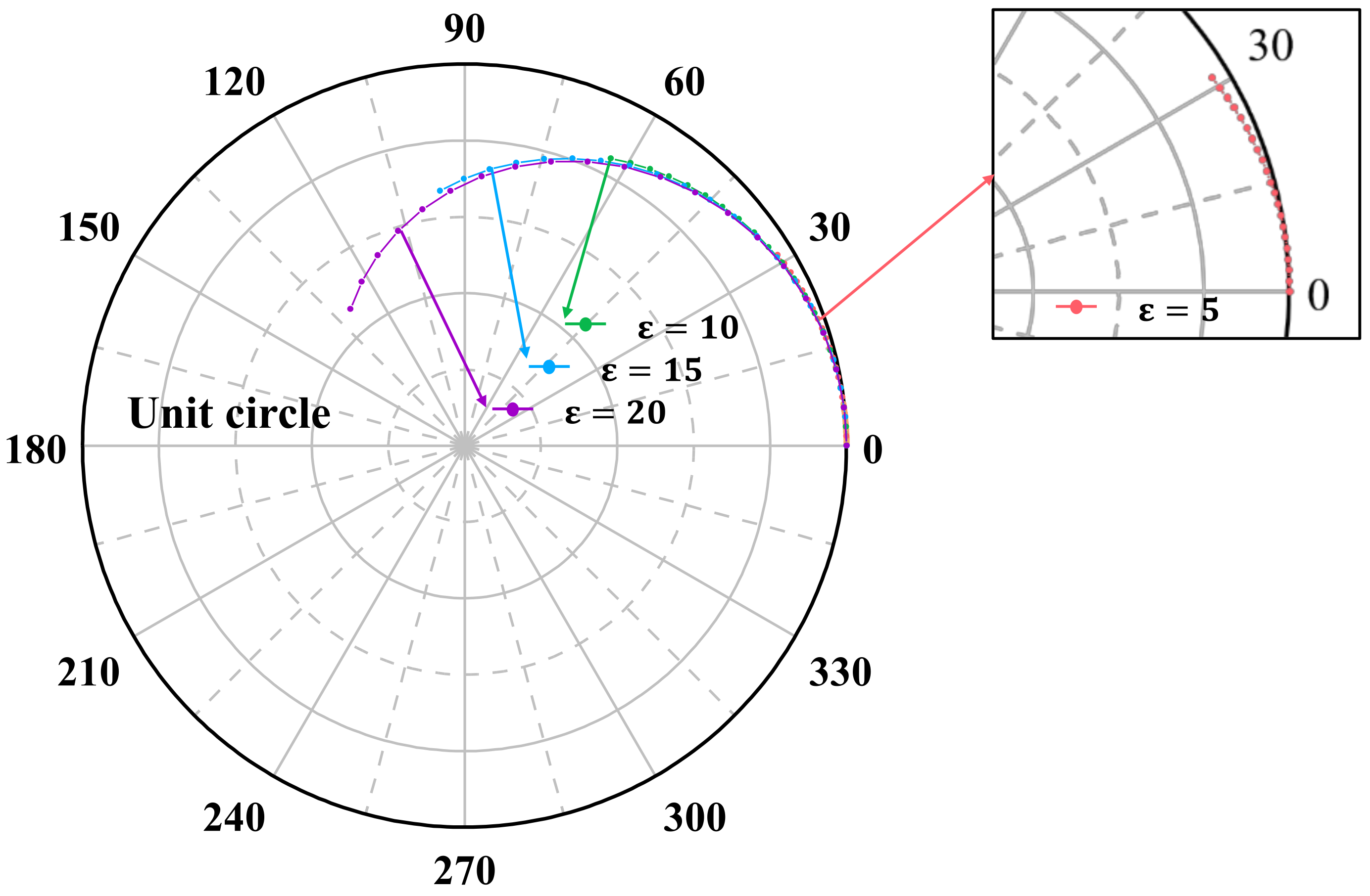
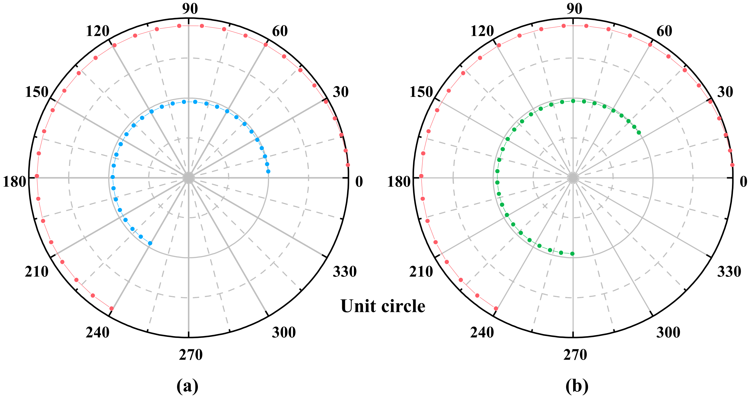
The correction term ε on the phase was corrected for the phase shift with height, and it ranged between 1 and 50 as shown in Figure 10. When the phase is corrected by using , the sensitivity of to complex coherence changes in the complex plane unit circle is reduced, the phase value at the maximum height is increased, and the coherence amplitude is decreased (Figure 12). In this case, it confirmed that there is an intersection point between the height-extinction coefficient curve and the volume-only coherence point. This method achieved accurate inversion results. Meanwhile, the magnitude of the complex correction term is the correction for the reduction of coherence due to decorrelation (), while the phase is the correction for the change of scattering center (). In the complex plane unit circle, moves the curve in the lookup table closer to the center of the circle (Figure 13a), and causes changes in the starting phase of the lookup table curve (Figure 13b). Therefore, the constant change of parameters during the iteration process generates new inversion results.
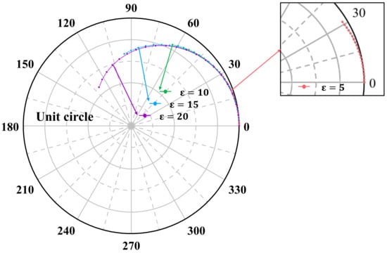
Figure 12.
Schematic diagram of inversion with ε under the improved model. In this figure, is 0.2, ranges from 0 to 30 m, the interval between two adjacent points of the same curve is 1 m, and is set to 0.01. differs between different curves, and the interval between two adjacent points gradually increases as increases. When reaches 30 m, the phase gradually moves away from the origin. During the inversion process, an increase in will expand the phase when reaches the upper limit of the phase of LUT. Besides, the sensitivity of gradually reduces changes in , making it more suitable for forest height inversion.
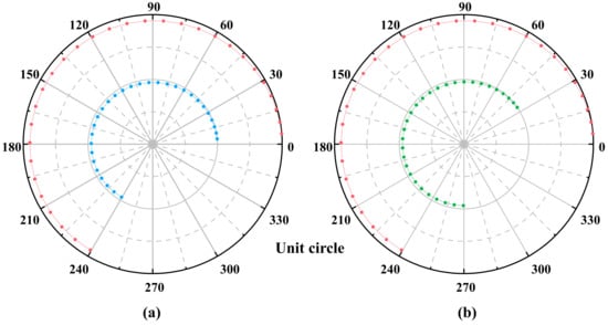
Figure 13.
The complex correction term changes the position of the LUT in the complex plane unit circle. (a) In order for to reduce the coherence amplitude of the LUT points, the curve composed of red points is the LUT calculated by the original RVoG model, and the curve composed of blue points is the LUT after correction, and its more suitable for the inversion of low coherence cases. (b) Shows the LUT after is introduced on the basis of (a), and the curve composed of green points is the LUT after correction, which is more suitable for inversion of data with obvious phase center shift. is 0.2, is 0.01, is 15, and the forest height range is 0–30 m with 1 m interval between two points.
5. Results
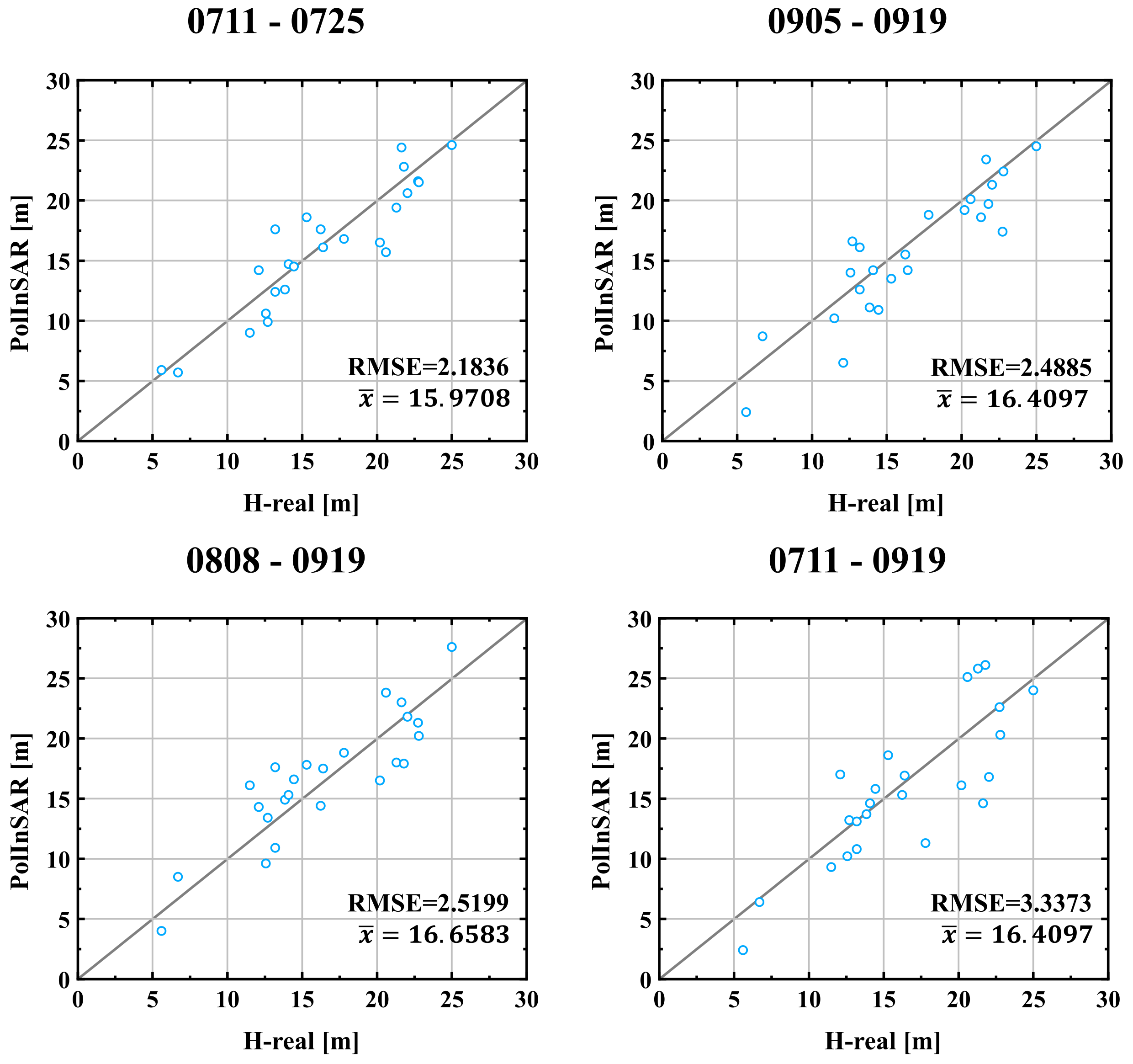
A total of 25% of the ground measured height was randomly selected as the prior data to control the iterative process. The inversion process follows the inversion procedure in Section 4.2. After quantifying the inversion error (Figure 10 and Figure 11), the initial range limit of was set to 1–50, the initial range limit of was set to 0–1, and the phase was set to . Figure 14 shows scatter plots of height results of the iterations using the improved model, with prior true data. Table 3 shows the iterative results and the inversion accuracy.
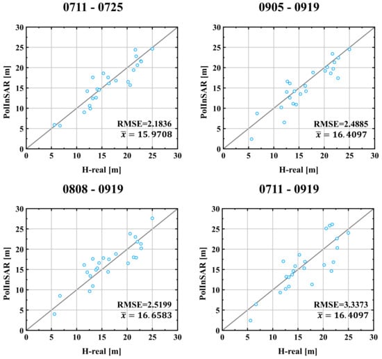
Figure 14.
Scatter plots of the height inversions based on the improved model and prior true height. RMSE and are the root mean square error and the mean value of the inversion results, respectively.

Table 3.
Iteration parameters and inversion accuracy.
It can be noted that the inversion results of the improved model were all within 15% RMSE compared with the true values, and there was a good fit. The iteration parameter ε ranged from 20 to 40, indicating that the random motion of the canopy produces a more significant interference with the phase error of the repeat-pass spaceborne PolInSAR data. Moreover, the decorrelation correction term of the parameter became larger as the temporal baseline increased. This indicates that the improved model has a better correction for the interference of temporal decorrelation. However, the magnitude of does not increase with the temporal baseline across the data but decreases with increasing . This also shows that the smaller the , the greater the sensitivity of the data to temporal decorrelation, leading to a decrease in inversion accuracy.
The inversion accuracy was found to be suitable for height inversion. However, all the relative standard deviations (RSDs) of the models were around 30% (Table 3), indicating that the inverse performance of the models still exhibits some volatility and randomness on a few samples. This phenomenon may be because the effects arising from temporal decorrelation were not completely eliminated by semi-empirical iterations. The calibration of temporal coherence could improve the deviation of coherence, but cannot solve the increase of phase line fitting variance caused by low coherence [49]. In addition, since the conditions of forest height and coherence between different elements in the same image are not the same, the size of the correction term is subject to various constraints. As such, the use of the same correction term may inevitably lead to inconsistent parameter effects of different pixel values. Nevertheless, the errors in the inversion results are still within reasonable limits and do not affect the forest height distribution or hinder further studies.
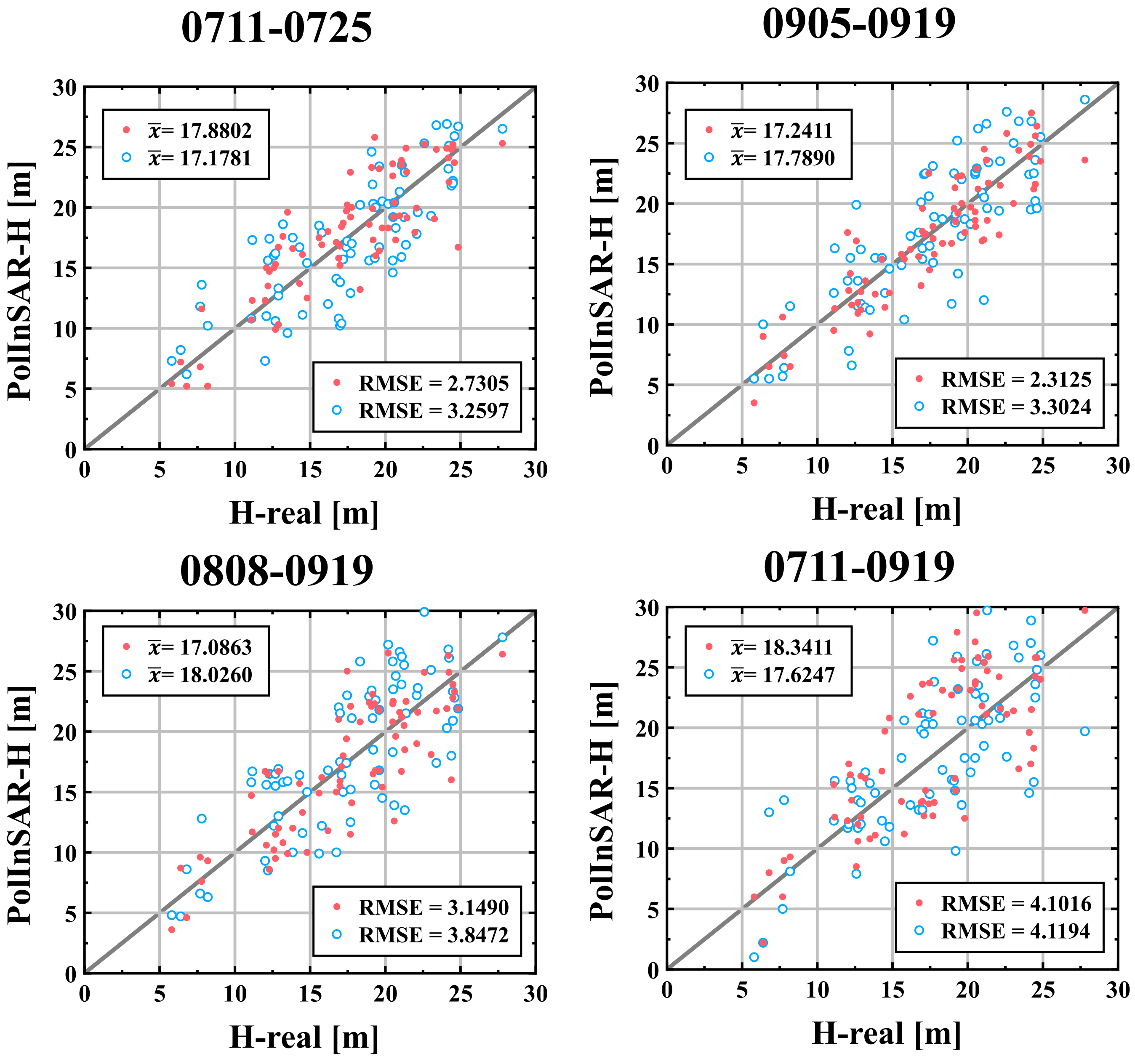
To test the robustness of the improved model, the iterative model was validated using an additional 75% of the ground truth data. Performance of the model was further evaluated by introducing the nonlinear least squares inverse model based on repeat-pass spaceborne InSAR [42] for comparison. In this model, the coupling coherence of volume decorrelation and temporal decorrelation is taken as the image observation, and the random motion of forest and the change of dielectric constant are taken into account under a certain temporal baseline. The model can be expressed as follows:
where is a non-negative real value less than or equal to 1 and represents the random motion level of the volume scatterers. Consistent with the original study, HV polarization was used in this study as the polarization to represent the volume scatterer. The same modeling data as the improved model in this study were used for training, and the model parameters were obtained by nonlinear least squares iteration. The scatter plots of the height inversions using models and the validation data are shown in Figure 15. The validation accuracy of the four data sets is also shown in Table 4.
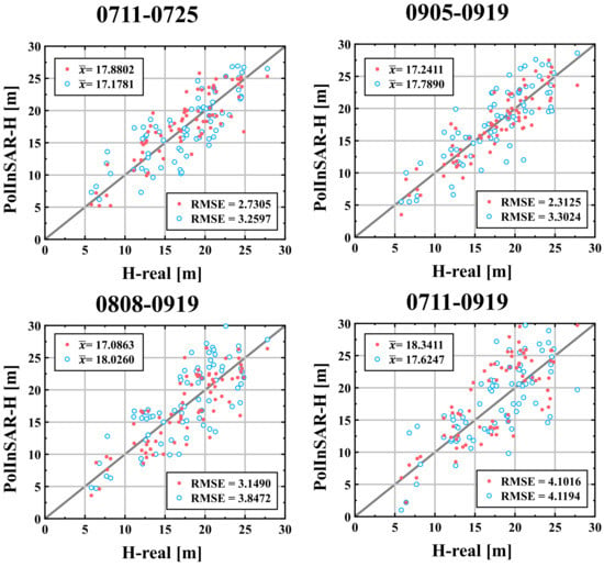
Figure 15.
Scatter plots of the height inversions based on the improved model and the validation data. The red points are the inversion heights of the improved models proposed in this study. The blue points are the nonlinear least squares model inversion heights. RMSE and are the root mean square error and the mean value of the inversion results, respectively.

Table 4.
The validation accuracy of the four data sets.
Based on Figure 15, it can be noted that the inversion accuracy of the improved model is relatively close for different interferometric pairs. Therefore, the model can still perform forest height inversion within 15% accuracy even when the temporal baseline is different from . This indicates that the inversion of the improved model is more robust and can be applied to repeat-pass spaceborne PolInSAR data with larger temporal baselines and smaller . In contrast, the nonlinear least squares model had lower inversion accuracy and a larger randomness due to the lack of correction phase. The accuracy of the model decreased more obviously when the data with large temporal baseline was inversed. Moreover, the lack of polarization information may be another reason for the decrease in accuracy.
6. Discussion
By improving the model inversion of forest height, the significant errors caused by repeat-pass spaceborne PolInSAR temporal decorrelation are reduced, increasing the scope of application of this data in forest height inversion. Based on the results of the improved model in Section 4 under different interferometric data, the following conclusions can be drawn:
- The correction of temporal decorrelation can improve the robustness and accuracy of the inversion and meet the needs of remote sensing for forest height inversion.
- A more accurate forest height inversion of common SAR data can be performed using the improved model, but there may still be a small degree of error in the inversion results.
- Data with large temporal baselines should be carefully selected when using models for height inversion.
6.1. Inversion Performance of the Model
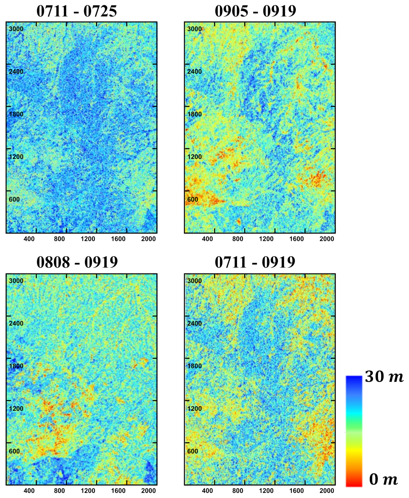
Temporal decorrelation causes abrupt changes in the interferometric phase on the one hand and decreases in coherence on the other. In Figure 16, the coherence of the larger temporal baseline is lower than that of the smaller temporal baseline, which also proves that for repeat-pass spaceborne PolInSAR data, temporal decorrelation is the main source of inversion errors [61]. Besides, the coherence of the 0711-0919 data are slightly lower than that of the 0808-0919 dataset, so it can be shown that the increase of the temporal baseline will not cause more loss of decorrelation when the loss of coherence reaches a certain level. Combined with the empirical parameters obtained by inversion of the improved model (Table 3), it can be seen that the continuous increase of the temporal baseline causes more changes in the phase of the observed complex coherence, compared to decreases in the coherence. The changes in phase are also affected by the sensitivity of to temporal decorrelation in the inversion process, and correction for this error can be better achieved using an improved model. In addition, the magnitude of coherence varies at the same temporal baseline, which can be caused by various factors, such as wind-induced motion, weather-induced changes in dielectric constant, etc. [9,26,43,62]. The coherence is not uniformly distributed in the same image, resulting from the joint action of temporal decorrelation and volume decorrelation. The validated improved inversion model summarizes the temporal decorrelation in the same data set as a complex parameter, which can also control the error of inversion results within a relatively small range.
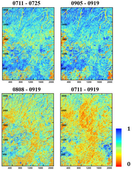
Figure 16.
Coherence images for different interferometric data; 0711-0725 and 0905-0919 data sets have higher coherence, 0808-0919 data set has lower coherence, and 0711-0919 data set has the lowest coherence. The data with larger temporal baselines have lower coherence, and temporal decorrelation decreases the coherence. The spatial distribution of coherence is not uniform and receives a combination of volume decorrelation and temporal decorrelation.
Figure 17 shows the forest height inversion results of the improved model with different interference datasets. The inversion results show that the improved inversion method is robust for the forest height inversion under different and temporal baselines. Although there was some biasness between the data sets, this error may have been influenced by abrupt changes in the ground phase in addition to the reasons mentioned in Section 5. Moreover, the inversion effect does not decrease significantly for the data sets 0808-0919 and 0711-0919 with larger temporal baselines. The temporal baseline of the 0711-0919 data set was found to be larger, and it showed a better inversion effect than 0808-0919. This could be because the difference in the coherence between the two sets of data were little. Meanwhile, the data are less sensitive to temporal decorrelation interference due to the large original of 0711-0919 data, resulting in the preference in the overall inversion result. Therefore, for repeat-pass spaceborne PolInSAR, the improved model can be relatively robust to forest height inversion.

Figure 17.
Inversion of forest height using different data.
6.2. Error Analysis of Inversion Results
Errors in the inversion results and the effect of residual temporal decorrelation on the model are the common factors that affect the accuracy of the inversion results. However, other factors outside the model may also cause the problem of accuracy degradation. This study was based on the assumption of the traditional three-stage method [38]. Besides the temporal decorrelation source, the inversion results are still faced with two aspects of errors: residual ground contribution in the volume scattering complex coherence and the estimated shift of the real ground phase [63]. The inversion process usually assumes that the ground scattering contribution of volume-only scattering complex coherence is 0. However, when there is a strong interaction at the dihedral angle of the earth, the polarization channels with low ground contribution will still be affected by the ground scattering center, increasing the variance of the inversion results. Thus, the accuracy of the fitting is reduced [38].
Previous studies have attempted to optimize this phenomenon and can be categorized into three groups based on their principles: separation of the contribution of volume scattering based on polarization decomposition [8,64], optimization by coherence to minimize the effect of ground scattering contributions [39,45,65], and methods that introduce other data sources, such as different baselines [66], and different frequency bands [67,68]. At present, these methods can only reduce the error of ground contribution to a certain extent. Based on the repeat-pass spaceborne PolInSAR data with low coherence, the improved model introduces partial coherence optimization to help in the model calculation. This method is very valuable in research. However, removal of ground contribution to the inversion effect deserves further in-depth study.
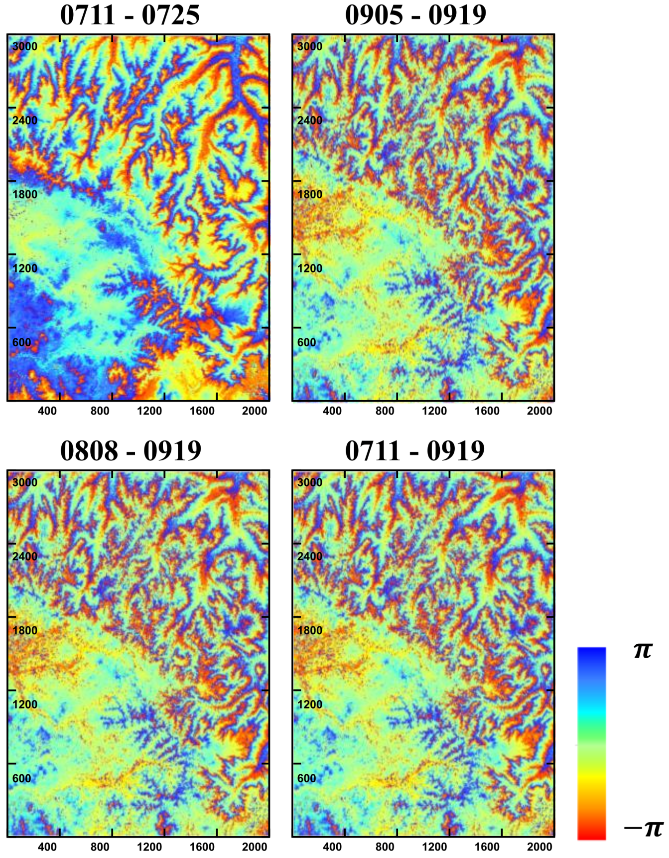
Even after terrain correction, the influence of ground phase estimation is still inevitable [11]. The ground phase images were estimated from different interferometric data during the three-stage inversion (Figure 18). The ground phase of all interferometric pairs, as distinguished from the interferometric DEM (Figure 4c), was affected by abrupt changes resulting to incorrect ground point selection during the inversion. The phase error was particularly prominent in 0711-0725, where the of this data set was smaller than the other groups. Thus, the spatial baseline of this data set was shorter than the other groups during interferometry. In addition, the abrupt changes of terrain phase were more obvious in rugged terrain, which was consistent with previous findings [69]. In contrast, the abrupt ground phase error for 0711-0919 was not significant, indicating that the estimation error of the ground phase was not significantly affected by the temporal baseline when compared to spatial baseline. This also supported previous conclusions about the same [32,61].
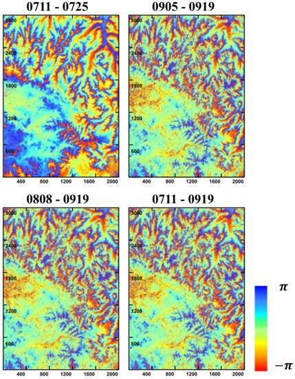
Figure 18.
Phase estimation of three-stage inversion method for different interferometric pairs. There are relatively obvious phase point anomalies in the estimates of 0711-0725, which are more evident in the rugged terrain type (upper right corner). Thus, it can be demonstrated that the interferometric data with shorter spatial baselines are more prone to errors in the ground phase estimates.
The forest average height serves as the standard forestry table measurement parameter and plays an important role in forest inventory and subsequent biomass estimation [70]. However, it has also been suggested that forest dominance height is closer to the effective height of the remote sensing signal [63], and the difference tends to be more pronounced for forests with lower heights. In addition, differences in forest species and density may also have an impact on the inversion results. The reasons are mainly the differences arising from the canopy cover and the ratio of canopy to bare ground. In the general boreal temperate forests of China, the distribution of forest species and density is complex. They were not strictly classified and studied separately in this study. This will undoubtedly have some influence on the inversion accuracy, which is worthy of our further study. It is worth noting that although the sample size does not bias the fit results, it may still cause a reduction in correlation [52].
The model proposed in this study is only for the fuzzy inversion of forest height caused by temporal decorrelation. It does not focus on the inversion errors caused by other factors that may exist. As such, the model is only suitable for data whose main error source is temporal decorrelation. In addition, this study is a regional study, and the model has only been verified in the height inversion of forests in northern China. Therefore, the inversion of the model in other regional forests requires further studies.
6.3. Suitable Range of Spatial Baseline for Forest Height Inversion
In this study, height inversion of repeat-pass spaceborne PolInSAR data revealed that the degree of influence of temporal decorrelation on the inversion accuracy depends not only on the length of the temporal baseline, but also on the sensitivity of the data to temporal decorrelation, such as the magnitude of . Given the upcoming large-scale forest biomass observation mission, the multifaceted parameters of PolInSAR data should be carefully considered. The spaceborne SAR sensor has a relatively fixed flight trajectory when compared to the airborne SAR, and it is relatively difficult to change its space parameters. Therefore, this study aims at providing more insights about the spatial parameter suitable for the forest height of the spaceborne SAR inversion. This will help future studies in establishing a suitable spaceborne inversion system.
Given the sensitivity of the ground target height to the interferometric phase, the phase shift caused by temporal decorrelation causes the most interference to the forest height calculation. Therefore, the correction term in the model (Equation (23)) has the most significant impact on the inversion accuracy. In Equation (23), the function of the parameter is to correct the phase deviation. However, from another perspective, the inversion accuracy can be measured by converting to the size of . As such, the inversion accuracy can be improved by using the data suitable for .
In this study, we used L-band ALOS2 repeat-pass spaceborne PolInSAR data to retrieve the height of temperate forest in the Saihanba region of northern China, and obtained the parameters under different and temporal baselines. When the value of the spaceborne data reached of the corresponding height, the data were considered suitable for inversion of the forest height using the polarized interferometric model. The suitable for different data pairs can be obtained from Table 2 and Table 3, as shown in Table 5.

Table 5.
Suitable for different data pairs.
The analysis of Table 5 shows that a larger vertical baseline is more suitable for repeat-pass spaceborne PolInSAR inversion of forest height, and a similar conclusion was reached in a previous study upon analysis of airborne data [11,50]. This is because when the is larger, the baseline decorrelation caused by the spatial baseline between the primary and secondary images is greater. The larger results obtained in the study indicate that the disturbance caused by baseline decorrelation can be hardly considered when compared to temporal decorrelation. Conversely, smaller may cause abrupt changes in the phase estimation of the underlying surface, causing a decrease in the inversion accuracy. In addition, the suitable of different temporal baselines slightly differed for the same area data, indicating that the sensitivity of to temporal decorrelation is more important than that of temporal baseline. Therefore, more attention should be paid to the use of suitable when using repeat-pass spaceborne SAR data interferometry to measure forest height.
However, according to previous studies, the choice of was negatively correlated to the forest height in the observation area [11]. The value could be appropriately lowered when the forest height of the study area was higher. According to the average forest height in this study, the suitable exceeded the fuzzy interval of . Since the relationship between of the data and the ground height has to be within the fuzzy interval, there may not be a suitable value of for inversion if the inversion model is not improved. Therefore, the correction of the parameter for the phase is essential when the temporal decorrelation of the data has a significant effect.
7. Conclusions
The performance study of forest height through repeat-pass spaceborne PolInSAR inversion will effectively improve large-scale forest height estimation efficiency. To address the limitations of the current inversion of forest height with repeat-pass L-band spaceborne PolInSAR data, a theoretical analysis of the effects of phase deviation and temporal decorrelation on the inversion performance and an improved inversion method are proposed based on the RVoG model. In this respect, this study makes three main conclusions: (1) the correction of temporal decorrelation can improve the robustness and accuracy of the forest height inversion. (2) A more accurate forest height inversion of common SAR data can be performed using the improved model, but there may still be a small degree of error in the inversion results. (3) Data with large temporal baselines should be carefully selected when using models for height inversion.
The repeat-pass spaceborne sensors have a more extended temporal baseline than the airborne sensors, which exposes the repeat-pass spaceborne PolInSAR to more excellent decorrelation effects when inverting forest heights in the study area. Besides, the vertical wavenumber of the repeat-pass spaceborne sensor is lower than the interval suitable for inversion, making the inversion height more sensitive to decorrelation. When affected by these two factors, the spaceborne PolInSAR data often loses the ability to invert the forest height using the traditional three-stage inversion method.
To avoid the interference of both factors as much as possible, we propose a semi-empirical improvement model that controls the iterations by ground true data, based on the three-stage inversion method. Through theoretical analysis, it was found that in general cases, there is a correction term to make the error between the inversion results and the true value to converge to less than 15%. Moreover, there is more than one correction term for any reasonable range of specified forest height and can accurately invert the forest height under the influence of temporal decorrelation.
This method uses ALOS2 repeat-pass spaceborne L-band PolInSAR data with large temporal baseline to perform accurate forest height inversion in the mixed conifer-broad forest of the Saihanba of northern China. For different interferometric pairs, the RMSEs of inversion results were less than 15%. For the interferometric data of the larger temporal baseline, the inversion results were slightly lower than other interferometric pairs because of the low coherence caused by decorrelation. Nevertheless, this study is based on the assumptions of the traditional three-stage inversion method. Therefore, there is need for further research to improve the accuracy of this method using previous improved models, such as ground contribution and terrain impact.
The present study achieves adequate accuracy in forest height inversion by repeat-pass spaceborne PolInSAR data through the improved model. However, accuracy degradation may occur during inversion of heterogeneous forests because the results are affected by height variation. Further research is therefore needed to establish whether general patterns can be summarized to avoid the above problems by examining data from different forest height intervals.
Author Contributions
Conceptualization, W.F. and Y.Y.; investigation, A.S., Z.L., G.W.; experimentation, data processing, validation, and manuscript writing, Y.M.; editing, O.O.M. All authors have read and agreed to the published version of the manuscript.
Funding
This research was funded by the National Natural Science Foundation of China (contract no. 31971654) and the Civil Aerospace Technology Advance Research Project (contract no. D040114).
Data Availability Statement
Data was obtained from the Japan Aerospace Exploration Agency and are available at https://www.eorc.jaxa.jp/ALOS-2/en/about/palsar2.htm (accessed on 12 September 2021).
Conflicts of Interest
The funders had no role in the design of the study; in the collection, analyses, or interpretation of data; in the writing of the manuscript, or in the decision to publish the results.
References
- Purves, D.; Pacala, S. Forests in Flux. Science 2013, 342, 776. [Google Scholar] [CrossRef]
- Hall, F.G.; Bergen, K.; Blair, J.B.; Dubayah, R.; Houghton, R.; Hurtt, G.; Kellndorfer, J.; Lefsky, M.; Ranson, J.; Saatchi, S.; et al. Characterizing 3D vegetation structure from space: Mission requirements. Remote Sens. Environ. 2011, 115, 2753–2775. [Google Scholar] [CrossRef] [Green Version]
- Houghton, R.A.; Hall, F.; Goetz, S. Importance of biomass in the global carbon cycle. J. Geophys. Res. Space Phys. 2009, 114, 302. [Google Scholar] [CrossRef]
- Lei, Y.; Treuhaft, R.; Gonçalves, F. Automated estimation of forest height and underlying topography over a Brazilian tropical forest with single-baseline single-polarization TanDEM-X SAR interferometry. Remote Sens. Environ. 2021, 252, 112132. [Google Scholar] [CrossRef]
- Gu, C.; Clevers, J.G.; Liu, X.; Tian, X.; Li, Z.; Li, Z. Predicting forest height using the GOST, Landsat 7 ETM+, and airborne LiDAR for sloping terrains in the Greater Khingan Mountains of China. ISPRS J. Photogramm. Remote Sens. 2018, 137, 97–111. [Google Scholar] [CrossRef]
- Huang, H.; Liu, C.; Wang, X.; Biging, G.S.; Chen, Y.; Yang, J.; Gong, P. Mapping vegetation heights in China using slope correction ICESat data, SRTM, MODIS-derived and climate data. ISPRS J. Photogramm. Remote Sens. 2017, 129, 189–199. [Google Scholar] [CrossRef]
- Schlund, M.; Baron, D.; Magdon, P.; Erasmi, S. Canopy penetration depth estimation with TanDEM-X and its compensation in temperate forests. ISPRS J. Photogramm. Remote Sens. 2019, 147, 232–241. [Google Scholar] [CrossRef]
- Aghabalaei, A.; Ebadi, H.; Maghsoudi, Y. Forest height estimation based on the RVoG inversion model and the PolInSAR decomposition technique. Int. J. Remote Sens. 2019, 41, 2684–2703. [Google Scholar] [CrossRef]
- Hajnsek, I.; Kugler, F.; Lee, S.-K.; Papathanassiou, K.P. Tropical-Forest-Parameter Estimation by Means of Pol-InSAR: The INDREX-II Campaign. IEEE Trans. Geosci. Remote Sens. 2009, 47, 481–493. [Google Scholar] [CrossRef] [Green Version]
- Koch, B. Status and future of laser scanning, synthetic aperture radar and hyperspectral remote sensing data for forest biomass assessment. ISPRS J. Photogramm. Remote Sens. 2010, 65, 581–590. [Google Scholar] [CrossRef]
- Liao, Z.; He, B.; van Dijk, A.I.; Bai, X.; Quan, X. The impacts of spatial baseline on forest canopy height model and digital terrain model retrieval using P-band PolInSAR data. Remote Sens. Environ. 2018, 210, 403–421. [Google Scholar] [CrossRef]
- Wang, M.; Sun, R.; Xiao, Z. Estimation of Forest Canopy Height and Aboveground Biomass from Spaceborne LiDAR and Landsat Imageries in Maryland. Remote Sens. 2018, 10, 344. [Google Scholar] [CrossRef] [Green Version]
- Huang, H.; Liu, C.; Wang, X.; Zhou, X.; Gong, P. Integration of multi-resource remotely sensed data and allometric models for forest aboveground biomass estimation in China. Remote Sens. Environ. 2019, 221, 225–234. [Google Scholar] [CrossRef]
- Liao, Z.; He, B.; Quan, X.; van Dijk, A.I.; Qiu, S.; Yin, C. Biomass estimation in dense tropical forest using multiple information from single-baseline P-band PolInSAR data. Remote Sens. Environ. 2019, 221, 489–507. [Google Scholar] [CrossRef]
- Ferretti, A.; Prati, C.; Rocca, F. Nonlinear subsidence rate estimation using permanent scatterers in differential SAR interferometry. IEEE Trans. Geosci. Remote Sens. 2000, 38, 2202–2212. [Google Scholar] [CrossRef] [Green Version]
- Graham, L.C. Synthetic interferometer radar for topographic mapping. Proc. IEEE 1974, 62, 763–768. [Google Scholar] [CrossRef]
- Huang, L.; Hajnsek, I. Polarimetric Behavior for the Derivation of Sea Ice Topographic Height From TanDEM-X Interferometric SAR Data. IEEE J. Sel. Top. Appl. Earth Obs. Remote Sens. 2021, 14, 1095–1110. [Google Scholar] [CrossRef]
- Schlund, M.; von Poncet, F.; Hoekman, D.H.; Kuntz, S.; Schmullius, C. Importance of Bistatic SAR Features from TanDEM-X for Forest Mapping and Monitoring. Remote Sens. Environ. 2014, 151, 16–26. [Google Scholar] [CrossRef]
- Zhang, L.; Duan, B.; Zou, B. Research on Inversion Models for Forest Height Estimation Using Polarimetric SAR Interferometry. Int. Arch. Photogramm. Remote Sens. Spatial Inf. Sci. 2017, 42, 659–663. [Google Scholar] [CrossRef] [Green Version]
- Garestier, F.; le Toan, T. Forest Modeling for Height Inversion Using Single-Baseline InSAR/Pol-InSAR Data. IEEE Trans. Geosci. Remote Sens. 2010, 48, 1528–1539. [Google Scholar] [CrossRef]
- Askne, J.; Santoro, M.; Smith, G.; Fransson, J. Multitemporal repeat-pass sar interferometry of boreal forests. IEEE Trans. Geosci. Remote Sens. 2003, 41, 1540–1550. [Google Scholar] [CrossRef]
- Askne, J.I.; Soja, M.J.; Ulander, L.M. Biomass estimation in a boreal forest from TanDEM-X data, lidar DTM, and the interferometric water cloud model. Remote Sens. Environ. 2017, 196, 265–278. [Google Scholar] [CrossRef]
- Hagberg, J.; Ulander, L.M.H.; Askne, J. Repeat-pass SAR interferometry over forested terrain. IEEE Trans. Geosci. Remote Sens. 1995, 33, 331–340. [Google Scholar] [CrossRef]
- Zhang, B.; Fu, H.; Zhu, J.; Peng, X.; Xie, Q.; Lin, D.; Liu, Z. A Multibaseline PolInSAR Forest Height Inversion Model Based on Fourier–Legendre Polynomials. IEEE Geosci. Remote Sens. Lett. 2021, 18, 687–691. [Google Scholar] [CrossRef]
- Cloude, S.; Papathanassiou, K. Polarimetric SAR interferometry. IEEE Trans. Geosci. Remote Sens. 1998, 36, 1551–1565. [Google Scholar] [CrossRef]
- Treuhaft, R.N.; Madsen, S.N.; Moghaddam, M.; van Zyl, J.J. Vegetation characteristics and underlying topography from interferometric radar. Radio Sci. 1996, 31, 1449–1485. [Google Scholar] [CrossRef]
- Treuhaft, R.N.; Siqueira, P.R. Vertical structure of vegetated land surfaces from interferometric and polarimetric radar. Radio Sci. 2000, 35, 141–177. [Google Scholar] [CrossRef] [Green Version]
- Soja, M.J.; Persson, H.; Ulander, L.M.H. Estimation of Forest Height and Canopy Density From a Single InSAR Correlation Coefficient. IEEE Geosci. Remote Sens. Lett. 2014, 12, 646–650. [Google Scholar] [CrossRef] [Green Version]
- Fu, H.; Wang, C.; Zhu, J.; Xie, Q.; Zhang, B. Estimation of Pine Forest Height and Underlying DEM Using Multi-Baseline P-Band PolInSAR Data. Remote Sens. 2016, 8, 820. [Google Scholar] [CrossRef] [Green Version]
- Xie, Q.; Zhu, J.; Wang, C.; Fu, H.; Lopez-Sanchez, J.M.; Ballester-Berman, J.D. A Modified Dual-Baseline PolInSAR Method for Forest Height Estimation. Remote Sens. 2017, 9, 819. [Google Scholar] [CrossRef] [Green Version]
- Cloude, S.R. Robust parameter estimation using dual baseline polarimetric SAR interferometry. In Proceedings of the IEEE International Geoscience and Remote Sensing Symposium, Toronto, ON, Canada, 24–28 June 2002; IEEE: Piscataway, NJ, USA, 2003; Volume 2, pp. 838–840. [Google Scholar]
- Lavalle, M.; Hensley, S. Extraction of Structural and Dynamic Properties of Forests From Polarimetric-Interferometric SAR Data Affected by Temporal Decorrelation. IEEE Trans. Geosci. Remote Sens. 2015, 53, 4752–4767. [Google Scholar] [CrossRef]
- Lu, H.; Suo, Z.; Guo, R.; Bao, Z. S-RVoG model for forest parameters inversion over underlying topography. Electron. Lett. 2013, 49, 618–620. [Google Scholar] [CrossRef]
- Ghasemi, N.; Tolpekin, V.; Stein, A. A modified model for estimating tree height from PolInSAR with compensation for temporal decorrelation. Int. J. Appl. Earth Obs. Geoinf. 2018, 73, 313–322. [Google Scholar] [CrossRef]
- Cloude, S.R.; Williams, M.L. A coherent EM scattering model for dual baseline POLInSAR. In Proceedings of the 2003 IEEE International Geoscience and Remote Sensing Symposium, Toulouse, France, 21–25 July 2003; IEEE: Piscataway, NJ, USA, 2004; Volume 3, pp. 1423–1425. [Google Scholar]
- Managhebi, T.; Maghsoudi, Y.; Zoej, M.J.V. A Volume Optimization Method to Improve the Three-Stage Inversion Algorithm for Forest Height Estimation Using PolInSAR Data. IEEE Geosci. Remote Sens. Lett. 2018, 15, 1214–1218. [Google Scholar] [CrossRef]
- Chen, W.; Zheng, Q.; Xiang, H.; Chen, X.; Sakai, T. Forest Canopy Height Estimation Using Polarimetric Interferometric Synthetic Aperture Radar (PolInSAR) Technology Based on Full-Polarized ALOS/PALSAR Data. Remote Sens. 2021, 13, 174. [Google Scholar] [CrossRef]
- Shi, Y.; He, B.; Liao, Z. An improved dual-baseline PolInSAR method for forest height inversion. Int. J. Appl. Earth Obs. Geoinf. 2021, 103, 102483. [Google Scholar] [CrossRef]
- Xing, C.; Zhang, T.; Wang, H.; Zeng, L.; Yin, J.; Yang, J. A Novel Four-Stage Method for Vegetation Height Estimation with Repeat-Pass PolInSAR Data via Temporal Decorrelation Adaptive Estimation and Distance Transformation. Remote Sens. 2021, 13, 213. [Google Scholar] [CrossRef]
- Ahmed, R.; Siqueira, P.; Hensley, S.; Chapman, B.; Bergen, K. A survey of temporal decorrelation from spaceborne L-Band repeat-pass InSAR. Remote Sens. Environ. 2011, 115, 2887–2896. [Google Scholar] [CrossRef]
- Lee, S.-K.; Kugler, F.; Papathanassiou, K.; Hajnsek, I. Quantification and compensation of temporal decorrelation effects in polarimetric SAR interferometry. In Proceedings of the 2012 IEEE International Geoscience and Remote Sensing Symposium, Munich, Germany, 22–27 July 2012; IEEE: Piscataway, NJ, USA, 2012; pp. 3106–3109. [Google Scholar]
- Lei, Y.; Siqueira, P. Estimation of Forest Height Using Spaceborne Repeat-Pass L-Band InSAR Correlation Magnitude over the US State of Maine. Remote Sens. 2014, 6, 10252–10285. [Google Scholar] [CrossRef] [Green Version]
- Lavalle, M.; Simard, M.; Hensley, S. A Temporal Decorrelation Model for Polarimetric Radar Interferometers. IEEE Trans. Geosci. Remote Sens. 2011, 50, 2880–2888. [Google Scholar] [CrossRef]
- Neumann, M.; Ferro-Famil, L.; Reigber, A. Estimation of Forest Structure, Ground, and Canopy Layer Characteristics from Multibaseline Polarimetric Interferometric SAR Data. IEEE Trans. Geosci. Remote Sens. 2009, 48, 1086–1104. [Google Scholar] [CrossRef] [Green Version]
- Papathanassiou, K.; Cloude, S. The effect of temporal decorrelation on the inversion of forest parameters from Pol-InSAR data. In Proceedings of the IGARSS 2003, 2003 IEEE International Geoscience and Remote Sensing Symposium, Toulouse, France, 21–25 July 2003; IEEE: Piscataway, NJ, USA, 2004; Volume 3, pp. 1429–1431. [Google Scholar]
- Simard, M.; Denbina, M. An Assessment of Temporal Decorrelation Compensation Methods for Forest Canopy Height Estimation Using Airborne L-Band Same-Day Repeat-Pass Polarimetric SAR Interferometry. IEEE J. Sel. Top. Appl. Earth Obs. Remote Sens. 2018, 11, 95–111. [Google Scholar] [CrossRef]
- Lee, S.-K.; Fatoyinbo, T.; Osmanoğlu, B.; Sun, G. Polarimetric SAR interferometry evaluation in mangroves. In Proceedings of the 2014 IEEE Geoscience and Remote Sensing Symposium, Quebec City, QC, Canada, 13–18 July 2014; IEEE: Piscataway, NJ, USA, 2014; pp. 4584–4587. [Google Scholar]
- Lei, Y.; Siqueira, P.; Torbick, N.; Ducey, M.; Chowdhury, D.; Salas, W. Generation of Large-Scale Moderate-Resolution Forest Height Mosaic With Spaceborne Repeat-Pass SAR Interferometry and Lidar. IEEE Trans. Geosci. Remote Sens. 2018, 57, 770–787. [Google Scholar] [CrossRef]
- Kugler, F.; Lee, S.-K.; Hajnsek, I.; Papathanassiou, K.P. Forest Height Estimation by Means of Pol-InSAR Data Inversion: The Role of the Vertical Wavenumber. IEEE Trans. Geosci. Remote Sens. 2015, 53, 5294–5311. [Google Scholar] [CrossRef]
- Du, K.; Lin, H.; Wang, G.; Long, J.; Li, J.; Liu, Z. The Impact of Vertical Wavenumber on Forest Height Inversion by PolInSAR. In Proceedings of the 2018 Fifth International Workshop on Earth Observation and Remote Sensing Applications (EORSA), Xi’an, China, 18–20 June 2018; IEEE: Piscataway, NJ, USA, 2018; pp. 1–5. [Google Scholar]
- Jiang, L.; Wang, J.; Cui, H.; Wang, G.; Zhao, T.; Zhao, S.; Chai, L.; Liu, X.; Yang, J. In situ soil moisture and temperature network in genhe watershed and saihanba area in China. Data Brief 2020, 31, 105693. [Google Scholar] [CrossRef]
- Hosseini, S.; Garestier, F. Pol-InSAR sensitivity to hemi-boreal forest structure at L- and P-bands. Int. J. Appl. Earth Obs. Geoinf. 2021, 94, 102213. [Google Scholar] [CrossRef]
- Gatelli, F.; Guamieri, A.M.; Parizzi, F.; Pasquali, P.; Prati, C.; Rocca, F. The wavenumber shift in SAR interferometry. IEEE Trans. Geosci. Remote Sens. 1994, 32, 855–865. [Google Scholar] [CrossRef] [Green Version]
- Zebker, H.; Villasenor, J. Decorrelation in interferometric radar echoes. IEEE Trans. Geosci. Remote Sens. 1992, 30, 950–959. [Google Scholar] [CrossRef] [Green Version]
- Gomba, G.; Parizzi, A.; De Zan, F.; Eineder, M.; Bamler, R. Toward Operational Compensation of Ionospheric Effects in SAR Interferograms: The Split-Spectrum Method; IEEE: Piscataway, NJ, USA, 2016; Volume 54, pp. 1446–1461. [Google Scholar]
- Liang, C.; Fielding, E.J. Measuring Azimuth Deformation with L-Band ALOS-2 ScanSAR Interferometry. IEEE Trans. Geosci. Remote Sens. 2017, 55, 2725–2738. [Google Scholar] [CrossRef] [Green Version]
- Shimada, M.; Isoguchi, O.; Tadono, T.; Isono, K. PALSAR Radiometric and Geometric Calibration. IEEE Trans. Geosci. Remote Sens. 2009, 47, 3915–3932. [Google Scholar] [CrossRef]
- Woods, J.W.; Biemond, J. Comments on “A Model for Radar Images and Its Application to Adaptive Digital Filtering of Multiplicative Noise”. IEEE Trans. Pattern Anal. Mach. Intell. 1984, PAMI-6, 658–659. [Google Scholar] [CrossRef]
- Rosen, P.A.; Hensley, S.; Joughin, I.R.; Li, F.K.; Madsen, S.N.; Rodriguez, E.; Goldstein, R.M. Synthetic aperture radar interferometry. Proc. IEEE 2000, 88, 333–380. [Google Scholar] [CrossRef]
- Cloude, S.; Papathanassiou, K. Three-stage inversion process for polarimetric SAR interferometry. IEE Proc.-Radar Sonar Navig. 2003, 150, 125–134. [Google Scholar] [CrossRef] [Green Version]
- Lei, Y.; Siqueira, P. An Automatic Mosaicking Algorithm for the Generation of a Large-Scale Forest Height Map Using Spaceborne Repeat-Pass InSAR Correlation Magnitude. Remote Sens. 2015, 7, 5639–5659. [Google Scholar] [CrossRef] [Green Version]
- Thiel, C.; Schmullius, C. Investigating ALOS PALSAR Interferometric Coherence in Central Siberia at Unfrozen and Frozen Conditions: Implications for Forest Growing Stock Volume Estimation. Can. J. Remote Sens. 2013, 39, 232–250. [Google Scholar] [CrossRef]
- Mette, T.; Kugler, F.; Papathanassiou, K.; Hajnsek, I. Forest and the Random Volume over Ground—Nature and Effect of 3 Possible Error Types. In Proceedings of the European Conference on Synthetic Aperture Radar (EUSAR), Hamburg, Germany, 6–9 June 2016; pp. 1–4. [Google Scholar]
- Ballester-Berman, J.D.; Lopez-Sanchez, J.M. Applying the Freeman–Durden Decomposition Concept to Polarimetric SAR Interferometry. IEEE Trans. Geosci. Remote Sens. 2010, 48, 466–479. [Google Scholar] [CrossRef]
- Xie, Q.; Zhu, J.; Wang, C.; Fu, H. Boreal forest height inversion using E-SAR PolInSAR data based coherence optimization methods and three-stage algorithm. In Proceedings of the 2014 Third International Workshop on Earth Observation and Remote Sensing Applications (EORSA), Changsha, China, 11–14 June 2014; IEEE: Piscataway, NJ, USA, 2014; pp. 145–150. [Google Scholar] [CrossRef]
- Babu, A.; Kumar, S. TREE CANOPY HEIGHT ESTIMATION USING MULTI BASELINE RVOG INVERSION TECHNIQUE. ISPRS Int. Arch. Photogramm. Remote Sens. Spat. Inf. Sci. 2018, XLII-5, 605–611. [Google Scholar] [CrossRef] [Green Version]
- Khati, U.; Singh, G.; Kumar, S. Potential of Space-Borne PolInSAR for Forest Canopy Height Estimation over India—A Case Study Using Fully Polarimetric L-, C- and X-Band SAR Data. IEEE J. Sel. Top. Appl. Earth Obs. Remote Sens. 2018, 11, 2406–2416. [Google Scholar] [CrossRef]
- Li, X.; Guo, H.; Li, Z.; Wang, L. Inversion of vegetation height using SIR-C dual frequency polarimetric sar interferometry data. In Proceedings of the IEEE International Geoscience and Remote Sensing Symposium, Anchorage, AK, USA, 20–24 September 2004; IEEE: Piscataway, NJ, USA, 2004; Volume 5, pp. 3132–3135. [Google Scholar] [CrossRef]
- Le Toan, T.; Quegan, S.; Davidson, M.; Balzter, H.; Paillou, P.; Papathanassiou, K.; Plummer, S.; Rocca, F.; Saatchi, S.; Shugart, H.; et al. The BIOMASS mission: Mapping global forest biomass to better understand the terrestrial carbon cycle. Remote Sens. Environ. 2011, 115, 2850–2860. [Google Scholar] [CrossRef] [Green Version]
- Mette, T.; Papathanassiou, K.; Hajnsek, I.; Zimmermann, R. Forest biomass estimation using polarimetric SAR interferometry. In Proceedings of the IEEE International Geoscience and Remote Sensing Symposium, Toronto, ON, Canada, 24–28 June 2002; IEEE: Piscataway, NJ, USA, 2002; Volume 2, pp. 817–819. [Google Scholar] [CrossRef]
Publisher’s Note: MDPI stays neutral with regard to jurisdictional claims in published maps and institutional affiliations. |
© 2021 by the authors. Licensee MDPI, Basel, Switzerland. This article is an open access article distributed under the terms and conditions of the Creative Commons Attribution (CC BY) license (https://creativecommons.org/licenses/by/4.0/).

