Article

Evaluating the Farmland Use Intensity and Its Patterns in a Farming—Pastoral Ecotone of Northern China

1
College of Land Science and Technology, China Agricultural University, Beijing 100193, China
2
Ministry of Education Key Laboratory for Earth System Modeling, Department of Earth System Science, Tsinghua University, Beijing 100084, China
3
Centre for Earth Observation Sciences, Department of Earth and Atmospheric Sciences, University of Alberta, Edmonton, AB T6G 2E3, Canada
4
College of Engineering, South China Agricultural University, Guangzhou 510642, China
5
College of Resources and Environmental Science, China Agricultural University, Beijing 100193, China
*
Author to whom correspondence should be addressed.
Remote Sens. 2021, 13(21), 4304; https://doi.org/10.3390/rs13214304
Submission received: 22 September 2021 / Revised: 21 October 2021 / Accepted: 23 October 2021 / Published: 26 October 2021
(This article belongs to the Special Issue Advances in Remote Sensing for Crop Monitoring and Yield Estimation)

Abstract

:
The growing population and northward shifts in the center of grain production collectively contribute to the arising farmland use intensity of the farming–pastoral ecotone of Northern China (FPENC). Consequently, it poses a great threat to the vulnerable ecosystem of FPENC. Thus, farmland use intensity monitoring is a top priority to practice sustainable farming. In this study, we establish an indicator system designed to evaluate farmland use intensity in Ulanqab, located in the central part of FPENC. This system includes three single-year indicators (the degree of coupling between effective rainfall and crop water requirement (Dcrr), irrigation intensity (Iri) and crop duration (Cd)) and two multi-year indicators (the frequency of adopting the green-depressing cropping system (Gf) and rotation frequency (Rf)). We mapped five farmland use intensity indicators in Ulanqab from 2010 to 2019 using satellite imagery and other ancillary data. Then, the farmland use patterns were recognized by applying the self-organizing map algorithm. Our results suggest that the mapping results of crop types, center pivot irrigation (CPI), and irrigated areas are reasonably accurate. Iri, Cd, and Rf experienced an increase of 31 m3/hm2, 1 day, and 0.06 in Ulanqab from 2010 to 2019, respectively, while Dcrr and Gf witnessed a decrease of 0.002 and 0.004, respectively. That is, farmers are progressively inclined to higher farmland use intensity. Moreover, spatial heterogeneity analysis shows that Northern Ulanqab owned higher Dcrr, Iri, Cd, and Rf, and lower Gf than the southern part. We conclude the paper by discussing the implications of the results for areas with different farmland use intensity patterns.

Graphical Abstract

1. Introduction

The food demand for agricultural products in China will increase over the coming decades, driven by a growing population [1,2], which means that agricultural production will increase. Rising farmland use intensity has contributed greatly to alleviating arable land scarcity and improving food security [3]. However, there are concerns over the long-term sustainability of excessive agricultural intensification [4,5]. A large and growing body of literature has investigated the negative impacts of this phenomenon, e.g., soil erosion [6], biodiversity loss [6,7,8], declining groundwater table [9,10] and desertification [11]. This is particularly the case in arid and semi-arid areas, such as in the farming–pastoral ecotone of Northern China (FPENC), which has a highly sensitive and vulnerable ecosystem [12,13]. A crucial precondition for the development of strategies for sustainable intensification is knowledge about the farmland use intensity patterns [14].
Farmland use intensity has been regarded as a measure for revealing the level of agricultural development, however, there is a lack of a commonly shared practical definition in practice [15]. This dilemma may partly be because of the measurement of farmland use intensity for different purposes [16,17]. Brookfield (1972) described farmland use intensity as the inputs of capital, labor, and skills for a given land in a traditional economic view [18], whereas Dietrich (2012) used a formulation that agricultural land-use intensity is “the degree of yield amplification caused by human activities” [19]. It follows that farmland use intensity is traditionally defined from agricultural input or output perspectives. Given this, scholars have further proposed to subdivide farmland use intensity into input and output intensity [14,20]. Farmland use intensity can be evaluated either in an output-oriented or input-oriented way by using inputs as surrogates for productivity increases [19]. Meanwhile, from a geographical perspective, utilization degree -related measures, including crop patterns, cropping frequency [3,21], crop rotation [22], fallow cycle [23], and crop duration ratio [24], are also frequently reported to represent the intensity of agricultural activities [25]. In general, metrics concerning the utilization degree have been proven to be promising and reliable for the assessment of farmland use intensity [26].
Statistical data are commonly adopted to quantify farmland use intensity, using parameters such as fertilizer, pesticide, machinery and labor use, and the number of harvests per year [27,28,29,30]. Normally, these data are recorded at aggregated spatial scales such as at city-level or county-level. In general, averages at a regional scale are too coarse to capture the great spatial heterogeneity of farmland use intensity within a single administrative region [31] or to support field-level decision making. This applies to countries such as China, where the government allocates farmlands to individual rural households using a household responsibility system. The said system gives farmers the right to make independent decisions on small pieces of contracted land [32]. Consequently, farmland use practices vary considerably between plots within a given statistical unit. In addition, the different statistical standards and adjustments of administrative divisions can raise many uncertainties in such contexts. Therefore, farmland use intensity maps with a higher spatial resolution are required [33]. In this context, remote sensing technology has become the most widely adopted method to acquire indicators of farmland use intensity [34,35].
Over the last several decades, many existing studies have highlighted the potential of satellite imagery to identify single cropping practices at various spatial scales. For example, Zhong et al. (2019) developed a deep learning method to classify various summer crops of Yolo County, California, employing the Landsat Enhanced Vegetation index [36]. Based on an extensive crop sequence dataset, Waldhoff et al. (2017) further derived the crop rotation schemes of the Ruhr catchment in Germany [22]. Marshall et al. (2011) demonstrated the ability of high-resolution satellite imagery for crop area monitoring in Niger [37]. Bolton and Friedl (2013) showed that remotely sensed vegetation indices perform well in estimating crop yields in Central United States [38]. Ambika et al. (2016) developed high-resolution irrigated area maps with satisfactory accuracy for Indian agroecological areas by applying remote sensing data [39]. Importantly, the above-mentioned studies based on remote sensing products conventionally involved evaluating farmland use intensity using a single indicator only. Nonetheless, agricultural systems are highly heterogeneous and complex [25], and one single indicator alone is not enough to describe all aspects of farmland use intensity.
Based on statistical data, some scholars have attempted to apply multivariate statistical analyses, such as the principal component analysis [40], multi-objective comprehensive evaluation method [41], hierarchical approach [42], and fuzzy cognitive mapping [43]. Such methods are highly expert knowledge-driven, which reduces the objectivity of the evaluation of farmland use intensity. Considering the restrictions of the above methods, we employed a self-organizing map (SOM), a neural network-based dimensionality reduction algorithm [43,44,45], to convert a high-dimensional indicator system into a two-dimensional cropping pattern.
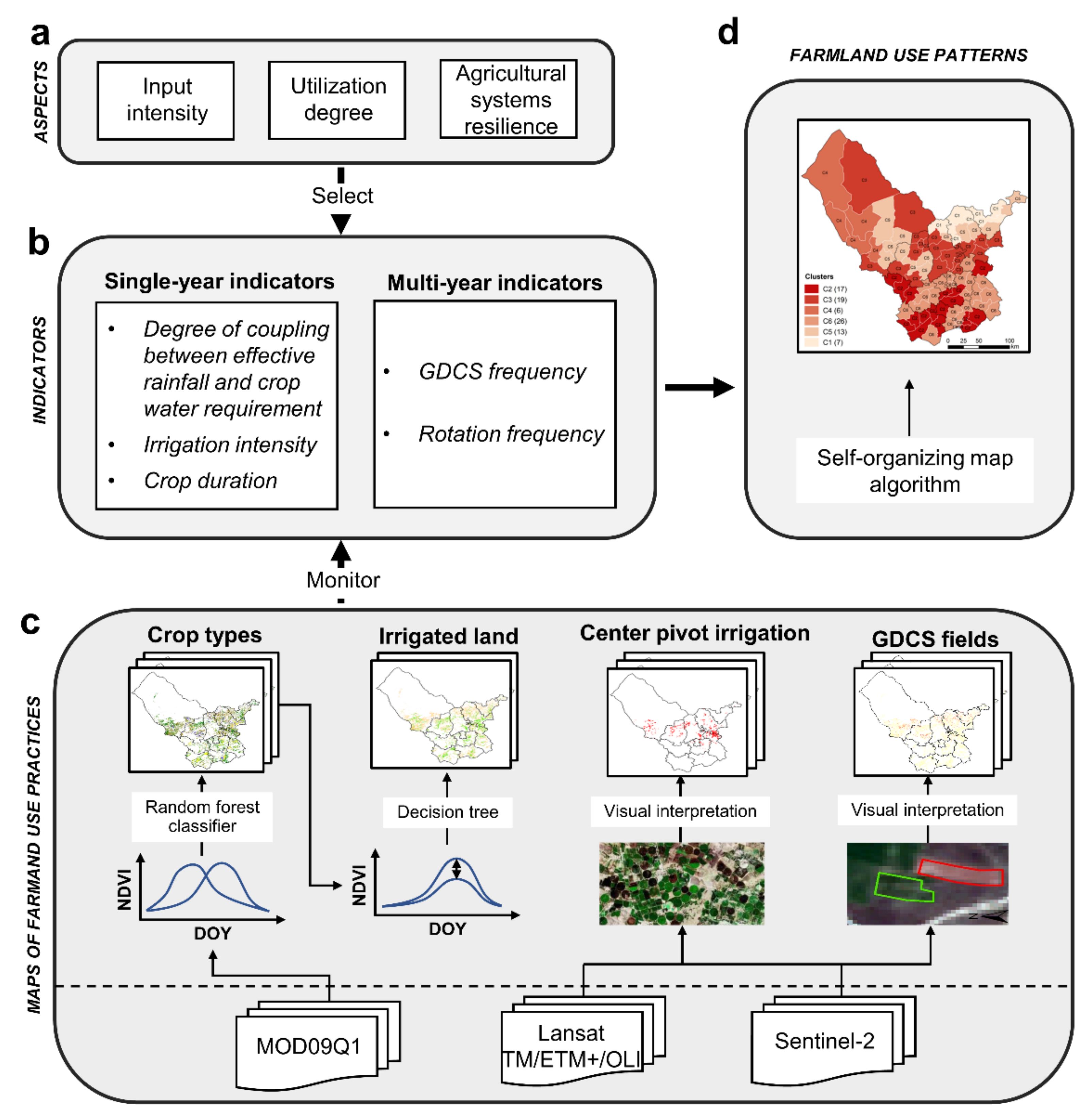
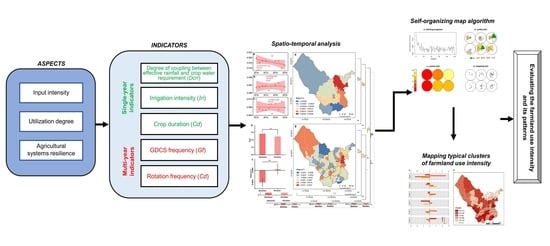
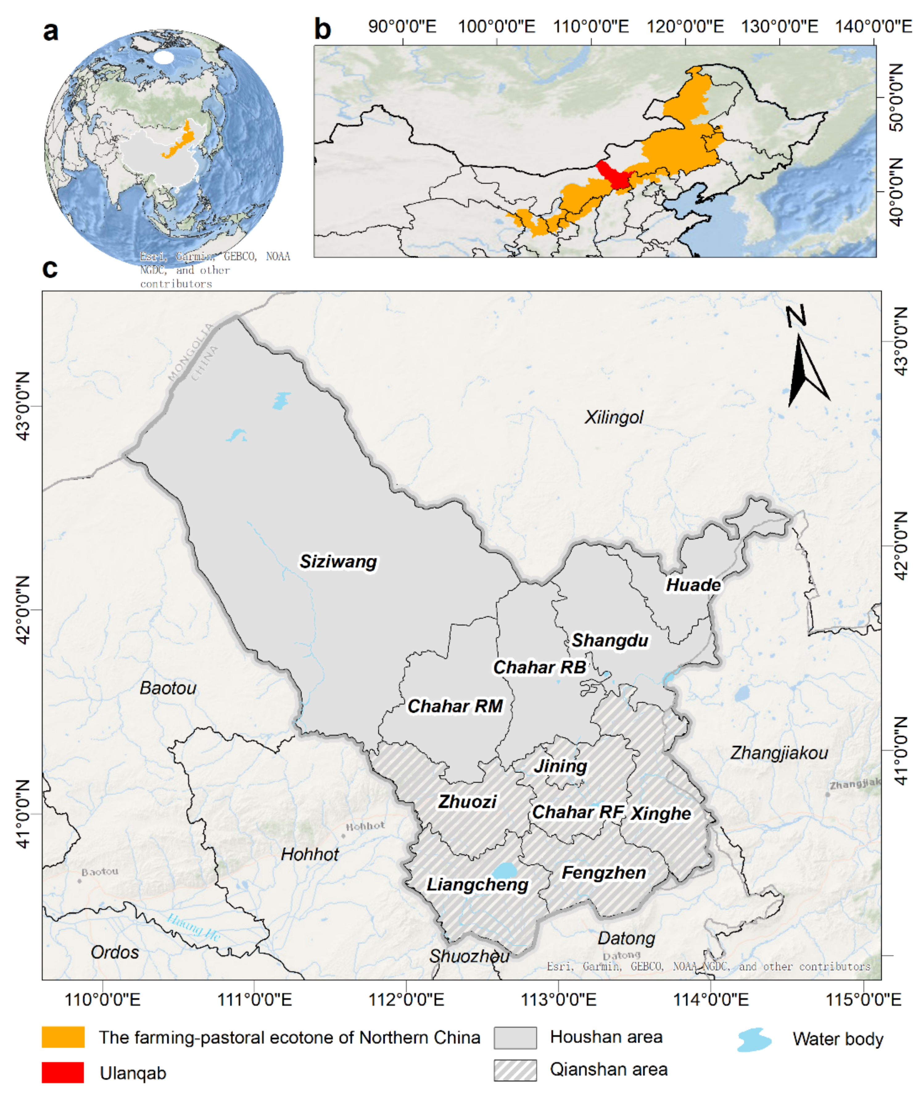
In this study, we first establish an assessment index system that fully considers the multiple aspects of farmland use intensity, including input intensity, utilization degree, and agricultural systems resilience. Second, taking the Ulanqab region in FPENC as an example and using remote sensing data as the main source, we produce maps of crop types, center pivot irrigation (CPI), and irrigated land from 2010 to 2019 by employing the methods proposed in our previous studies [46,47]. Third, we produce maps of the five farmland use intensity indicators and reveal their spatio-temporal dynamics during the study period. Finally, we apply SOM to recognize similar patterns in farmland use intensity.

2. Materials and Methods

2.1. Study Area

As shown in Figure 1, Ulanqab lies in the middle of the farming–pastoral ecotone of Northern China, with latitude and longitude spanning from 39°37′–43°28′N, 109°16′–114°49′E. Ulanqab includes eleven banners and counties, namely Fengzhen, Zhuozi, Xinghe, Liangcheng, Jining, Chahar Right Front Banner, Siziwang Banner, Shangdu, Huade, Chahar Right Back Banner, and Chahar Right Middle Banner, and comprises an area of nearly 5.47 × 10⁴ km2. Dominated by a semi-arid temperate continental monsoon climate characterized by cold dry winters and warm wet summers, this area receives a mean annual total precipitation of 150 to 450 mm, with more than 70% of the rainfall occurring in August and September [48]. The mean annual temperature of the district ranges from 0 to 18 °C, and the frost-free period varies from more than 140 days in the south to less than 100 days in non-agricultural areas of Siziwang. The Daqing Mountains separate Ulanqab into two parts, with the Qianshan area in the south and the Houshan area in the north, which introduces huge differences in agroclimatology between these two areas. Farmers in Ulanqab mainly grow potato, spring wheat, maize, sunflower, and naked oats, and their planting area reaches approximately 75% of the total planting area [46].

2.2. Data and Processing

2.2.1. Satellite Imagery

For mapping GDCS fields and center pivot irrigation, Landsat TM/ETM+/OLI and Sentinel-2 imagery were downloaded for the time period of 2010 to 2019 from the United States Geological Survey (USGS; https://glovis.usgs.gov/, accessed on 15 July 2020). MODIS/Terra Surface Reflectance 8-Day L3 Global 250m (MOD09Q1) from April to October for 2010–2019 was used for crop classification. Then, the MODIS Reprojection Tool was used to mosaic and reproject the obtained MOD09Q1 tiles. In addition, based on the MODIS data, the Normalized Difference Vegetation Index (NDVI) was derived according to the equation given by Braun and Herold (2004) [49]. Finally, the Savitzky-Golay (SG) filter provided in the Timesat 3.3 software package (Lund University, Lund, Sweden) was applied for noise reduction of the NDVI time-series data.

2.2.2. Meteorological Records

In this paper, daily meteorological variables, including precipitation, wind speed at 2 m height, air temperature at 2 m height, net radiation at the crop surface, soil heat flux density, saturation vapor pressure, actual vapor pressure, psychrometric constant, and slope vapor pressure curve, were acquired to calculate the effective rainfall and crop water requirement. The above in situ meteorological records across Ulanqab from 2000 to 2019 were collected from three available meteorological stations: the Huade station, Siziwang station, and Jining station. These data were downloaded from the China Meteorological Data Sharing Service Systems (http://data.cma.cn/, accessed on 1 September 2020).

2.2.3. Crop Phenology Data

Phenological data offer an effective way to measure the number of days required by crops to mature from sowing to harvesting, namely the crop duration. In this paper phenological data were obtained through two methods: (i) an in situ observation method and (ii) a questionnaire survey. The in situ phenological records of Ulanqab were provided from 1991 to 2013 by the China Meteorological Data Sharing Service System (http://data.cma.cn/, accessed on 21 March 2020). These data contain the station name, crop type, growth stage, and date. Furthermore, we calculated the average sowing and harvesting date based on the time-series historical records [46]. However, the in situ phenological records of sunflower in the Qianshan area and maize in the Houshan area are absent. Therefore, we conducted a questionnaire survey from mid-July to late-August in 2018 to ask the farmers about the timing of sowing and harvesting events of the two missing crops. After removing survey responses with incomplete information, 304 valid questionnaires remained for further data analysis.

2.2.4. Ancillary Data

Annual statistical yearbooks of Ulanqab were used to evaluate the accuracy of crop classification. These yearbooks provide detailed crop acreage data at a county level from 2010 to 2019. We evaluated the accuracy of the irrigation maps by incorporating ancillary information, such as the second national land survey county-level database of Ulanqab, Landsat images, and Google Earth imagery. Furthermore, we collected irrigation volumes of different crops under different irrigation techniques from the industrial water use quota information of Inner Mongolia in 2020 [50]. Our previous study conducted crop mapping and irrigated area mapping in Ulanqab from 2015–2019, and these existing results are also used in this study [46].

2.3. Methods

2.3.1. Mapping Methods of Crop Types, GDCS Fields, Irrigated Land, and CPI

The methods proposed in our previous studies [46,47] were used to map crop types, GDCS fields, irrigated land, and center pivot irrigation.
The NDVI profiles of different crops types can vary greatly during the growing season. We constructed NDVI profiles using ground truth crop samples and crop phenology data, and the results indicate the NDVI values of cereal crops, potato, maize, and sunflower peak at the day of year (DOY) 193, DOY 217, DOY 217 (or DOY 225), and DOY 217 (or DOY 225), respectively. Besides, the NDVI values of maize grow at a faster rate than those of potato and sunflower before DOY 217. Compared to potato and maize, the NDVI values of sunflower remained at a high level after DOY 217 (or DOY 225) [46]. Given these differences, we selected training samples for these main crops and then employed a random forest classifier to obtain the annual crop maps in Ulanqab from 2010–2019 (Figure 2c). Then, the irrigated and rainfed crop samples were collected from Landsat images and Google Earth imagery.
In this study, irrigated land mapping is based on the identification of irrigated crops and rainfed crops. Our previous study suggested that the peak NDVI of the irrigated crop is significantly higher than that of the rainfed crop [46]. Thus, we estimated the NDVI thresholds (Table A1) and then applied a decision tree to distinguish irrigated crops from rainfed crops. Taking maize of the Houshan area in 2012 as an example, all values less than or equal to 0.661 were considered rainfed whereas all values greater than 0.661 were considered irrigated. Finally, we obtained the irrigation map of Ulanqab by merging the irrigated crops (Figure 2c).
According to the questionnaire survey and the crop calendar, farmers usually plowed the inactive GDCS fields for the first time in mid-July, while the crops start to be harvested from early September. Namely, during late July and late August, GDCS fields remain unvegetated, while other fields are covered with vegetation. Hence, based on the differences in optical properties, the GDCS fields were distinguished from the other fields by performing a visual interpretation (Figure 2c).
Center pivot irrigation (CPI) is a system of crop irrigation in which equipment revolves around a central pivot point resulting in a circular pattern when viewed from the sky [47]. Because of the circular patterns, they can be detected through the visual interpretation of remote sensing imagery. As for the accuracy assessment of the above observations, two methods, namely a confusion matrix analysis [51] and a goodness-of-fit measure [52] were used in this study.

2.3.2. Single-Year Indicators of Farmland Use Intensity (SIFIs)

(1)
Degree of coupling between effective rainfall and crop water requirement
The degree of coupling between the effective rainfall and the crop water requirement (Dcrr) refers to a ratio between the two during the growth period of crops. The formula for Dcrr is as follows:
Dcrr = Pe/ETc
where Pe is the effective rainfall, which represents useful or utilizable rainfall for crop production for each growth period. Here, Pe was estimated by employing a fixed percentage of rainfall method (see Equation (4)). ETc is the crop water requirement for each growth period. Here, higher Dcrr signifies lower farmland use intensity. Given that no crops are planted during the inactive period of the GDCS, the Dcrr of the GDCS fields is set to 1. When calculating the Dcrr in the whole growth period of each crop, Pe and ETc are the total effective rainfall and the total crop water requirement for the whole growth period, respectively. A single crop coefficient approach is employed to estimate the ETc, which is formulated as follows:
ETc = Kc × ET0
where Kc is the crop coefficient; ET0 is the reference crop evapotranspiration, which is computed with the Penman-Monteith equation [53]. The formulae for the FAO-PM is as follows:
E T 0 = 0.408 R n G + r 900 / T + 273 u 2 e s e a / + r 1 + 0.34 u 2
where is the slope vapor pressure curve; Rn is the net radiation at the crop surface; G is the soil heat flux density; r is the psychrometric constant; u2 is the wind speed at 2 m height; T is the air temperature at 2 m height; es, ea, and esea are saturation vapor pressure, actual vapor pressure and saturation vapor pressure deficit, respectively.
Kc is determined by the single (time-averaged) crop coefficient approach recommended by FAO-56 [53]. Kc at the mid-season stage (Kcmid) and Kc at the end of the late-season stage (Kcend) were acquired according to the guideline (Table A2). However, Kcini is subject to the effects of large variations in wetting frequencies and, therefore, refinements to the value used for Kcini should always be made. Considering the lack of parameters for refinements, we introduced the Kcini of main crops from relevant studies conducted in or near Ulanqab.
Given the availability and applicability of the data, we measured Pe, employing a fixed percentage of rainfall method, which is simplified by the following equation [54,55]:
Pe = a × P
where P is the total rainfall over a certain period; a is a fixed percentage to be given by the user to account for losses from runoff and deep percolation, typically ranging from 0.7 to 0.9. Considering there is little surface runoff and deep percolation in the traditional dry farming area of Northern China, we here set a to a value of 0.9.
(2)
Irrigation intensity
In this paper, we refer to irrigation intensity as the irrigation volumes of different crops under different irrigation techniques. The formula for irrigation intensity (Iri) is as follows:
Iri = gij
where gij is the irrigation volume of the ith crop under the jth technique.
In Ulanqab, flood irrigation, an ancient method, is widely adopted by small farmers, whereas advanced irrigation systems, including center pivot, sprinklers, and drip irrigation are prevalently used by large farmers. However, compared with center pivot irrigation, sprinklers and drip irrigation comprise a small proportion in this area, and it is difficult to discriminate these two irrigation methods through remote sensing imagery. Therefore, we only compared the irrigation quotas of flood irrigation and center pivot irrigation for main crops, which were collected from the industrial water use quota of Inner Mongolia in 2020 (Table A3).
(3)
Crop duration
Crop duration refers to the number of days required by crops from sowing to harvesting. The formula for crop duration (Cd) is as follows:
Cd = DOYtDOY0
where DOY0 and DOYt are sowing date and harvesting date in day-of-year (DOY), respectively. The sowing and harvesting date for crops of the Qianshan and Houshan areas were collectively obtained from the long-term in situ phenological records and questionnaire (Table A4).

2.3.3. Multi-Year Indicators of Farmland Use Intensity (MIFIs)

(1)
GDCS frequency
GDCS frequency refers to the ratio of the number of years during which the fields experience GDCS practice, namely the inactive phase, to the number of years spanned by a time interval. The GDCS farmers generally leave GDCS fields inactive within two to five years [46], thus farming practices during a time interval of five years are enough to reveal the periodical farmland use intensity. Accordingly, we calculated GDCS frequency (Gf) according to the following formula:
Gf = tf/T
where Gf is GDCS frequency, ranging from 0 to 1; tf is the amount of times that GDCS fields are inactive within a time span of five years; T is the time interval (i.e., 5).
(2)
Rotation frequency
Rotation frequency refers to the ratio of the number of years during which the fields experience crop rotation practice to the number of years spanned by a time interval. Rotation frequency (Rf) can be calculated as follows:
Rf = tf/T
where Rf is rotation frequency, ranging from 0 to 1; tf is the number of years during which the fields experience rotation practice; T is the time interval (i.e., 5).

2.3.4. Self-Organizing Map Algorithm

The above five indicators highlight different high-value areas. As such, estimation of farmland use intensity is a multidimensional issue that relates to a range of individual processes and therefore cannot be fully represented by only one metric subject [56]. The self-organizing map, an effective clustering method [57,58], has been widely adopted in visualizing and interpreting linear and nonlinear relationships in multi-dimensional data for classification purposes [59]. As a result, we attempted to recognize similar patterns of farmland use intensity using a SOM. More details of a SOM are described by Wehrens and Kruisselbrink (2018) [58]. In this paper, all SOM calculations were performed with the RStudio software with the free Kohonen package available at https://github.com/cran/kohonen/blob/master/NEWS (accessed on 21 February 2021). Considering the number of indicators, we chose a SOM with a neuron structure of 3 × 2 to explain the various patterns of farmland use intensity that can occur across Ulanqab.

3. Results

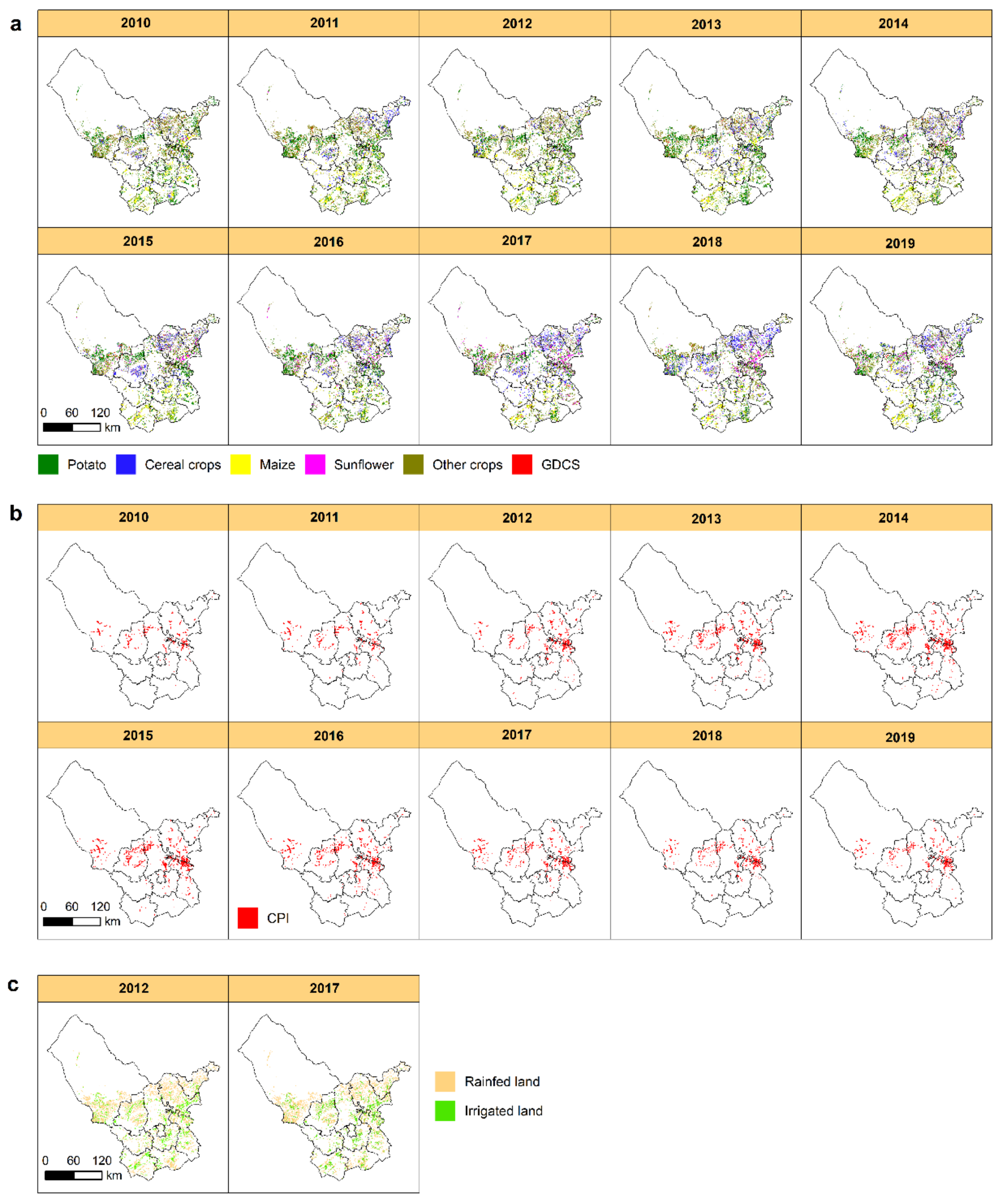
3.1. Detection of the Crop Types, CPI, and Irrigated Lands in Ulanqab from 2010–2019

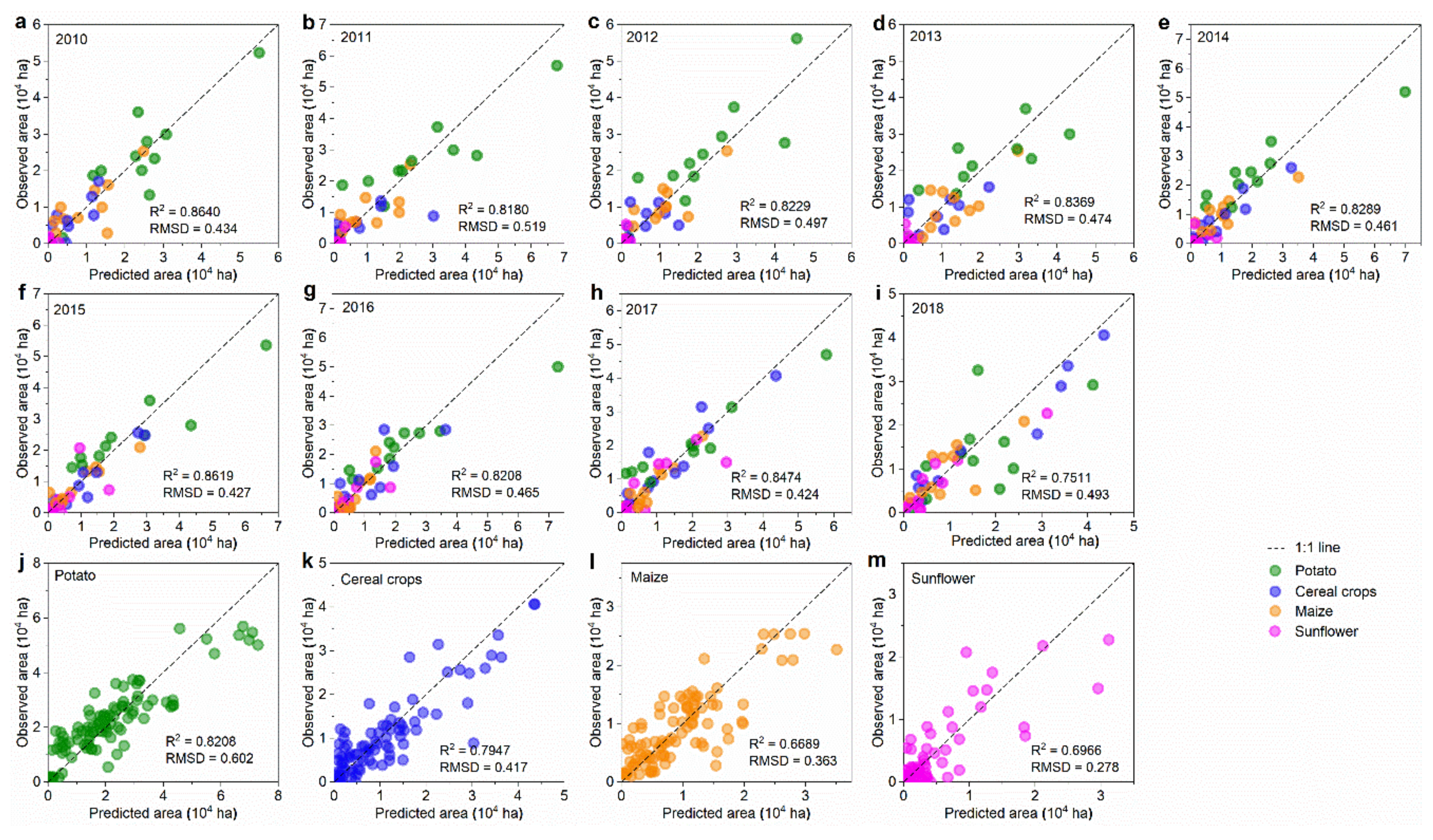
We obtained maps of the crop types, CPI, and irrigated land in Ulanqab from 2010 to 2019 (Figure 3) by employing the method mentioned. The scatter plots of the county-level crop acreage observations versus predictions for 2010–2018 suggest that the R2 values ranged from 0.75 to 0.86, and the root-mean-square deviation (RMSD) values ranged from 0.42 to 0.52 (Figure 4a–i). The classification results for 2019 suggested an overall classification accuracy of 78.1% (Table A5). In addition, the accuracy evaluation results by crops (Figure 4j–m) show that the R2 values of potato, cereal crops, maize and sunflower were 0.82, 0.80, 0.67, and 0.70, respectively, suggesting a generally good fit. The confusion matrix analysis of irrigated land mapping also exhibits a reasonable accuracy, with overall classification accuracies of 84.55% and 90.17% (Table 1), and Kappa coefficients of 0.69 and 0.79 for 2012 and 2017, respectively.

3.2. Evaluation of SIFIs from 2010–2019

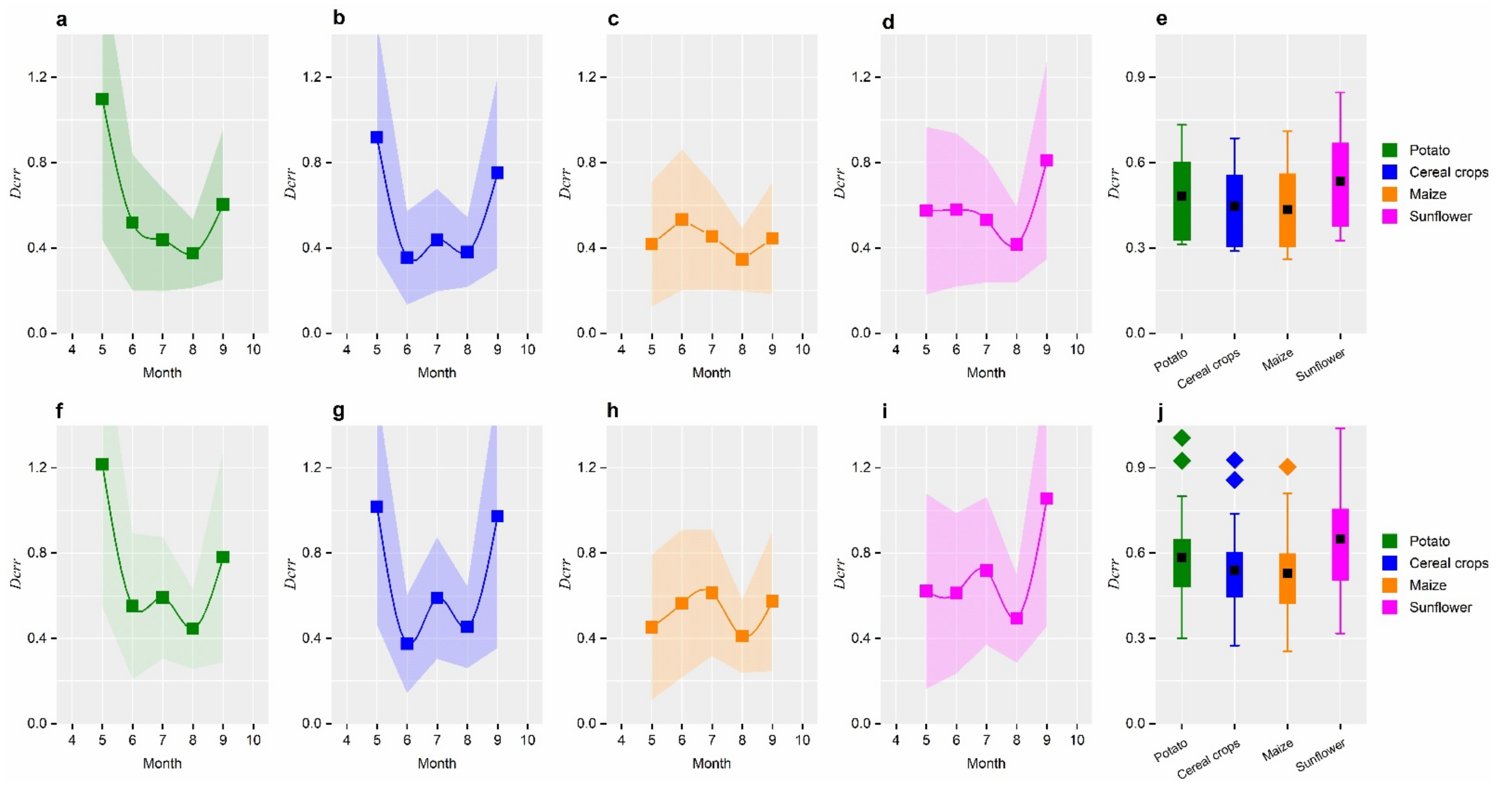
3.2.1. Spatio-temporal Dynamics of Dcrr in Ulanqab from 2010–2019

(1)
Estimation of Dcrr for main crops
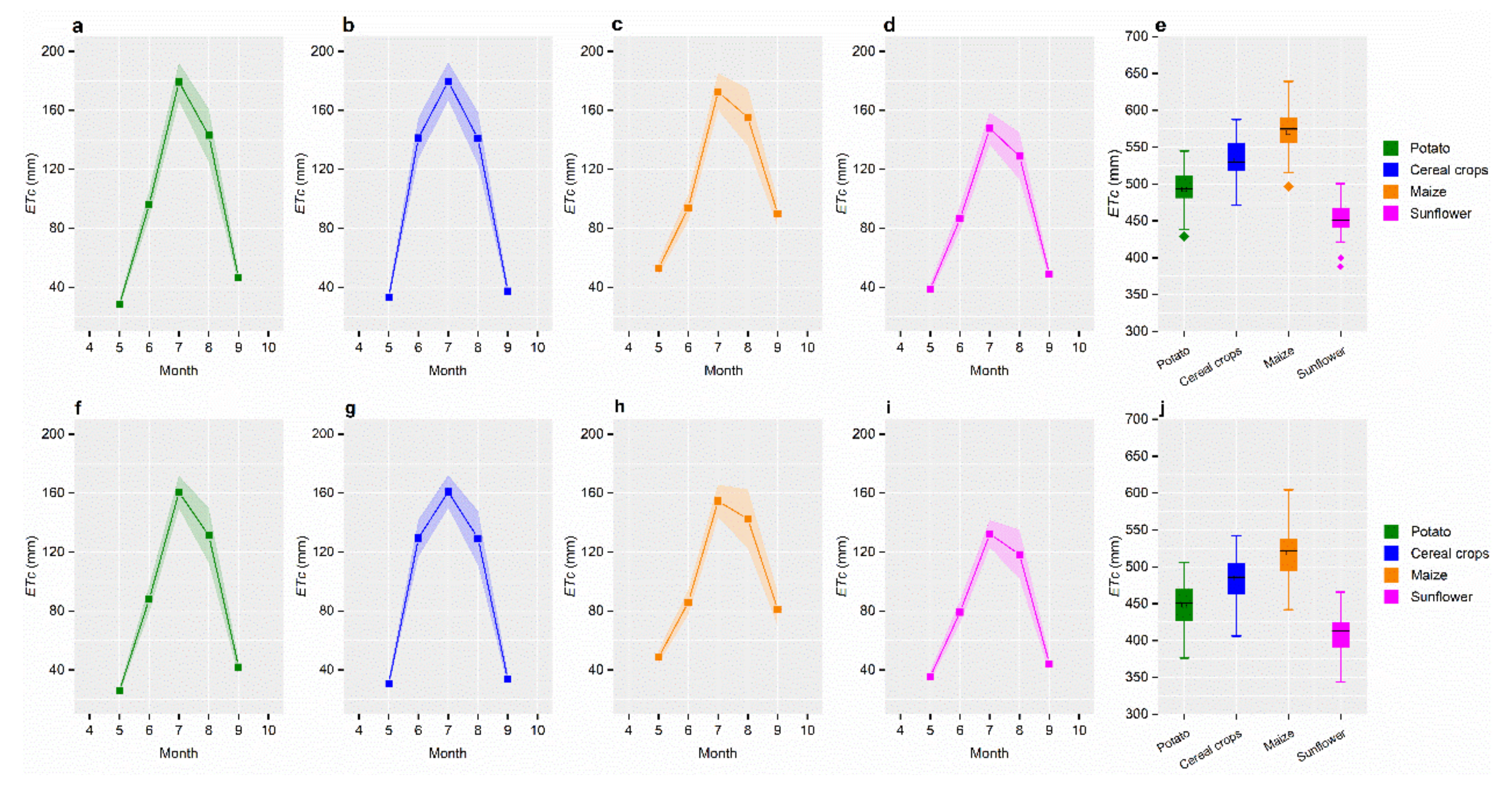
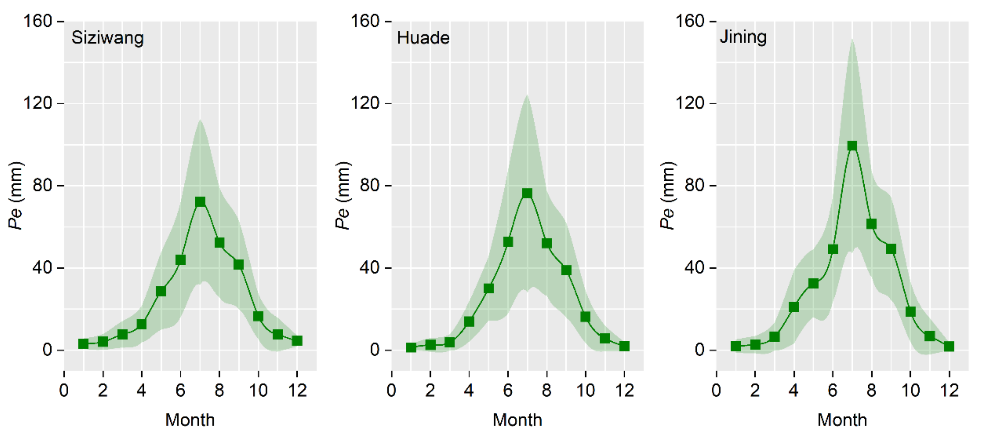
Due to space limitations, we do not present here the estimation results of ETc and Pe (see Appendix A for details, Figure A1 and Figure A2). The monthly degree of coupling between the effective rainfall and the crop water requirement (mDcrr) and Dcrr during the whole growing season (tDcrr) of main crops showed that, in Ulanqab, the highest tDcrr was observed for sunflower, followed by potato, wheat, and maize (Figure 5). Furthermore, the tDcrr in the Qianshan area is about 20% higher than that in the Houshan area. The mDcrr analysis shows that in June, wheat was the crop with the lowest mDcrr because wheat was at the tillering stage and needed more water than other crops during this period, while the precipitation was less at this time; in July, wheat at jointing and heading stages required the largest ETc, and then the Pe in Ulanqab reached its highest level, and therefore an increasing trend of mDcrr was observed.The mDcrr curve of potato is similar to that of wheat and is thus not discussed. The mDcrr of maize was relatively low. The mean value mDcrr of sunflower was higher than that of other crops owning to synchronous rainfall and less ETc.
(2)
Analysis of spatio-temporal patterns of Dcrr
Subsequently, based on the crop type map and the estimations of Dcrr for crops, we generated pixel-wise Dcrr maps of Ulanqab for 2010–2019. To intuitively present the spatio-temporal heterogeneity, we carried out statistics of Dcrr at different administrative scales and analyzed their change trends during this period. In general, over the past ten years, the Dcrr of Ulanqab experienced a statistically insignificant decline (R2 = 0.22, p = 0.17) (Figure 6g). However, the value and change trend of Dcrr vary considerably temporally and spatially. Of the counties, Xinghe had the highest Dcrr of 0.58 in 2019, while Chahar RM (0.49), Siziwang (0.49), and Chahar RB (0.49) had a lower Dcrr. Furthermore, the Dcrrs of Shangdu and Xinghe decreased significantly (Figure 6d), which was related to the potato shrinkage and the wheat expansion in these two counties. A town-level analysis suggested that 36.36% of the towns showed an upward trend in Dcrr, and these towns are mainly located at the junction area between Xinghe and Shangdu, and the northwest pastoral area of Siziwang. Conversely, 63.64% of the towns showed a downward trend in Dcrr, which was due to the increase in the planting area of wheat and maize in these towns. Results of one-way ANOVA, with pairwise comparisons using the Tukey test (Figure 6e), show that Dcrr in the Qianshan area was significantly higher than that in the Houshan area. In addition, the Dcrr in the Qianshan and the Houshan areas in 2010–2019 witnessed insignificant downward and insignificant upward trend, respectively (Figure 6f).
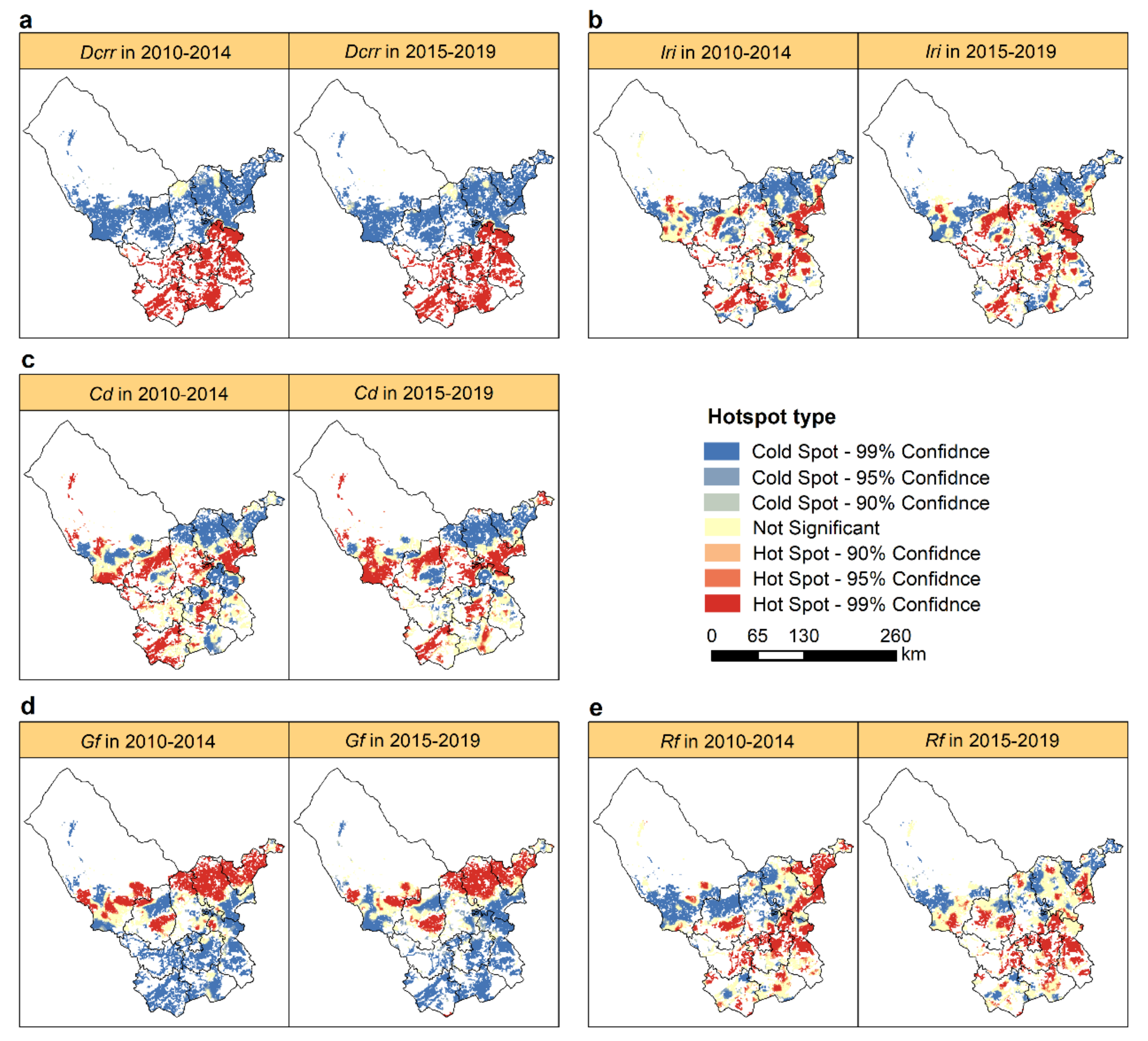
To measure the degree of spatial clustering of Dcrr, we performed a hotspot analysis of a 1km square grid using the optimized hotspot analysis tool of Esri ArcGIS 10.2 (Figure 7a). The results show that high-value grids are mainly concentrated in the Qianshan area. This is due to the following two reasons: there is more Pe in the Qianshan area (Figure A2); according to the crop classification results, wheat planting is considerably more frequent in the Houshan area than that in the Qianshan area.

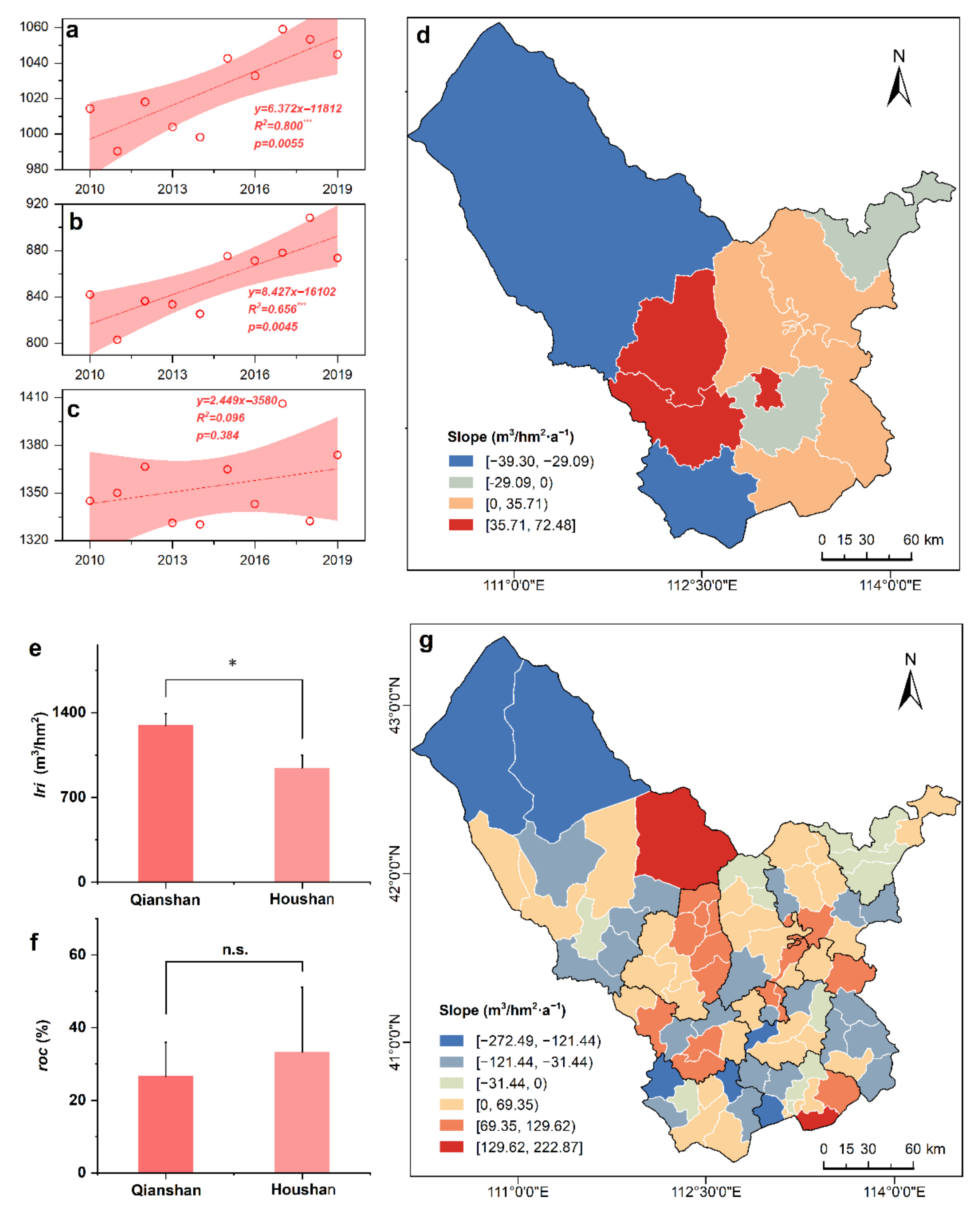
3.2.2. Spatio-temporal Dynamics of Iri in Ulanqab from 2010–2019

The irrigation intensity (Iri) trend analysis highlights a statistically significant increase (R2 = 0.80, p < 0.01) in Iri of Ulanqab in the past ten years, rising from 1014 m3/hm2 in 2010 to 1045 m3/hm2 in 2019 (Figure 8a). The county-level comparison shows that in 2019, Iris of Zhuozi, Chahar RF, and Liangcheng were in the top three ranks. It was moreover found that Iris of Liangcheng, Chahar RF, Siziwang, and Huade decreased, which was closely related to the introduction of a policy to transfer irrigated lands into rainfed lands. Our results report a large spatial heterogeneity in Iri at the town level (Figure 8g), indicating that 56.82% of towns experienced an increase in Iris, mainly for the CPI expansion, while 43.18% of the towns around the Daihai lake experienced a decrease in the Iris. Although Iri in the Qianshan area is significantly higher than that in the Houshan area (Figure 8e), the gap is narrowing (Figure 8f).
The high-value areas of Iri in Ulanqab are mainly distributed in the bordering area between Xinghe and Shangdu, the bordering area between Chahar RM and Chahar RB, the area around Daihai lake and Huangqihai lake, and the Tabu River basin of Siziwang (Figure 7b). The average annual proportion of Iri hotspots at a 99% confident level increased from 25.54% in 2010–2014 to 27.96% in 2015–2019 (Table A6). The newly emerging hotspot area of Iri was mainly distributed in the northern Chahar RM and the junction area between Xinghe and Shangdu, whereas the hotspot areas of Iri mostly disappear around the Daihai lake due to the implementation of agricultural water conservation. For example, 667 wells were abandoned in Liangcheng from 2016 to 2018 to reduce irrigation water usage [60].

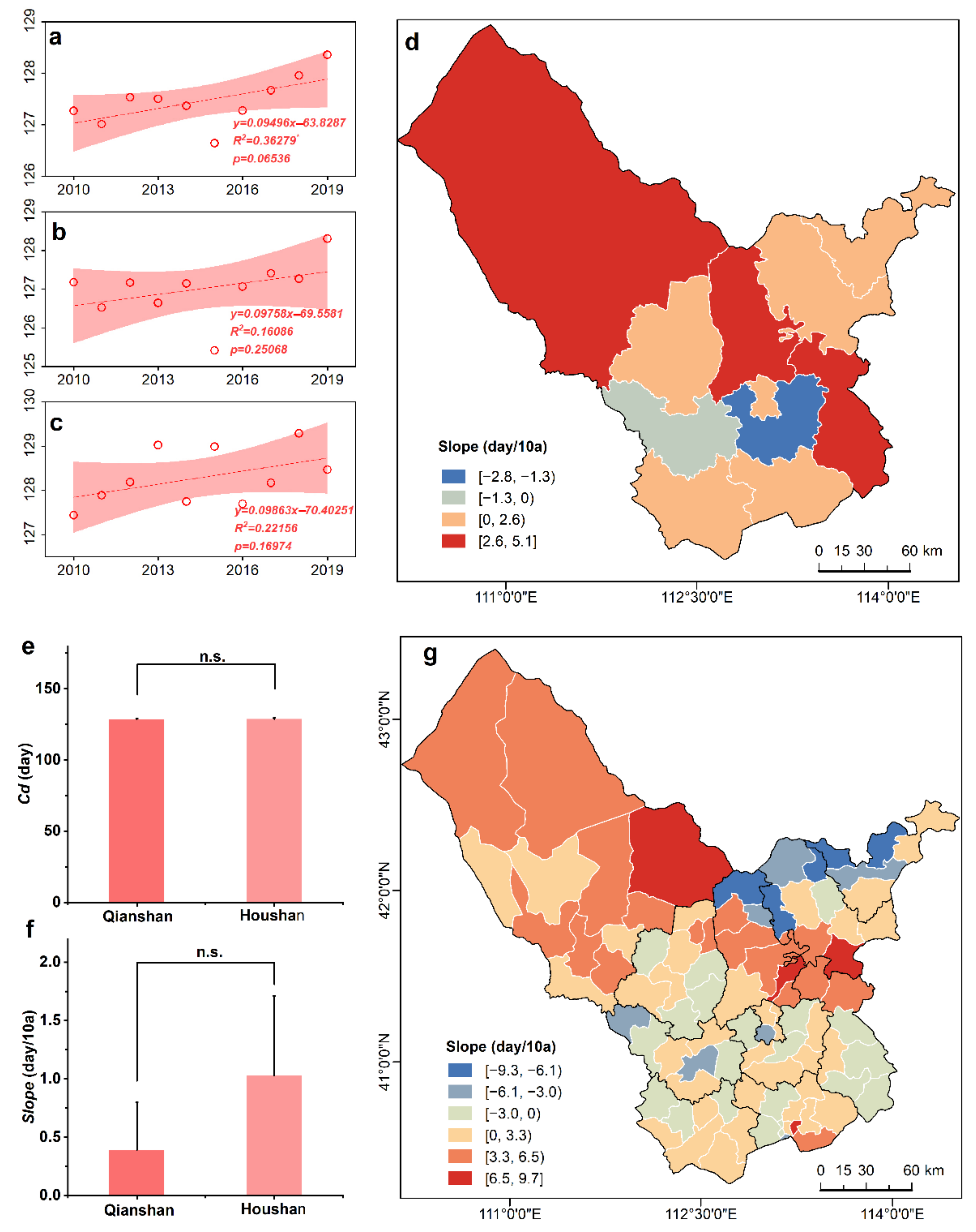
3.2.3. Spatio-Temporal Dynamics of Cd in Ulanqab from 2010–2019

Figure 9a shows that during these ten years, the crop duration (Cd) of Ulanqab had slightly lengthened from 127 to 128 days. Of the counties (Figure 9d), the Cds were longer in counties of the Houshan area with poorer heating and lower temperature. A town-level analysis suggested that 62.50% of the towns showed an upward trend in Cd, while 37.50% of towns showed a downward trend in Cd (Figure 9g). A regional-scale comparison showed that the Qianshan area owned an insignificantly longer Cd than the Houshan area (Figure 9e). Similarly, a significant difference was not observed between the slopes of the two groups (Figure 9f); the main reason may be socioeconomic rather than natural factors.
Figure 7c shows that the high-value grids of Cd in Ulanqab were more likely clustered around an irrigation area, which can guarantee the ETc of crops with long Cd. The average annual proportion of Cd hotspots increased from 35.14% in 2010–2014 to 41.62% in 2015–2019 at a 99% confidence level (Table A6). The newly emerged Cd hotspots were mainly detected in the southern agricultural area of Siziwang.

3.3. Evaluation of MIFIs from 2010–2019

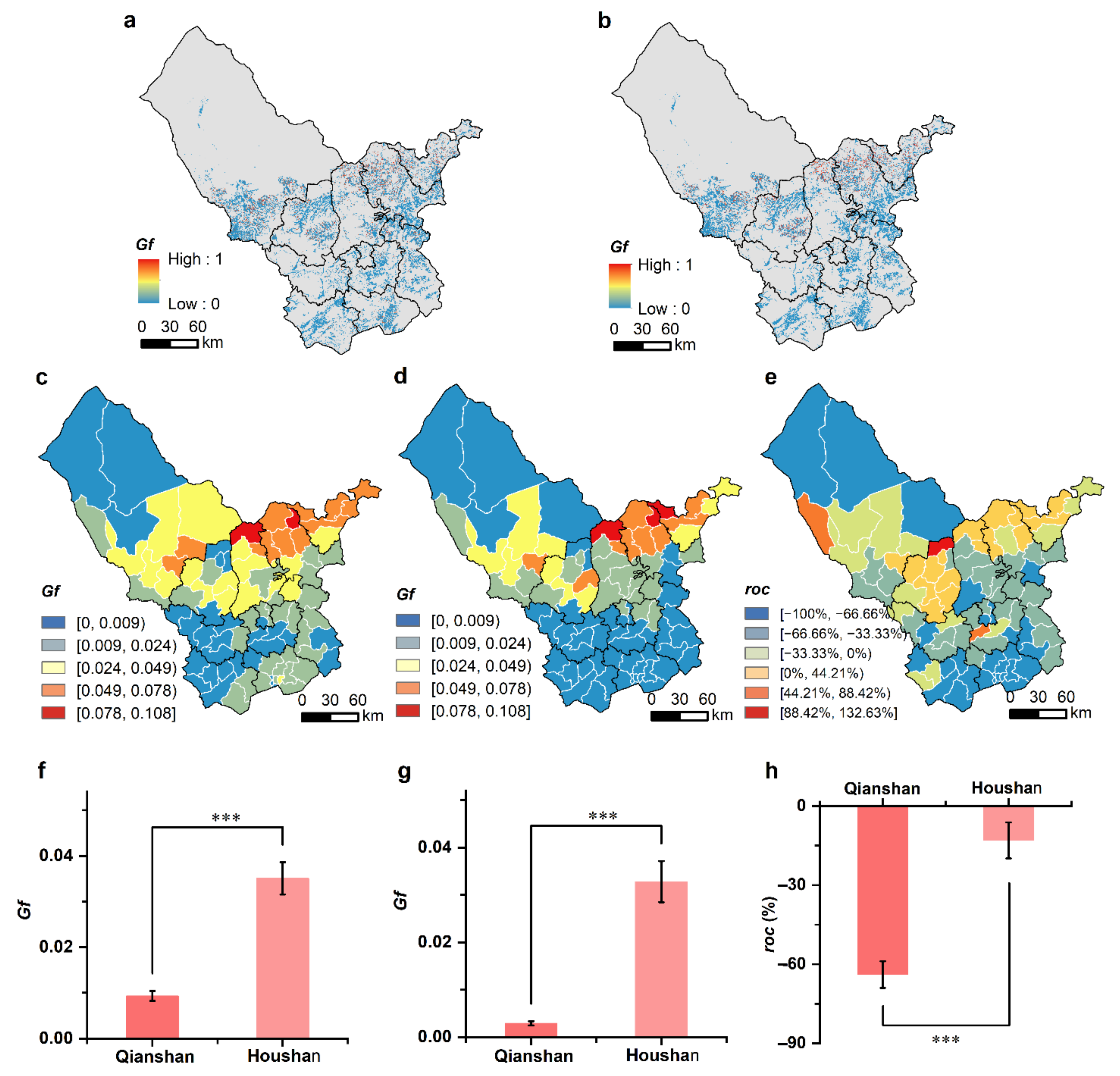
3.3.1. Spatio-Temporal Dynamics of Gf in Ulanqab from 2010–2019

Annual 30-m pixel size crop maps and raster calculator tool provided in Arcgis 10.2 were applied to obtain the pixel-wise GDCS frequency (Gf) maps in Ulanqab during two time intervals, namely 2010–2014 and 2015–2019 (Figure 10a,b). There was a clear downward trend in Gf, declining from 0.029 in 2010–2014 to 0.025 in 2015–2019. Furthermore, Figure 10f–h shows that the Gf in the Qianshan area was significantly lower than that in the Houshan area, and the Qianshan area (−63.87%) experienced a higher decline in Gf than the Houshan area (−13.02%). County-level results show (with the exception of an increase in the Gf of Chahar RM of 21.06%) that the Gfs in other counties show downward trends. Among them, Fengzhen, Liangcheng, and Xinghe had the larger decline, with a decrease of 88.30%, 77.71%, and 64.38%, respectively. Of the towns (Figure 10c–e), 77.27% showed a downward trend, whereas 22.73% of the townships, which are mainly located in the Northern Houshan area, increased the Gf.
Table A6 shows that the proportion of Gf hotspots decreased from 32.69% in 2010–2014 to 29.71% in 2015–2019, proving once again that farmers were increasingly inclined to adopt successive planting.

3.3.2. Spatio-Temporal Dynamics of Rf in Ulanqab from 2010–2019

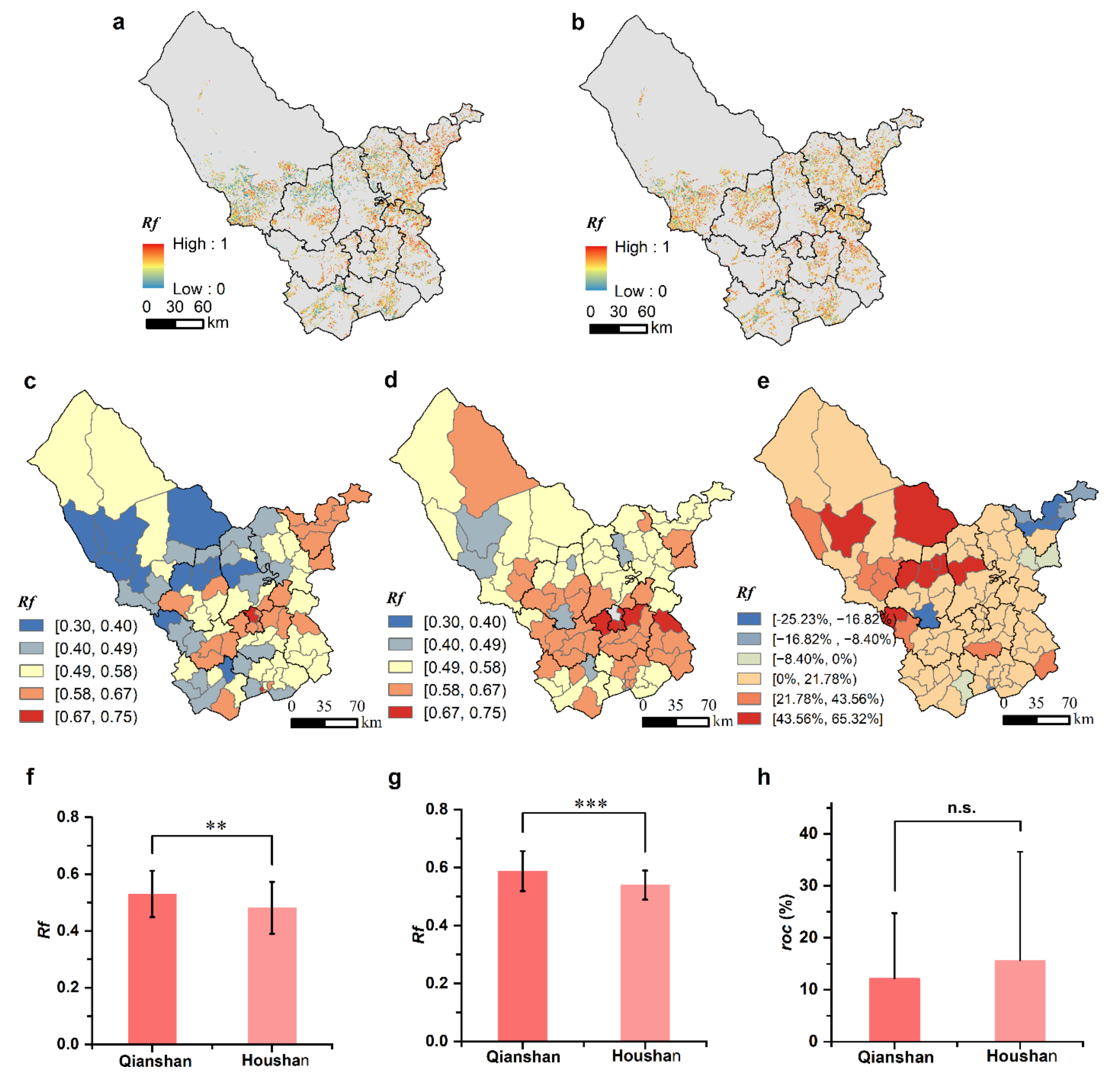
Pixel-scale rotation frequency (Rf) maps of Ulanqab in 2010–2019 were created using Equation (8) (Figure 11a,b). The results indicate that the Rf of Ulanqab increased from 0.49 in 2010–2014 to 0.55 in 2015–2019. The one-way ANOVA results (Figure 11f,g) indicate that Rfs of the Qianshan group were significantly higher than those of the Houshan group. Furthermore, the Rfs of the two groups show a general upward trend, and the growth rate of the Houshan group (12.55%) was higher than that in the Qianshan group (10.60%). A county-level comparison showed that, except for Huade, the Rfs of other counties had increased, and Chahar RM and Siziwang had also increased by more than 20%. Furthermore, our town level results (Figure 11c–e) also reported that 88.64% of the towns experienced an increase in Rfs, whereas 11.36% of the towns experienced a decrease in the Rfs. Hot spots of Rf increased in the towns of Western Chahar RM and the towns of Southern Siziwang (Table A6).

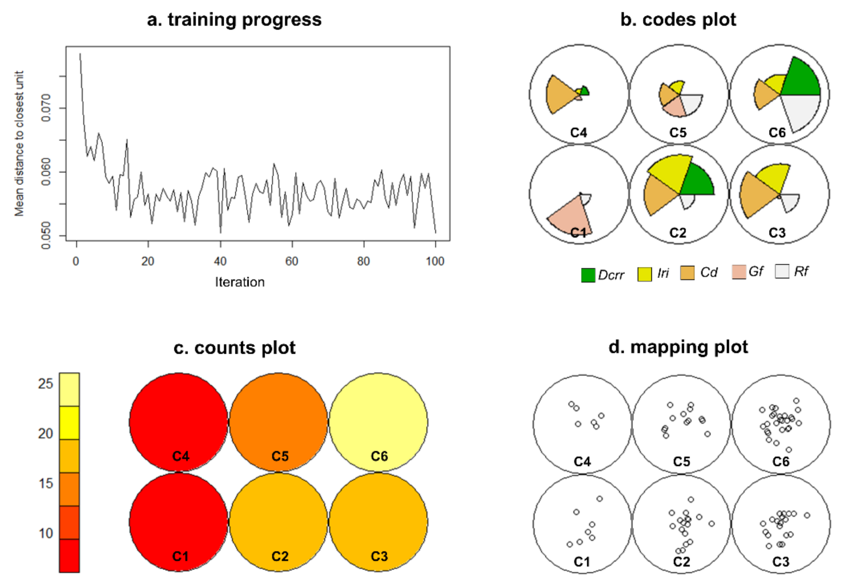
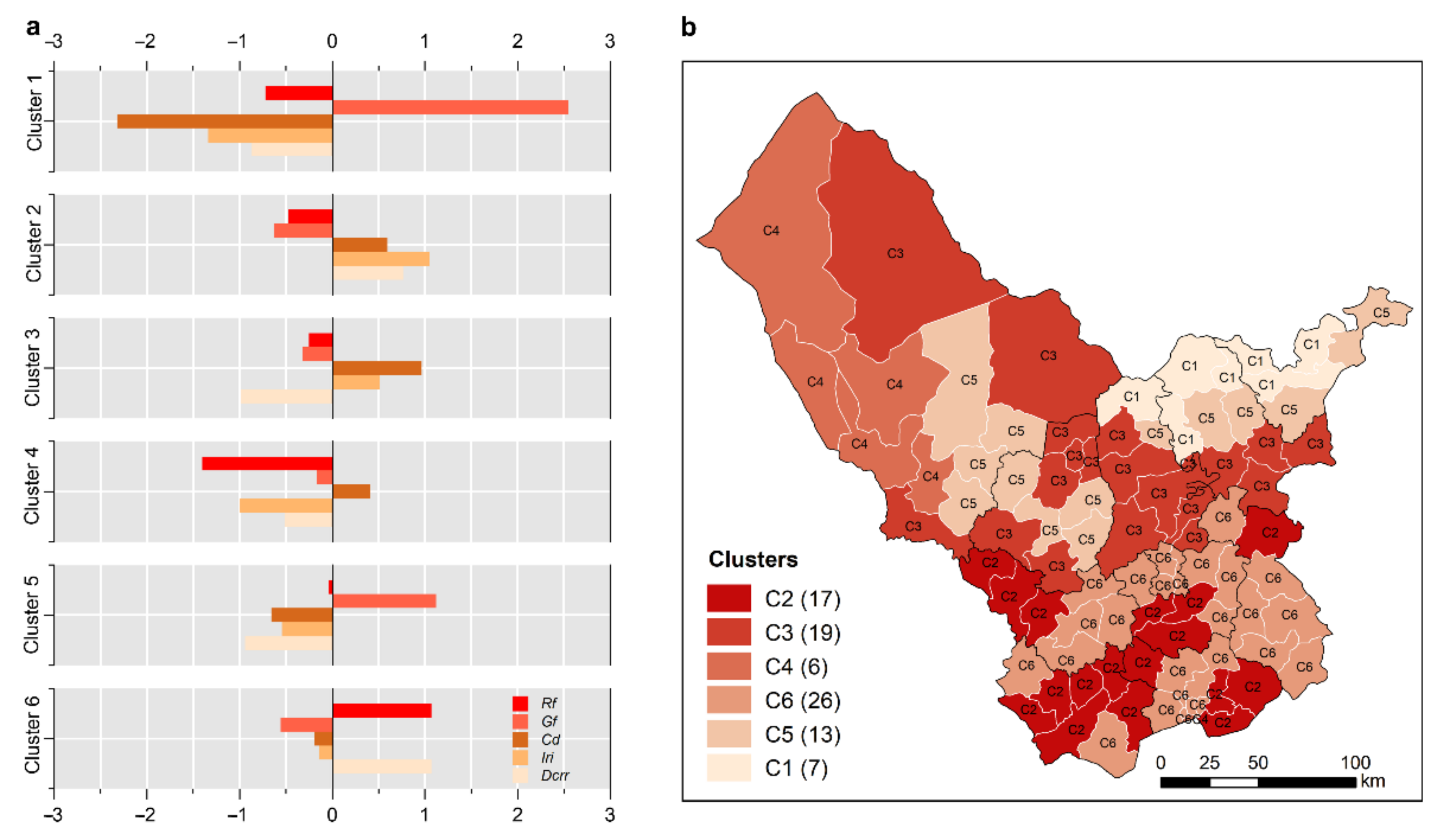
3.4. Mapping Typical Clusters of Farmland Use Intensity

The Kohonen package provided by R was used to train a SOM neural network for five farmland use intensity indicators at the town scale. The training progress is shown in Figure 12a, and finally, six similar farmland use intensity clusters are identified (Figure 12b). We also plotted a heat map of the node counts (Figure 12c) and a mapping plot (Figure 12d).
To describe the magnitude and direction of the different farmland use intensity indicators in each Cluster (C1–C6), we provided the deviation (±) from the mean z-score (=0) in Figure 13a. Positive and negative numbers thus signify above and below-average values respectively, whereas values close to zero represent that a specific indicator is close to the overall mean of the study area. The obtained six clusters are shown in Figure 13b.
Cluster 1, which occurred mainly in the Northern Houshan area, was characterized by low-intensive rain-fed cropping with a short Cd (−2.32), high Gf (+2.54), and low Iri (−1.34). Due to complex topography and sparse rainfall, farmers in Cluster 1 tended to have a higher willingness to adopt GDCS and grow drought-resistant crops such as wheat and naked oats.
Cluster 2 was related to high-intensive irrigated cropping with high Iri (+1.05), long Cd (+0.60), low Gf (−0.63), and high Dcrr (+0.76). This cluster contained 17 towns, mainly located in Southern Ulanqab along Daihai Lake and Huangqihai Lake. Thus, the ideal irrigation conditions provide a good foundation for planting long-duration crops. Despite that maize with high ETc was popularly grown in these areas, there was more precipitation in the Qianshan area, where a high Dcrr was observed.
Cluster 3 consists of 19 towns, mainly distributed in the Houshan areas. In regions where topographic conditions permit, local government and farmers prefer to introduce center pivot irrigation, sprinklers irrigation, and drip irrigation to grow potatoes. Notwithstanding the extensive distribution of irrigated fields, the irrigation intensity of Cluster 3 was lower than that of Cluster 2.
Similar to Cluster 1, the remaining three clusters also belong to the traditional dry farming area. The differences are as follows: there were dispersedly center-pivot irrigated fields in Cluster 4; Cluster 4, mainly occurring in Western Siziwang, contains six towns; as for Cluster 5, despite a similar cropping pattern with Cluster 1, it owns a higher farmland use intensity; Cluster 6, characterized by high Dcrr (+1.07) and high Rf (+1.07), occurs mainly in the Qianshan area; however, due to more favorable rainfall conditions, Cluster 6 owns higher Dcrr than other clusters.

4. Discussion

4.1. Implications

The changes in farmland use intensity over the past 10 years are mainly linked to national policies. In 2009, China launched the “National Plan for Increasing 50 Million Tons of Grain Production Capacity from 2009–2020”, and this plan pointed out that local governments in FPENC should expand irrigated areas, make more water-saving efforts, and improve the irrigation rate. With this background, advanced irrigation systems were introduced, and large areas of rainfed lands were converted to irrigated lands, ultimately leading to a rise in regional Iri. In addition, this plan also recommends a vigorous promotion of mulching technology in FPENC. Mulch provides favorable conditions for sunflower and maize, with high light and temperature requirements, prolonging the regional crop duration. China issued a document in 2016 asking for a crop rotation pilot in FPENC, which resulted in a significantly higher Rf in this region from 2015–2019, compared to 2010–2014. The decline in the Gf is mainly attributed to the tensing human–land relationship in addition to the significant increase in rainfall in the last decade, which has also reduced farmers’ willingness to adopt the GDCS practice.

4.2. Optimization of the Acreage for Main Crops

Table A3 suggests that potato has a relatively lower irrigation quota under different techniques. Moreover, the Ulanqab government makes efforts to build China’s potato capital and implement a potato staple-ization strategy. For the reasons above, local farmers should take potato as a superior crop and expand their potato acreage. Conversely, potato planted acreage in Ulanqab over the past decade has halved, dropping from 26.75 × 10⁴ hm2 in 2010 to 13.02 × 10⁴ hm2 in 2019 [61]. Besides, Ulanqab still has 2% of its farmland as irrigated cereal crops, but spring wheat has the highest irrigation quota of 5000 m3/hm2. Therefore, the planting of cereal crops on irrigated lands should be limited. Because rainfed cereal crops own a higher drought tolerance than other crops, their cultivation is recommended even if the yield can decrease under drought constraints. In addition, considering that cereal crops require substantial water in the early growing period, and soil moisture is high after the inactive period of the GDCS, we suggest that cereal crops are suitable as the subsequent crop [46]. Maize and sunflower are thermophilic crops with a long crop duration of about 140 days. As Ulanqab has an accumulated temperature of 1615–3033 °C and a short frost-free period (95–145 days) [46], stable yields of maize and sunflower are probably threatened by an early frost. Thus, farmers should reduce maize and sunflower cultivation, especially in the Houshan area.

4.3. Promotion of the Crop Rotation

We found that in 22.68% of the farmlands, the same crop was grown continuously for many years (Table A7). The reason can be attributed to the high economic benefits of certain crops, strong demand for fodder crops for raising livestock, and severe land scarcity. However, the risks of continuous cropping to sustainable agriculture have received considerable concerns [62]. Continuous cropping will deplete nutrients and water of the same soil layer, easily triggering soil drought and degradation. In addition, it can lead to an imbalance of soil microbial communities and encourage the prevalence of diseases. For example, orobanche coerulescens is a parasitic plant that has been reported to attack sunflowers fields of continuous cropping in Inner Mongolia, causing a 10–50% loss in yield [62,63]. Besides, continuous cropping obstacles are common with potato. Our study suggests that 2.04% and 11.73% of fields have practiced continuous cropping of sunflower and potato in Ulanqab from 2015–2019 (Table A7). To reduce the risk of diseases, it is important to choose suitable crops for crop rotation of sunflower and potato. Rotating deep-rooted crops with shallow-rooted ones can benefit the soil by recovering moisture and nutrients in addition to improving the soil structure [64]. Given this, we recommend cropping sequences such as cereal crops–potato, maize–potato, and cereal crops–sunflower as the crop rotations in Ulanqab.
Moreover, Huang et al. (1987) and Jiang (1989) emphasized that a reasonable annual proportion of fields practicing GDCS in FPENC should be 33.33% [65,66], but in 2019, only a small proportion (2.40%) of fields adopted the GDCS practice in Ulanqab. Thus, the government should introduce subsidies to stimulate farmers to take this practice [46], especially in the dry farming areas (e.g., clusters 1, 4, 5, and 6).

4.4. Management Improvement of Irrigated Land

Our statistics also show that the total area of irrigated land has experienced a rapid expansion, with the share rising from 26.55% to 29.55%. The conversion from rainfed farmland to irrigated farmland mainly occurred in Cluster 3, due to the introduction of CPI. However, irrigation expansion threatens the scarce water resources of the region. An example is Chahar Right MB in Cluster 3 which has experienced a significant agricultural transformation over the last two decades, resulting in a groundwater decline from −553 mm in 2005 to −701 mm in 2018 according to the in situ records. This unprecedented challenge has forced the local government to initiate policies to prevent the continuous decline in the groundwater table. The local government has required the elimination of CPI in the Chahannaoer basin [67] and the conversion from irrigated land to rainfed land in the Daihai lake basin [60]. Besides, the switch from a sprinkler or flood irrigation to drip irrigation is also recommendable to prevent and mitigate the decline of water resources.

5. Conclusions

In this study, we established an indicator system, which included three single-year indicators and two multi-year indicators, for evaluating farmland use intensity in Ulanqab. Long-term satellite imagery, meteorology records, crop phenology data, and other ancillary data were combined to obtain maps of crop types, the prevalence of the CPI, and irrigated land in Ulanqab, Inner Mongolia, China, in 2010–2019, and the classification results evidenced reasonable accuracies. Moreover, we revealed the spatio-temporal dynamics of the five single farmland use intensity indicators during the study period by depicting their pixel-wise maps. Significant increases in Iri, Cd, and Rf of Ulanqab from 2010 to 2019 were found, whereas insignificant decreases were observed in Dcrr and Gf. We confirmed that farmers in this area were progressively inclined to higher farmland use intensity. Moreover, there was obvious spatial heterogeneity in the change trends, with the Dcrr, Iri, Cd, and Rf in the Qianshan area being higher than those in the Houshan area, and the Gf in the Houshan area being higher than that in the Qianshan area. Finally, we recognized six similar patterns of farmland use intensity over Ulanqab by applying the SOM algorithm and discussed the optimizing direction for future farmland use in areas with different farmland use intensity patterns.

Author Contributions

Conceptualization, X.C. and P.A.; methodology, X.C.; software, X.C.; validation, G.Z. and Y.J.; formal analysis, X.C.; investigation, G.Z., Y.J., S.M., L.J., Y.Z. and H.Z.; resources, X.C. and Z.P.; data curation, X.C., G.Z. and R.J.; writing—original draft preparation, X.C.; writing—review and editing, K.L. and A.S.-A.; visualization, X.C.; supervision, P.A., Z.P. and L.Y.; funding acquisition, P.A., Z.P. and X.C. All authors have read and agreed to the published version of the manuscript.

Funding

This research was funded by the National Natural Science Foundation of China (grant number 41871086), the Key R&D Program of Inner Mongolia, China (grant number 2020ZD0005, 2019GG016), and China Scholarship Council (grant number 201906350154).

Institutional Review Board Statement

Not applicable.

Informed Consent Statement

Not applicable.

Acknowledgments

The authors would like to thank the reviewers and editors for their constructive comments. We thank Arturo Sanchez-Azofeifa and Kati Laakso for their linguistic assistance during the preparation of this manuscript.

Conflicts of Interest

The authors declare no conflict of interest.

Appendix A

Table A1. Thresholds in decision treens for distinguishing irrigated crops from rainfed crops in the Houshan and the Qianshan areas.
RegionsCropsThresholds in 2012Thresholds in 2017
Houshan areaPotato0.6770.687
Cereal crops0.5770.622
Maize0.6610.670
Sunflower0.7460.705
Qianshan areaPotato0.7320.741
Cereal crops0.5920.620
Maize0.6950.758
Sunflower0.7050.719
Table A2. Single (time-averaged) crop coefficients for main crops in Ulanqab.
CropsKciniKcmidKcend
Potato0.241.150.75
Spring wheat0.231.150.4
Maize0.451.20.35
Sunflower0.4510.35
Table A3. Irrigation quotas of main crops under different irrigation techniques in Ulanqab (m3/hm2). Considering the completeness of data, we collected the gij under 75% probability of irrigation.
Irrigation TechniquePotatoSpring WheatMaizeSunflower
Irrigated land Center pivot irrigation2970316027702090
Flood irrigation3310500043002790
Rainfed0000
Table A4. The sowing and harvesting dates, and crop duration for crops of the Qianshan and the Houshan areas.
RegionsMain CropsSowing DateDOY0Harvesting DateDOYtCrop Duration
Houshan areaPotato5.51269.10254128
Spring wheat4.301218.30243122
Naked oats5.11229.1245123
Maize5.512610.1275149
Sunflower5.101319.30274143
Qianshan areaPotato5.101319.15259128
Spring wheat5.101319.5249118
Naked oats5.251469.5249103
Maize5.101319.25269138
Sunflower5.2014110.8282141
Table A5. Accuracy measurements of crop classification for 2019.
PotatoCereal CropsMaizeSunflowerOther Crops
Producer’s accuracy (%)86.868.984.469.477.2
User’s accuracy (%)6390868656
Overall accuracy (%)78.1
Kappa coefficient0.71
Table A6. Percentage of different hotspot types of five farmland use intensity indicators for 2010–2014 and 2015–2019.
IndicatorsDcrrIriCdGfRf
Hotspot Type2010–20142015–20192010–20142015–20192010–20142015–20192010–20142015–20192010–20142015–2019
Cold Spot62.63%62.52%43.27%40.61%35.56%32.47%50.15%53.71%35.47%29.66%
Cold Spot—99% Confidence59.52%58.96%35.57%34.32%28.53%27.59%43.72%42.32%28.96%22.79%
Cold Spot—95% Confidence2.34%2.52%5.11%4.10%4.66%3.09%4.60%8.46%4.21%4.40%
Cold Spot—90% Confidence0.77%1.04%2.59%2.19%2.37%1.79%1.83%2.94%2.30%2.47%
Hot Spot34.42%34.61%31.29%33.74%35.14%41.62%32.69%29.71%36.52%32.45%
Hot Spot—90% Confidence0.11%0.05%2.07%2.14%2.48%2.69%1.28%1.35%2.89%3.39%
Hot Spot—95% Confidence0.30%0.20%3.68%3.64%4.84%5.34%2.37%2.66%5.33%6.21%
Hot Spot—99% Confidence34.01%34.36%25.54%27.96%27.82%33.59%29.05%25.70%28.31%22.85%
Not Significant2.96%2.87%25.43%25.65%29.31%25.91%17.16%16.58%28.01%37.90%
Table A7. The area shares of each crop rotation pattern. G, GDCS; P, Potato; CC, Cereal crops; M, Maize; S, Sunflower; OC, Other crops.
RotationShareRankingRotationShareRankingRotationShareRankingRotationShareRanking
P→P11.729%1C→M/O0.306%37S→C/G0.0032%73G→C/S0.0012%77
P→S/O1.984%13C→M/G0.040%57S→C/M0.0204%61G→C/O0.0691%50
P→S/G0.093%49M→M3.629%8S→M/O0.2003%42G→C/M0.0019%74
P→O/G0.239%41M→S/O0.264%39S→M/G0.0041%71G→M/S0.0001%80
P→C/S0.637%29M→S/G0.003%72O→O11.3907%2G→M/O0.0015%76
P→C/O1.626%14M→P /S0.358%35O→S/G0.0581%54P→S4.6617%6
P→C/G0.114%47M→P /O0.793%23O→P/S0.7475%25P→O9.0725%4
P→C/M0.524%31M→P /C0.246%40O→P/C2.1998%10P→C2.0486%11
P→M/S1.165%17M→P /G0.009%67O→P/G0.3149%36P→G0.1117%48
P→M/O1.558%15M→O/G0.011%64O→P/M0.7505%24P→M4.0442%7
P→M/G0.045%55M→C/S0.067%52O→C/S0.4332%32C→S0.1277%45
C→C5.280%5M→C/O0.362%34O→C/G0.7000%27C→O9.3306%3
C→S /O0.146%44M→C/G0.010%66O→C/M0.7062%26C→G0.8662%20
C→S /G0.036%58S→S2.042%12O→M/S0.2895%38C→M0.8148%22
C→P /S0.060%53S→P/O0.688%28O→M/G0.0213%60M→S0.8455%21
C→P /O1.007%19S→P/C0.069%51G→S/O0.0017%75M→O2.7057%9
C→P /G0.193%43S→P/G0.015%62G→P/S0.0003%79M→G0.0071%70
C→P /M0.116%46S→P/M0.393%33G→P/O0.0105%65S→O1.3200%16
C→O/G1.079%18S→O/G0.009%69G→P/C0.0111%63S→G0.0085%68
C→M /S0.023%59S→C/O0.043%56G→P/M0.0006%78O→G0.5557%30
We acquired monthly ETc and total ETc during the whole growing season of main crops in the Houshan area (Figure A1a–e) and the Qianshan area (Figure A1f–j) by employing Equations (2) and (3). The ETc results suggest that for each crop, its ETc is larger in the Houshan area than in the Qianshan area. Taking the Houshan area as an example, a comparison of total ETc during the whole growing season among crops (Figure A1e) shows that maize owns the largest ETc (570 mm), followed by wheat (532 mm), potato (493 mm), and sunflower (450 mm). Specifically, the monthly ETc potato peaks at 179 mm in July (Figure A1a), which was 1.25–6.37 times that of other months. Furthermore, the sum of ETc in July and August accounted for 65.37% of the total ETc. The monthly ETc of wheat ranged from 33 to 180 mm (Figure A1b), and wheat needed more rainfall at the beginning of the growing season, especially in June. Furthermore, the monthly ETc curve of sunflower during the whole growing season was similar to that of potato (Figure A1c). As the crop with the largest ETc in the whole growing season (Figure A1d), although the ETc of maize at the sowing stage (May) was low (only 53 mm), the ETc in August and September stayed at a high level after the peak ETc in July (173 mm).
Figure A1. The monthly ETc (aj) and total ETc (e,j) during the whole growing season of main crops in the Houshan area (ae) and the Qianshan area (fj) from 2000–2019.
Remotesensing 13 04304 g0a1
The results of monthly Pe in the Houshan area (Siziwang Banner and Huade) and the Qianshan area (Jining) indicate that the average annual Pe of Jining, Siziwang Banner, and Huade from 2000 to 2019 was 324, 299, and 297 mm, respectively (Figure A2), suggesting that Pe in the Qianshan area was greater than that in the Houshan area. Besides, Pe was largely concentrated to the months of June through August in Ulanqab.
Figure A2. The monthly Pe in the Houshan area (Siziwang Banner and Huade stations) and the Qianshan area (Jining station) during the whole growing season from 2000–2019.
Remotesensing 13 04304 g0a2

References

  1. Mueller, N.D.; Gerber, J.S.; Johnston, M.; Ray, D.K.; Ramankutty, N.; Foley, J.A. Closing yield gaps through nutrient and water management. Nature 2012, 490, 254–257. [Google Scholar] [CrossRef]
  2. Pretty, J.; Benton, T.G.; Bharucha, Z.P.; Dicks, L.V.; Flora, C.B.; Godfray, H.C.J.; Goulson, D.; Hartley, S.; Lampkin, N.; Morris, C.; et al. Global assessment of agricultural system redesign for sustainable intensification. Nat. Sustain. 2018, 1, 441–446. [Google Scholar] [CrossRef]
  3. Xie, H.; Zou, J.; Jiang, H.; Zhang, N.; Choi, Y. Spatiotemporal pattern and driving forces of arable land-use intensity in China: Toward sustainable land management using emergy analysis. Sustainability 2014, 6, 3504–3520. [Google Scholar] [CrossRef] [Green Version]
  4. Eisenstein, M. Natural solutions for agricultural productivity. Nature 2020, 588, S58–S59. [Google Scholar] [CrossRef] [PubMed]
  5. Matson, P.A.; Parton, W.J.; Power, A.G.; Swift, M.J. Agricultural intensification and ecosystem properties. Science 1997, 277, 504–509. [Google Scholar] [CrossRef] [PubMed] [Green Version]
  6. Larson, J.A.; English, B.C.; Ugarte, D.D.L.T.; Menard, R.J.; Hellwinckel, C.M.; West, T.O. Economic and environmental impacts of the corn grain ethanol industry on the United States agricultural sector. J. Soil Water Conserv. 2010, 65, 267–279. [Google Scholar] [CrossRef] [Green Version]
  7. Vides-Borrell, E.; Porter-Bolland, L.; Ferguson, B.G.; Gasselin, P.; Vaca, R.; Valle-Mora, J.; Vandame, R. Polycultures, pastures and monocultures: Effects of land use intensity on wild bee diversity in tropical landscapes of southeastern Mexico. Biol. Conserv. 2019, 236, 269–280. [Google Scholar] [CrossRef]
  8. Zabel, F.; Delzeit, R.; Schneider, J.M.; Seppelt, R.; Mauser, W.; Václavík, T. Global impacts of future cropland expansion and intensification on agricultural markets and biodiversity. Nat. Commun. 2019, 10, 2844. [Google Scholar] [CrossRef] [Green Version]
  9. Giménez, R.; Mercau, J.L.; Bert, F.E.; Kuppel, S.; Baldi, G.; Houspanossian, J.; Magliano, P.N.; Jobbagy, E.G. Hydrological and productive impacts of recent land-use and land-cover changes in the semiarid Chaco: Understanding novel water excess in water scarce farmlands. Ecohydrology 2020, 13, e2243. [Google Scholar] [CrossRef]
  10. Rosa, L.; Chiarelli, D.D.; Rulli, M.C.; Dell Angelo, J.; D Odorico, P. Global agricultural economic water scarcity. Sci. Adv. 2020, 6, z6031. [Google Scholar] [CrossRef]
  11. Akbari, M.; Shalamzari, M.J.; Memarian, H.; Gholami, A. Monitoring desertification processes using ecological indicators and providing management programs in arid regions of Iran. Ecol. Indic. 2020, 111, 106011. [Google Scholar] [CrossRef]
  12. Liu, M.; Jia, Y.; Zhao, J.; Shen, Y.; Pei, H.; Zhang, H.; Li, Y. Revegetation projects significantly improved ecosystem service values in the agro-pastoral ecotone of northern China in recent 20 years. Sci. Total Environ. 2021, 788, 147756. [Google Scholar] [CrossRef] [PubMed]
  13. Pei, H.; Liu, M.; Jia, Y.; Zhang, H.; Li, Y.; Xiao, Y. The trend of vegetation greening and its drivers in the Agro-pastoral ecotone of northern China, 2000–2020. Ecol. Indic. 2021, 129, 108004. [Google Scholar] [CrossRef]
  14. Kühling, I.; Broll, G.; Trautz, D. Spatio-temporal analysis of agricultural land-use intensity across the Western Siberian grain belt. Sci. Total Environ. 2016, 544, 271–280. [Google Scholar] [CrossRef] [PubMed]
  15. Erb, K.; Haberl, H.; Jepsen, M.R.; Kuemmerle, T.; Lindner, M.; Müller, D.; Verburg, P.H.; Reenberg, A. A conceptual framework for analysing and measuring land-use intensity. Curr. Opin. Environ. Sust. 2013, 5, 464–470. [Google Scholar] [CrossRef] [Green Version]
  16. Turner, B.L.; Doolittle, W.E. The concept and measure of agricultural intensity. Prof. Geogr. 2005, 30, 297–301. [Google Scholar] [CrossRef]
  17. Ye, S.; Song, C.; Shen, S.; Gao, P.; Cheng, C.; Cheng, F.; Wan, C.; Zhu, D. Spatial pattern of arable land-use intensity in China. Land Use Policy 2020, 99, 104845. [Google Scholar] [CrossRef]
  18. Brookfield, H.C. Intensification and disintensification in Pacific agriculture: A theoretical approach. Pac. Viewp. 1972, 13, 30–48. [Google Scholar] [CrossRef]
  19. Dietrich, J.P.; Schmitz, C.; Müller, C.; Fader, M.; Lotze-Campen, H.; Popp, A. Measuring agricultural land-use intensity–A global analysis using a model-assisted approach. Ecol. Model. 2012, 232, 109–118. [Google Scholar] [CrossRef]
  20. Zhang, W.; Li, H.; Sun, D.; Zhou, L. A statistical assessment of the impact of agricultural land use intensity on regional surface water quality at multiple scales. Int. J. Environ. Res. Public Health 2012, 9, 4170–4186. [Google Scholar] [CrossRef] [Green Version]
  21. Xiang, M.; Yu, Q.; Wu, W. From multiple cropping index to multiple cropping frequency: Observing cropland use intensity at a finer scale. Ecol. Indic. 2019, 101, 892–903. [Google Scholar] [CrossRef]
  22. Waldhoff, G.; Lussem, U.; Bareth, G. Multi-data approach for remote sensing-based regional crop rotation mapping: A case study for the Rur catchment, Germany. Int. J. Appl. Earth Obs. 2017, 61, 55–69. [Google Scholar] [CrossRef]
  23. Tong, X.; Brandt, M.; Hiernaux, P.; Herrmann, S.; Rasmussen, L.V.; Rasmussen, K.; Tian, F.; Tagesson, T.; Zhang, W.; Fensholt, R. The forgotten land use class: Mapping of fallow fields across the Sahel using Sentinel-2. Remote Sens. Environ. 2020, 239, 111598. [Google Scholar] [CrossRef]
  24. Siebert, S.; Portmann, F.T.; Döll, P. Global patterns of cropland use intensity. Remote Sens. 2010, 2, 1625–1643. [Google Scholar] [CrossRef] [Green Version]
  25. Estel, S.; Kuemmerle, T.; Levers, C.; Baumann, M.; Hostert, P. Mapping cropland-use intensity across Europe using MODIS NDVI time series. Environ. Res. Lett. 2016, 11, 24015. [Google Scholar] [CrossRef] [Green Version]
  26. Kuemmerle, T.; Erb, K.; Meyfroidt, P.; Müller, D.; Verburg, P.H.; Estel, S.; Haberl, H.; Hostert, P.; Jepsen, M.R.; Kastner, T. Challenges and opportunities in mapping land use intensity globally. Curr. Opin. Environ. Sust. 2013, 5, 484–493. [Google Scholar] [CrossRef]
  27. Keller, T.; Sandin, M.; Colombi, T.; Horn, R.; Or, D. Historical increase in agricultural machinery weights enhanced soil stress levels and adversely affected soil functioning. Soil Tillage Res. 2019, 194, 104293. [Google Scholar] [CrossRef]
  28. Jiang, L.; Li, Z. Urbanization and the Change of fertilizer use intensity for agricultural production in Henan province. Sustainability 2016, 8, 186. [Google Scholar] [CrossRef] [Green Version]
  29. You, H.; Hu, X.; Wu, Y. Farmland use intensity changes in response to rural transition in Zhejiang province, China. Land Use Policy 2018, 79, 350–361. [Google Scholar] [CrossRef]
  30. Zhang, C.; He, H. The evolution of spatiotemporal patterns and the influencing factors of the multiple cropping index of cultivated land in Southwest China. Agric. Res. Arid Areas 2020, 38, 222–230. [Google Scholar]
  31. Liu, L.; Xu, X.; Zhuang, D.; Chen, X.; Li, S. Changes in the potential multiple cropping system in response to climate change in China from 1960–2010. PLoS ONE 2013, 8, e80990. [Google Scholar] [CrossRef] [PubMed]
  32. Richard, C.; Yan, Z.L.; Du, G.Z. The paradox of the individual household responsibility system in the grasslands of the Tibetan Plateau, China. USDA For. Serv. Proc 2006, 39, 83–91. [Google Scholar]
  33. Temme, A.J.A.M.; Verburg, P.H. Mapping and modelling of changes in agricultural intensity in Europe. Agric. Ecosyst. Environ. 2011, 140, 46–56. [Google Scholar] [CrossRef]
  34. Huang, Y.; Chen, Z.; Tao, Y.U.; Huang, X.; Gu, X. Agricultural remote sensing big data: Management and applications. J. Integr. Agric. 2018, 17, 1915–1931. [Google Scholar] [CrossRef]
  35. Panigrahy, S.; Ray, S.S.; Manjunath, K.R.; Pandey, P.S.; Sharma, S.K.; Sood, A.; Yadav, M.; Gupta, P.C.; Kundu, N.; Parihar, J.S. A spatial database of cropping system and its characteristics to aid climate change impact assessment studies. J. Indian Soc. Remote 2011, 39, 355–364. [Google Scholar] [CrossRef]
  36. Zhong, L.; Hu, L.; Zhou, H. Deep learning based multi-temporal crop classification. Remote Sens Env. 2019, 221, 430–443. [Google Scholar] [CrossRef]
  37. Marshall, M.T.; Husak, G.J.; Michaelsen, J.; Funk, C.; Pedreros, D.; Adoum, A. Testing a high-resolution satellite interpretation technique for crop area monitoring in developing countries. Int. J. Remote Sens. 2011, 32, 7997–8012. [Google Scholar] [CrossRef]
  38. Bolton, D.K.; Friedl, M.A. Forecasting crop yield using remotely sensed vegetation indices and crop phenology metrics. Agric. For. Meteorol. 2013, 173, 74–84. [Google Scholar] [CrossRef]
  39. Ambika, A.K.; Wardlow, B.; Mishra, V. Remotely sensed high resolution irrigated area mapping in India for 2000 to 2015. Sci. Data 2016, 3, 1–14. [Google Scholar] [CrossRef] [PubMed] [Green Version]
  40. Díaz-Gaona, C.; Sánchez-Rodríguez, M.; Rucabado-Palomar, T.; Rodríguez-Estévez, V. A typological characterization of organic livestock farms in the natural park sierra de grazalema based on technical and economic variables. Sustainability 2019, 11, 6002. [Google Scholar] [CrossRef] [Green Version]
  41. Yang, J.; Jin, G.; Huang, X.; Chen, K.; Meng, H. How to measure urban land use intensity? a perspective of multi-objective decision in Wuhan urban agglomeration, China. Sustainability 2018, 10, 3874. [Google Scholar] [CrossRef] [Green Version]
  42. Gallardo, M. Land use change intensities in region of madrid beteen 1982 and 2006. Bol. Asoc. Geogr. Esp. 2017, 75, 407. [Google Scholar]
  43. Aravindakshan, S.; Krupnik, T.J.; Shahrin, S.; Tittonell, P.; Siddique, K.H.M.; Ditzler, L.; Groot, J.C.J. Socio-cognitive constraints and opportunities for sustainable intensification in South Asia: Insights from fuzzy cognitive mapping in coastal Bangladesh. Environ. Dev. Sustain. 2021. [Google Scholar] [CrossRef]
  44. Qi, J.; Liu, H.; Liu, X.; Zhang, Y. Spatiotemporal evolution analysis of time-series land use change using self-organizing map to examine the zoning and scale effects. Comput. Environ. Urban Syst. 2019, 76, 11–23. [Google Scholar] [CrossRef]
  45. Wang, Z.; Xiao, J.; Wang, L.; Liang, T.; Guo, Q.; Guan, Y.; Rinklebe, J. Elucidating the differentiation of soil heavy metals under different land uses with geographically weighted regression and self-organizing map. Environ. Pollut 2020, 260, 114065. [Google Scholar] [CrossRef]
  46. Chen, X.; An, P.; Laakso, K.; Arturo Sanchez-Azofeifa, G.; Wang, F.; Zhang, G.; Jiang, L.; Zhou, Y.; Lun, F.; Zou, L.; et al. Satellite-based observations of the green depressing cropping system in a farming-pastoral ecotone of northern China. Int. J. Appl. Earth Obs. 2021, 98, 102312. [Google Scholar] [CrossRef]
  47. Chen, X.; Wang, F.; Jiang, L.; Huang, C.; An, P.; Pan, Z. Impact of center pivot irrigation on vegetation dynamics in a farming-pastoral ecotone of Northern China: A case study in Ulanqab, Inner Mongolia. Ecol. Indic. 2019, 101, 274–284. [Google Scholar] [CrossRef]
  48. Wang, F.; An, P.; Huang, C.; Zhang, Z.; Hao, J. Is afforestation-induced land use change the main contributor to vegetation dynamics in the semiarid region of North China? Ecol. Indic. 2018, 88, 282–291. [Google Scholar] [CrossRef]
  49. Braun, M.; Herold, M. Mapping imperviousness using NDVI and linear spectral unmixing of ASTER data in the Cologne-Bonn region (Germany). Proc. SPIE 2004, 12, 274–284. [Google Scholar]
  50. Water Resources Department of Inner Mongolia Autonomous Region. Industrial Water Use Quota Information of INNER MONGOLIA in 2020; Inner Mongolia Autonomous Region Market Supervision and Administration Bureau: Hohhot, China, 2020.
  51. Foody, G.M. Impacts of ignorance on the accuracy of image classification and thematic mapping. Remote Sens. Environ. 2021, 259, 112367. [Google Scholar] [CrossRef]
  52. Adnan, S.; Maltamo, M.; Mehtätalo, L.; Ammaturo, R.N.L.; Packalen, P.; Valbuena, R. Determining maximum entropy in 3D remote sensing height distributions and using it to improve aboveground biomass modelling via stratification. Remote Sens. Environ. 2021, 260, 112464. [Google Scholar] [CrossRef]
  53. Allen, R.G.; Pereira, L.S.; Raes, D.; Smith, M. Crop evapotranspiration-Guidelines for computing crop water requirements-FAO Irrigation and drainage paper 56. Fao Rome 1998, 300, D5109. [Google Scholar]
  54. Bokke, A.S.; Shoro, K.E. Impact of effective rainfall on net irrigation water requirement: The case of Ethiopia. Water Sci. 2020, 34, 155–163. [Google Scholar] [CrossRef]
  55. Smith, M. CROPWAT: A Computer Program for Irrigation Planning and Management; Food & Agriculture Organization: Rome, Italy, 1992. [Google Scholar]
  56. Kehoe, L.; Kuemmerle, T.; Meyer, C.; Levers, C.; Václavík, T.; Kreft, H. Global patterns of agricultural land-use intensity and vertebrate diversity. Divers Distrib. 2015, 21, 1308–1318. [Google Scholar] [CrossRef]
  57. Riese, F.M.; Keller, S.; Hinz, S. Supervised and semi-supervised self-organizing maps for regression and classification focusing on hyperspectral data. Remote Sens. 2020, 12, 7. [Google Scholar] [CrossRef] [Green Version]
  58. Wehrens, R.; Buydens, L.M. Self-and super-organizing maps in R: The Kohonen package. J. Stat. Softw. 2007, 21, 1–19. [Google Scholar] [CrossRef] [Green Version]
  59. Li, Z.; Bagan, H.; Yamagata, Y. Analysis of spatiotemporal land cover changes in Inner Mongolia using self-organizing map neural network and grid cells method. Sci. Total Environ. 2018, 636, 1180–1191. [Google Scholar] [CrossRef]
  60. Ulanqab Municipal People’s Government. Liangcheng County Continuously Promote the Protection of Daihai Lake. Available online: http://www.wulanchabu.gov.cn/information/wlcbzfw11580/msg934657904322.html (accessed on 16 April 2019).
  61. Ulanqab Bureau of Statistics. Statistical Yearbook of Ulanqab 2010–2019; Tsinghua Tongfang CD-Rom Electronic Publishing House: Beijing, China, 2019. [Google Scholar]
  62. Ministry of Agriculture and Rural Affairs of the People’s Republic of China. Explore a Pilot Scheme for the Implementation of the System of Crop rotation and Fallow. Available online: http://www.moa.gov.cn/nybgb/2016/diqiqi/201711/t20171128_5921712.htm (accessed on 28 November 2017).
  63. Liu, L.; Li, X. The geographical distribution of sunflower diseases in China. Plant Pathol. 1988, 37, 470–474. [Google Scholar] [CrossRef]
  64. Thorup-Kristensen, K. Effect of deep and shallow root systems on the dynamics of soil inorganic N during 3-year crop rotations. Plant Soil 2006, 288, 233–248. [Google Scholar] [CrossRef]
  65. Huang, Z.; Qu, Z.; Du, G. Re-discussion on the green-depressing cropping system in the north of Daqingshan Mountain, Inner Mongolia. J. North Agric. 1987, 2, 1–5. [Google Scholar]
  66. Jiang, W. Green-depressing cropping system is a good measure to cultivate and raise land in Bashang area. Xian Nongcun Keji 1989, 13. [Google Scholar]
  67. Ulanqab Municipal People’s Government. Ecological Protection and Restoration Implementation Plan of Chahannaoer in Ulanqab. Available online: http://www.wulanchabu.gov.cn/information/wlcbzfw11669/msg934558345573.html (accessed on 17 February 2021).
Figure 1. Location of Ulanqab. (a) Location of FPENC in China; (b) location of Ulanqab in FPENC; (c) administrative units of Ulanqab, where the regions filled with diagonal gray lines belong to the Qianshan area, and the solid gray regions are the Houshan area. The base layers in (ac) denote the newly released world ocean base map provided in ArcGIS 10.2.
Remotesensing 13 04304 g001
Figure 2. Overall technical workflow of this study. (a) Aspects that affect farmland use intensity; (b) assessment index system of farmland use intensity; (c) mapping methods of crop types, GDCS fields, irrigated land, and CPI; (d) mapping method of farmland use patterns.
Remotesensing 13 04304 g002
Figure 3. (a) Distribution for crops and the inactive GDCS fields in Ulanqab for 2010–2019; (b) distribution for center pivot irrigation in Ulanqab for 2010–2019; (c) distribution for irrigated land and rainfed land in Ulanqab for 2012 and 2017.
Remotesensing 13 04304 g003
Figure 4. Scatter plots of predicted areas versus observed areas at the county level for 2010–2018 (ai) and four crops (jm).
Remotesensing 13 04304 g004
Figure 5. The monthly Dcrr (ad, ei) and Dcrr during the whole growing season (e,j) of main crops in the Houshan area (ae) and the Qianshan area (fj) from 2000–2019.
Remotesensing 13 04304 g005
Figure 6. Spatio-temporal patterns of Dcrr for Ulanqab from 2010 to 2019. (ac) Trends in Dcrr of the Ulanqab, the Houshan area, and the Qianshan area from 2010–2019, respectively; (d,g) the trends in Dcrr at county level and town level from 2010–2019, respectively; (e) one-way ANOVA of Dcrr between the Qianshan group and Houshan group in 2019; (f) one-way ANOVA of Dcrr change trend (slope) between the Qianshan and Houshan groups from 2010–2019. *** p < 0.01, n.s., not significant.
Remotesensing 13 04304 g006
Figure 7. Results of the hotspot analysis for the indicators. (a) Dcrr, (b) Iri, (c) Cd, (d) Gf, and (e) Rf.
Remotesensing 13 04304 g007
Figure 8. Spatio-temporal patterns of Iri for Ulanqab from 2010 to 2019. (ac) Trends in Iri of the Ulanqab, the Houshan area, and the Qianshan area from 2010–2019, respectively; (d,g) are the trends in Iri at county and town levels from 2010–2019, respectively; (e) one-way ANOVA of Iri between the Qianshan and Houshan groups in 2019; (f) one-way ANOVA of the rate of change (roc) in Iri between the Qianshan and Houshan groups from 2010–2019. * p < 0.1, n.s., not significant.
Remotesensing 13 04304 g008
Figure 9. Spatio-temporal patterns of Cd for Ulanqab from 2010 to 2019. (ac) Trends in Cd of the Ulanqab, the Houshan area, and the Qianshan area from 2010–2019, respectively; (d,g) trends in Cd at county and town levels from 2010–2019, respectively; (e) one-way ANOVA of Cd between the Qianshan and Houshan groups in 2019; (f) is the one-way ANOVA of Cd change trend (slope) between the Qianshan and Houshan groups from 2010–2019. n.s., not significant.
Remotesensing 13 04304 g009
Figure 10. Spatio-temporal patterns of Gf for Ulanqab from 2010 to 2019. (a,b) Pixel-wise Gf maps of Ulanqab for 2010–2014 and 2015–2019, respectively; (c,d) Gf at town level for 2010–2014 and 2015–2019, respectively; (e) rate of change (roc) in Gf at town level; (f,g) one-way ANOVA of Gf between the Qianshan and Houshan groups for 2010–2014 and 2015–2019, respectively; (h) one-way ANOVA of Gf roc between the Qianshan and Houshan groups from 2010–2019. *** p < 0.01.
Remotesensing 13 04304 g010
Figure 11. Spatio-temporal patterns of Rf for Ulanqab from 2010 to 2019. (a,b) Pixel-wise Rf maps of Ulanqab for 2010–2014 and 2015–2019, respectively; (c,d) Rf at town level for 2010–2014 and 2015–2019, respectively; (e) rate of change (roc) in Rf at town level; (f,g) are the one-way ANOVA of Rf between the Qianshan and Houshan groups for 2010–2014 and 2015–2019, respectively; (h) one-way ANOVA of Rf roc between the Qianshan and Houshan groups from 2010–2019. ** p < 0.05, *** p < 0.01, n.s., not significant.
Remotesensing 13 04304 g011
Figure 12. (a) Training progress of a SOM neural network; (b) codes plot, which shows the classification of each node; (c) the heat map of the node counts, which shows the number of training inputs associated with each code; (d) mapping plot, which shows the values of each node.
Remotesensing 13 04304 g012
Figure 13. (a) Z-scores for each indicator describing each cluster; (b) SOM cluster of farmland use intensity indicators for each township in Ulanqab. The numbers in parentheses show the number of towns included in each cluster.
Remotesensing 13 04304 g013
Table 1. Accuracy measurements of the irrigated land mapping for 2012 and 2017.
YearTypeProducer’s Accuracy (%)User’s Accuracy (%)Overall Accuracy (%)Kappa Coefficient
2012Irrigated land85.48%85.03%84.55%0.69
Rainfed land83.53%84.02%
2017Irrigated land91.12%92.86%90.17%0.79
Rainfed land88.64%86.03%
Publisher’s Note: MDPI stays neutral with regard to jurisdictional claims in published maps and institutional affiliations.

