Abstract
Science-based forest management requires quantitative estimation of forest attributes traditionally collected via sampled field plots in a forest inventory program. Three-dimensional (3D) remotely sensed data such as Light Detection and Ranging (lidar), are increasingly utilized to supplement and even replace field-based forest inventories. However, lidar remains cost prohibitive for smaller areas and repeat measurements, often limiting its use to single acquisitions of large contiguous areas. Recent advancements in unpiloted aerial systems (UAS), digital aerial photogrammetry (DAP) and high precision global positioning systems (HPGPS) have the potential to provide low-cost time and place flexible 3D data to support forest inventory and monitoring. The primary objective of this study was to assess the ability of low-cost commercial off the shelf UAS DAP and HPGPS to create accurate 3D data and predictions of key forest attributes, as compared to both lidar and field observations, in a wide range of forest conditions in California, USA. A secondary objective was to assess the accuracy of nadir vs. off-nadir UAS DAP, to determine if oblique imagery provides more accurate 3D data and forest attribute predictions. UAS DAP digital terrain models (DTMs) were comparable to lidar DTMS across most sites and nadir vs. off-nadir imagery collection (R2 = 0.74–0.99), although model accuracy using off-nadir imagery was very low in mature Douglas-fir forest (R2 = 0.17) due to high canopy density occluding the ground from the image sensor. Surface and canopy height models were shown to have less agreement to lidar (R2 = 0.17–0.69), with off-nadir imagery surface models at high canopy density sites having the lowest agreement with lidar. UAS DAP models predicted key forest metrics with varying accuracy compared to field data (R2 = 0.53–0.85), and were comparable to predictions made using lidar. Although lidar provided more accurate estimates of forest attributes across a range of forest conditions, this study shows that UAS DAP models, when combined with low-cost HPGPS, can accurately predict key forest attributes across a range of forest types, canopies densities, and structural conditions.
Keywords:
UAS; drone; forest inventory; structure from motion; photogrammetry; forest; aerial survey 1. Introduction
Sustainable forest management and conservation requires inventory and monitoring programs that provide timely and verifiable information on forest conditions (i.e., canopy cover, stand height, biomass, etc.). Traditionally, forest inventory and monitoring programs use field plots with detailed measurements of forest composition and structure, from which sample-based estimates are calculated [1,2,3]. However, incomplete spatial coverage and lengthy re-measurement intervals can limit the effectiveness of field plots in quantifying forest change and providing timely estimates of forest conditions, especially for remote unmanaged regions and small areas, both of which often lack adequate plot sampling to support traditional sample-based estimation [4,5].
For large-scale regional and national objectives, sample-based field inventories are often integrated with remotely sensed data such as multispectral satellite imagery to generate spatially complete estimates of forest conditions [6,7,8]. Imagery from the Landsat and Sentinel 2 missions are especially attractive for integration with forest inventory programs, due to their spectral and spatial compatibility with many vegetation attributes, open imagery archives, global coverage, and frequent repeat cycle [9,10,11]. However, passive optical sensors have known saturation and sensitivity limitations [12,13], posing problems for predicting attributes such as biomass, stand density and vertical forest structure [14,15,16].
Compared to passive optical sensors, light detection and ranging (lidar) is well suited to characterize the three-dimensional structure of forests [17,18,19]. Lidar is increasingly integrated with sample-based forest inventory plots to generate spatially complete estimates of forest conditions, as well as a sampling tool for large-area estimation [20,21]. Despite declining costs, airborne lidar is still only cost effective for large continuous areas or strip sampling, limiting its applicability when frequent repeat data is required, as well as being cost prohibitive for private nonindustrial forestland characterized by small forest parcels [22].
An emerging alternative to lidar is three-dimensional (3D) data derived from digital aerial photogrammetry (DAP). 3D DAP (also known as Structure from Motion (SfM), and colloquially as “phodar”) uses overlapping images from a passive optical sensor to calculate a point’s position in space [23,24,25]. 3D DAP applications include large-scale integration with sample-based inventory plots [26] as well as small-scale prediction using 3D DAP collected from unpiloted aerial systems (UAS) [25,27,28]. Due to its flexible ability to acquire data at user-defined locations and time periods, UAS DAP is especially attractive for small landowners, for use as photo plots in a sample-based inventory [24,27], and in frequent re-measurement [29].
Despite the potential of UAS DAP, there are multiple issues to address for it to become a broadly useful forest inventory and monitoring tool. The majority of studies using UAS DAP have relied on expensive survey-grade UAS platforms carrying fixed high-resolution cameras and high-precision global positioning systems (HPGPS) [24,28,30]. HPGPS is a prerequisite for UAS DAP to ensure accurate georeferencing of imagery and co-registration with field plots and other geospatial data sources. Low-cost commercial-grade UAS are now available with high-resolution optical sensors and integrated GPS systems capable of conducting aerial surveys out of the box. However, DAP models that are both correctly scaled and spatially accurate require the addition of individual photo locations [31]. Utilization of HPGPS systems, either via integration within survey grade UAS, or in the acquisition of ground control points (GCPs) placed throughout the study area, can greatly increase the spatial accuracy of DAP models [32]. Traditionally, HPGPS systems have been expensive and technically challenging to use, constraining their use to trained surveyors. Recent introduction of significantly less expensive and user friendly HPGPS has increased the access to this technology. The integration of low-cost commercial grade UAS and HPGPS has the potential to dramatically improve the quality and access to 3D DAP data for forest inventory and monitoring applications, for a fraction of the cost of survey grade UAS systems or airborne lidar acquisitions.
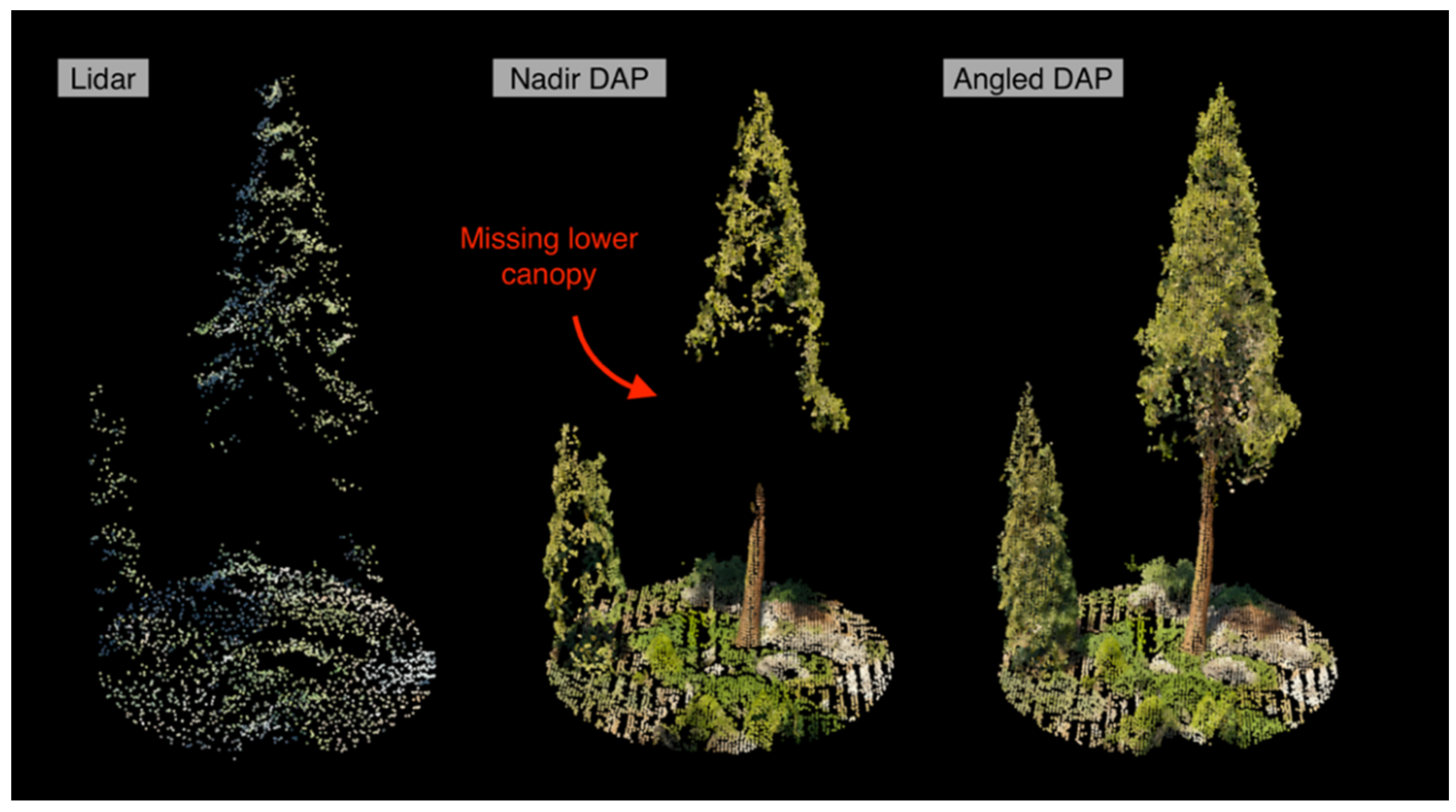
Additionally, many studies of UAS DAP have focused on individual forest types [24,27,33,34,35]. Assessment of DAP across a wide range of forest types and conditions is needed to develop best practices and enable the widespread application of UAS DAP in forest inventory and monitoring. Furthermore, standard practices of UAS DAP data acquisition typically include only collecting images at nadir, yet multi-angle DAP has potential in improving characterization of vertical forest structure [33]. By including off-nadir imagery in a DAP dataset, the image sensor has an increased view of the sides of the forest canopy, potentially allowing the photogrammetry algorithm to create a more “complete” model of the whole canopy than with nadir imagery alone [34,36,37,38]. An example of this can be seen in Figure 1, where the 3D DAP model generated with multi-angle imagery includes more of the lower tree canopy than nadir imagery alone. In combination, low-cost commercial-grade UAS, low-cost and user friendly HPGPS, and multi-angle (on and off-nadir) imagery have the potential for UAS DAP to be an affordable alternative to lidar for forest inventory, but have been largely unexplored.
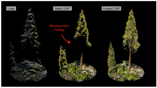
Figure 1.
Comparison of lidar, nadir DAP and off-nadir DAP 3D point clouds for a 0.05 ha circular plot in a Sierra Nevada mixed-conifer forest. Red arrow denotes missing structural elements in the lower canopy of the nadir DAP.
This study investigated if low-cost UAS DAP combined with low-cost HPGPS could generate digital surface models and predictions of select forest attributes with accuracy comparable to that of lidar. Specifically, three-dimensional point clouds were developed from imagery collected from a common low-cost commercial-off-the-shelf UAS platform and the imagery was georeferenced with ground coordinates collected using low-cost HPGPS. Study locations were selected to coincide with recent lidar data collection across multiple forest types and structural conditions in California, USA. 3D DAP was compared to lidar derived digital terrain models (DTMs), canopy height models (CHMs), and digital surface models (DSMs). Additionally, we compared DAP versus lidar modeled forest attributes based on field plot data. Specifically, we posed four research questions; (i) can low-cost UAS DAP imagery, combined with low-cost HPGPS, accurately generate surface models (DTMs, CHMs, and DSMs); and (ii) predict key and forest attributes (aboveground biomass, stem density, quadratic mean diameter, and mean tree height); (iii) how does accuracy of UAS 3D DAP vary across a wide range of forest conditions found throughout California; and (iv) can the introduction of off-nadir imagery improve the ability for UAS DAP to accurately model forest vegetation structure. We expected that UAS DAP would be able to create accurate surface models and predictions of forest attributes, although not as accurate as predictions made with lidar, and that UAS DAP accuracy will decline in dense forest canopies. We also expected that the addition of off-nadir imagery would consistently increase the accuracy of UAS DAP due to its potential to more completely characterize forest canopy structure.
2. Materials and Methods
2.1. Study Area
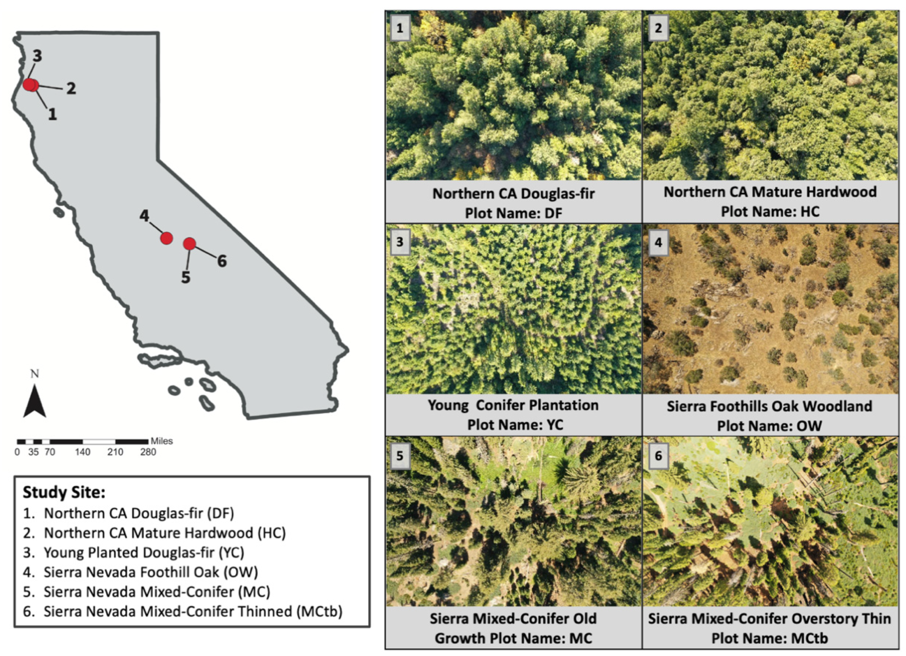
Study sites were selected based on availability of recent lidar in the State of California, desire to assess UAS 3D DAP across a wide range of forest types and structural conditions, and access to property for research activities. Study sites required available lidar data collected within two years prior to UAS imagery acquisition, restricting potential locations to those with available lidar data collected during 2017–2019. Sites also had to cover a range of forest conditions, including conifer and hardwood dominated sites, stand ages, and varying levels of canopy structural complexity. Lastly, sites had to be accessible, with landowners giving permission for research activities that included monumentation of plots and HPGPS base stations. Within these constraints, six different sites within California were chosen: northern California dense mature hardwood (HC), northern California mature Douglas-fir conifer (DF), Northern California young conifer (YC), Sierra Nevada foothill oak woodland (OW), old-growth Sierra Nevada mixed-conifer (MC), and a managed (thinned and burned) Sierra Nevada mixed-conifer forest (MCtb) (Figure 2). DF and HC sites are located within the L.W. Schatz Demonstration Tree Farm, managed by Humboldt State University. HC and DF are comprised of single and multi-aged patches with moderately tall trees and high canopy cover. The DF (40°46′40.37″N, 123°52′04.60″W) site is an approximately 40–60-year-old naturally established stand dominated by Douglas-fir (Pseudotsuga menziesii), with lesser components of grand fir (Abies grandis), and tanoak (Notholithocarpus densiflorus). The HC site contains two stands (40°46′31.73″N, 123°52′07.38”W and 40°46′02.87″N, 123°52′08.64″W) dominated by naturally established mature (over 80 years old) tanoak and California bay (Umbellularia californica), with less numerous Douglas-fir and grand fir. Both HC and DF overstories also include lesser amounts of Oregon ash (Fraxinus latifolia), red alder (Alnus rubra), big-leaf maple (Acer macrophylla), and pacific madrone (Arbutus menziesii). Understories for both HC and DF consist of younger cohorts of overstory conifers and hardwoods, along with smaller hardwood tree and shrub species such as pacific dogwood (Cornus nuttallii), willow (Salix spp.), and poison oak (Toxicodendron diversilobum). The YC site (40°47′54.35″N, 123°58′47.84″W) is owned and managed by Green Diamond Resource Company (Seattke, USA). YC has a low canopy characterized by evenly spaced trees, dominated by even-aged < 20-year-old planted Douglas-fir, with lesser components of naturally regenerated red alder, Oregon ash, grand fir, and tanoak. The understory consisted of brush and woody slash left over from a pre-commercial thinning conducted in 2017. The OW site (37°05′56.37″N, 119°44′05.89″W) is within the San Joaquin Experimental Range, operated by the USDA Forest Service Pacific Southwest Research Station. The OW site is dominated by naturally established blue oak (Quercus douglasii) and interior live oak (Quercus wislizeni), with a minor component of foothill pine (Pinus sabiniana) and California buckeye (Aesculus californica). OW has an open canopy with clumps of broad canopy hardwoods arising from multiple stems sprouting from common bases and a grassy understory. MC and MCtb are naturally established mixed conifer forests within Teakettle Experimental Forest, operated by the USDA Forest Service Pacific Southwest Research Station, and are part of a long-term thinning and prescribed fire experiment, established in 1997 [39]. The overstory at both sites is comprised of old-growth sugar pine (Pinus lambertiana), Jeffrey pine (Pinus jeffreyi) white fir (Abies concolor), and incense-cedar (Calocedrus decurrens). The oldest overstory pines exceed 400 years old, while the majority of shade tolerant fir and incense-cedar were established since the last recorded wildfire in 1865 [40]. The understory consists of younger cohorts of overstory species, dense patches of mountain whitethorn (Ceanothus cordulatus), bush chinquapin (Chrysolepis sempervirens), along with smaller populations of pinemat manzanita (Arctostaphylos nevadensis), green leaf manzanita (A. patula), and bitter cherry (Prunus emarginata). The MC site (36°57′54.23″N, 119°01′20.03″W) is unharvested old-growth with a moderately open canopy of tall uneven-aged conifers, resulting in high vertical and horizontal canopy complexity and large canopy gaps. The MCtb site (36°57′24.41″N, 119°01′11.75″W) was thinned from above in 2001, removing trees greater than 25 cm in diameter while retaining approximately 22 regularly spaced large diameter trees (> 100 cm) trees per hectare, resulting in a largely open canopy, low density of tall, large conifers, and dense shrub cover (largely Ceanothus cordulatus) up to 2 m tall. MCtb was also treated with prescribed burning in the fall of 2001 and fall of 2018 [40].
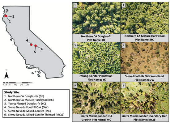
Figure 2.
Study site locations across California USA with associated UAS DAP images for each site. The UAS imagery was acquired at 120 m above ground level.
2.2. Field Data
Field data was collected in the summers of 2019 and 2020. We collected tree measurements in large stem maps to reduce the overall area for image acquisition, increase design control over forest composition and structural conditions, and to support a companion study assessing individual tree detection methods using 3D DAP. For each site, a 4-ha stem map was established, with the exception of the YC and HC sites. The YC site was limited to a single 2.3 ha stem map, due to the size of the continuous forest type and terrain surrounding the area. Due to the smaller patches of dense hardwood canopy at the HC site, two 2 ha stem maps were established, and we subsequently analyzed the data as one 4 ha area. In each stem map, all trees at least 5 cm diameter at breast height (DBH, 1.37 m) were measured and permanently monumented with numbered aluminum tags. Geographic coordinates of measured trees were collected at all but the MC and MCtb sites using low-cost ($1598 USD) Emlid RS+ real time kinematic (RTK) GPS receivers (Emlid Ltd., St. Petersburg, Russia). For each site, we established a base location with open sky conditions, and permanently monumented the location with a brass survey marker. The HPGPS receiver was then located 2 m above the survey marker on a tripod, and raw observation log data collected for at least one hour. Each base station log file was post-processed using the position and observation log of the nearest a local CORS reference station using the software package RTKLib [41] to calculate the position solution and accuracy for each base station. Post processed base stations were then used to correct our rover unit in real time (RTK) while collecting coordinates of trees. The two sites located within Teakettle Experimental Forest are part of an ongoing study with previously published stem maps generated using a surveyor total station [40,42]. The species, status (live versus snag), DBH, height, and crown class (dominant, co-dominant, intermediate, and suppressed) were recorded for each tree. Within each stem map, a minimum of twenty 12.62 m radius (0.05 ha) fixed area plots were systematically sampled using a hexagonal lattice, with a minimum distance between plot centers of 26.9 m to avoid tree stem overlap. Live trees were extracted for each plot, and density (TPH), basal area (BA, m2), quadratic mean diameter (QMD, cm), Lorey’s mean height (LHT, m), and aboveground biomass (AGB, Mg/ha) calculated for each plot (Table 1). Aboveground live biomass was calculated using generalized biomass equations [43].

Table 1.
Summary statistics of plot-level forest attributes at each site calculated from field data.
2.3. Lidar Data
Lidar data was collected for all study sites in 2018 and 2019. Lidar for MC, MCtb, and OW sites were collected in the summer of 2018 by the National Ecological Observatory Network Airborne Observation Platform (NEON AOP, https://www.neonscience.org/data/airborne-data, accessed on 19 November 2020). Lidar for the YC site was collected by Quantum Spatial Inc. (Sheboygan Falls, WI, USA) in the summer of 2018 as part of a larger data acquisition for Green Diamond Resource Company. Lidar data for the DF and HC sites was collected in the Fall of 2019 by Access Geographic LLC (Tempe, AZ, USA) as part of a larger acquisition for the cities of Eureka and Arcata, California. Lidar data was collected with different sensors and acquisition parameters, resulting in dramatically different point densities (Table 2) To reduce the potential impact of differing point cloud densities, lidar point clouds were filtered to be comparable with our lidar point clouds with the lowest point densities using the decimation function and the homogenize algorithm in lidR [44], resulting in point cloud densities 5.4–12.3 pts/m2.
Table 2.
Site specific lidar acquisition specifications.
2.4. UAS DAP Data
UAS DAP imagery was collected in the summer of 2019 from a DJI Mavic 2 Pro (DJI, Shenzhen, China, $1500 USD). The Mavic 2 Pro has a 1-inch CMOS image sensor that collects high-resolution still images (5472 × 3648 pixels) in the red, green, and blue (RGB) visual light spectrum with a field of view of 77 degrees. The camera is attached to the UAS by a 3-axis gimbal, allowing control of the angle at which the images are taken. UAS flights were planned using flight planning software Map Pilot version 4.0.1 (Drones Made Easy, CA, USA), and geotagged images were taken along the flight paths using the internal GPS within the UAS. Although Map Pilot has the ability to use terrain models developed from lidar to create missions that follow the elevational profile of the terrain, a major objective of this study was to assess low-cost DAP for locations that had no previous lidar data collected. Missions were flown 120 m above terrain level using the 30 m digital elevation model from the Shuttle Radar Topography Mission (SRTM, NASA). Flight paths, in parallel transects, were set with 85% front and 85% side overlap between adjacent images [36,37]. Some studies show that a gridded flight path is preferred when using angled imagery [45,46,47], giving the UAS a view of the canopy from four perspectives; however, due to study area size and battery limited flight time constraints we chose to use parallel transects. We also did not want to complicate the comparison between nadir and angled DAP models by collecting the two sets of imagery in a different manner. Mission boundaries were set approximately 20 m outward from site boundaries to avoid edge effects. Two missions were flown over each site, one with images taken at nadir and the other with images taken 30 degrees off nadir. Previous studies recognized greater than 80% overlaps and 15 to 45 degrees of tilted camera as desired options for canopy tree studies [36,37,38]. All missions were flown on days with little to no cloud cover, minimal wind and near local solar noon, with the exception OW which was flown later in the afternoon (approximately 2:00 p.m. local time) due to concerns of heat impacts on UAS batteries.
UAS imagery was processed to generate 3D point clouds using Agisoft Metashape Professional version 1.5.4 (Agisoft LLC, St. Petersburg, Russia). This program utilizes the photogrammetric method for 3D reconstruction of overlapping photographs. SfM is a photogrammetric range imaging technique that matches features in offset images from multiple overlapping using bundle adjustment procedures. The initial image alignment was done using the “High” accuracy setting, allowing the program to use the full resolution of each photo when selecting matching points. Each image taken from the UAS image sensor was geospatially tagged by the drones internal GPS. This GPS data is utilized to assist in the image alignment process, but due to the low accuracy of the internal GPS, UAS images were georectified using eleven ground control points (GCPs, 12-inch-wide black and white tiles) placed throughout the flight area at each study site, with their coordinates precisely measured with an HPGPS following the same methods as described above to collect coordinates for trees in stem maps. Once the initial image alignment was completed, the UAS GPS data was no longer referenced and only the GCPs were used to georeference the generated models. A dense point cloud was then generated using the “High” accuracy setting allowing the use of each image’s full resolution when locating matching points between photos. This resulted in a high-density point cloud of approximately 250 pts/m2. Due to computational requirements associated with analysis of such high point densities, point clouds were filtered to a voxel spacing of 0.05 m3 between points, resulting in densities of approximately 50 pts/m2 without degrading structural characteristics in the point clouds.
2.5. Lidar and DAP Point Cloud Processing
Lidar and DAP derived point clouds were processed using the lidR package [44] in R [48]. All point clouds were clipped to the boundaries of the sites plus a 20 m buffer to avoid edge effects during processing. Ground points were classified using the cloth simulation filter (csf) algorithm [49]. Digital terrain models (DTMs) were generated from classified ground points using a Delaunay triangulation algorithm [50]. Digital surface model (DSMs) were generated using the pitree algorithm [51]. Point clouds were then normalized using the DTMs for the given model at each site. Canopy height models (CHMs) were then generated from the normalized point clouds using the same pitree algorithm as for the DSMs. All DSMs, DTMs, and CHMs were regenerated as rasters with a 1 m resolution.
For predicting forest attributes, normalized point clouds were clipped to the same 0.05 hectare fixed-area plots previously described in Field Data section above. Point cloud summary statistics were derived from the point cloud for each plot. These metrics included max height (zmax), mean height (zmean), standard deviation of height (zsd), skewness of height distribution (zskew), kurtosis of height distribution (zkurt), entropy of height distribution (zentropy) [52], percentage of returns above mean height (pzabovemean), percentage of returns above 2 m (pzabove2), quantiles of height from 5 to 95 in 5% increments (zq5-95), and the cumulative percentage of returns (zpcum1-9).
2.6. Statistical Analyses
All statistical analyses were conducted in R [49]. For each gridded surface model (DTM, DSM, and CHM) we compared both UAS DAP-derived (nadir and off-nadir) pixel values for the model against the lidar-derived version for each site separately. In this study, the term accuracy is used to describe how close models from UAS DAP are compared to predictions and observations made by the standard collection method most used in forest inventory. For 3D data products, such as digital surface models, lidar is the most accurate source whereas ground collected field data from fixed or variable radius plots are used in the collection of forest structural attributes, such as tree heights and basal area. To determine how accurately UAS DAP predictions compared to predictions made from lidar and observed field data, this study followed many of the accuracy assessment protocols for continuous variables as described by Riemann et al. [53]. R-squared, root mean square deviation (RMSD), normalized RMSD (nRMSD), agreement coefficient (AC), systematic agreement coefficient (ACsys) and unsystematic agreement coefficient (ACuns) were calculated between UAS DAP and lidar derived surface models.
For predictions of forest attributes, plot values of AGB, BAH, TPH, QMD, and LHT were predicted using the summary statistics from lidar and DAP models for each plot. Multiple linear regressions were developed for each forest attribute using all plots across sites. Global predictions, across all sites, were chosen instead of site-specific predictions due to the limited number of samples and the amount of predictor variables being tested. Although this could lower overall site-specific accuracies due to variability of stand structure between sites, the global model allowed us to make predictions on stand structure using more than one predictor variable. The forest attribute variables were first checked for linearity and normality using histograms and Q-Q plots, resulting in AGB data being cube root transformed, while BAH, TPH, QMD, and LHT were square root transformed. The leaps package in R [54] was used to determine the best subsets of predictor variables for regression models for each forest attribute. The maximum number of predictor variables in a model was set to five, and the best model from candidate models was determined by adjusted R2 and BIC values. These models were then used to predict plot-level AGB, BAH, TPH, QMD, and LHT using the derived structural metrics from lidar and DAP models for each plot at each site using leave one out cross validation (LOOCV) with the caret package [55]. With LOOCV, where N is equal to the number of samples, the model is trained on all the data with the exception of one plot and a prediction is made for that plot. In our case the number of instances (plots for each site) varied by site (n = 20–26). Given the small sample size per site, LOOCV may be preferable to classical training-validation splits and k-fold cross validation approaches, as no sampling of the training dataset is used in LOOCV (i.e., each plot is predicted with the plot reserved from the model). This means the LOOCV estimation procedure is deterministic compared to training-validation splits and k-fold cross validation that can have a more stochastic estimate of model performance with small sample sizes. Cross-validated predictions of plot-level forest attributes made by each best fit model were compared to that of observed forest attributes computed from field data.
3. Results
3.1. Accuracy of UAS DAP Surface Models
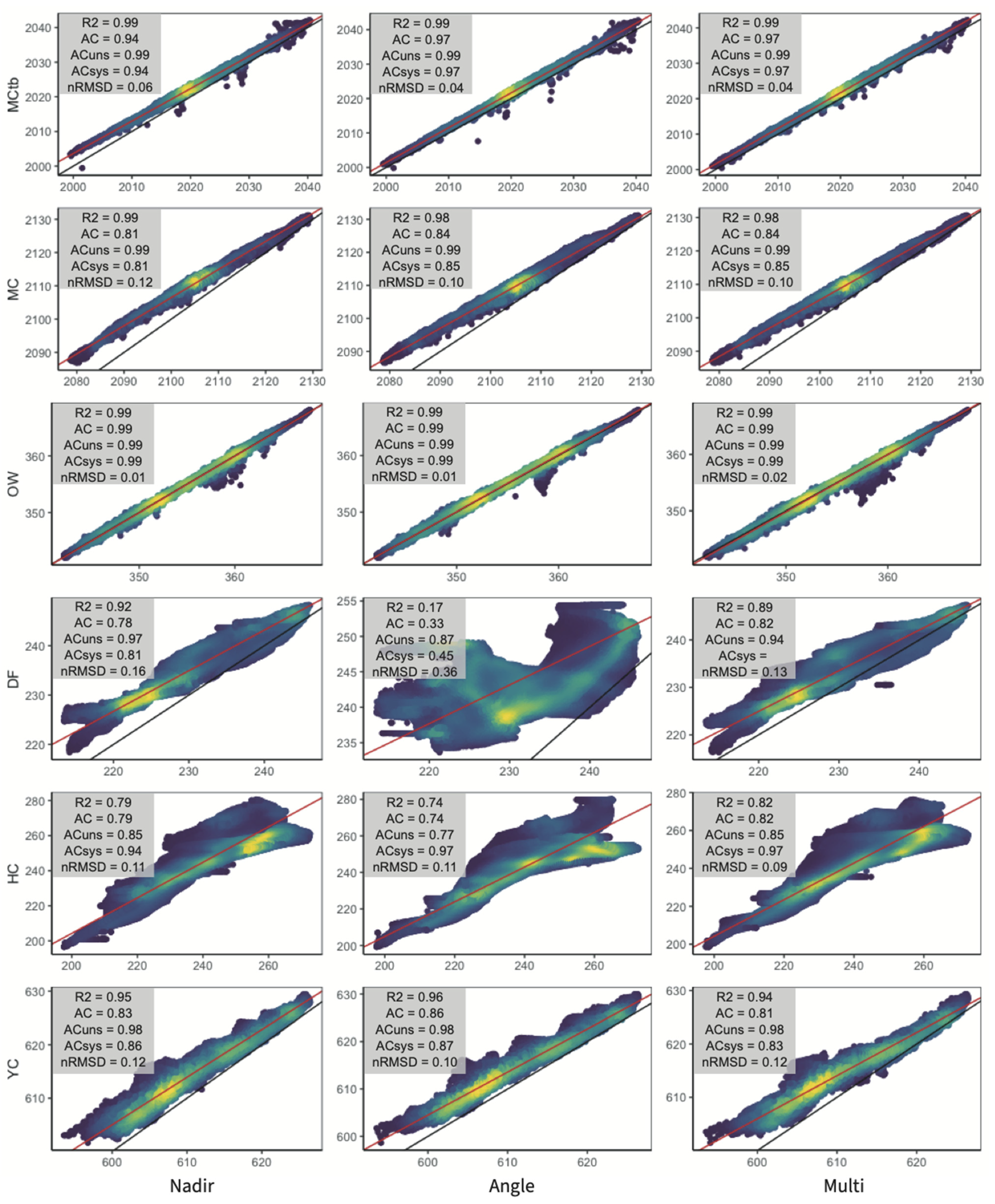
Digital terrain models (DTMs) derived from UAS DAP displayed high correlation compared to lidar DTMs, with R2 values ranging from 0.74 to 0.99 (Figure 3). The exception was the DTM using off-nadir imagery at the Douglas-fir (DF) site, with an R2 of only 0.01 compared to the lidar DTM. R2 of UAS DAP DTMs in relation to lidar DTMs was lower for sites with denser canopy cover and rougher terrain. Nadir imagery DTMs performed best when compared to lidar DTMs, with systematic agreement (ACsys) values above 0.8 and unsystematic agreement (ACuns) values above 0.85. DTMs from nadir imagery also showed the highest amount of agreement when compared to lidar DTMs, with AC values above 0.78 (Figure 3).

Figure 3.
Comparison of site-specific digital terrain models (DTM) generated from UAS DAP (nadir, angled, and multi-angled) versus lidar. The X axis is DAP and the Y axis is lidar. Geometric mean fit regression line in red, 1:1 line in black, points are colorized by density of observations (i.e., number of raster pixels) with lighter regions (yellow) indicating greater density of observations and darker regions (blue) being less dense. R-squared, root mean square deviation (RMSD), normalized RMSD (nRMSD), agreement coefficient (AC), systematic agreement coefficient (ACsys) and unsystematic agreement coefficient (ACuns) are shown for each model comparison.
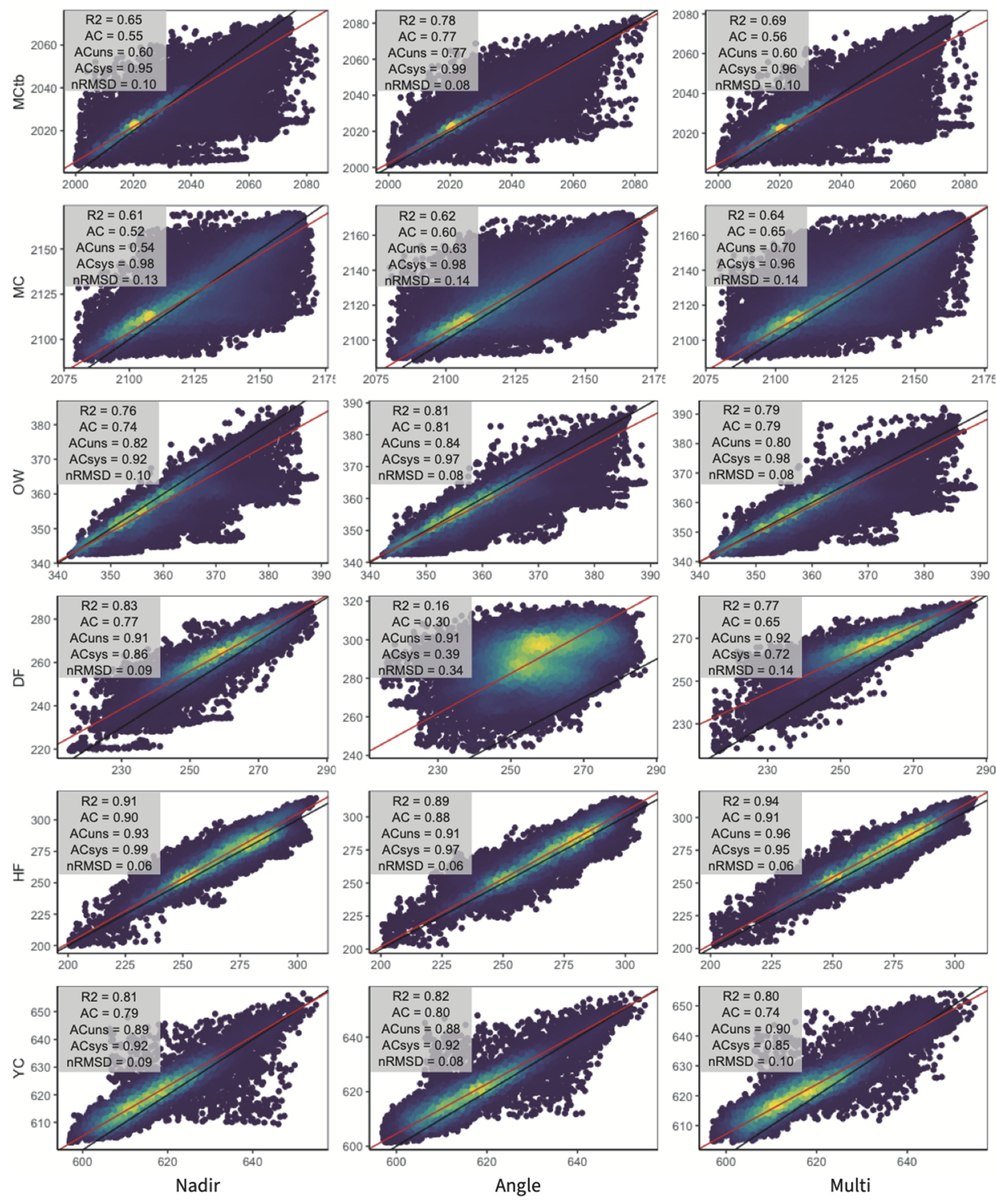
DSMs and CHMs from UAS DAP tended to show less agreement with lidar compared to DTMs. At sites with dense canopy cover, DSMs and CHMs from only angled imagery showed less correlation and lower levels of agreement when compared DSMs and CHMs from lidar. UAS DAP CHMs had low correlations with lidar CHMs, showing poorest results at sites with tall, dense canopies, and this was especially problematic when using off-nadir imagery (Figure 4 and Figure 5).
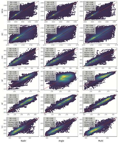
Figure 4.
Comparison of site-specific digital surface models (DSM) generated from UAS DAP (nadir, angled, and multi-angled) versus lidar. The X axis is DAP and the Y axis is lidar. Geometric mean fit regression line in red, 1:1 line in black, points are colorized by density of observations (i.e., number of raster pixels) with lighter regions (yellow) indicating greater density of observations and darker regions (blue) being less dense. R-squared, root mean square deviation (RMSD), normalized RMSD (nRMSD), agreement coefficient (AC), systematic agreement coefficient (ACsys) and unsystematic agreement coefficient (ACuns) are shown for each model comparison.

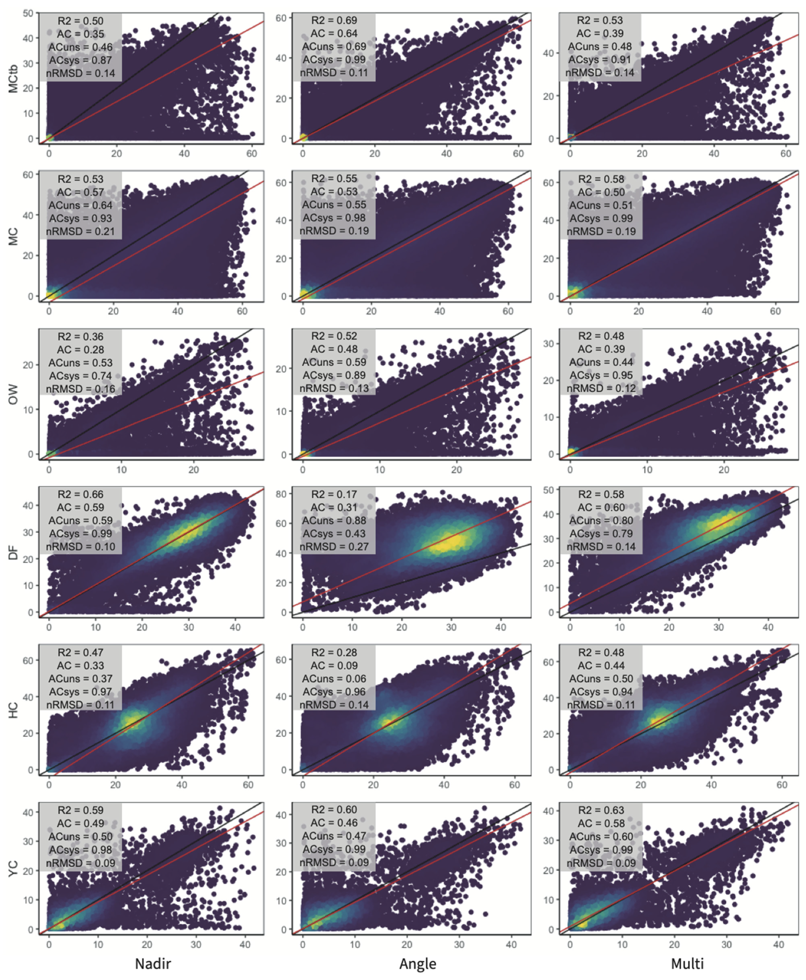
Figure 5.
Comparison of site-specific canopy height models (CHM) generated from UAS DAP (nadir, angled, and multi-angled) versus lidar. The X axis is DAP and the Y axis is lidar. Geometric mean fit regression line in red, 1:1 line in black, points are colorized by density of observations (i.e., number of raster pixels) with lighter regions (yellow) indicating greater density of observations and darker regions (blue) being less dense. R-squared, root mean square deviation (RMSD), normalized RMSD (nRMSD), agreement coefficient (AC), systematic agreement coefficient (ACsys) and unsystematic agreement coefficient (ACuns) are shown for each model comparison.
3.2. Accuracy of UAS Forest Attribute Predictions
Best-fit plot-level regression models resulted in good predictive ability when using metrics derived from both lidar and SfM point clouds (Table 3). UAS DAP models had similar prediction performance to lidar-based predictions, with the exception of the off-nadir DAP models prediction of QMD (R2 = 0.45). The strongest predictor variables used when estimating AGB, TPH, BAH and LHT tended to be zmean, zsd, and pzabove2 while models predicting QMD tended to rely on quartile metrics. All model predictions showed moderate to high correlation (R2 = 0.53–0.84) to observed values of AGB, THP, BAH, and LHT (Table 4, Figure 6). Overall, regression models using lidar derived predictor variables were more accurate than models of the same response variables using UAS DAP derived predictors, with the exception of the model of QMD using nadir UAS DAP predictor variables (R2 = 0.70). UAS DAP models containing off-nadir images (both off-nadir and multi-angled models) tended to have marginally higher correlation values and marginally lower RMSD and nRMSD values, compared to nadir based models.
Table 3.
Summary of plot-level regression models of forest attributes using lidar and DAP predictor variables.
Table 4.
Comparisons of plot-level observed forest metrics to predictions made by lidar and UAS DAP models.
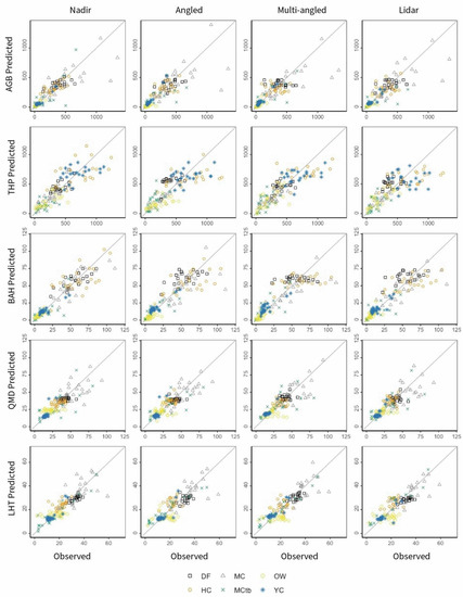
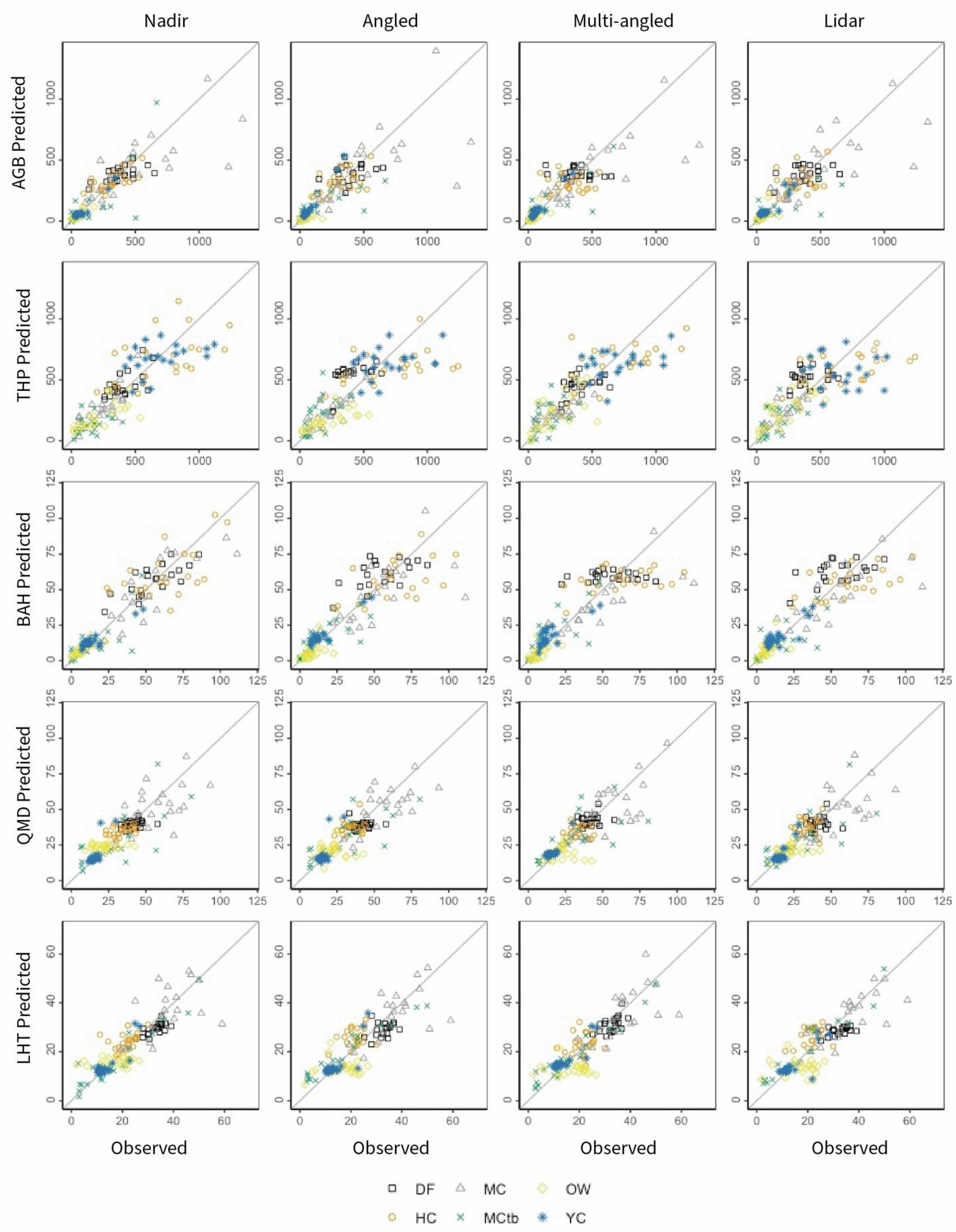
Figure 6.
Observed vs. predicted plot-level estimates of AGB, TPH, BAH, QMD, and LHT. Solid line displayed is the 1:1 line. Plots color coded by site.
When comparing predicted forest attributes for all sites between the UAS DAP and lidar, all UAS DAP predictions were highly correlated with lidar predictions (Table 5). UAS DAP models containing only off-nadir images were shown to have the highest correlations with lidar-based predictions (R2 = 0.75–0.85), with the exception of QMD predictions. Multi-angle UAS DAP models containing both nadir and off-nadir images had slightly poorer performance when compared to lidar, with R2 values ranging from 0.66 to 0.83.
Table 5.
Comparisons of plot-level forest metric predictions made by lidar to those of UAS DAP.
4. Discussion
Until recently, low-cost UAS DAP has been viewed as a low-quality 3D data source, in part due to low quality onboard GPS and associated positional errors of imagery. Through comparison of UAS DAP and lidar derived surface models and plot-level forest metrics predictions, this study shows that low cost UAS, when combined with low-cost HPGPS, can predict key forest metrics across a wide range of forest types and conditions with moderate accuracy. However, the accuracy of UAS DAP surface models can vary greatly by the type of surface model (DSM, DTM, or CHM), as well as forest type and structural characteristics. In contrast to surface models, less variability was observed in UAS DAP predictions of plot-level forest attributes. The use of off-nadir imagery only provided marginal improvements to UAS DAP surface models and predictions of forest attributes, and in the case of tall and dense forest canopies, the use of off-nadir image negatively affected the model accuracy. Our results suggest the integration of low-cost UAS DAP with HPGPS can provide accurate 3D data and forest attribute estimation in many forest types and structural conditions, but key limitations and uncertainties remain. Below, we discuss the possible causes of variability in UAS DAP generated digital surface models and predicted forest attributes, provide suggestions as to how low-cost UAS DAP can be utilized in forest inventory and monitoring applications, and potential limitations and future questions resulting from our findings.
4.1. UAS Surface Models
In previous studies, UAS DAP was aided by integration of lidar generated terrain models to normalize the DAP point clouds and create CHMs [26,33,56,57,58,59]. This, however, means low-cost DAP still required a high cost lidar acquisition, cost prohibitive for smaller studies sites and small landowners without lidar data. In our study, surface models generated from UAS DAP were found to have high levels of agreement compared to those generated from lidar, with decreased levels of accuracy in DSMs and CHMs. Reduced accuracy of DSMs and CHMs was especially pronounced at our mature Douglas-fir and hardwood site characterized by high canopy cover with few canopy gaps, resulting in the occlusion of the terrain from the UAS passive optical sensor, leaving larger data gaps above the modeled terrain, an important element when generating accurate CHMs. Visualizations of the UAS DAP and lidar point clouds show fewer classified ground points in locations with dense canopies (Figure 7), consistent with observations made in previous studies [60,61,62]. This became most problematic with off-nadir DAP models with dense canopies at the Douglas-fir site, where there were not enough matched ground points to accurately model the terrain due to heavy canopy occlusion, resulted in an R2 value of 0.17 when compared to the terrain model generated from lidar (Figure 4).
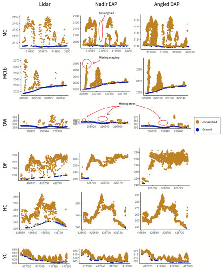
Figure 7.
Point clouds from lidar, nadir DAP and angled DAP shown as 70 m transects for each site and colored by classification. The different sites are shown on the vertical axis with different model types on the horizontal axis. Arrows show missing canopy data or, in the case of MCtb, the missing top of a standing dead tree (snag).
4.2. Accuracy of UAS Forest Metric Predictions
When comparing UAS DAP versus lidar predictions of plot-level forest attributes, lidar-based models consistently had the highest overall accuracy, while UAS DAP based models had slightly lower accuracies. It was expected that models generated with only off-nadir imagery would show poorer results in predicting forest metrics due to the relatively lower levels of agreement found in the surface model comparisons; however, angled models were shown to have equal, and in some cases marginally better, performance than nadir and multi-angled DAP model predictions of aboveground live biomass, stand density, and Loreys mean height. A possible explanation for accurate plot-level forest attribute predictions without having an accurate terrain model comes from the research of Giannetti et al. [63]. Their results show that accurate predictions of forest metrics can be made from UAS DAP without the need for point cloud normalization from a DTM. When off-nadir DAP model predictions were compared to lidar model predictions, they only had marginal improvements over nadir and multi-angled models for all forest attributes, with the exception of quadratic mean diameter (QMD). All UAS DAP model predictions, however, were shown to have a high correlation to lidar predictions. Another option for normalization of DAP point clouds is to use publicly available national or global elevation data sources such as the USGS 3D Elevation Program (3DEP), NASA Shuttle Radar Topography Mission (SRTM), or JAXA Advanced Land Observing Satellite (ALOS). While these publicly available elevation datasets can be a potential source of terrain data in cases of high canopy cover, they tend to be coarse resolution (generally 10–30 m), which could lead to potential vertical errors in areas with high canopy cover and topographic variability [64,65,66]. Estimates of wood volume (and therefore aboveground biomass and carbon) may be highly sensitive to error in vegetation height [67]. We did not want potential error in publicly available DTMs to confound our evaluation of UAS DAP, so UAS DAP point cloud normalization used UAS DAP generated DTMs.
4.3. Value of Off-Nadir Imagery in DAP Surface Models and Forest Attribute Predictions
In DAP generated surface models, the use of angled imagery included some of the structural information that the nadir DAP missed. However, it was also apparent that in off-nadir imagery for sites with dense canopies, the ground was completely occluded in most images, resulting in very few GCPs being seen and potentially leading to higher georeferencing error in the associated DAP surface models. Similarly, Lovitt et al. [68] reported high root mean square error (40 cm RMSE) for the areas of complex microtopographic terrain with thick vegetation canopies in peatlands. However, accuracy can be improved with post processed differential GPS correction even with a few ground control points for registering images [36,60]. This was improved with the re-introduction of nadir images in the multi-angled model. It was thought that by including both nadir and off-nadir images in our DAP models, which both increases the amount of viewing angles of the canopy while also essentially doubling the number of images in which to create matching points from, that the resulting surface models would be more complete and representative of stand structure. However, multi-angle imagery did not increase the overall accuracy of surface models or predictions of forest attributes compared to models based on nadir DAP. In the plot-level predictions, off-nadir imagery developed models that were marginally better able to predict forest attributes. This was most apparent comparing angled DAP versus lidar based model predictions. Nadir DAP sometimes omitted trees at sites characterized by open canopies and large isolated trees (Figure 4 and Figure 5). Given the marginal gains of angled imagery, and the time required for data collection and processing of both angles and nadir imagery, nadir imagery should be the default for UAS DAP surface model generation and forest attribute prediction, with angled image collection restricted to forests with open canopy conditions that are not prone to occlusion of the terrain form the image sensor.
4.4. Limitations
There was poor agreement between DSMs and CHMs generated from UAS DAP and lidar (Figure 3 and Figure 5). This may be caused by slight shifts in the georeferencing of UAS DAP rather than missing or erroneous values. While coupling our UAS DAP with low-cost HPGPS, high canopy cover and density can still increase GPS error of ground control points. This may have shifted the UAS DAP coordinates, lowering the overall agreement between 1 m pixels. Another source of potential error in CHMs and DSMs can be seen in UAS DAP modeling of complex canopies in our Sierra Nevada mixed conifer sites and open canopy in our oak woodland site. It was expected that these sites would perform well given better observational ability of passive optical sensors with reduced canopy cover and terrain occlusion. However, DAP models of these sites had missing canopy structural data (Figure 1 and Figure 6). One cause for this could be the use of aggressive depth filtering in photogrammetric processing to remove outlier point observations resulting from poor imagery or bad alignment issues. The use of aggressive depth filtering in the generation of UAS DAP point clouds may lead to the filtering segments of the forest canopy as noise, and lower depth filtering settings could be used when modeling forest canopies [69].
Lidar marginally outperformed UAS DAP when predicting plot-level forest attributes. Lidar has traditionally been the preferred remotely sensed data for characterizing ground terrain and vertical forest structure in support of forest inventory and monitoring. However, airborne lidar data is cost prohibitive for small areas and frequent data collection. Under specific forest conditions, our study found that low-cost UAS DAP can generate similar data products to lidar in a less expensive, flexible, and rapidly deployable manner. Land managers can utilize UAS DAP in forest inventory and monitoring to generate high resolution imagery, 3D models, and forest attribute prediction without the need for previously collected DTMs from lidar.
UAS DAP has also been shown to have limitations due to its use of passive imagery. DTMs generated from UAS DAP in dense, closed canopy forest conditions show lower levels of agreement than in sites with more open conditions. Although we show that UAS DAP can make accurate predictions of forest attributes, the spatial variation and bias in UAS DAP surface models at all sites suggests caution in using UAS DAP when doing pixel-to-pixel comparisons. It also suggests that utilizing lidar generated DTMs when normalizing UAS DAP DSMs in dense canopy conditions might still be necessary to create accurate CHMs. Our study evaluated the accuracy of gridded surface models and plot-level predictions, data sources and methods underpinning area-based estimation [70]. However, a weakness of area-based approaches is many different 3D point cloud derived metrics can be used to construct multiple regression equations, so they often require local fine-tuning and may not be applicable beyond the study sites or region in which they were calibrated. We found equivocal evidence of broader model utility across a range of forest types, with relatively high accuracy of predicted forest attributes across forest types with different dominant species and structural conditions. At the same time, strong differences in the accuracy of UAS DAP canopy height models in tall dense canopies suggests limitations for development of consistent area-based models using UAS DAP, especially given estimation of some key forest attributes can be highly sensitive to vegetation height from remotely sensed data [68]. Alternatively, individual tree detection may have numerous advantages over area-based approaches [71], such as the following: similarity to field-based allometric approaches, reduced dependence on plot size, narrow patches of forest with high conservation value can be mapped, and repeat 3D data could in principle allow for the quantification of growth and mortality for individual trees. Using UAS DAP in an individual tree detection-based forest inventory may be especially attractive, as its high point cloud density may me more important for individual tree detection accuracy versus area-based approaches [72]. Although beyond the scope of our study and its findings, the benefits of high point densities of UAS DAP in individual tree detection is an area of research warranting investigation. Lastly, current methods of using lidar and UAS DAP point clouds in forest inventory lack the ability to determine species level data. Photogrammetric point clouds can, however, integrate spectral information from the image sensors into the generated point clouds. This added spectral information could allow for additional predictive power in UAS DAP to make predictions of species and forest health as well as forest structural attributes [59].
5. Conclusions
This study demonstrates that low-cost, commercial-grade UAS DAP coupled with new-to-market, low-cost HPGPS can generate comparable data products and predictions to lidar and field observations of forest attributes across a wide range of forest sites and conditions. The addition of off-nadir imagery into UAS DAP models only marginally affects the accuracy of surface model and forest attribute predictions. Comparisons of UAS DAP versus lidar based surface models indicates the need for previously acquired lidar terrain models may not be necessary to achieve accurate CHMs from photogrammetry models except in forests with tall dense canopies, and for all forest types UAS DAP predictions of forest attributes can be comparable to lidar.
UAS DAP can be both an affordable and accurate remote sensing tool in forest inventorying and monitoring. With a combined cost of under $5000 USD, the equipment and software used in this study represent a dramatically lower fixed cost versus an airborne lidar sensor and aircraft, fuel, pilot, and supporting ground personnel. As such, integration of low cost UAS DAP and HPGPS can provide time and place flexible data for small area inventory and forest attribute estimation not possible with lidar data. Forest managers should consider the structural characteristics of the forest of interest when determining whether UAS DAP is an appropriate data source, and if they should include off-nadir images in their UAS data acquisition. For use in continuous forest inventory and monitoring programs, UAS DAP can make accurate predictions of forest stand attributes; however, it may not have the spatial accuracy to make direct comparisons of generated surface models between data collection periods depending on forest canopy density.
Author Contributions
Conceptualization, H.S.J.Z. and J.E.L.; methodology, H.S.J.Z.; validation, H.S.J.Z. and J.E.L.; formal analysis, J.E.L. and H.S.J.Z.; resources, H.S.J.Z.; data curation, J.E.L.; writing—original draft preparation, J.E.L.; writing—review and editing, H.S.J.Z., B.D.M. and J.G.; supervision, H.S.J.Z. and J.G.; project administration, H.S.J.Z. and J.G.; funding acquisition, H.S.J.Z. All authors have read and agreed to the published version of the manuscript.
Funding
Funding for this research was provided by the California State University Agricultural Research Institute (Grant 20-06-100) and the L.W. Schatz Demonstration Tree Farm. Measurement of stem maps at Teakettle Experimental Forest was in part supported by the Joint Fire Science Program (Grant 15-1-07-6).
Data Availability Statement
Lidar data used in this study for Teakettle Experimental Forest and the San Joaquin Experimental Range are openly available from the National Ecological Observatory at https://data.neonscience.org/data-products/explore (accessed on 22 August 2021). Lidar, UAS DAP, and field data presented in this study are available on request from the corresponding author. These data (except for lidar at Teakettle Experimental Forest and the San Joaquin Experimental Range) are not publicly available due to companion research project still in progress. Restrictions apply to the availability of all geospatial collected on Green Diamond Resource Company lands, and are only available with the expressed consent of Green Diamond Resources Company.
Acknowledgments
Special thanks Daniel Jones and Alex Pickering for assisting in field data collection. Also, thanks to the L.W. Schatz Demonstration Tree Farm field crews for assisting in data collection. The authors would also like to acknowledge Green Diamond Resource Company and David Lamphear for access to both their land and to their most recent lidar data. We also thank the U.S. Forest Service for access to both the Teakettle Experimental Forest and San Joaquin Experimental Range, and to NEON for open access to the lidar data for Teakettle Experimental Forest and San Joaquin Experimental Range. Additional thanks to Marissa Goodwin for work on the Teakettle Experimental Forest stem map. Lastly, we thank three anonymous reviewers, whose insightful and constructive comments greatly improved this manuscript.
Conflicts of Interest
The authors declare no conflict of interest.
References
- Bechtold, W.A.; Patterson, P.L. The Enhanced Forest Inventory and Analysis Program-National Sampling Design and Estimation Procedures; Bechtold, W.A., Patterson, P.L., Eds.; USDA Forest Service, Southern Research Station: Asheville, NC, USA, 2015; Volume 80, pp. 27–42.
- Gillis, M.D.; Omule, A.Y.; Brierley, T. Monitoring Canada’s forests: The national forest inventory. For. Chron. 2005, 81, 214–221. [Google Scholar] [CrossRef]
- Tomppo, E.; Gschwantner, T.; Lawrence, M.; McRoberts, R.E. National Forest Inventories: Pathways for Common Reporting; Springer: Amsterdam, The Netherlands, 2010; ISBN 9789048132324. [Google Scholar]
- Wulder, M.A.; Kurz, W.A.; Gillis, M. National level forest monitoring and modeling in Canada. Prog. Plann. 2004, 61, 365–381. [Google Scholar] [CrossRef]
- Rao, J.N.K. Small-Area Estimation. In Wiley StatsRef: Statistics Reference Online; John Wiley & Sons, Ltd.: Chichester, UK, 2017; pp. 1–8. [Google Scholar]
- Ohmann, J.L.; Gregory, M.J. Predictive mapping of forest composition and structure with direct gradient analysis and nearest-neighbor imputation in coastal Oregon, U.S.A. Can. J. For. Res. 2002, 32, 725–741. [Google Scholar] [CrossRef]
- Tomppo, E.; Olsson, H.; Ståhl, G.; Nilsson, M.; Hagner, O.; Katila, M. Combining national forest inventory field plots and remote sensing data for forest databases. Remote Sens. Environ. 2008, 112, 1982–1999. [Google Scholar] [CrossRef]
- Wilson, B.T.; Woodall, C.W.; Griffith, D.M. Imputing forest carbon stock estimates from inventory plots to a nationally continuous coverage. Carbon Balance Manag. 2013, 8, 1. [Google Scholar] [CrossRef] [Green Version]
- Drusch, M.; Del Bello, U.; Carlier, S.; Colin, O.; Fernandez, V.; Gascon, F.; Hoersch, B.; Isola, C.; Laberinti, P.; Martimort, P.; et al. Sentinel-2: ESA’s Optical High-Resolution Mission for GMES Operational Services. Remote Sens. Environ. 2012, 120, 25–36. [Google Scholar] [CrossRef]
- Kennedy, R.E.; Andréfouët, S.; Cohen, W.B.; Gómez, C.; Griffiths, P.; Hais, M.; Healey, S.P.; Helmer, E.H.; Hostert, P.; Lyons, M.B.; et al. Bringing an ecological view of change to landsat-based remote sensing. Front. Ecol. Environ. 2014, 12, 339–346. [Google Scholar] [CrossRef]
- Wu, Z.; Dye, D.; Vogel, J.; Middleton, B. Estimating Forest and Woodland Aboveground Biomass Using Active and Passive Remote Sensing. Photogramm. Eng. Remote Sens. 2016, 82, 271–281. [Google Scholar] [CrossRef]
- Turner, D.P.; Cohen, W.B.; Kennedy, R.E.; Fassnacht, K.S.; Briggs, J.M. Relationships between Leaf Area Index and Landsat TM Spectral Vegetation Indices across Three Temperate Zone Sites. Remote Sens. Environ. 1999, 70, 52–68. [Google Scholar] [CrossRef]
- Lu, D. The potential and challenge of remote sensing-based biomass estimation. Int. J. Remote Sens. 2006, 27, 1297–1328. [Google Scholar] [CrossRef]
- Pierce, K.B.; Ohmann, J.L.; Wimberly, M.C.; Gregory, M.J.; Fried, J.S. Mapping wildland fuels and forest structure for land management: A comparison of nearest neighbor imputation and other methods. Can. J. For. Res. 2009, 39, 1901–1916. [Google Scholar] [CrossRef]
- Zald, H.S.J.; Ohmann, J.L.; Roberts, H.M.; Gregory, M.J.; Henderson, E.B.; McGaughey, R.J.; Braaten, J. Influence of lidar, Landsat imagery, disturbance history, plot location accuracy, and plot size on accuracy of imputation maps of forest composition and structure. Remote Sens. Environ. 2014, 143, 26–38. [Google Scholar] [CrossRef]
- Eskelson, B.N.I.; Temesgen, H.; Hagar, J.C. A comparison of selected parametric and imputation methods for estimating snag density and snag quality attributes. For. Ecol. Manage. 2012, 272, 26–34. [Google Scholar] [CrossRef]
- Dubayah, R.O.; Drake, J.B. Lidar Remote Sensing for Forestry Applications. J. For. 2000, 98, 44–46. [Google Scholar]
- Lefsky, M.A.; Cohen, W.B.; Parker, G.G.; Harding, D.J. Lidar Remote Sensing for Ecosystem Studies: Lidar, an emerging remote sensing technology that directly measures the three-dimensional distribution of plant canopies, can accurately estimate vegetation structural attributes and should be of particular inte. Bioscience 2002, 52, 19–30. [Google Scholar] [CrossRef]
- Reutebuch, S.E.; Andersen, H.; Mcgaughey, R.J. Light Detection and Ranging (LIDAR): An Emerging Tool for Multiple Resource Inventory. J. For. 2005, 103, 286–292. [Google Scholar] [CrossRef]
- Andersen, H.E.; Strunk, J.; Temesgen, H.; Atwood, D.; Winterberger, K. Using multilevel remote sensing and ground data to estimate forest biomass resources in remote regions: A case study in the boreal forests of interior Alaska. Can. J. Remote Sens. 2012, 37, 596–611. [Google Scholar] [CrossRef]
- Wulder, M.A.; White, J.C.; Nelson, R.F.; Næsset, E.; Ørka, H.O.; Coops, N.C.; Hilker, T.; Bater, C.W.; Gobakken, T. Lidar sampling for large-area forest characterization: A review. Remote Sens. Environ. 2012, 121, 196–209. [Google Scholar] [CrossRef] [Green Version]
- Butler, B.J. Family Forest Owners of the United States, 2006; General Technical Report NRS-27; U.S. Department of Agriculture, Forest Service, Northern Research Station: Newtown Square, PA, USA, 2008; Volume 27, p. 72. [CrossRef]
- Ota, T.; Ogawa, M.; Shimizu, K.; Kajisa, T.; Mizoue, N.; Yoshida, S.; Takao, G.; Hirata, Y.; Furuya, N.; Sano, T.; et al. Aboveground biomass estimation using structure from motion approach with aerial photographs in a seasonal tropical forest. Forests 2015, 6, 3882–3898. [Google Scholar] [CrossRef] [Green Version]
- Shin, P.; Sankey, T.; Moore, M.M.; Thode, A.E. Evaluating unmanned aerial vehicle images for estimating forest canopy fuels in a ponderosa pine stand. Remote Sens. 2018, 10, 1266. [Google Scholar] [CrossRef] [Green Version]
- Swetnam, T.L.; Gillan, J.K.; Sankey, T.T.; McClaran, M.P.; Nichols, M.H.; Heilman, P.; McVay, J. Considerations for Achieving Cross-Platform Point Cloud Data Fusion across Different Dryland Ecosystem Structural States. Front. Plant Sci. 2018, 8, 1–13. [Google Scholar] [CrossRef] [PubMed] [Green Version]
- Strunk, J.; Packalen, P.; Gould, P.; Gatziolis, D.; Maki, C.; Andersen, H.-E.; McGaughey, R.J. Large Area Forest Yield Estimation with Pushbroom Digital Aerial Photogrammetry. Forests 2019, 10, 397. [Google Scholar] [CrossRef] [Green Version]
- Puliti, S.; Ørka, H.O.; Gobakken, T.; Næsset, E. Inventory of small forest areas using an unmanned aerial system. Remote Sens. 2015, 7, 9632–9654. [Google Scholar] [CrossRef] [Green Version]
- Iizuka, K.; Yonehara, T.; Itoh, M.; Kosugi, Y. Estimating Tree Height and Diameter at Breast Height (DBH) from Digital surface models and orthophotos obtained with an unmanned aerial system for a Japanese Cypress (Chamaecyparis obtusa) Forest. Remote Sens. 2018, 10, 13. [Google Scholar] [CrossRef] [Green Version]
- McClelland, M.P.; van Aardt, J.; Hale, D. Manned aircraft versus small unmanned aerial system—forestry remote sensing comparison utilizing lidar and structure-from-motion for forest carbon modeling and disturbance detection. J. Appl. Remote Sens. 2019, 14, 22202. [Google Scholar] [CrossRef]
- Alonzo, M.; Andersen, H.-E.; Morton, D.; Cook, B. Quantifying Boreal Forest Structure and Composition Using UAV Structure from Motion. Forests 2018, 9, 119. [Google Scholar] [CrossRef] [Green Version]
- Bryson, M.; Reid, A.; Ramos, F.; Sukkarieh, S. Airborne vision-based mapping and classification of large farmland environments. J. Field Robot. 2010, 27, 632–655. [Google Scholar] [CrossRef]
- Sanz-Ablanedo, E.; Chandler, J.; Rodríguez-Pérez, J.; Ordóñez, C. Accuracy of Unmanned Aerial Vehicle (UAV) and SfM Photogrammetry Survey as a Function of the Number and Location of Ground Control Points Used. Remote Sens. 2018, 10, 1606. [Google Scholar] [CrossRef] [Green Version]
- Fankhauser, K.; Strigul, N.; Gatziolis, D. Augmentation of Traditional Forest Inventory and Airborne Laser Scanning with Unmanned Aerial Systems and Photogrammetry for Forest Monitoring. Remote Sens. 2018, 10, 1562. [Google Scholar] [CrossRef] [Green Version]
- Frey, J.; Kovach, K.; Stemmler, S.; Koch, B. UAV Photogrammetry of forests as a vulnerable process. A sensitivity analysis for a structure from motion RGB-image pipeline. Remote Sens. 2018, 10, 912. [Google Scholar] [CrossRef] [Green Version]
- Navarro, A.; Young, M.; Allan, B.; Carnell, P.; Macreadie, P.; Ierodiaconou, D. The application of Unmanned Aerial Vehicles (UAVs) to estimate above-ground biomass of mangrove ecosystems. Remote. Sens. Environ. 2020, 242, 111747. [Google Scholar] [CrossRef]
- Perroy, R.L.; Sullivan, T.; Stephenson, N. Assessing the impacts of canopy openness and flight parameters on detecting a sub-canopy tropical invasive plant using a small unmanned aerial system. ISPRS J. Photogramm. Remote Sens. 2017, 125, 174–183. [Google Scholar] [CrossRef]
- Wallace, L.; Bellman, C.; Hally, B.; Hernandez, J.; Jones, S.; Hillman, S. Assessing the ability of image-based point clouds captured from a UAV to measure the terrain in the presence of canopy cover. Forests 2019, 10, 284. [Google Scholar] [CrossRef] [Green Version]
- Moreira, B.M.; Goyanes, G.; Pina, P.; Vassilev, O.; Heleno, S. Assessment of the Influence of Survey Design and Processing Choices on the Accuracy of Tree Diameter at Breast Height (DBH) Measurements Using UAV-Based Photogrammetry. Drones 2021, 5, 43. [Google Scholar] [CrossRef]
- North, M.; Oakley, B.; Chen, J.; Erickson, H.; Gray, A.; Izzo, A.; Johnson, D.; Ma, S.; Marra, J.; Meyer, M.; et al. Vegetation and Ecological Characteristics of Mixed-Conifer and Red Fir Forests at the Teakettle Experimental Forest; United States Department of Agriculture: Washington, DC, USA, 2002.
- North, M.; Innes, J.; Zald, H. Comparison of thinning and prescribed fire restoration treatments to Sierran mixed-conifer historic conditions. Can. J. For. Res. 2007, 342, 331–342. [Google Scholar] [CrossRef]
- Emlid RTKLIB QT Apps. Available online: https://files.emlid.com/RTKLIB/rtklib-qt-win-b33.zip (accessed on 18 October 2021).
- Steel, Z.L.; Goodwin, M.J.; Meyer, M.D.; Fricker, G.A.; Zald, H.S.J.; Hurteau, M.D.; North, M.P. Do forest fuel reduction treatments confer resistance to beetle infestation and drought mortality? Ecosphere 2021, 12, e03344. [Google Scholar] [CrossRef]
- Chojnacky, D.C.; Heath, L.S.; Jenkins, J.C. Updated generalized biomass equations for North American tree species. Forestry 2014, 87, 129–151. [Google Scholar] [CrossRef] [Green Version]
- Roussel, J.R.; Auty, D.; Coops, N.C.; Tompalski, P.; Goodbody, T.R.H.; Meador, A.S.; Bourdon, J.F.; de Boissieu, F.; Achim, A. lidR: An R package for analysis of Airborne Laser Scanning (ALS) data. Remote Sens. Environ. 2020, 251, 112061. [Google Scholar] [CrossRef]
- Swayze, N.C.; Tinkham, W.T.; Vogeler, J.C.; Hudak, A.T. Influence of flight parameters on UAS-based monitoring of tree height, diameter, and density. Remote Sens. Environ. 2021, 263, 112540. [Google Scholar] [CrossRef]
- Tomaštík, J.; Mokroš, M.; Surový, P.; Grznárová, A.; Merganič, J. UAV RTK/PPK Method—An Optimal Solution for Mapping Inaccessible Forested Areas? Remote Sens. 2019, 11, 721. [Google Scholar] [CrossRef] [Green Version]
- Gerke, M.; Przybilla, H.J. Accuracy analysis of photogrammetric UAV image blocks: Influence of onboard RTK-GNSS and cross flight patterns. Photogramm. Fernerkund. Geoinf. 2016, 2016, 17–30. [Google Scholar] [CrossRef] [Green Version]
- R Core Team. R: A Language and Environment for Statistical Computing; R Foundation for Statistical Computing: Vienna, Austria, 2021. [Google Scholar]
- Zhang, W.; Qi, J.; Wan, P.; Wang, H.; Xie, D.; Wang, X.; Yan, G. An Easy-to-Use Airborne LiDAR Data Filtering Method Based on Cloth Simulation. Remote Sens. 2016, 8, 501. [Google Scholar] [CrossRef]
- Kim, J.; Cho, J. Delaunay triangulation-based spatial clustering technique for enhanced adjacent boundary detection and segmentation of lidar 3d point clouds. Sensors 2019, 19, 3926. [Google Scholar] [CrossRef] [Green Version]
- Khosravipour, A.; Skidmore, A.K.; Isenburg, M.; Wang, T.; Hussin, Y.A. Generating Pit-free Canopy Height Models from Airborne Lidar. Photogramm. Eng. Remote. Sens. 2014, 80, 863–872. [Google Scholar] [CrossRef]
- Pretzsch, H. Description and Analysis of Stand Structures. In Forest Dynamics, Growth and Yield; Springer: Berlin/Heidelberg, Germany, 2009; pp. 223–289. [Google Scholar]
- Riemann, R.; Wilson, B.T.; Lister, A.; Parks, S. An effective assessment protocol for continuous geospatial datasets of forest characteristics using USFS Forest Inventory and Analysis (FIA) data. Remote Sens. Environ. 2010, 114, 2337–2352. [Google Scholar] [CrossRef]
- Lumley, T.; Miller, A. Leaps: Regression Subset Selection 2020. R Package Version 3.1. Available online: https://CRAN.R-project.org/package=leaps (accessed on 1 September 2021).
- Kuhn, M. Caret: Classification and Regression Training 2020. R Paclage Version 6.0-90. Available online: https://CRAN.R-project.org/package=caret (accessed on 1 September 2021).
- Jayathunga, S.; Owari, T.; Tsuyuki, S. The use of fixed–wing UAV photogrammetry with LiDAR DTM to estimate merchantable volume and carbon stock in living biomass over a mixed conifer–broadleaf forest. Int. J. Appl. Earth Obs. Geoinf. 2018, 73, 767–777. [Google Scholar] [CrossRef]
- Dandois, J.; Olano, M.; Ellis, E. Optimal Altitude, Overlap, and Weather Conditions for Computer Vision UAV Estimates of Forest Structure. Remote Sens. 2015, 7, 13895–13920. [Google Scholar] [CrossRef] [Green Version]
- Puliti, S. Use of Photogrammetric 3D Data for Forest Inventory. Ph.D. Thesis, Norwegian University of Life Sciences, Ås, Norway, 2017. [Google Scholar]
- Iglhaut, J.; Cabo, C.; Puliti, S.; Piermattei, L.; O’Connor, J.; Rosette, J. Structure from Motion Photogrammetry in Forestry: A Review. Curr. For. Rep. 2019, 5, 155–168. [Google Scholar] [CrossRef] [Green Version]
- Wallace, L.; Lucieer, A.; Malenovskỳ, Z.; Turner, D.; Vopěnka, P. Assessment of forest structure using two UAV techniques: A comparison of airborne laser scanning and structure from motion (SfM) point clouds. Forests 2016, 7, 62. [Google Scholar] [CrossRef] [Green Version]
- Dandois, J.P.; Ellis, E.C. Remote sensing of vegetation structure using computer vision. Remote Sens. 2010, 2, 1157–1176. [Google Scholar] [CrossRef] [Green Version]
- Belmonte, A.; Sankey, T.; Biederman, J.A.; Bradford, J.; Goetz, S.J.; Kolb, T.; Woolley, T. UAV-derived estimates of forest structure to inform ponderosa pine forest restoration. Remote Sens. Ecol. Conserv. 2020, 6, 181–197. [Google Scholar] [CrossRef]
- Giannetti, F.; Chirici, G.; Gobakken, T.; Næsset, E.; Travaglini, D.; Puliti, S. A new approach with DTM-independent metrics for forest growing stock prediction using UAV photogrammetric data. Remote Sens. Environ. 2018, 213, 195–205. [Google Scholar] [CrossRef]
- Su, Y.; Guo, Q. A practical method for SRTM DEM correction over vegetated mountain areas. ISPRS J. Photogramm. Remote Sens. 2014, 87, 216–228. [Google Scholar] [CrossRef]
- Carabajal, C.C.; Harding, D.J. ICESat validation of SRTM C-band digital elevation models. Geophys. Res. Lett. 2005, 32, 1–5. [Google Scholar] [CrossRef] [Green Version]
- Carabajal, C.C.; Harding, D.J. SRTM C-band and ICESat laser altimetry elevation comparisons as a function of tree cover and relief. Photogramm. Eng. Remote Sens. 2006, 72, 287–298. [Google Scholar] [CrossRef] [Green Version]
- Tompalski, P.; Coops, N.C.; White, J.C.; Wulder, M.A. Simulating the impacts of error in species and height upon tree volume derived from airborne laser scanning data. For. Ecol. Manage. 2014, 327, 167–177. [Google Scholar] [CrossRef]
- Lovitt, J.; Rahman, M.M.; McDermid, G.J. Assessing the Value of UAV Photogrammetry for Characterizing Terrain in Complex Peatlands. Remote Sens. 2017, 9, 715. [Google Scholar] [CrossRef] [Green Version]
- Tinkham, W.T.; Swayze, N.C. Influence of Agisoft Metashape Parameters on UAS Structure from Motion Individual Tree Detection from Canopy Height Models. Forests 2021, 12, 250. [Google Scholar] [CrossRef]
- Næsset, E. Predicting forest stand characteristics with airborne scanning laser using a practical two-stage procedure and field data. Remote Sens. Environ. 2002, 80, 88–99. [Google Scholar] [CrossRef]
- Coomes, D.A.; Dalponte, M.; Jucker, T.; Asner, G.P.; Banin, L.F.; Burslem, D.F.R.P.; Lewis, S.L.; Nilus, R.; Phillips, O.L.; Phua, M.H.; et al. Area-based vs. tree-centric approaches to mapping forest carbon in Southeast Asian forests from airborne laser scanning data. Remote Sens. Environ. 2017, 194, 77–88. [Google Scholar] [CrossRef] [Green Version]
- Yu, X.; Hyyppä, J.; Holopainen, M.; Vastaranta, M. Comparison of Area-Based and Individual Tree-Based Methods for Predicting Plot-Level Forest Attributes. Remote Sens. 2010, 2, 1481–1495. [Google Scholar] [CrossRef] [Green Version]

Publisher’s Note: MDPI stays neutral with regard to jurisdictional claims in published maps and institutional affiliations. |
© 2021 by the authors. Licensee MDPI, Basel, Switzerland. This article is an open access article distributed under the terms and conditions of the Creative Commons Attribution (CC BY) license (https://creativecommons.org/licenses/by/4.0/).