Is an Unmanned Aerial Vehicle (UAV) Suitable for Extracting the Stand Parameters of Inaccessible Underground Forests of Karst Tiankeng?

Abstract

Unmanned aerial vehicle (UAV) remote sensing technology is gradually playing a role alternative to traditional field survey methods in monitoring plant functional traits of forest ecology. Few studies focused on monitoring functional trait ecology of underground forests of inaccessible negative terrain with UAV. The underground forests of tiankeng were discovered and are known as the inaccessible precious ecological refugia of extreme negative terrain. The aim of this research proposal is to explore the suitability of UAV technology for extracting the stand parameters of underground forests’ functional traits in karst tiankeng. Based on the multi-scale segmentation algorithm and object-oriented classification method, the canopy parameters (crown width and densities) of underground forests in degraded karst tiankeng were extracted by UAV remote sensing image data and appropriate features collection. First, a multi-scale segmentation algorithm was applied to attain the optimal segmentation scale to obtain the single wood canopy. Second, feature space optimization was used to construct the optimal feature space set for the image and then the k-nearest neighbor(k-NN) classifier was used to classify the image features. The features were classified into five types: canopy, grassland, road, gap, and bare land. Finally, both the crown densities and average crown width of the trees were calculated, and their accuracy were verified. The results showed that overall accuracy of object-oriented image feature classification was 85.60%, with 0.72 of kappa coefficient. The accuracy of tree canopy density extraction was 82.34%, for which kappa coefficient reached 0.91. The average canopy width of trees in the samples from the tiankeng-inside was 5.38 m, while that of the outside samples was 4.83 m. In conclusion, the canopy parameters in karst tiankeng were higher than those outside the tiankeng. Stand parameters extraction of karst tiankeng underground forests based on UAV remote sensing was relatively satisfactory. Thus, UAV technology provides a new approach to explore forest resources in inaccessible negative terrain such as karst tiankengs. In the future, we need to consider UAVs with more bands of cameras to extract more plant functional traits to promote the application of UAV for underground forest ecology research of more inaccessible negative terrain.

1. Introduction

The karst tiankeng is an extremely massive negative karst terrain with extraordinary spatial and morphological features, including a large volume, steep and trapped rock walls, and deeply depressed well or barrel-shaped contours [1,2,3]. The term “tiankeng” was originally coined by Zhu Xuewen’s group at the Institute of Karst Geology, Chinese Academy of Geological Sciences [1]. Tiankengs are developed in soluble rock formations where the thickness of continuous sedimentation and the width of the vadose zone of the aquifer can be particularly large. Moreover, tiankengs connect from the underground to the surface, with a diameter and depth ranging from more than 100 m to several hundred meters, and to link the underground rivers at the bottom [3,4]. As the traces and values of karst tiankengs are constantly discovered and excavated, monitoring and research efforts on the diversity of tiankeng plant continue to be carried out. Generally, tiankeng plant species are investigated by manual long-term field surveys (accessible tiankengs), single-rope technique (SRT) supplemented by multi-angle photography with cameras and UAV (inaccessible tiankengs) [5,6]. Existing studies suggested that tiankengs possess a unique ecosystem independent of the tiankeng-outside [6,7,8]. It was a relatively closed microhabitat environment with stable temperature, abundant precipitation, sufficient heat, and suitable humidity [9]. This special environment provides an ideal habitat for plant reproduction and growth, which could become an important habitat and conservation area for some species under global change. However, the steep, vertical, enclosed walls of the tiankeng makes it difficult for researchers to approach. This poses many difficulties in conducting a comprehensive investigation of the tiankeng.

The tree canopy is an important component of tree growth and physiological activity and is the basis of plant function trait ecology [10]. Additionally, the canopy can reflect the plant community’s acquisition of resources, the stability level of the community and the intraspecies and interspecies competitive relationships [11,12]. Moreover, it also reflects the adaptation and corresponding strategies of plants to the variability of the habitat environment, as well as the significance of the influence of environmental factors [13]. The canopy serves to monitor and estimate tree growth, and even determine the timber properties of wood [14], prevent tree pests and diseases, and other functions [15]. In forest surveys, traditional methods of canopy size measurement incorporate measuring the radius of the canopy in different directions (usually 4 or 8 directions are chosen) centered on the tree trunk and estimating the size of the canopy by circular or elliptical methods [14,16]. However, this method has disadvantages including heavy workload and low accuracy.

Karst tiankeng coupled with underground forests have been known as inaccessible precious ecological refugia of extreme negative terrain. However, it is difficult to measure the canopy information by traditional field survey methods. Tiankeng has a complicated topography, where the underground forests grow on steep slopes, of varying gradients, shading each other by the forest canopy; hence, it is challenging to obtain the exact canopy width in all directions in the underground forests. Although far-reaching, large-area detection can be provided by remote sensing, and whole forest image data can be acquired completely from a top-down perspective, high-resolution satellite data are limited in many applications due to high acquisition costs and low flexibility. Similarly, the depth of the tiankeng reaches at least 100 m, and the underground forest of the tiankeng rests on the inverted stone slope. This will lead to a large number of shadows in the acquired remote sensing images. In addition, the tiankengs are fragmented on the karst surface landscape, with very small patches in the tiankeng area with respect to the satellite remote sensing image. Therefore, there is an urgent need to find new technical approaches to accurately measure and obtain information about the tiankeng canopy. UAV remote sensing technology overcomes the shortcomings of the above measurement methods to a certain extent. It has the advantages of high accuracy, low cost, lightness and dexterity [17,18] and has achieved remarkable results in the extraction of tree canopy information [19,20,21,22,23]. Especially for a relatively small study area such as karst tiankengs, the rich texture and shape information of UAV remote sensing images make it potentially more favorable for forest canopy information extraction beneath the tiankengs.

The object-oriented image analysis method has widespread applicability in tree canopy extraction [24,25,26]. Compared with the traditional classification methods based on image elements, object-oriented image analysis can eliminate the “pretzel phenomenon” [27,28,29]. The “pretzel phenomenon” is the black and white noise produced during image processing. It also means that the same feature is divided into many small patches or even classified into different types. Object-oriented image analysis holds unique advantages for the recognition of complex features, which are being widely used in the classification of UAV remote sensing images [24]. The principle of the object-oriented image analysis method is to segment the image into special and meaningful basic classification objects by using spectral, shape, texture and other information [30]. Combining object-oriented image analysis with machine learning algorithms can improve classification accuracy, where the k-NN algorithm is applicable to non-normally distributed data and widely used in remote sensing image classification [31,32]. Dymond et al. performed object-based forest information extraction by using the k-NN classification, later confirmed that the nearest neighbor classification method has higher extraction accuracy than traditional classification methods [33]. Han et al. extracted information on Phyllostachys edulis using an object-oriented multi-scale segmentation method, combined with the k-NN algorithm and hierarchical analysis, and they have obtained better extraction results [34].

UAV remote sensing technology has good applications in monitoring forest information. Sun et al. explored the applicability of UAV remote sensing techniques in high-density forest structures based on UAV imagery [16]. Wang et al. automatically extracted key forest structure parameter information of a subalpine coniferous forest according to an object-oriented approach and tested the efficiency and reliability of the automatic extraction method of canopy parameter information based on UAV remote sensing images [15]. However, most of these studies were conducted in positive terrain such as plains, hills and mountains. The studies of functional trait ecology of underground forests of inaccessible negative terrain with UAV were less. It is very difficult to obtain the functional trait parameters of the underground forest by traditional methods. UAV remote sensing provides a new way to explore and discover underground forest plant diversity and functional traits in karst tiankeng.

The aim of our research is to explore the suitability of UAV technology for extracting the canopy parameters of underground forests’ functional traits in karst tiankeng. Based on UAV remote sensing images, orthophotos and the canopy height model of the underground forest within Shenxiantang tiankeng of varying degradation levels and tiankeng-outside were obtained. Then, we extracted canopy information by using multi-scale segmentation and object-oriented classification methods, extracted their densities and canopy width stand parameters, and combined them with visual interpretation for accuracy verification. Subsequently, we explored the applicability of high spatial resolution UAV remote sensing imagery to extract the canopy parameters of tiankeng underground forests and identify the differences in forest stand parameters inside and outside the tiankeng. The research results confirmed that UAV technology has great potential and prospects in monitoring functional trait ecology of underground forests of inaccessible negative terrain.

2. Materials and Methods

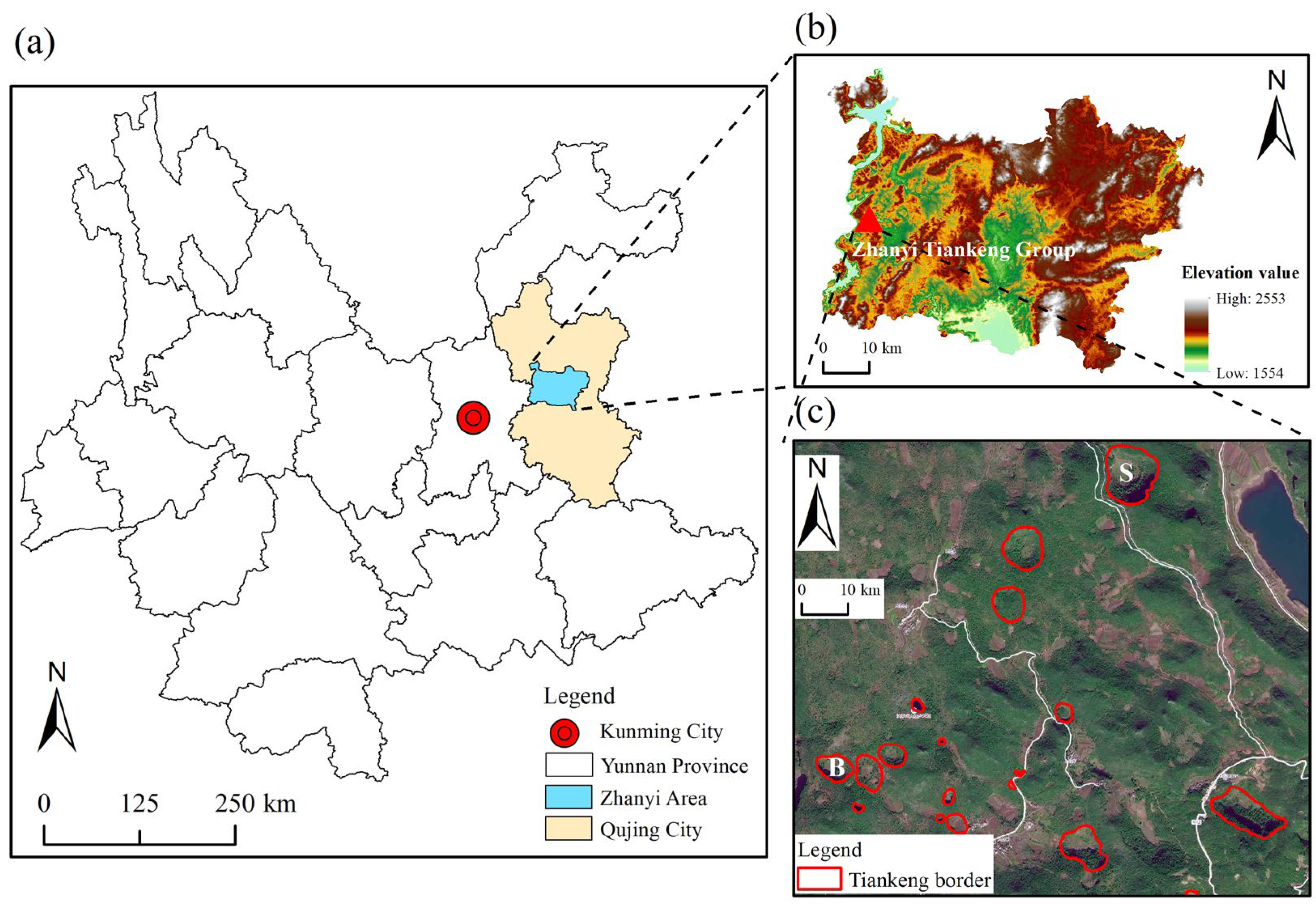
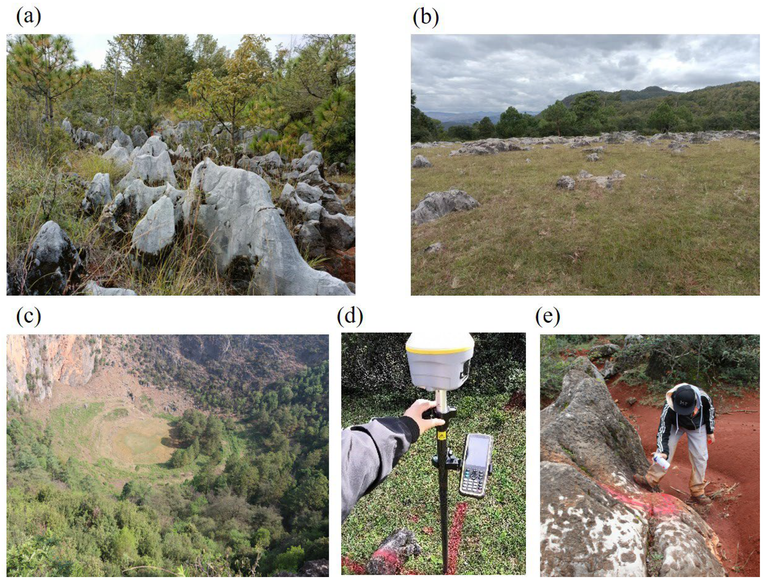
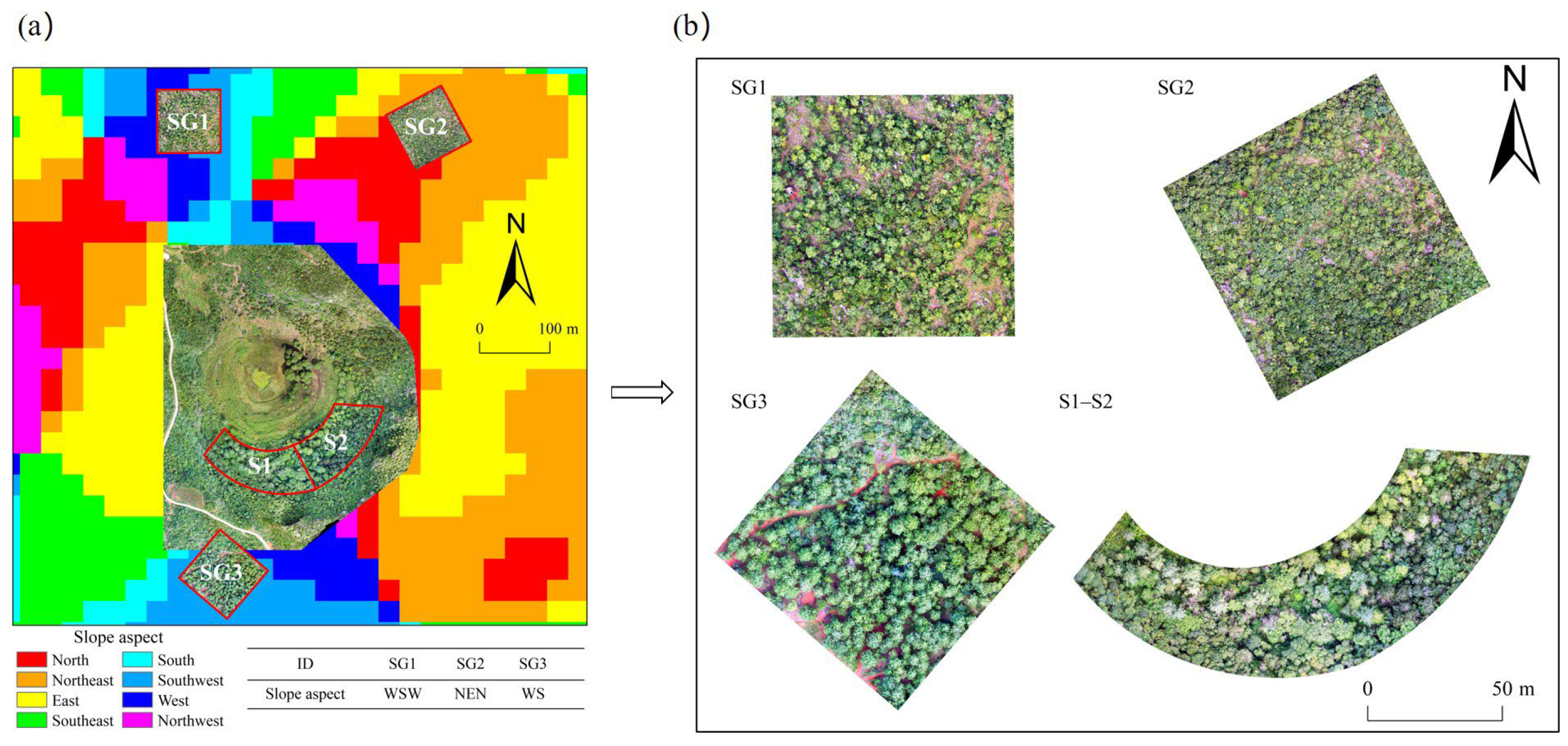
2.1. Study Area

We took the Zhanyi Tiankeng Group, located in Haifeng Nature Reserve, Yunnan Province (25°35′–25°57′N, 103°29′–103°39′E), as the study area. Here, primary and degraded tiankengs coexist with varying morphological sizes and degradation levels [Figure 1]. This area lies in the transition zone from a temperate plateau climate to a subtropical plateau monsoon climate, with an annual precipitation of 1073.5 mm–1089.7 mm. With the daily temperature difference but the annual temperature difference is relatively small. The annual average temperature is about 13.8 °C. The total annual solar radiation is 123.8 kcal·cm⁻².

Shenxiantang tiankeng was selected for this study on the basis of field investigations, which is a typical moderately degraded tiankeng in the Zhanyi Tiankeng Group. Its elevation is 2028 m. The long and short diameter are approximately 422 m and 349 m, respectively. The depth is approximately 149 m. The Shenxiantang tiankeng is a larger scale tiankeng with undegraded vertical walls and almost no vegetation on its western side. The eastern side is a semi-degraded rock wall, with vegetation mainly consisting of sparse trees and shrubs, and has the main access road to the bottom of the tiankeng, which was once used by local residents for farming, but is currently fallow. The south slope is a completely degraded rock walls where form an underground forest with rich vegetation types. Through field surveys of woody plants, we found 19 species of trees in the Shenxiantang tiankeng. The main tree types in the underground forests on the south side of Shenxiantang tiankeng are Pinus yunnanensis, Keteleeria evelyniana, Quercus variabilis, Alangium chinense, Cyclobalanopsis glauca, Cornus capitata, Quercus guyavifolia, Cornus oblonga, etc. Samples were randomly set up at areas with dense vegetation, good tree growth, and little difference in plant type and growth. We set up three samples on the tiankeng-outside, namely SG1–SG3. Other samples were set up in the tiankeng, namely S1 and S2 [Figure 2].

2.2. Data Collections

We chose the DJI (Da Jiang Innovations) Royal 2 Mavic Pro UAV, which is manufactured by China DJI Innovation Technology Co. The UAV weighs 907 g and possesses a 1/2.3-inch CMOS RGB image sensor with 12.35 million effective pixels. With a lightweight, and easy to carry, the aerial photos can be obtained in red, green and blue visible bands at a high definition.

The UVA missions were implemented from 11:00 to 12:30 on 4 October 2022. During the data acquisition period, the weather conditions were favorable, with adequate solar illumination, calm winds with breeze and no clouds cover. We chose the takeoff point in the open area outside the tiankengs after route planning [Figure A1 in Appendix A]. Using the DJI flight planner and Pix4DCapture apps to plan the flight missions. We set the flight height to 70 m above ground level. The front overlap and side overlap were set to 70% and 63%, respectively. The study area has a special topography, with a large elevation drop, and no signal inside. Therefore, the ground control points were obtained by RTK in the open area around the tiankeng-outside and marked with spray paint [Figure A1].

We collected auxiliary data such as DEM and vector boundary data of the study area. The DEM is a product of ASTER GDEM with a resolution of 30 m from the central geospatial data cloud platform (http://www.gscloud.cn accessed on 27 July 2022), which were used to determine the location (slope direction) of the sample outside the tiankeng. The slope direction of the study area was calculated by ArcGIS 10.5 software.

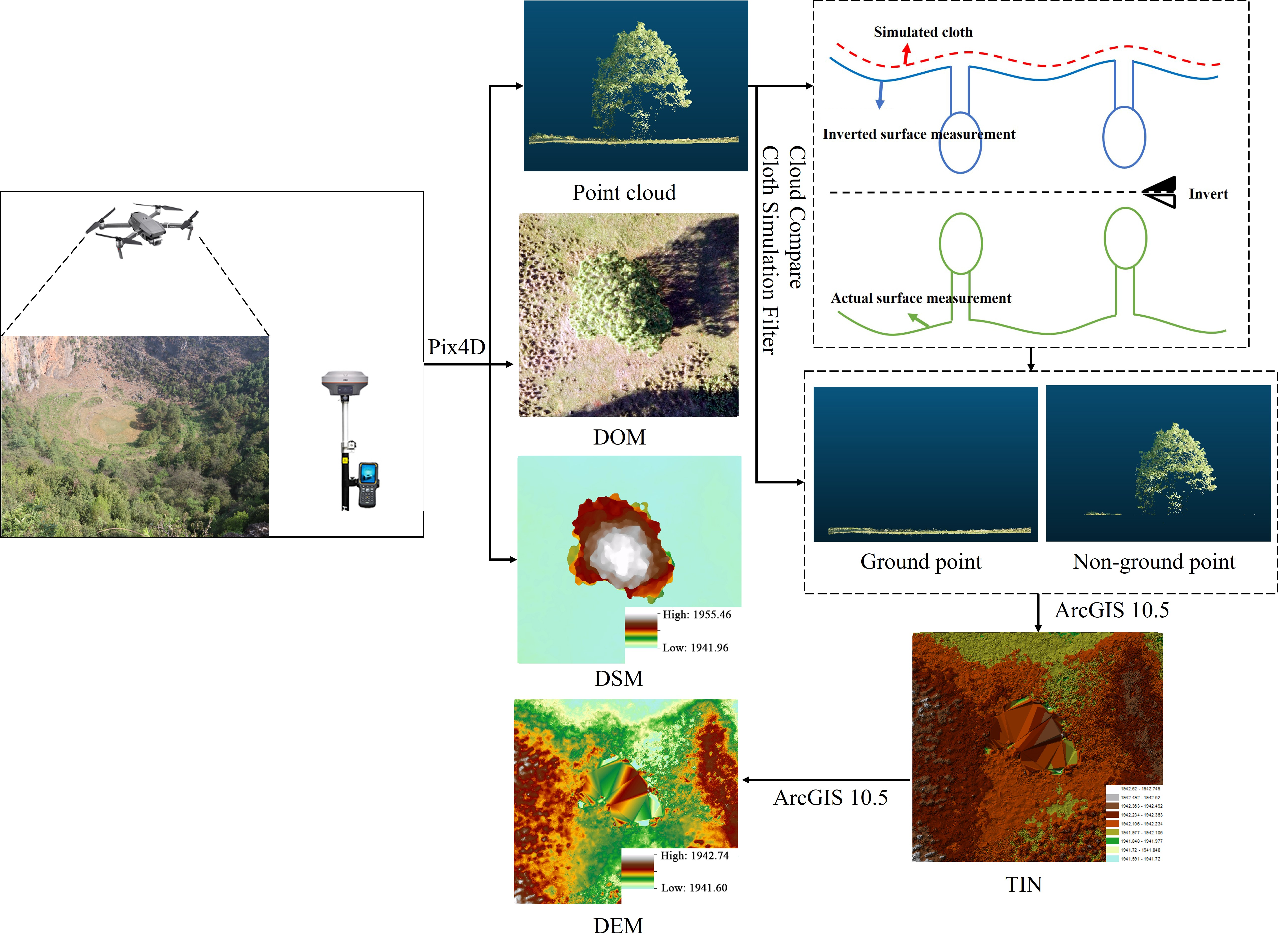
2.3. Data Processing

The UVA images were processed in the Pix4D mapper software. Firstly, we checked the photos and got 942 valid photos after deleting the photos with poor quality. Secondly, we imported the position information of the photos and ground control point in Pix4D mapper with the default WGS84 coordinates, followed by image adjustment, feature point matching, aerial triangulation, and image mosaic. Finally, the point cloud data (average point density 134.72 per m³), digital surface model (DSM) and digital orthophoto map (DOM) were obtained. After checking the quality report without error tips, we found no obvious seam lines and blurred features in the orthophoto image. This indicated that the experimental processing results meet the requirements of this study. The area of image covered is 860,000 m² and the ground sampling distance (GSD) of original images is 0.03 m. Taking into account the data processing efficiency and canopy extraction effect, we resampled all image data to 0.1 m. The original point clouds were separated into ground point clouds and canopy point clouds (non-ground points) using cloth simulation filter (CSF) algorithm in Cloud Compare software [23,35]. The non-ground points of other ground classes except the canopy point cloud were cleaned manually [23]. Cleaned ground point clouds were used to produce the Triangulated Irregular Network (TIN), and then converted to raster with a resolution of 0.1 m to obtain the DEM. Finally, the canopy height model (CHM) was obtained by subtracting the DSM from the DEM.

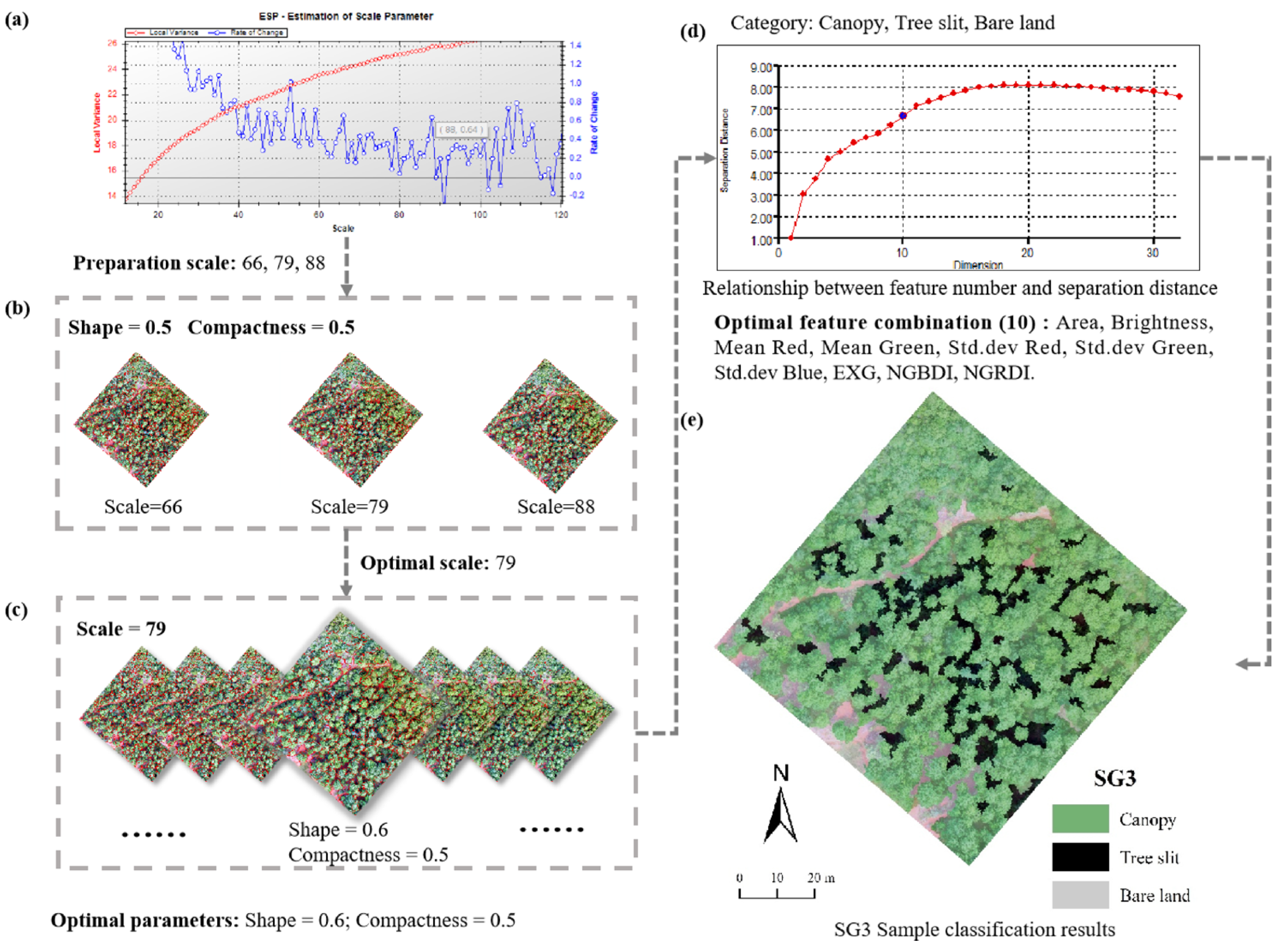
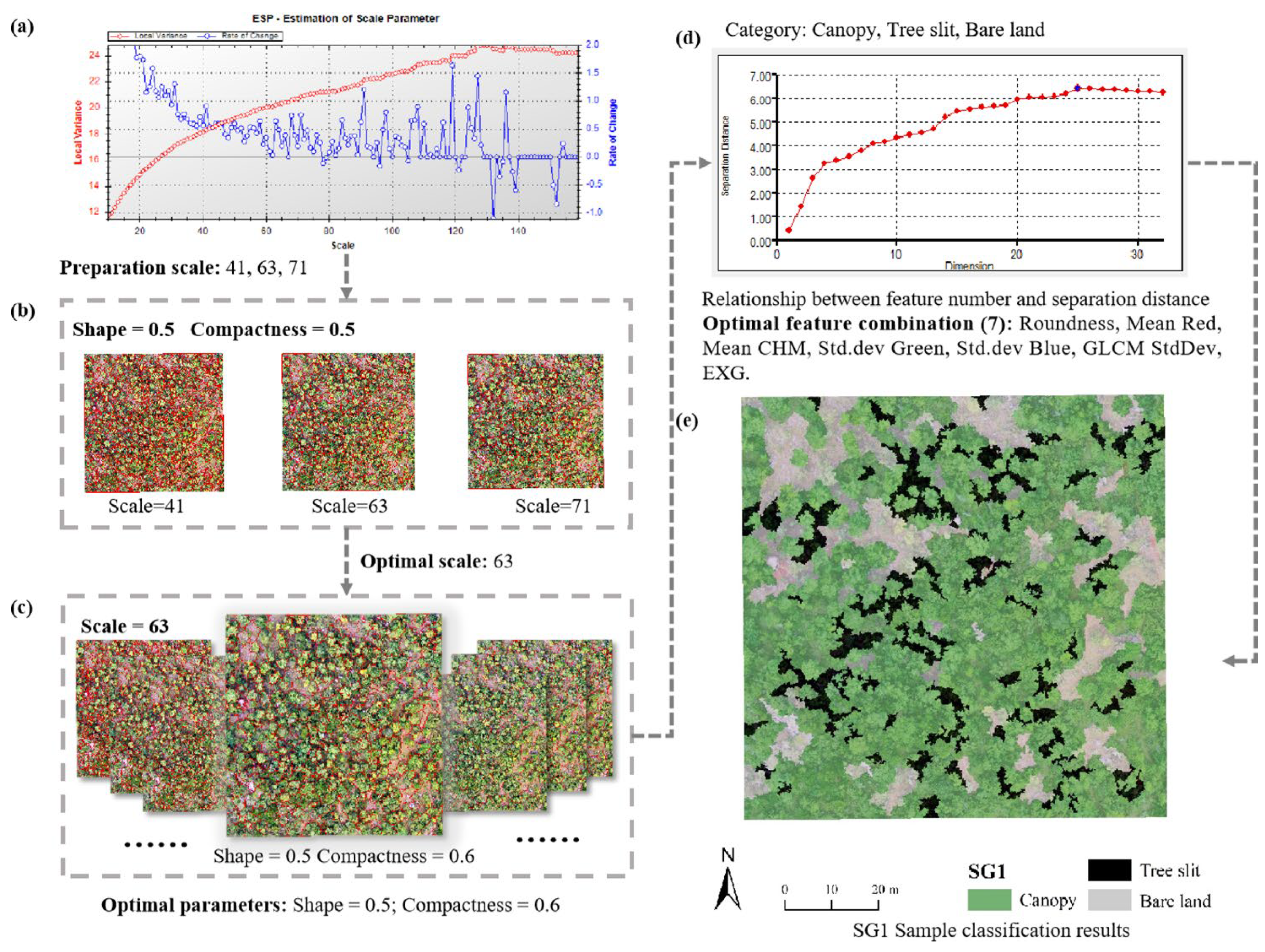
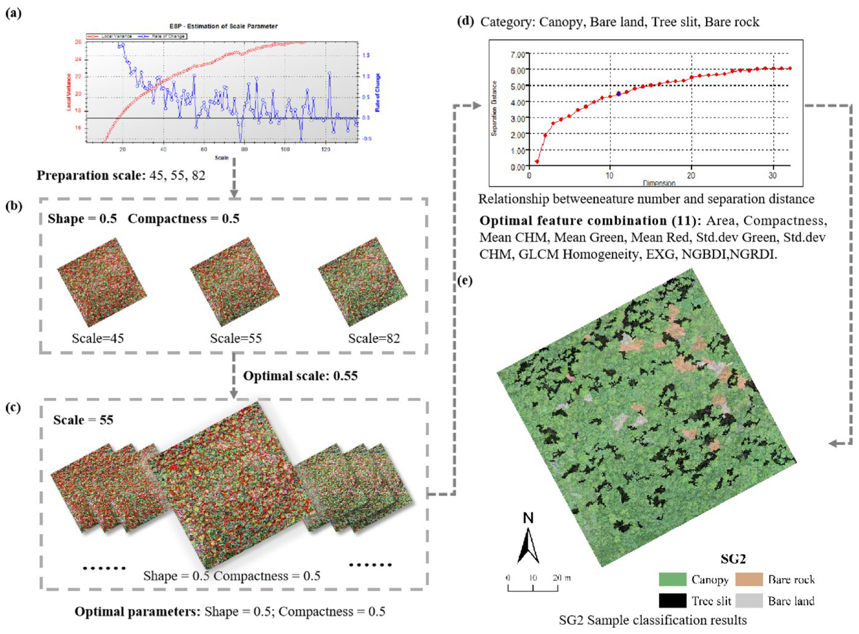
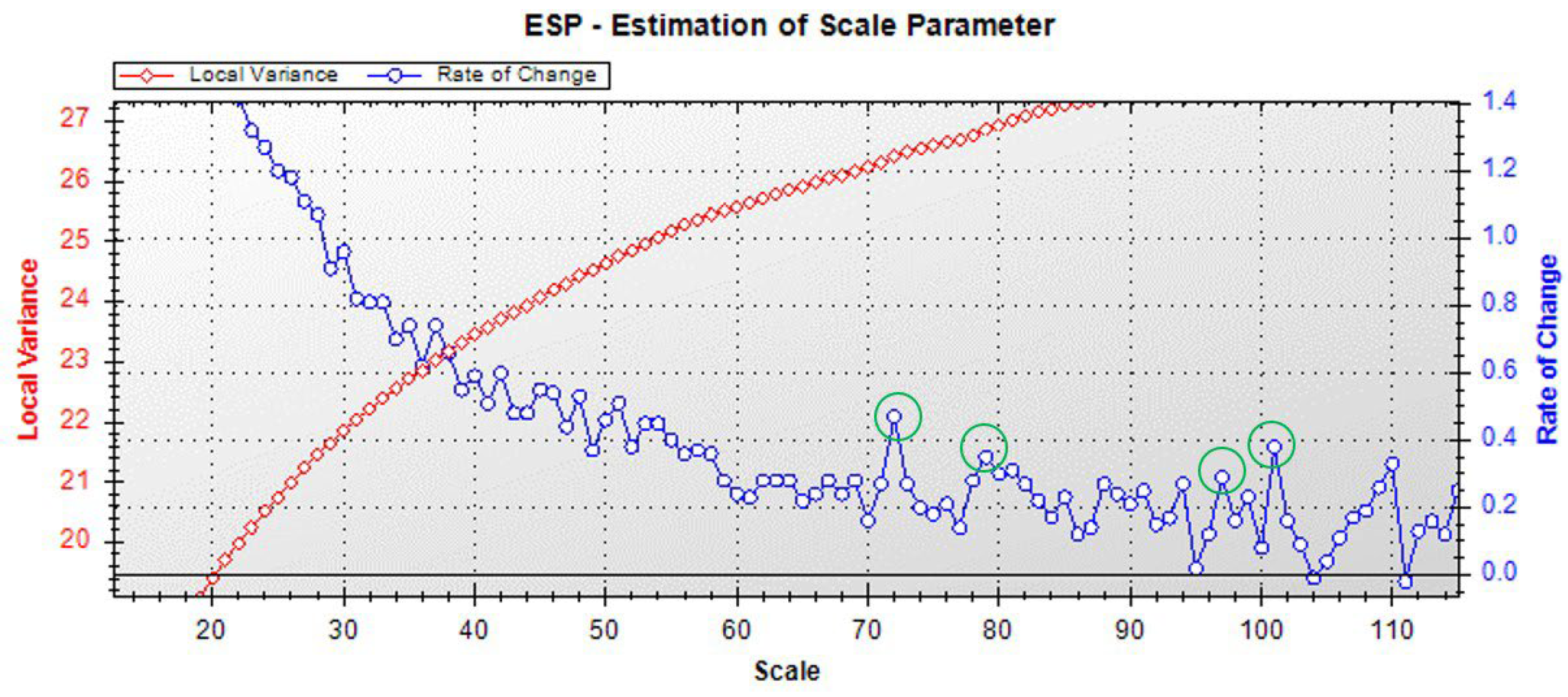
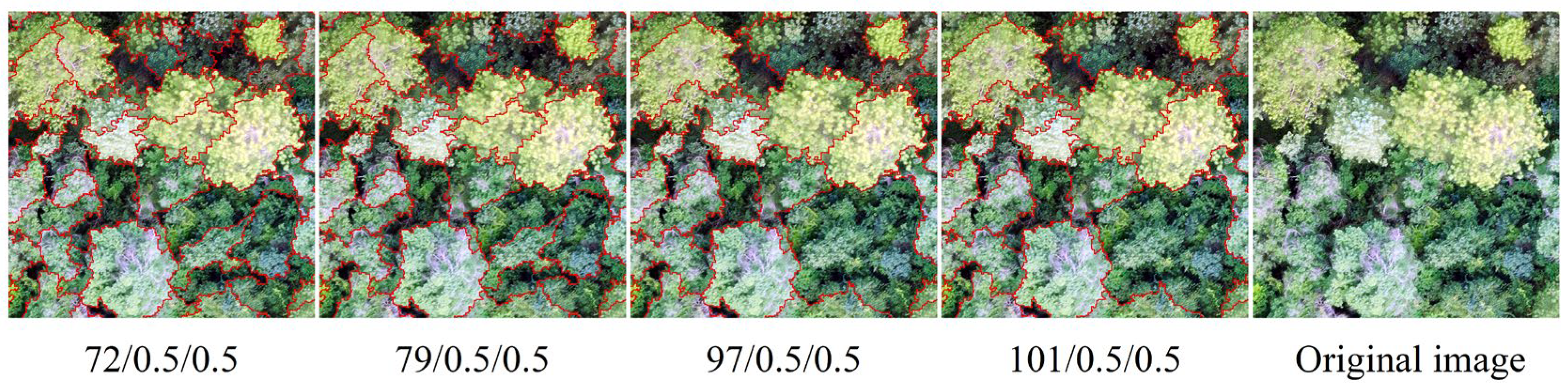
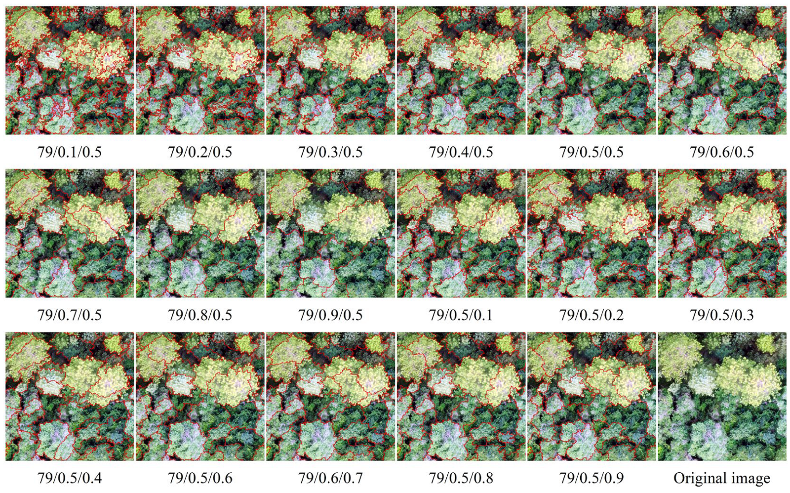
2.4. Multi-Scale Segmentation

To extract single wood canopies, we used the multi-scale segmentation algorithm in eCognition Developer from Definiens Imaging, Germany. Multi-scale image segmentation has been widely used in tree canopy extraction as a local optimization process. It is a top-down regional merging method that ensures minimum intra-object heterogeneity and maximum average object-to-object heterogeneity [36,37]. The scale parameter is an important parameter for multi-scale segmentation [38]. Other parameters that affect the segmentation results are shape parameters and compactness.

The optimal segmentation scale is estimated by using the Estimation of Scale Parameter (ESP) plug-in of the eCognition software. The ESP algorithm starts with a single pixel as an object and then iterates up the process species. Smaller image objects are merged to become larger image objects, and the minimized objects with internal homogeneity are obtained by continuous optimization [39]. The algorithm determines the best segmentation scale by calculating the rates of change (ROC) from the local variance (LV) of the image object [40]. When the ROC value is maximum, the segmentation scale corresponding to the peak presented is the optimal scale [27]. The shape and tightness parameters need to be tested repeatedly to obtain the best results. The optimal scale parameters are filtered by experiments comparing control variables using a multi-scale segmentation algorithm for optimal values of shape and tightness parameters. During the preliminary tests, we found that the optimal division scale ranged roughly from 10 to 200. Then we set the starting scale in the ESP plug-in to 10, the step size to 1, and the shape and tightness parameters to 0.5, with 200 cycles to finally obtain the segmentation parameter evaluation plots.

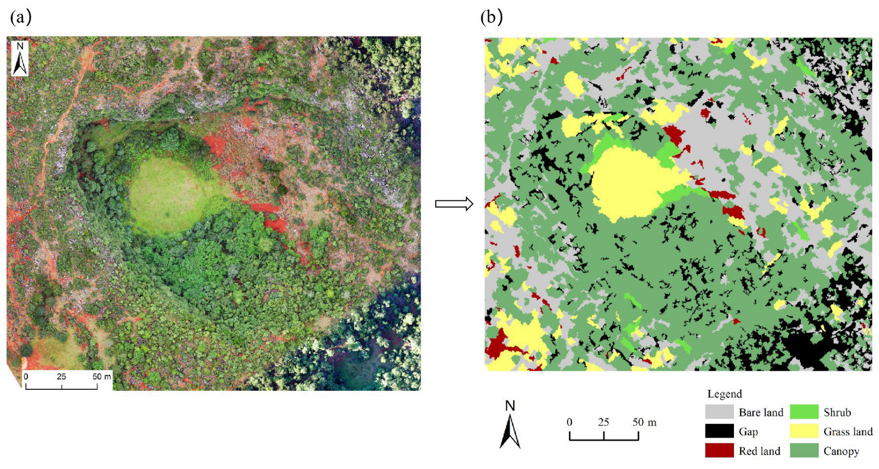
2.5. Object-Oriented Classification

The classification of object-oriented is mainly based on the different characteristics of objects. There are many object-oriented classification methods. However, the fuzzy classification method provided by eCognition software, which included two classifiers, the k-NN method and the membership function method [41,42]. We selected the k-NN classifier to extract canopy. The k-NN classifier compared each unknown sample directly to the original training data, without training to produce a model [43,44,45]. It is a simple and efficient non-parametric classification membership for they have obtained [46]. The method found the nearest neighboring sample object of each image object in the optimal feature space [47]. The principle consists of calculating the distance $d$ between each object to be classified and the sample object under the feature set, then to construct a multidimensional exponential affiliation function based on $d$ [48]. Finally, on the basis of the calculation result, the object to be divided belongs to the categories where its nearest sample objects are located. The equation for the feature space distance $d$ between the image object and the sample is as follows:

$$d=\sqrt{{\displaystyle \sum }_f{\left|\frac{v_f^s-v_f^o}{{\sigma }_f}\right|}^2}$$

(1)

where, $o$ is the image object; $s$ is the sample; $v_f^s$ is the eigenvalue of sample feature $f$; $v_f^o$ means the eigenvalue of object feature $f$; ${\sigma }_f$ means the standard deviation of sample feature $f$.

In the eCognition software, the classification of the image by the k-NN classifier depends on the degree of membership. The smaller the distance between the image object and the sample object, the greater will be the membership degree between that object and its class to which the sample belongs. The k-NN classifier using the eCognition software method performs classification as follows. Firstly, according to selected object features, we determined the classification system of the features, and collected the object features, as well as constructed the optimal feature space set using Feature Space Optimization tool. Then, the training sample for each feature was selected and the optimal feature space set was applied to refine the sample for classification. It requires a certain number of samples for each class of features, and the selection of training samples has a large impact on the classification results [31,49]. The k-NN is a supervised classification. A small number of training samples with distinctive features were selected by visual interpretation. Then, we considered whether to add training samples according to the classification effect. The classification should be performed by setting the affiliation threshold of the feature object and selecting the appropriate membership function. Finally, based on the feature space distance between the image and the sample object, the k-NN classifier will return the affiliation value. If the membership value outweighs the set threshold, the object is classified to the feature class to which the corresponding sample belongs. The k-NN classification method will be suitable for the classification of multiple object features.

2.6. Features Collection

Classification based on spectral information alone cannot be effective, as the low spectral resolution of UAV images, which may even cause different features with the same spectral properties to be incorrectly grouped together. Therefore, an alternative selection of other characteristic indices to participate in the calculation is needed to better distinguish between different features [50]. The feature set for the k-NN classification generally includes spectral, textures, shapes, custom indices, etc. However, getting more accurate classification with more features is not possible. Conversely, an increase in computational effort, or even decrease in classification accuracy might arise. Therefore, a feature space optimization tool will be used to construct the optimal set. The optimal feature combinations the feature combinations represented by the maximum value selected from the average minimum distance between two classes of the selected classes calculated in each feature space [51].

Our object-oriented feature space set consists of 32 features involving five aspects: vegetation indices, spectral features, shape features, texture features, and canopy height features.

2.6.1. Vegetation Index Characteristics

To obtain better extraction results, the following six vegetation indices were used to characterize the feature space set of vegetation indices: EXG, NGBDI, NGRDI, RGBRI, RGRI and VDVI (

Table 1. A feature space set of vegetation index characteristics.

Vegetation Index	Description
Excess green [52,53]	$EXG=2G-R-B$
Normalized green-blue difference index [52,54]	$NGBDI=\left(G-B\right)/\left(G+B\right)$
Normalized green-red difference index [54,55]	$NGRDI=\left(G-R\right)/\left(G+R\right)$
Red-green-blue ratio index [56]	$RGBRI=\left(R+B\right)/2G$
Red-green ratio index [57,58]	$RGRI=R/G$
Visible-band difference vegetation index [59]	$VDVI=\left(2G-R-B\right)/\left(2G+R+B\right)$

Note: Where R, G and B represent the red, green and blue bands, respectively.

).

2.6.2. Spectral Characteristics

In this study, the spectral features were selected from the mean, standard deviation (std. dev), brightness and maximum difference (max. diff) of the 3 visible band components of the remote sensing image: red, green, and blue. Eight spectral features were specifically selected as follows: mean red, mean green, mean blue, brightness, max. diff, std. dev. Red, std. dev. Green and std. dev. Blue. Its calculation formulas were as follows (

Table 2. A feature space set of spectral index characteristics.

Spectral Characteristics	Description	Explanation
Mean	$\overline{C_L}=\frac{1}{n}{\displaystyle \sum _{i=1}^n}{C}_{Li}$	The mean $\left(\overline{C_L}\right)$ is calculated from values $(C_{Li}$) of all n pixels that make up an image object.
Brightness	$b=\frac{1}{n_L}{\displaystyle \sum _{i=1}^{n_L}}\overline{C_L}$	The number of the image object divided by the sum of the mean values that containing spectral information (a mean of the spectral means of the image object).
Std. dev	$C_L=\sqrt{\frac{1}{n-1}{\displaystyle \sum _{i=1}^n}{\left(C_{Li}-\overline{C_L}\right)}^2}$	Standard deviation was calculated from all n pixels values that make up an image object.
Max. diff	$\Delta C_L=\overline{C_{L.Object}}-\overline{C_{L.SO}}$	The maximum difference between the mean of the Lth layer of an image object $(\overline{C_{L.Object})}$ and the mean of the Lth layer of the super object $(\overline{C_{L.SO}}$).

).

2.6.3. Shape Feature

The shape features reflected the aggregate characteristics of the image objects. The canopy had more obvious shape characteristics than other features. Guided by the actual situation, the following eight shape features were selected (

Table 3. An equation and explanation for the shape feature.

Shape Feature	Description	Explanation
Area	$S$	For georeferenced object, the area is equal to the number of pixels multiplied by the area value of each raster pixel; for object without a reference system, the area is the number of pixels contained.
Border length	$B=B_0+B_1$	The sum of the boundary of the image object.
Length/Width	$\gamma =\left[a^2+b^2\left(1-f\right)\right]/S$	The ratio of the length of the image object to the width. The index indicates the narrowness of the object.
Width	$W$	The width of image object.
Border index	$BI=B/2\left(L+W\right)$	The border length is twice the sum of the upper length and width. The index reflects the complexity of the object’s boundaries. An object is more irregular, the larger the value of the boundary index.
Compactness	$Com=C/\sqrt{S}$	The index measures the degree of fullness of the image object. Compactness increases the closer the image object is to a square shape.
Roundness	$Rou=4\pi S/C^2$	The index indicates the degree to which the image object is close to circular.
Shape index	$A=C/4\sqrt{S}$	Describe the degree of smoothness of the image object boundary. The larger the index, the more broken the boundary; conversely, the smoother the boundary.

Note: $S$ is the area of the image object. $B$ is the boundary length, and $B_0$ and $B_1$ are the inner and outer boundaries of the image object, respectively. $\gamma$ is the aspect ratio. $a,b$ are the length and width of the smallest outer rectangle of the image object, and $f$ denotes the weight. $W$ is the width of the image object. $BI$ is the boundary index and $L$ is the length of the image object. $Com$ means the compactness and $C$ means the circumference of the image object. $Rou$ represents the roundness of the image object. $A$ is the shape index of the image object.

).

2.6.4. Texture Characteristics

The texture features are obtained based on the pixel calculation. We noticed that there are smaller studies about the texture features of objects in the absolute sense. Considerable studies have shown that the analysis of texture features is mostly based on the Gray-Level Co-occurrence Matrix (GLCM), and domestic scholars have experimentally demonstrated that GLCM worked better [60,61,62]. We employed 8 well-known texture features, as shown in

Table 4. An equation and explanation for the texture features.

Texture Features	Formula	Description
Homogeneity	$Homogeneity={\displaystyle \sum _{i=0}^{n-1}}{\displaystyle \sum _{j=0}^{n-1}}p\left(i,j\right)/\left[1+{\left(i-j\right)}^2\right]$	Description of the homogeneity of the image. As image element values in GLCM are clustered on the diagonal, the greater the homogeneity of the image and the higher the homogeneity.
Contrast	$Contrast={\displaystyle \sum _{i=0}^{n-1}}{\displaystyle \sum _{j=0}^{n-1}}p\left(i,j\right){\left(i-j\right)}^2$	Reflects the depth of the image texture grooves and the clarity of the image. As the texture grooves are shallower, the contrast value is smaller, and the clarity of the corresponding image decreases; conversely, the contrast is large and the clarity is higher.
Dissimilarity	$Dissimilarity={\displaystyle \sum _{i=0}^{n-1}}{\displaystyle \sum _{j=0}^{n-1}}p\left(i,j\right)\left|i-j\right|$	Similar to contrast. Reflect the degree of difference of the object. As the value of dissimilarity is larger, the greater the change in regional contrast indicated by the value.
Entropy	$Entropy=-{\displaystyle \sum _{i=0}^{n-1}}{\displaystyle \sum _{j=0}^{n-1}}p\left(i,j\right)\left(log p\left(i,j\right)\right)$	Measurement the complexity of texture in the image object. As the texture in the image becomes more complex, the entropy value increases; conversely, the entropy value decreases.
ASM	$ASM={\displaystyle \sum _{i=0}^{n=1}}{\displaystyle \sum _{j=0}^{n-1}}{\left(p\left(i,j\right)\right)}^2$	Represents the homogeneity and consistency of image grayscale distribution. The object distribution is concentrated near the main diagonal, and the image grayscale distribution is more uniform in the local area, and the ASM value is larger. On the contrary, if all values of the matrix are equal, the ASM value is smaller.
Mean	$Mean={\displaystyle \sum _{i=0}^{n-1}}{\displaystyle \sum _{j=0}^{n-1}}i\times p\left(i,j\right)$	Reflect the degree of image texture regularity. As the mean value is larger, the regularity of the texture is stronger, and the texture features are easier to describe; conversely, the texture is more difficult to describe.
Std. dev	$Std.dev=\sqrt{{\left(i-Mean\right)}^2{\displaystyle \sum _{i=0}^{n-1}}{\displaystyle \sum _{j=0}^{n-1}}p\left(i,j\right)}$	Reflect the degree of deviation that occurs between the image element value and the mean value. The standard deviation increase becomes greater as the image grayscale value becomes larger.
Correlation	$Correlation={\displaystyle \sum _{i=0}^{n-1}}{\displaystyle \sum _{j=0}^{n-1}}p\left(i,j\right)\left(i-{\mu }_i\right)\left(j-{\mu }_j\right)/\sqrt{\left({\sigma }_i{}^2\right)\left({\sigma }_j{}^2\right)}$	Measurement the similarity of image element values in the row or column direction, reflecting the local grayscale correlation in the image. Correlation values are larger when the values of matrix elements are close to uniformly equal; conversely, smaller.

.

2.6.5. Canopy Height Feature

CHM is a model that reflects the vertical distance between the tree canopy and the ground. It helped to differentiate the tree canopy from other ground cover types. This study chose 2 canopy height features: mean CHM and std. dev.CHM.

2.7. Extraction Method of Forest Structure Parameters

2.7.1. Canopy Density

Canopy density was calculated by dividing the area of canopy types in the classification results by the total area of the sample plots. We obtained the reference value of canopy density using the sample line method. Such a method for canopy density measurement is considered as the most reliable among the methods comparing with the results of remote sensing image-based crown density estimation [63,64]. We used the orthophoto of the UAV as background image, with the sample lines laid on the diagonal and median lines (Figure A2). Then, the total length of the canopy on the measurement lines was measured along the direction of the measurement lines. Next, each canopy densities on each line were obtained by taking the ratio of the canopy length on each measurement line to the measurement line. Finally, the average crown density of the four sample lines was considered as the crown density of the sample sites. The calculation formulas are as follows:

$$P_i=\frac{l_i}{L_i}$$

(2)

$$P=\frac{1}{n}{\displaystyle \sum }_{i=1}^n{P}_i$$

(3)

where: $l_i$ is the sum of the canopy lengths on a given line, $L_i$ is the total length of a given line, n is the number of lines, and $P_i$ is the ratio of the canopy length to the total line length along a given line.

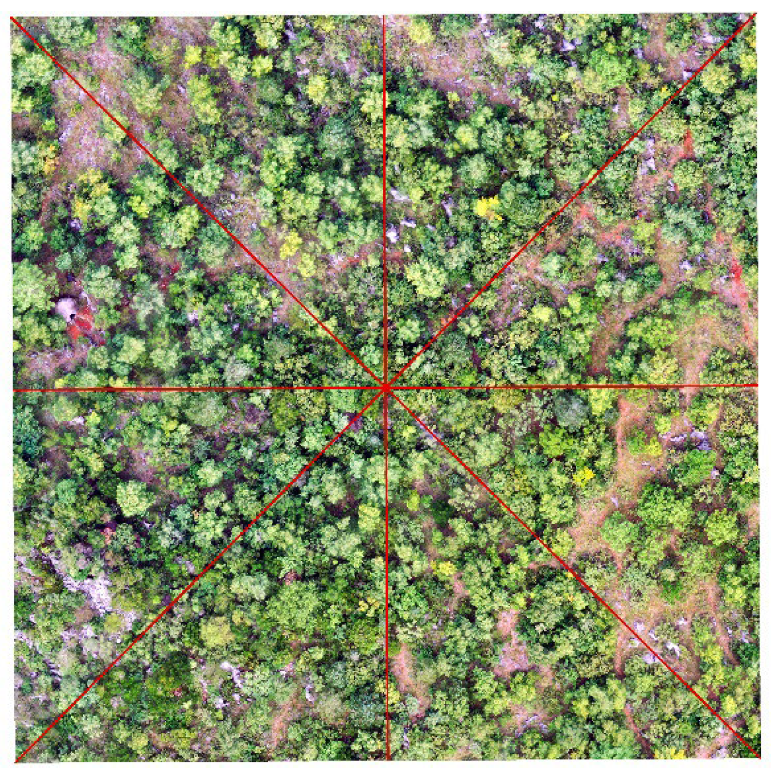
2.7.2. Average Crown Width

The crown width is the average width of trees in the north-south and east-west directions. Li et al. [63] considered the crown width as circular and got better results by calculating the average crown width ($\overline{P}$) from the canopy object area via the circular equation. This method provided a way to calculate the canopy size inside and outside the tiankengs. The calculation equation was as follows:

$$\overline{P}=2\sqrt{S/\pi }$$

(4)

where, S is the area of each object. The reference value of the crown width is obtained using the visual interpretation results.

2.8. Precision Verification

In this paper, the confusion matrix (overall accuracy, producer’s accuracy, and user’s accuracy) and kappa coefficients were used to accuracy verification [65]. The kappa coefficient is a statistical measure of inter-rater agreement or inter-annotator agreement for qualitative (categorical) items. The kappa coefficient can objectively evaluate the classification quality. Larger values of kappa coefficient indicate higher classification accuracy. In this study, 1500 random validation samples were initially setup to determine their categories by visual interpretation, and then the classification results of each sample point were obtained by the identity tool in ArcGIS10.5 to evaluate the accuracy of the classification results.

The stand parameters include canopy densities and canopy widths. The accuracy of canopy density extraction was estimated by comparing the extraction results of sample line method and object-oriented method. Since the sample area of the tiankeng-inside is an irregular rectangle, the accuracy verification of canopy density extraction results focuses on the sample area of the tiankeng-outside. The accuracy of the canopy parameter was verified by comparing the extracted canopy area and the visual interpretation. The complex terrain of the tiankengs made it dangerous to carry out field ground surveys, while this measurement method enabled to overcome this problem and eliminated the errors caused by human factors [65,66].

3. Results

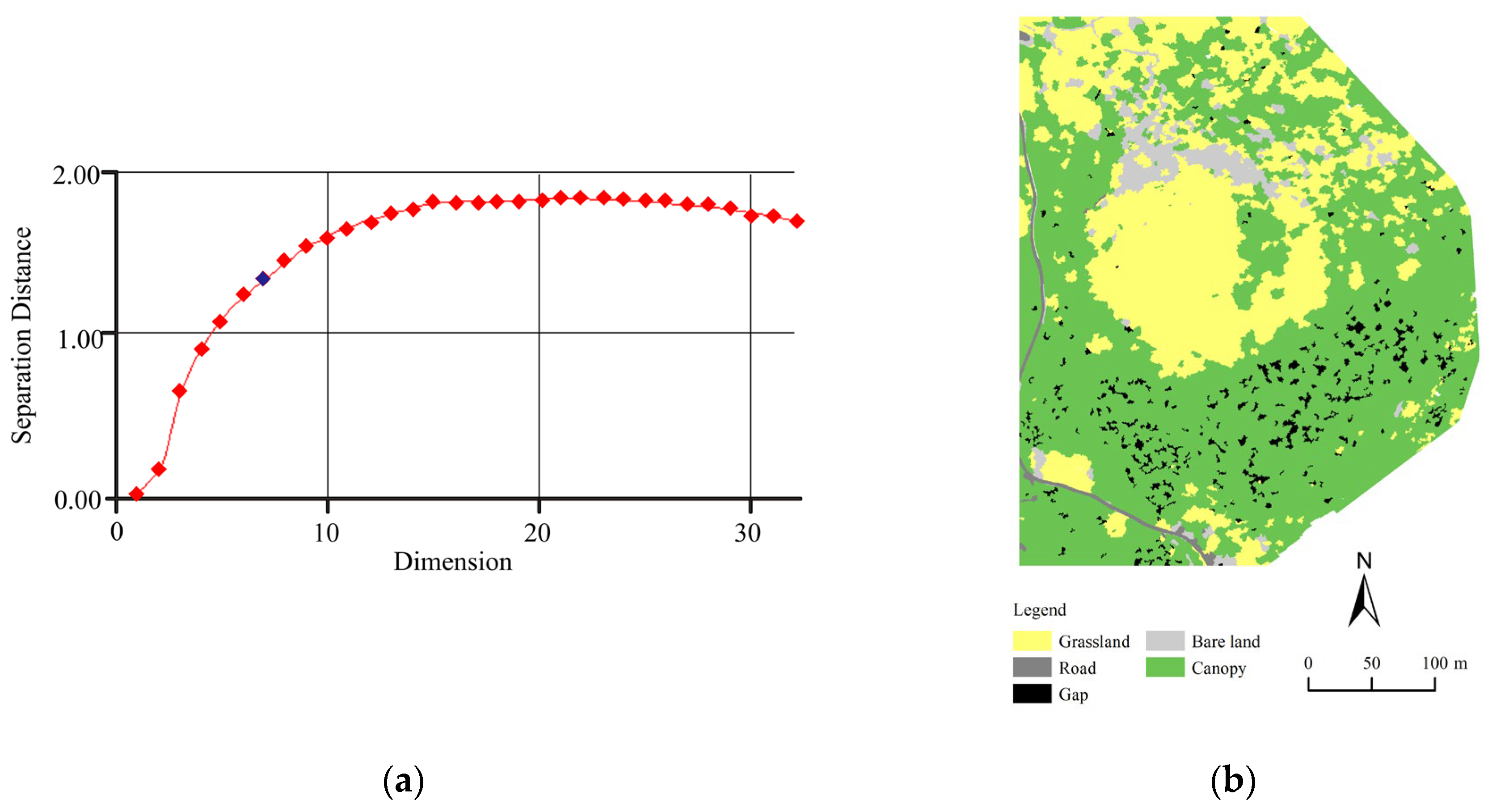
3.1. Canopy Extraction from Tiankengs

The alternative optimal segmentation scale parameters were 72, 79, 97, and 101 (Figure 3). Select default values for shape and compactness parameters to obtain visually correct segmentation results (Figure 4). Comparing the segmentation line with the original canopy shape on the image, we found when scale = 79, the edges of the tree canopy were well outlined. When the scale < 79, there was a case that a tree canopy was divided into multiple objects, and when the scale > 79, some of tree shadows were mixed with the canopy. Thus, the optimal segmentation scale parameter was determined to be 79. The best shape and compactness factors were then screened by comparison tests of control variables, which allowed for 17 sets of segmentation results (Figure 5). It was found that the best results were obtained when the shape parameter was set to 0.5 and the compactness to 0.8.

According to the actual situation, we classified the Shenxiantang tiankeng into five types: canopy, grass, road, tree gap and bare land. Then, we selected the training samples for feature selection, calculated the relationship between the number of features and the minimum feature distance between objects (Figure 6a). We found that when the number of features was 7, the objects were well differentiated, and the computation effort was appropriate. The optimal feature combination was NGBDI, GLCM Correlation, RGRI, area, std. dev CHM, std. dev Green, and std. dev Blue. The classification results based on the optimal feature combination using the nearest neighbor classifier are shown in Figure 6b.

Using the same method, we also extracted the canopy of another tiankeng (Bajiaxiantang) (Figure 7a). The best segmentation parameters were 63 (scale), 0.5 (shape), 0.2 (compactness). The land cover of classification results based on the optimal feature combination using the k-NN classifier were shown in Figure 7b. It was divided into six types: grass, shrub, red land, gap, canopy, and bare land. The training samples were selected for feature screening. The relationship between the number of features and the minimum feature distance between objects was calculated. We found that when the number of features was 7, each object had a good differentiation, and the computation was appropriate. The optimal combination of features was red, area, std. dev Green, std. dev CHM, EXG, NGBDI, length/width.

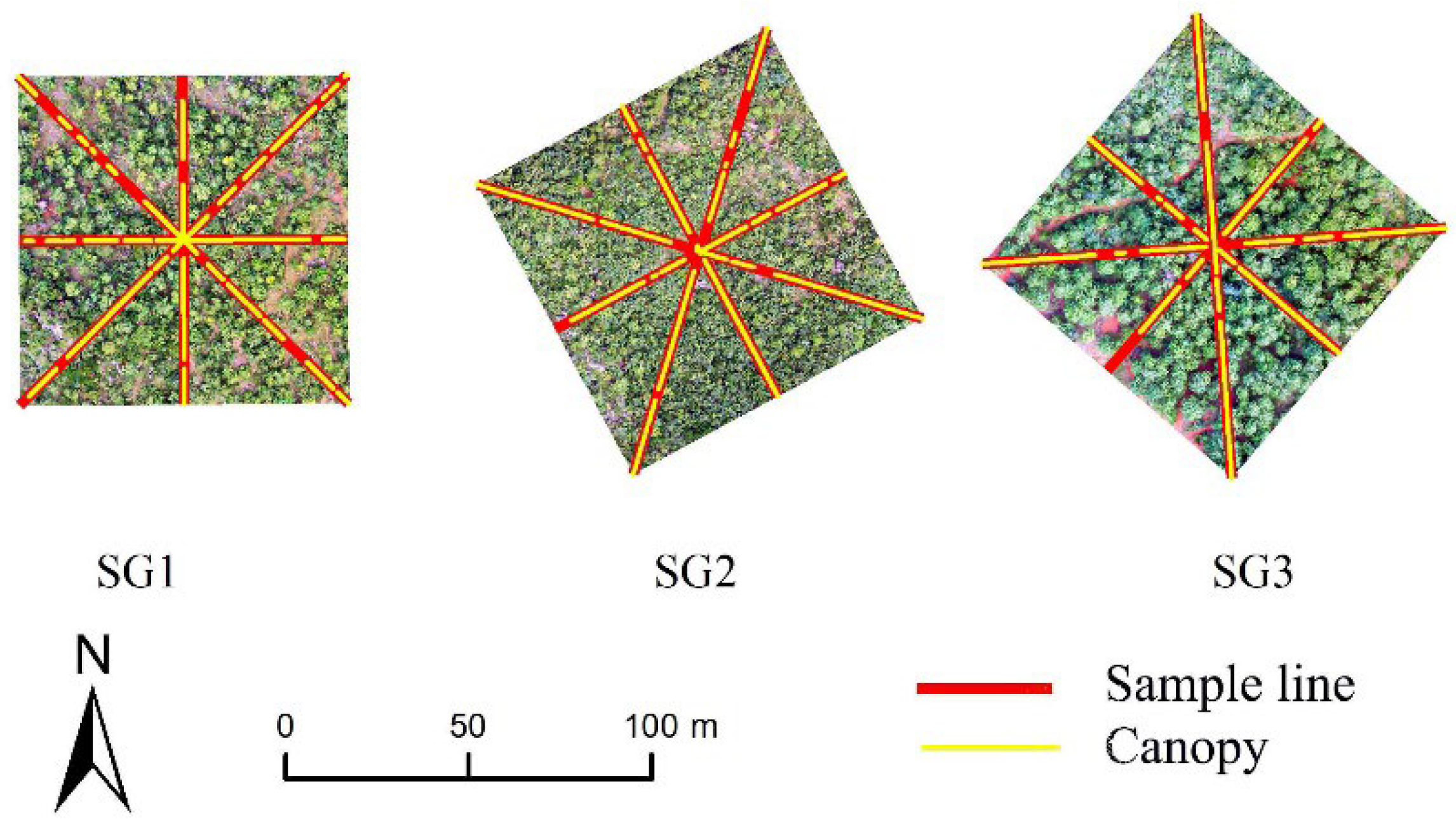
3.2. Canopy Extraction from the Ground Outside the Tiankeng

We combined the DOM and CHM data and used the object-oriented approach to extract the canopy information. The extraction results of the SG1–SG3 samples were shown in Figure A3, Figure A4 and Figure A5, and it could be seen that the canopy extraction is in general better. For samples SG1–SG3, we obtained alternative scales of 41, 63, 71 (SG1); 45, 55, 82 (SG2) and 66, 79, 88 (SG3), respectively, using the ESP2 tool for calculation. We also set the shape and compactness parameters to 0.5 for each of the three sample squares for comparison, and the best segmentation scales were obtained for each square as 63, 55 and 79. Then, we obtained the best segmentation effect by iterating through the shape and compactness parameters: 0.5/0.6; 0.5/0.5; 0.6/0.5, respectively. According to the actual situation of samples SG1–SG3, they were divided into four categories: canopy, tree slit, bare land and bare rock (among them, samples SG1 and SG3 had no bare rock), and the relationship between the number of features and separation distance was calculated to obtain the optimal combination of features for each sample (

Table A1. The area of each square classification results on the surface outside the Shenxiantang tiankeng.

Sample Code	Canopy (m2)	Tree Slit (m2)	Bare Land (m2)	Bare Rock (m2)
SG1	5640.8	906.3	1552.3	-
SG2	6545.9	1128.6	125.3	299.9
SG3	6404.6	1033.1	662.2	-

). We thus obtained the optimal feature combinations and canopy areas for each square as shown in

Table 5. An optimal combination of features for surface samples outside the Shenxiantang tiankeng.

Samples	Optimal Feature Combination	Canopy Area
SG1	Roundness, Mean Red, Mean CHM, Std. dev Green, Std. dev Blue, GLCM Std. dev, EXG	5640.87 (m2)
SG2	Area, Brightness, Mean Red, Mean Green, Std. dev Red, Std. dev Green, Std. dev Blue, EXG, NGBDI, NGRDI	6545.99 (m2)
SG3	Area, Compactness, Mean CHM, Mean Green, Mean Red, Std. dev Green, Std. dev CHM, GLCM Homogeneity, EXG, NGBDI, NGRDI	6404.66 (m2)

.

3.3. Extraction of Forest Stand Parameters

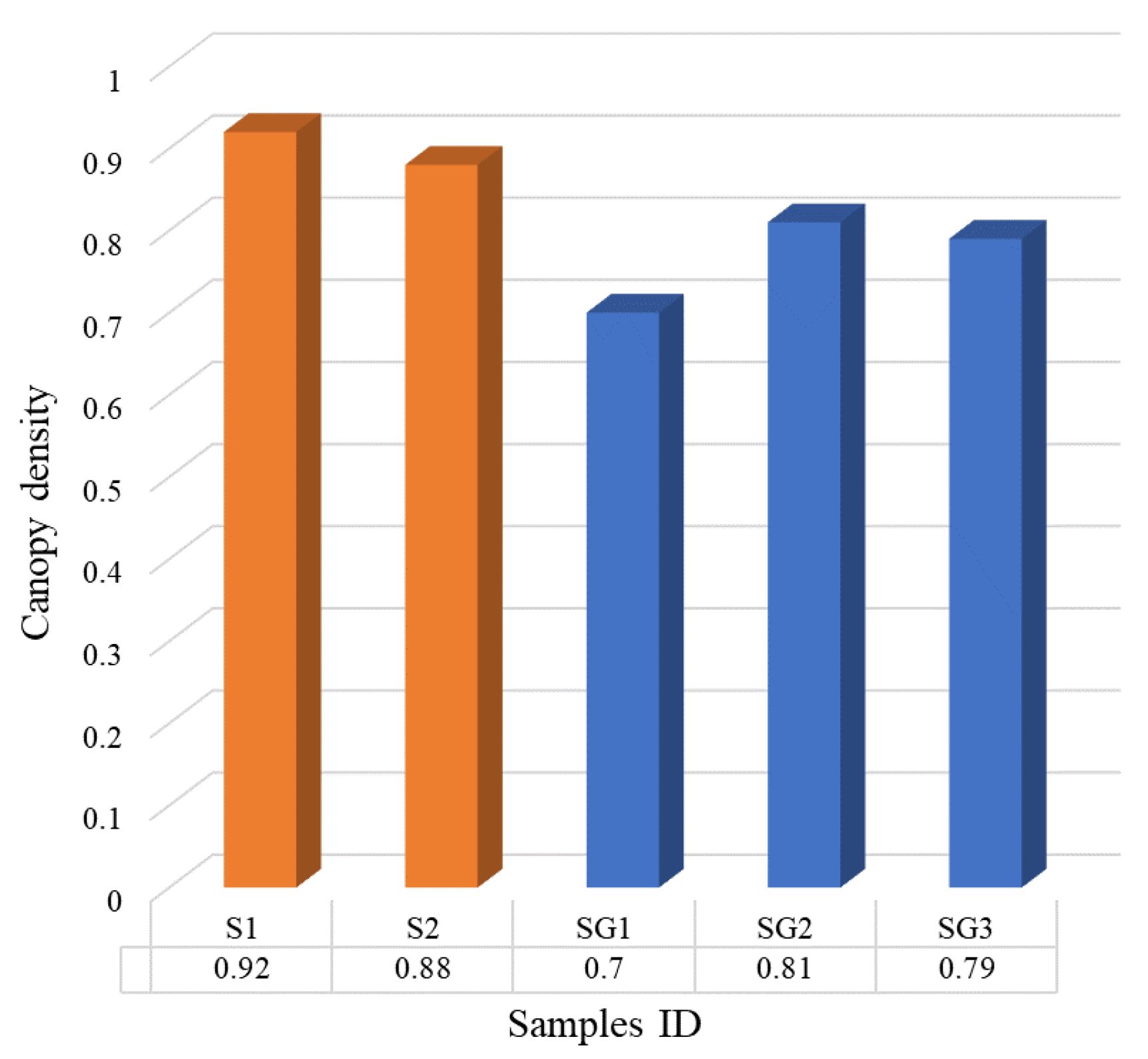
3.3.1. Forest Canopy Density

Based on the object-oriented canopy extraction results, we found two samples in the underground forest of tiankeng were dense forests. The canopy densities of samples S1, S2 inside the tiankeng were 0.92 and 0.88, respectively. Outside the tiankeng, all samples were dense forests, too. Overall, the canopy density in the underground forest was higher than the tiankeng-outside (Figure 8).

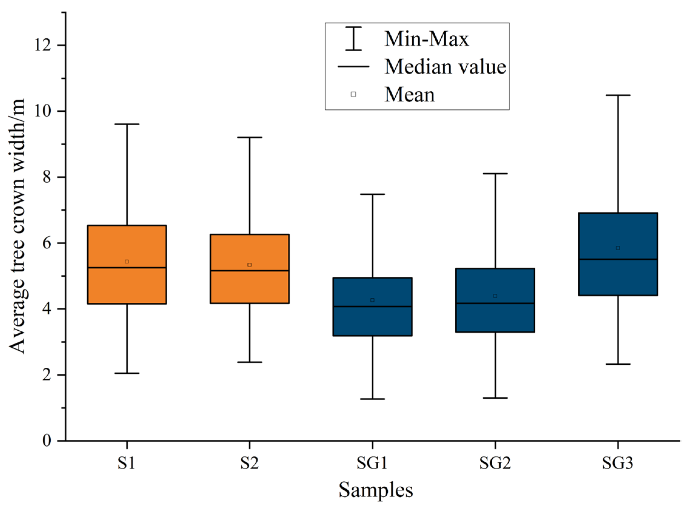
3.3.2. Average Crown Width

We found that the mean canopy width was 5.38 m inside the tiankeng samples and 4.83 m outside the tiankeng samples (Figure 9). The mean canopy width inside the tiankeng was significantly larger than that outside (p < 0.000). Some tree canopies were split into multiple objects by the object-oriented segmentation method. This reflected to some extent the fact that the trees in the underground forest inside the tiankeng had larger canopies than outside. We observed the canopy width of the samples inside the tiankeng was not much different.

3.4. Accuracy Verification Results

3.4.1. Classification Result Accuracy Verification

In this study, we took the Shenxiantang tiankeng as an example, generated 1500 points randomly within the Shenxiantang tiankeng as a validation sample. Using visual interpretation to classify the sample points for accuracy evaluation of the confusion matrix (

Table 6. An analysis of the accuracy of classification results of Shenxiantang tiankeng.

	Reference	Canopy	Bare Land	Grassland	Road	Tree Slit	Total	User Accuracy
Classification
Canopy		865	13	45	13	15	951	0.91
Bare land		9	40	11	0	0	60	0.67
Grassland		86	2	344	1	6	439	0.78
Road		1	0	0	10	0	11	0.91
Tree slit		8	0	0	0	31	39	0.79
Total		969	55	400	24	52	1500
Production accuracy		0.89	0.73	0.86	0.42	0.60
Overall accuracy = 85.6%; Kappa coefficient = 0.72

). We found that the overall classification accuracy was 85.60% and the kappa coefficient was 0.72. The extraction accuracy of canopy reached 0.91, which was better, and its main misclassification type was grass. Because, to a certain extent, the image features of canopy and grass had some similarities.

3.4.2. Accuracy Verification of Canopy Density Parameters

The areas of the canopy on the sample lines were marked in ArcGIS 10.5, as shown in Figure 10, and the lengths on each sample line were counted, as shown in

Table 7. An accuracy analysis of object-oriented method to extract sample plot canopy density.

Sample	Survey Line 1	Survey Line 2	Survey Line 3	Survey Line 4	Line Method to Extract Values	Object-Oriented Extraction of Values	Accuracy (%)
SG1	0.61	0.76	0.57	0.53	0.62	0.70	87.51%
SG2	0.84	0.68	0.54	0.62	0.67	0.81	79.53%
SG3	0.89	0.78	0.47	0.56	0.68	0.79	83.11%
Average	-	-	-	-	0.66	0.77	83.38%

. From the statistical results, the overall accuracy of the object-oriented canopy density extraction results was above 75%, with an average accuracy of 83.38%. The mean value of canopy density extraction by the line measurement method was 0.66, and the mean value of object-oriented extraction was 0.77. The overall result of object-oriented canopy density extraction was higher than the value extracted by the line measurement method, which was 0.1 higher on average. The object-oriented method also suffers from the wrong extraction of other classes as tree crowns. Although the study area is a complex karst topography, results of canopy parameters extraction are informative.

4. Discussion

4.1. Application Potential of UAV Technology in Tiankeng-like Underground Forests

The karst tiankeng topography is undulating, with large drop-offs inside and outside the tiankeng, and surrounded by vertical steep rock walls. Compared to other study areas, complexity of topography increased uncertainty of the canopy extraction results. Using high-resolution UAV remote sensing images as the data source and using the object-oriented classification method to better overcome these problems. UAV remote sensing images have very high spatial resolution and rich texture and shape features. Thus, the extraction results of the forest stand parameters based on UAV images better meet the practical demands [16,67,68,69].

Existing canopy extraction studies generally focus on plantation forests with small topographic differences and simple stand structure on positive topography [70,71]. Fewer studies have been conducted on special forests such as tiankeng underground forests. Constrained by the topographical factors of the tiankeng itself, the risk factor for carrying out large-scale forest surveys were high, and UAVs can overcome this obstacle. With the development of UAV technology, the quality of UAV aerial images has been improving. This study showed that UAVs provided reliable means of carrying out tiankeng underground forest research. The supportive argument was mainly in terms of the following two aspects. First, the classification accuracy of this study was better than the object-oriented classification results obtained in previous studies [16,72]. In tiankengs, the extraction results of canopy information had the highest accuracy relative to other classes. This is mainly due to the aggregation of forest tree growth and well-defined characteristics of underground tiankengs. The extraction accuracy of bare land and grassland was lower. Because the study focused on tree crowns, and hence the selection of parameters such as scale, shape and compactness were biased towards the applicability of the extraction effect on tree crowns. Therefore, the object features of bare land and grassland may not be more consistent. There was a small amount of grass in the object of bare land, and some tree canopies in the object of grass, which could cause some errors.

Second, UAVs could carry out deep-scale studies of tiankengs. Previous studies of tiankeng subterranean forests have been mostly conducted on tiankeng inverted stone slopes using sampling to study the characteristics of underground forests in vertical gradient, horizontal space, and other directions [9,73,74]. Although studies in these areas could provide some evidence to reveal the value of tiankengs as reservoir for species conservation, there are issues that cannot be addressed in this way. Therefore, we needed to obtain more comprehensive data from a global perspective to reveal its universal rules. Hence it was necessary and meaningful to use UAV technology to study tiankeng-like underground forests.

UAV remote sensing technology can promote the study of the plant functional trait ecology of karst tiankengs, but many issues remain to be further explored. Due to the special topography, the underground forest of the tiankeng is shaded by vertical cliffs, resulting in uneven lighting in the tiankeng. Thus, a way to obtain higher quality UAV images is also a research topic that we need to further explore in the future. We also need to obtain more bands of data and LIDAR data to study the stand parameters of tiankeng. Moreover, the poor accessibility of tiankengs made it difficult to acquire data in the field to verify the accuracy of the results. Finally, we further also need to use more object-oriented classification methods (random forests, support vector machines, single decision trees, artificial neural networks, etc.) to extract plant functional traits from the underground forest of karst tiankengs.

4.2. Feature Selection Is the Key to Tiankeng Underground Forest Canopy Extraction Based on UAV Images

Canopy parameters inside and outside the tiankengs can be expressed from the optimal combination of features for object-oriented classification, and different features express the information inside and outside the tiankeng to different ways. By counting the frequency of each feature being classified as the optimal feature combination. We found that the underground forest features NGBDI, std. dev Green, std. dev CHM and area contributed more to their classification in the tiankengs. While outside the tiankeng, the features EXG, mean Red, mean Green, Std. dev Green and area contributed more. As a whole, the area and green band features in the shape features play an important role in the classification of tiankengs and beyond. Shaded by the vertical cliffs of the tiankeng, the circled negative topography creates a local microclimate with a large heterogeneity and difference in habitat tiankeng-outside [6,7,75]. The inside of the tiankengs had higher air humidity, lower air temperature and higher concentration of negative oxygen ions [76,77]. This promoted the growth and reproduction of plants. The canopy and height of the trees inside the tiankengs were larger than outside [78]. The area of the tree canopy is more uniform and larger. Whereas the area of tree sutures is smaller, the area of bare ground is irregular. Therefore, the canopy can be well distinguished from other features by the area index.

In the vegetation index, NGBDI and EXG can better enhance the vegetation information and weaken the information of other features. Texture features contributed less to the identification of canopy information. Many textural features did not appear in the most characteristic combinations of all samples. This is consistent with the research results of Jin et al. [79]. They found that the accuracy of depression extraction was reduced by 0.66% owing to the addition of texture features. The canopy height CHM also played a larger role in the classification. It is an index of characteristics unique to trees. This indicated that the canopy height feature is an important parameter feature in forest canopy information [80,81]. This paper lacks consideration of terrain features in terms of feature collection, and terrain slope and roughness can also affect the extraction effect [82]. Non-remote sensing data such as slope, slope direction, roughness and environmental factors that have influence on plant growth are incorporated into the classification features. To summarize, a more suitable canopy classification feature set for negative terrain is the highlight of the next research work.

Comparing the canopy information extracted from inside and outside tiankengs. We found that the neighboring canopies in the underground forest tiankeng-inside often appear to cross each other and were distributed in clusters on the orthophoto. In this case, large errors would occur if traditional measurement methods were used. However, the image processing and analysis methods based on high-resolution UAV images not only use the information of individual pixels, but also make full use of the pixel information and image texture features to extract the single tree crowns in the form of images. So, the influence of the crossed tree crowns can be minimized, and the accuracy of the crown extraction can therefore be improved.

5. Conclusions

In this study, UAV visible images were combined with a canopy height model using an object-oriented multi-feature classification method to extract stand information such as canopy, canopy density and canopy width from the tiankeng underground forest and the tiankeng-outside. We therefore conclude the following:

(1)

UVA is a reliable technical tool to extract stand parameters in the underground forests of tiankeng. UAV could overcome the problem of inaccessibility of tiankengs. This helped to further explore the plant functional trait variability of underground forests of karst tiankengs. Drone technology has promoted plant ecology research.

(2)

The forest quality inside the tiankeng underground forest was better than those outside the tiankeng. The canopy density of the tiankeng was 0.90 and the average canopy width was 5.38 m. Outside the tiankeng, the canopy density and average crown width were 0.77 and 4.83 m, respectively. Compared with outside the tiankeng, the canopy density and canopy width of the underground forest were significantly larger. The enclosed tiankeng microhabitat provided a good habitat for plant communities.

References

1. Zhu, X.; Waltham, T. Tiankeng: Definition and description. Speleogenesis Evol. Karst Aquifers 2006, 1, 2. [Google Scholar]
2. Zhu, X.; Chen, W. Tiankengs in the karst of China. Carsologica Sin. 2006, 7–24. [Google Scholar] [CrossRef]
3. Zhu, X.; Zhu, D.; Huang, B.; Chen, W.; Zhang, Y.; Han, D. A brief study on karst tiankeng. Carsologica Sin. 2003, 22, 51–65. [Google Scholar]
4. Shui, W.; Chen, Y.; Wang, Y.; Su, Z.; Zhang, S. Origination, study progress and prospect of karst tiankeng research in China. Acta Geogr. Sin. 2015, 70, 431–446. [Google Scholar]
5. Shen, L.; Hou, M.; Xu, W.; Huang, Y.; Liang, S.; Zhang, Y.; Jiang, Z.; Chen, W. Research on flora of seed plants in Dashiwei Karst Tiankeng Group of Leye, Guangxi. Guihaia 2020, 40, 751–764. [Google Scholar]
6. Shui, W.; Chen, Y.; Jian, X.; Jiang, C.; Wang, Q.; Zeng, Y.; Zhu, S.; Guo, P.; Li, H. Original karst tiankeng with underground virgin forest as an inaccessible refugia originated from a degraded surface flora in Yunnan, China. Sci. Rep. 2022, 12, 9408. [Google Scholar] [CrossRef]
7. Pu, G.; Lv, Y.; Xu, G.; Zeng, D.; Huang, Y. Research progress on karst tiankeng ecosystems. Bot. Rev. 2017, 83, 5–37. [Google Scholar] [CrossRef]
8. Huang, L.; Yang, H.; An, X.; Yu, Y.; Yu, L.; Huang, G.; Liu, X.; Chen, M.; Xue, Y. Species abundance distributions patterns between tiankeng forests and nearby non-tiankeng forests in southwest China. Diversity 2022, 14, 64. [Google Scholar] [CrossRef]
9. Zhu, S.; Jiang, C.; Shui, W.; Guo, P.; Zhang, Y.; Feng, J.; Gao, C.; Bao, Y. Vertical distribution characteristics of plant community in shady slope of degraded tiankeng talus: A case study of Zhanyi Shenxiantang in Yunnan, China. Carsologica Sin. 2020, 31, 1496–1504. [Google Scholar]
10. Zang, R.; Jiang, Y. Review on the architecture of tropical trees. Sci. Silvae Sin. 1998, 5, 114–121. [Google Scholar]
11. Poorter, L.; Bongers, L.; Bongers, F. Architecture of 54 moist-forest tree species: Traits, trade-offs, and functional groups. Ecology 2006, 87, 1289–1301. [Google Scholar] [CrossRef]
12. Kohyama, T. Significance of architecture and allometry in saplings. Funct. Ecol. 1987, 1, 399–404. [Google Scholar] [CrossRef]
13. Tan, Y.; Shen, W.; Tian, H.; Fu, Z.; Ye, J.; Zheng, W.; Huang, S. Tree architecture variation of plant communities along altitude and impact factors in Maoer Mountain, Guangxi, China. Chin. J. Appl. Ecol. 2019, 30, 2614–2620. [Google Scholar]
14. Qin, X.; Li, Z.; Yi, H. Extraction method of tree crown using high-resolution satellite image. Remote Sens. Technol. Appl. 2005, 2, 228–232. [Google Scholar]
15. Wang, M.; Lin, J.; Lin, Y.; Li, Y. Subalpine coniferous forest crown information automatic extraction based on optical UAV remote sensing. For. Resour. Manag. 2017, 4, 82–88. [Google Scholar]
16. Sun, Z.; Pan, L.; Sun, Y. Extraction of tree crown parameters from high-density pure Chinese fir plantations based on UAV images. J. Beijing For. Univ. 2020, 42, 20–26. [Google Scholar]
17. Yan, L.; Liao, X.; Zhou, C.; Fan, B.; Gong, J.; Cui, P.; Zheng, Y.; Tan, X. The impact of UAV remote sensing technology on the industrial development of China: A review. J. Geo-Inf. Sci. 2019, 21, 476–495. [Google Scholar]
18. Zhu, X.; Meng, L.; Zhang, Y.; Weng, Q.; Morris, J. Tidal and meteorological influences on the growth of invasive spartina alterniflora: Evidence from UAV remote sensing. Remote Sens. 2019, 11, 1208. [Google Scholar] [CrossRef]
19. Chen, Y.; Hou, C.; Tang, Y.; Zhuang, J.; Lin, J.; He, Y.; Guo, Q.; Zhong, Z.; Lei, H.; Luo, S. Citrus tree segmentation from UAV images based on monocular machine vision in a natural orchard environment. Sensors 2019, 19, 5558. [Google Scholar] [CrossRef]
20. Yan, W.; Guan, H.; Cao, L.; Yu, Y.; Li, C.; Lu, J. A self-adaptive mean shift tree-segmentation method using UAV LiDAR data. Remote Sens. 2020, 12, 515. [Google Scholar] [CrossRef]
21. Wu, X.; Shen, X.; Cao, L.; Wang, G.; Cao, F. Assessment of individual tree detection and canopy cover estimation using Unmanned Aerial Vehicle based Light Detection and Ranging (UAV-LiDAR) data in planted forests. Remote Sens. 2019, 11, 908. [Google Scholar] [CrossRef]
22. Yan, D.; Liu, Z. Application of UAV-Based Multi-Angle hyperspectral remote sensing in fine vegetation classification. Remote Sens. 2019, 11, 2753. [Google Scholar] [CrossRef]
23. Avtar, R.; Suab, S.A.; Syukur, M.S.; Korom, A.; Umarhadi, D.A.; Yunus, A.P. Assessing the influence of UAV altitude on extracted biophysical parameters of Young Oil Palm. Remote Sens. 2020, 12, 3030. [Google Scholar] [CrossRef]
24. Chen, A.; Yang, X.; Xu, B.; Jin, Y.; Zhang, W.; Guo, J.; Xing, X.; Yang, D. Research on recognition methods of elm sparse forest based on object-based image analysis and deep learning. J. Geo-Inf. Sci. 2020, 22, 1897–1909. [Google Scholar]
25. Li, Q.; Liu, J.; Mi, X.; Yang, J.; Yu, T. Object-oriented crop classification for GF-6 WFV remote sensing images based on Convolutional Neural. Natl. Remote Sens. Bull. 2021, 25, 549–558. [Google Scholar]
26. Ma, F.; Xu, F.; Sun, C. Land-use information of object-oriented classification by UAV image. J. Appl. Sci. 2021, 39, 312–320. [Google Scholar]
27. Zhu, Y.; Zeng, Y.; Zhang, M. Extract of land use/cover information based on HJ satellites data and object-oriented classification. Trans. Chin. Soc. Agric. Eng. 2017, 33, 258–265. [Google Scholar]
28. Chang, C.; Zhao, G.; Wang, L.; Zhu, X.; Gao, Z. Land use classification based on RS object-oriented method in coastal spectral confusion region. Trans. Chin. Soc. Agric. Eng. 2012, 28, 226–231. [Google Scholar]
29. Sun, Z.; Shen, W.; Wei, B.; Liu, X.; Su, W.; Zhang, C.; Yang, J. Object-oriented land cover classification using HJ-1 remote sensing imagery. Sci. China Earth Sci. 2010, 53, 34–44. [Google Scholar] [CrossRef]
30. Zhang, S.; Wang, C.; Li, J.; Zhang, Z. An object-oriented and variogram based method of automatic extraction of tea planting area from high resolution remote sensing imagery. Remote Sens. Inf. 2021, 36, 126–136. [Google Scholar]
31. Liu, K.; Gong, H.; Cao, J.; Zhu, Y. Comparison of mangrove remote sensing classification based on multi-type UAV data. Trop. Geogr. 2019, 39, 492–501. [Google Scholar]
32. Pont, T.J.; Arbelaez, P.A.; Barron, J.; Marqués, A.F.; Malik, J. Multiscale combinatorial grouping for image segmentation and object proposal generation. IEEE T. Pattern Anal. 2017, 39, 128–140. [Google Scholar] [CrossRef] [PubMed]
33. Collins, M.J.; Dymond, C.; Johnson, E.A. Mapping subalpine forest types using networks of nearest neighbour classifiers. Int. J. Remote Sens. 2010, 25, 1701–1721. [Google Scholar] [CrossRef]
34. Han, N.; Du, H.; Zhou, G.; Sun, X.; Ge, H.; Xu, X. Object-based classification using SPOT-5 imagery for Moso bamboo forest mapping. Int. J. Remote Sens. 2014, 35, 1126–1142. [Google Scholar] [CrossRef]
35. Zhang, W.; Qi, J.; Wan, P.; Wang, H.; Xie, D.; Wang, X.; Yan, G. An easy-to-use airborne LiDAR data filtering method based on cloth simulation. Remote Sens. 2016, 8, 501. [Google Scholar] [CrossRef]
36. Benz, U.C.; Hofmann, P.; Willhauck, G.; Lingenfelder, I.; Heynen, M. Multi-resolution, object-oriented fuzzy analysis of remote sensing data for GIS-ready information. ISPRS J. Photogramm. 2004, 58, 239–258. [Google Scholar] [CrossRef]
37. Chen, Y.; Feng, T.; Shi, P.; Wang, J. Classification of remote sensing image based on object-oriented and class rules. Geomat. Inf. Sci. Wuhan Univ. 2006, 4, 316–320. [Google Scholar]
38. Su, W.; Li, J.; Chen, Y.; Zhang, J.; Hu, D.; Liu, C. Object-oriented urban land-cover classification of multi-scale image segmentation method-a case study in Kuala Lumpur city center, Malaysia. Natl. Remote Sens. Bull. 2007, 4, 521–530. [Google Scholar]
39. Ma, Y.; Ming, D.; Yang, H. Scale estimation of object-oriented image analysis based on spectral-spatial statistics. J. Remote Sens. 2017, 21, 566–578. [Google Scholar]
40. Dragut, L.; Tiede, D.; Levick, S.R. ESP: A tool to estimate scale parameter for multiresolution image segmentation of remotely sensed data. Int. J. Geogr. Inf. Sci. 2010, 24, 859–871. [Google Scholar] [CrossRef]
41. Dong, M.; Su, J.; Liu, G.; Yang, J.; Chen, X.; Tian, L.; Wang, M. Extraction of tobacco planting areas from UAV remote sensing imagery by object-oriented classification method. Sci. Surv. Mapp. 2014, 39, 87–90. [Google Scholar]
42. Liu, Y.; Yu, X.; Fan, J.; Zhou, J.; Cheng, H.; Yao, G.; Meng, F.; Jin, F. Rapid estimation of rural homestead area in Western China based on UVA imagery and object-oriented method. Bull. Surv. Mapp. 2022, 125–129. [Google Scholar] [CrossRef]
43. Altman, N.S. An introduction to kernel and nearest-neighbor nonparametric regression. Am. Stat. 1992, 46, 175–185. [Google Scholar]
44. Maxwell, A.E.; Warner, T.A.; Fang, F. Implementation of machine-learning classification in remote sensing: An applied review. Int. J. Remote Sens. 2018, 39, 2784–2817. [Google Scholar] [CrossRef]
45. Maselli, F.; Chirici, G.; Bottai, L.; Corona, P.; Marchetti, M. Estimation of mediterranean forest attributes by the application of k-NN procedures to multitemporal landsat ETM+Images. Int. J. Remote Sens. 2005, 26, 3781–3796. [Google Scholar] [CrossRef]
46. Wu, X.; Kumar, V.; Ross, Q.J.; Ghosh, J.; Yang, Q.; Motoda, H.; McLachlan, G.J.; Ng, A.; Liu, B.; Yu, P.; et al. Top 10 algorithms in data mining. Knowl. Inf. Syst. 2008, 14, 1–37. [Google Scholar] [CrossRef]
47. Zhang, Z.; Huang, Y.; Wang, H. A new KNN classification approach. Comput. Sci. 2008, 35, 170–172. [Google Scholar]
48. Mui, A.; He, Y.; Weng, Q. An object-based approach to delineate wetlands across landscapes of varied disturbance with high spatial resolution satellite imagery. ISPRS J. Photogramm. 2015, 109, 30–46. [Google Scholar] [CrossRef]
49. Zeng, Y.; Yang, Y.; Zhao, L. Pseudo nearest neighbor rule for pattern classification. Expert Syst. Appl. 2009, 36, 3587–3595. [Google Scholar] [CrossRef]
50. Zhang, Z.; Liu, W.; Li, X.; Zhu, J.; Zhang, H.; Yang, D.; Xu, X. The spatial distribution pattern of rock desertification area based on Unmanned Aerial Vehicle imagery and object-oriented classification method. J. Geo-Inf. Sci. 2020, 22, 2436–2444. [Google Scholar]
51. Huang, S.; Xu, W.; Xiong, Y.; Wu, C.; Dai, F.; Xu, H.; Wang, L.; Kou, W. Combining Textures and Spatial Features to Extract Tea Plantations Based on Object-Oriented Method by Using Multispectral Image. Spectrosc. Spect. Anal. 2021, 41, 2565–2571. [Google Scholar]
52. Woebbecke, D.M.; Meyer, G.E.; Von Bargen, K.; Mortensen, D.A. Color indices for weed identification under various soil, residue, and lighting conditions. Trans. ASAE 1995, 38, 259–269. [Google Scholar] [CrossRef]
53. Kazmi, W.; Garcia-Ruiz, F.J.; Nielsen, J.; Rasmussen, J.; Andersen, J.H. Detecting creeping thistle in sugar beet fields using vegetation indices. Comput. Electron. Agr. 2015, 112, 10–19. [Google Scholar] [CrossRef]
54. Woebbecke, D.M.; Meyer, G.E.; Bargen, K.V.; Mortensen, D.A. Plant species identification, size, and enumeration using machine vision techniques on near-binary images. Proc. SPIE-Int. Soc. Opt. Eng. 1993, 1836, 208–219. [Google Scholar]
55. Hunt, E.R.; Cavigelli, M.; Daughtry, C.S.T.; Mcmurtrey, J.E.; Walthall, C.L. Evaluation of digital photography from model aircraft for remote sensing of crop biomass and nitrogen status. Precis. Agric. 2005, 6, 359–378. [Google Scholar] [CrossRef]
56. Xie, B.; Yang, W.; Wang, F. A new estimation method for fractional vegetation cover based on UVA visual light spectrum. Sci. Surv. Mapp. 2020, 45, 72–77. [Google Scholar]
57. Verrelst, J.; Schaepman, M.E.; Koetz, B.; Kneubühler, M. Angular sensitivity analysis of vegetation indices derived from CHRIS/PROBA data. Remote Sens. Environ. 2008, 112, 2341–2353. [Google Scholar] [CrossRef]
58. Gamon, J.A.; Surfus, J.S. Assessing Leaf pigment content and activity with a reflectometer. New Phytol. 1999, 143, 105–117. [Google Scholar] [CrossRef]
59. Wang, X.; Wang, M.; Wang, S.; Wu, Y. Extraction of vegetation information from visible unmanned aerial vehicle images. Trans. Chin. Soc. Agric. Eng. 2015, 31, 152–159. [Google Scholar]
60. Kwak, G.H.; Park, N.W. Impact of texture information on crop classification with machine learning and UAV images. Appl. Sci. 2019, 9, 643. [Google Scholar] [CrossRef]
61. Castro, A.; Peña, J.; Torres-Sánchez, J.; Jiménez-Brenes, F.; López-Granados, F. Mapping cynodon dactylon infesting cover crops with an automatic decision tree-OBIA procedure and UAV imagery for precision viticulture. Remote Sens. 2019, 12, 56. [Google Scholar] [CrossRef]
62. Ojala, T.; Pietikainen, M.; Maenpaa, T. Multiresolution gray-scale and rotation invariant texture classification with local binary patterns. IEEE Trans. Pattern Anal. Mach. Intell. 2002, 24, 971–987. [Google Scholar] [CrossRef]
63. Li, Y.; Zhang, B.; Qin, S.; Li, S.; Huang, X. Review of research and application of forest canopy closure and its measuring methods. World For. Res. 2008, 21, 40–46. [Google Scholar]
64. Fiala, A.C.S.; Garman, S.L.; Gray, A.N. Comparison of five canopy cover estimation techniques in the western Oregon Cascades. Forest Ecol. Manag. 2006, 232, 188–197. [Google Scholar] [CrossRef]
65. Landis, J.R.; Koch, G.G. The measurement of observer agreement for categorical data. Biometrics 1977, 33, 159–174. [Google Scholar] [CrossRef]
66. Huang, X.; Xia, K.; Feng, H.; Yang, Y.; Du, X. Research on individual tree crown detection and segmentation using UAV imaging and mask R-CNN. J. For. Eng. 2021, 6, 133–140. [Google Scholar]
67. Guo, X.; Liu, Q.; Sharma, R.P.; Chen, Q.; Ye, Q.; Tang, S.; Fu, L. Tree recognition on the plantation using UAV images with ultrahigh spatial resolution in a complex environment. Remote Sens. 2021, 13, 4122. [Google Scholar] [CrossRef]
68. Yang, K.; Zhang, H.; Wang, F.; Lai, R. Extraction of Broad-Leaved tree crown based on UAV visible images and OBIA-RF model: A case study for Chinese Olive Trees. Remote Sens. 2022, 14, 2469. [Google Scholar] [CrossRef]
69. Li, D.; Zhang, J.; Zhao, M. Extraction of stand factors in UAV image based on FCM and watershed algorithm. Sci. Silvae Sin. 2019, 55, 180–187. [Google Scholar]
70. Adhikari, A.; Kumar, M.; Agrawal, S.; Raghavendra, S. An integrated object and machine learning approach for tree canopy extraction from UAV datasets. J. Indian Soc. Remote 2022, 49, 471–478. [Google Scholar] [CrossRef]
71. Liu, L.; Xie, Y.; Gao, X.; Cheng, X.; Huang, H.; Zhang, J. A new threshold-based method for extracting canopy temperature from thermal infrared images of Cork Oak Plantations. Remote Sens. 2021, 13, 5028. [Google Scholar] [CrossRef]
72. Fraser, B.; Congalton, R. Evaluating the effectiveness of Unmanned Aerial Systems (UAS) for collecting thematic map accuracy assessment reference data in New England Forest. Forests 2019, 10, 24. [Google Scholar] [CrossRef]
73. Guo, P.; Shui, W.; Jiang, C.; Zhu, S.; Zhang, Y.; Feng, J.; Chen, Y. Niche characteristics of understory dominant species of talus slope in degraded tiankeng. Chin. J. Appl. Ecol. 2019, 30, 3635–3645. [Google Scholar]
74. Shui, W.; Chen, Y.; Jian, X.; Jiang, C.; Wang, Q.; Guo, P. Spatial pattern of plant community in original karst tiankeng: A case study of Zhanyi tiankeng in Yunnan, China. Chin. J. Appl. Ecol. 2018, 29, 4–14. [Google Scholar]
75. Jian, X.; Shui, W.; Wang, Y.; Wang, Q.; Chen, Y.; Jiang, C.; Xiang, Z. Species diversity and stability of grassland plant community in heavily-degraded karst tiankeng: A case study of Zhanyi tiankeng in Yunnan, China. Acta Ecol. Sin. 2018, 38, 4704–4714. [Google Scholar]
76. Bátori, Z.; Erdős, L.; Gajdács, M.; Barta, K.; Tobak, Z.; Frei, K.; Tolgyesi, C. Managing climate change microrefugia for vascular plants in forested karst landscapes. Forest Ecol. Manag. 2021, 496, 119446. [Google Scholar] [CrossRef]
77. Yang, G.; Peng, C.; Liu, Y.; Dong, F. Tiankeng: An ideal place for cli mate warming research on forest ecosystems. Environ. Earth Sci. 2019, 78, 64. [Google Scholar] [CrossRef]
78. Su, Y.; Tang, Q.; Mo, F.; Xue, Y. Karst tiankengs as refugia for indigenous tree flora amidst a degraded landscape in southwestern China. Sci. Rep. 2017, 7, 4249. [Google Scholar] [CrossRef]
79. Jin, Z.; Cao, S.; Wang, L.; Sun, W. Study on extraction of tree crown information from UVA visible light image of Piceaschrenkiana var. Tianschanica forest. For. Resour. Manag. 2020, 125–135. [Google Scholar] [CrossRef]
80. Chung, C.; Wang, J.; Deng, S.; Huang, C. Analysis of canopy gaps of Coastal broadleaf forest plantations in Northeast Taiwan using UAV Lidar and the Weibull distribution. Remote Sens. 2022, 14, 667. [Google Scholar] [CrossRef]
81. Jin, C.; Oh, C.; Shin, S.; Njungwi, N.W.; Choi, C. A Comparative study to evaluate accuracy on canopy height and density using UAV, ALS, and fieldwork. Remote Sens. 2020, 11, 241. [Google Scholar] [CrossRef]
82. Wang, X.; Huang, H.; Gong, P.; Liu, C.; Li, C.; Li, W. Forest Canopy Height extraction in rugged areas with ICESat/GLAS data. IEEE T. Geosci. Remote 2014, 52, 4650–4657. [Google Scholar] [CrossRef]
Figure 1. A location map of the karst tiankeng group area. (a) Location map (province, city and district) where the study area is located; (b) Elevation map of Zhanyi district; (c) Schematic diagram of Zhanyi Tiankeng Group. Red circled areas are the border of different tiankengs. B means Bajiaxiantang tiankeng, S means Shenxiantang tiankeng.
Remotesensing 14 04128 g001
Figure 2. A schematic map of the samples. (a) Location map of tiankeng samples. Red border lines are samples. S1 and S2 are samples inside the tiankeng. SG1–SG3 are samples outside the tiankeng. WSW means the west-southwest slope, NEN means the north-northeast slope, and WS means the southwest slope. (b) Samples of tiankeng-inside and tiankeng-outside.
Remotesensing 14 04128 g002
Figure 3. An evaluation of the scale parameters of the multi-scale segmentation algorithm for Shenxiantang. Graphs described changes in local variance (LV) (hollow red) and rate of change (ROC) (hollow blue) with increasing scale parameter. Four green circles are alternative optimal segmentation scale parameters (72, 79, 97 and 101).
Remotesensing 14 04128 g003
Figure 4. An alternative optimal scale segmentation effect of Shenxiantang tiankeng. The order of parameters is segmentation scale/shape/compactness. Red outlines represented the canopy contours formed by multi-scale segmentation. Visual interpretation of the overlap between the segmented outlines in red and the canopy shape of the original image. A high overlap indicated a good segmentation effect. If multiple canopies are within a red outline, it means under-segmentation; if a canopy is segmented by multiple red outlines, it means over-segmentation.
Remotesensing 14 04128 g004
Figure 5. Results of the canopy segmentation under different shape and compactness parameters. The order of parameters is segmentation scale/shape/compactness. Red outlines represented the canopy contours formed by multi-scale segmentation. Visual interpretation of the overlap between the segmented outlines in red and the canopy shape of the original image. A high overlap indicated a good segmentation effect. If multiple canopies are within a red outline, it means under-segmentation; if a canopy is segmented by multiple red outlines, it means over-segmentation.
Remotesensing 14 04128 g005
Figure 6. The canopy information extraction from Shenxiantang tiankeng based on optimal feature combination. (a) The relationship between the number of features and the separation distance of Shenxiantang tiankeng. The small blue square is the number of features. (b) Results of canopy information extraction for Shenxiantang tiankeng.
Remotesensing 14 04128 g006
Figure 7. The canopy information extraction from Bajiaxiantang tiankeng. (a) The original image; (b) The result of extracting the canopy.
Remotesensing 14 04128 g007
Figure 8. Extraction results of the crown density. The orange bars are tinkeng-inside samples, and the blue ones are tiankeng-outside samples. The values below the sample ID are the canopy density of each sample.
Remotesensing 14 04128 g008
Figure 9. The average canopy width inside and outside the tiankeng. The orange and blue box plots represented the average canopy width values inside and outside the tiankengs, respectively.
Remotesensing 14 04128 g009
Figure 10. Results of the tiankeng-outside sample line measurement method.
Remotesensing 14 04128 g010