Gabor Features Extraction and Land-Cover Classification of Urban Hyperspectral Images for Remote Sensing Applications

Abstract

The principles of the transform stage of the extract, transform and load (ETL) process can be applied to index the data in functional structures for the decision-making inherent in an urban remote sensing application. This work proposes a method that can be utilised as an organisation stage by reducing the data dimension with Gabor texture features extracted from grey-scale representations of the Hue, Saturation and Value (HSV) colour space and the Normalised Difference Vegetation Index (NDVI). Additionally, the texture features are reduced using the Linear Discriminant Analysis (LDA) method. Afterwards, an Artificial Neural Network (ANN) is employed to classify the data and build a tick data matrix indexed by the belonging class of the observations, which could be retrieved for further analysis according to the class selected to explore. The proposed method is compared in terms of classification rates, reduction efficiency and training time against the utilisation of other grey-scale representations and classifiers. This method compresses up to 87% of the original features and achieves similar classification results to non-reduced features but at a higher training time.

1. Introduction

Hyperspectral images can register the energy recorded through the electromagnetic spectrum in a single data structure, allowing the representation of the captured objects in signals that provide information beyond the human eye’s perception. These images can be used for different applications, for example soil evaluation for crop health and protection [1], maritime traffic surveillance [2], detection of minerals presence [3] and urban characterisation [4]. Moreover, the acquisition of this kind of image has presented time and cost reduction in recent years due to the improvement in portable technologies and transmission platforms [5,6]. Therefore, these advances have led to the processing of a significant volume of data growing at an accelerated speed, which originates data processing challenges [7].

The problem of processing a considerable amount of data for remote sensing applications, such as urban planning, ecological footprint characterisation and crop monitoring [8], has been drawing attention from projects in governmental, academic and commercial fields [9]. The main objective of data mining is to find the implicit value in the acquired data to improve the decision-making process. Remote sensing can be used to develop information products aimed to assist in the decision-making workflow [10]. Then, it benefits from the analysis of the hidden correlation in the large volume of data, resulting in functional knowledge [11].

The fast data acquisition generates a high data volume that requires to be processed in a reasonable amount of time, and the volume affects the stages of data storage and processing, challenging the velocity. Furthermore, the data acquirement can be performed from different sources generating a variety of formats. Therefore, a remote sensing data processing application needs to face these hallmarks through all its stages. A scheme of a data processing pipeline incorporating the stages and phases of different studies, such as Emani et al. [12], Jagadish [13], Li et al. [14], and the extract, transform and load (ETL) process for data integration [15], is presented in Figure 1.

The acquisition is performed by filtering the valuable data to the application [16] from raster data obtained by different sensors [17]. Next, the organisation stage consists of supplying a structure to the data, balancing the performance, quality and cost [18]. Then, the analysis provides relationships between data. Finally, the decision stage uses this information as a basis for valuable decision-making [11].

The transform step prepares the data for semantic modelling. This stage optimises the decision-making process by performing indexing operations maintaining the storage of pattern sets in secondary memory [19] because the permanent storage of a considerable amount of data in a local device is not feasible [20], but the retrieved time should be appropriate [21]. The pattern representation requires feature extraction and selection algorithms to gather similar data, and machine learning can be employed to assign labels [21,22]. Afterwards, the patterns can be stored in a tick data matrix, whose columns represent the features and the rows correspond to the observations [23]. The rows match with a specific label, building a basis for the data indexing.

Consequently, further steps in the data analysis can retrieve information related to the selected pattern executing a query for its corresponding label. Additionally, dimension reduction methods can be involved to enhance the data retrieval and information processing [24,25,26]. Therefore, the data consolidation in the transform stage assists the analysis of the data by improving their features, maintaining a lower dimension and organising the content according to a thematic categorisation.

The consolidation can be performed utilising thematic organisation allowing content-based retrieval, which hastens the running queries for the analysis stage but requires the patterns’ identification. For example, in the work of Zheng et al. [27], the endmember signatures are employed for image cataloguing using pixel purity index and spectral angle distance to identify the pixels in hyperspectral images with a spectral library. Then, the abundance estimation of endmembers is stored as metadata, and the indices of the spectra become the category of the spectral library for band-level retrieval. However, the method maintains the spectrum for each pixel without reduction.

Another approach used for data consolidation is proposed in Seng and Ang [28], where a variant of linear discriminant analysis (LDA) is employed for dimension reduction in a distributed computing scheme considering a scenario with a network of sensors. Afterwards, the features are evaluated by the nearest neighbour classifier to assess the quality of the attributes stored. The data employed for experimentation consisted of datasets for face recognition. The proposed variant achieved recognition rates near to 85% that compete with LDA without variation. Nonetheless, the authors suggested that other feature extraction and classification methods could benefit the classification rates of characteristics reduced by LDA.

Reddy et al. [29] analysed the impact of the features’ reduction on the performance of pattern recognition. Their objective resided in the organisation of raw data in low-complexity features to reduce the burden of machine learning algorithms during further stages of the data processing pipeline. The study involved principal component analysis (PCA) and LDA for dimension reduction methods and decision tree, naïve Bayes, random forest and support vector machine (SVM) for classification evaluation of cardiotocography data sets. The results presented higher accuracy rates when the SVM was employed despite the reduction method. Moreover, they showed competitive results between LDA and PCA, being PCA’s accuracy slightly better than LDA, where the last one was computed to issue only one attribute. Therefore, the reduction’s efficiency should be analysed to evaluate the balance in the classification rate and the number of features employed.

This work aims to propose a method to index the pixels of a feature representation of hyperspectral images to assist a thematic organisation in the transform stage of the ETL process by categorising the pixels in different classes usually found in urban scenes. Thus, the data is transformed to maintain the classification separability of the patterns, and a classification algorithm is proposed to perform the labelling needed for indexing the data with suitable classification rates.

Therefore, the main contributions of this study are as follows. Firstly, a dimension reduction of data in hyperspectral images for the indexing process is proposed by extracting texture features from grey-scale representations. Secondly, the performance of various colour spaces and indices is analysed when texture features are extracted using a Gabor filter bank. Thirdly, a projection-based reduction method on the attributes is contrasted against the non-reduced characteristics in terms of classification and reduction efficiency. Finally, two artificial neural network (ANN) architectures are compared with the SVM classifier for indexing purposes using classification rates such as overall accuracy, $\kappa$ coefficient and training time.

The rest of the manuscript is organised in the following sections: Section 2 describes the proposed algorithm and the experimental setup to test its performance. Then, Section 3 illustrates the performance evaluation. Afterwards, a discussion of the evaluation is presented in Section 4. Finally, the conclusions of the study are stated in Section 5.

2. Materials and Methods

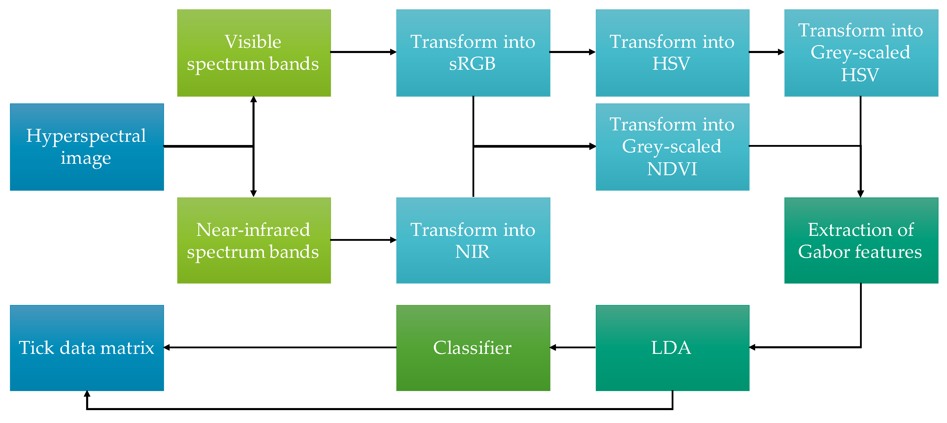
The proposed method, which is illustrated in Figure 2, firstly consists of the separation of the hyperspectral image’s bands to compute the standard Red, Green and Blue (sRGB) and Hue, Saturation and Value (HSV) colour spaces, as well as the Near-Infrared (NIR) channel and Normalised Difference Vegetation Index (NDVI) values. Secondly, the grey-scale representation of the HSV and NDVI images are utilised for feature extraction using a Gabor filter bank. Once the Gabor features are obtained, they are reduced through LDA and given to an ANN for classification. Finally, the classifier assigns a label to each one of the pixels, and they are saved in a tick data matrix with their reduced features, achieving the organisation stage of the data processing pipeline.

The transformations, Gabor features extraction, reduction process and architecture of the classifier are detailed in the following subsections. Furthermore, the test images and the experiments to validate the method are described.

2.1. Separation of Visible and Near-Infrared Spectrum Bands

The data structure commonly used to represent a hyperspectral image consists of a data cube composed of various matrices, where each element of a matrix records a band of the electromagnetic spectrum. These images have a high spectral resolution describing even more than a hundred bands, and each pixel represents a spectral signal. Therefore, the whole image can be denoted as in Equation (1):

$$X=\left\{x_i\in {\mathbb{R}}^B,i=1,2,\dots ,P\right\},$$

(1)

being X an image with P number of pixels, and each pixel x contains B number of bands.

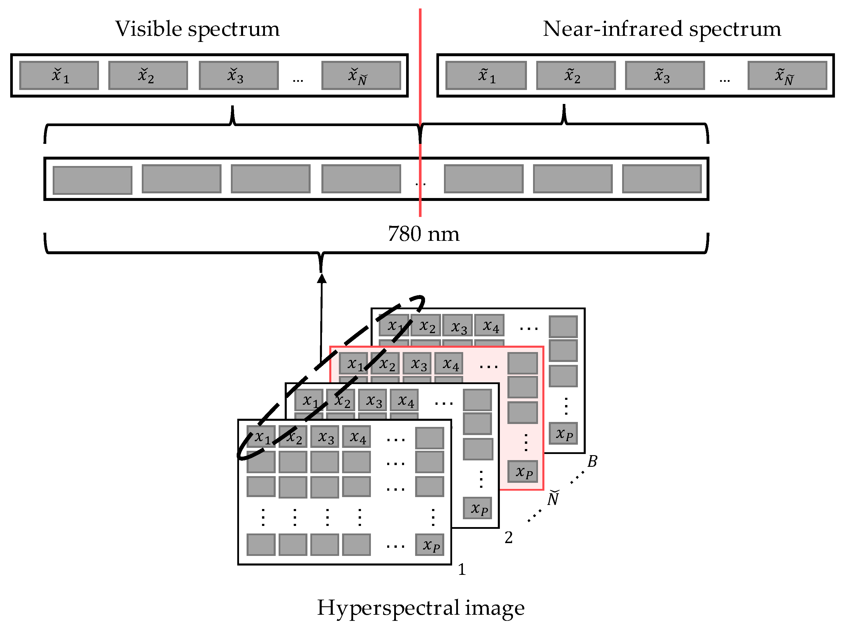
The spectrum of the pixel can be divided into visible and near-infrared sections as illustrated in Figure 3, where ${\check{x}}_i$, ∀$i=1,\dots ,\check{N}$, are the available values of the bands measured on the visible spectrum, which can be from 380 to 780 nanometres; and ${\tilde{x}}_i$, ∀$i=1,\dots ,\tilde{N}$, correspond to the available values of the near-infrared bands that can be measured up to 1200 nanometres.

2.2. Colour Space Transformation Methods

Once the visible and near-infrared bands are separated, each section can be transformed into different colour spaces or indices. This subsection describes the process to compute CIE XYZ, sRGB, HSV, NIR channel and NDVI values.

The bands in the visible spectrum have to be transformed into tri-stimulus to be compatible with other spaces. The transformation is achieved employing the matching functions W, $\mathcal{X}$, $\mathcal{Y}$ and $\mathcal{Z}$, which are defined in a standard from the International Commission on Illumination (CIE) [30]. These functions and the normalisation constant $\mathcal{K}$ allow the mapping of the visible spectrum $\check{x}$ in the CIE XYZ colour space using the equations in [31].

The CIE XYZ space has a transformation function to the sRGB space using a linear transformation defined by CIE and the equations given in [32]. Furthermore, the sRGB values can be weighted using the Equation (2) to compute a grey-scale value $G_{RGB}$ in order to extract texture features in later stages:

$$\begin{array}{c}{G}_{RGB}=\left[\begin{array}{ccc}\hfill 76.2195& \hfill 149.6850& \hfill 29.0700\end{array}\right]\times \left[\begin{array}{c}{R}_{sRGB}\\ G_{sRGB}\\ B_{sRGB}\end{array}\right].\end{array}$$

(2)

The HSV colour space is robust to illumination changes since it separates and decorrelates the characteristics of the colours affected by brightness variations [33]. In this work, the HSV values have been computed from the sRGB channels normalised to the interval $\left[0,1\right]$ by means of [34]. Therefore, their grey-scale value $G_{HSV}$ is calculated with Equation (3):

$$\begin{array}{c}{G}_{HSV}=\left[\begin{array}{ccc}19435.9725\hfill & 38169.6750\hfill & 7412.8500\hfill \end{array}\right]\times \left[\begin{array}{c}{H}_{HSV}\\ S_{HSV}\\ V_{HSV}\end{array}\right].\end{array}$$

(3)

For the other segment of the pixel, the NIR channel is calculated with the energy of the near-infrared bands using Equation (4):

$$NIR=\sum _{i=1}^{\tilde{N}}{\tilde{x}}_i^2.$$

(4)

Nonetheless, the NIR representation needs to be in the interval $\left[0,255\right]$ to be compatible with the colour spaces described before. Consequently, its grey-scale value $G_{NIR}$ is obtained weighting the $NIR$ value by Equation (5):

$$G_{NIR}=\frac{255}{\tilde{m}}NIR,$$

(5)

where $\tilde{m}$ is the maximum value in the whole near-infrared image.

The components of colour spaces can be employed to compute different indices that reflect the conditions of the materials. One of these indices is the Normalised Difference Vegetation Index (NDVI), which distinguishes between the presence of healthy or gathered vegetation areas and scattered or unhealthy ones [35]. This index is widely used for different applications, for example, the distinction between urban and farmland areas [36], generation of damage assessment maps after natural disasters [37] and evaluation of vegetation cover and soil characterisation [38]. Moreover, it has achieved a greater overall accuracy rate classifying certain crops when it is merged with other characteristics such as texture features and the digital value of the pixel [39].

The NDVI representation requires the previously computed $G_{NIR}$ and $R_{sRGB}$ values to measure the vegetation’s reflection [40]. However, this index is in the range $\left[-1,1\right]$. Therefore, the NDVI is multiplied by 127.5 in agreement with the other grey-scale values utilised in the method as in Equation (6):

$$G_{NDVI}=127.5\left[\frac{G_{NIR}-R_{sRGB}}{G_{NIR}+R_{sRGB}}+1\right].$$

(6)

2.3. Gabor Features Extraction and Reduction with LDA

The data reduction can be performed by translating the original data into another space with a lower dimension. The transformation is usually applied using projection-based methods that can be categorised in supervised, such as LDA, and unsupervised, like PCA [41]. Both methods have been tested to decrement the number of spectral bands in multispectral images for land cover classification, where LDA has surpassed PCA in classification accuracy using an ANN [42]. Besides, the LDA approach can also be used for texture characteristics. For example, a variation inspired in LDA has been used to reduce the dimension of Gabor features extracted from gait images for human authentication purposes [43]. Consequently, LDA and Gabor features were employed for this work.

The grey-scaled images are filtered with a Gabor filter bank, resulting in a vector of features. Each feature corresponds to the pixel’s value in the image processed using a certain Gabor filter. The Gabor filter consists of a sinusoid with a Gaussian envelope, whose function in the frequency domain is given by Equation (7):

$$\begin{array}{c}H\left(u,v\right)=A{e}^{-0.5\frac{{\left(\dot{u}-F\right)}^2}{{\sigma }_u^2}+\frac{{\dot{v}}^2}{{\sigma }_v^2}};\\ \dot{u}=ucos\left(\theta \right)-vsin\left(\theta \right),\\ \dot{v}=usin\left(\theta \right)+vsin\left(\theta \right),\end{array}$$

(7)

where $A=2\pi {\sigma }_x{\sigma }_y$, being ${\sigma }_X$ and ${\sigma }_Y$ parameters of the Gaussian envelope. Moreover, ${\sigma }_u=\frac{1}{2\pi {\sigma }_x}$, ${\sigma }_v=\frac{1}{2\pi {\sigma }_y}$ and $F=\frac{1}{{\omega }_{\iota }}$, considering ${\omega }_{\iota }$ as the wavelength of the sinusoid.

The filter bank is constituted by variations in the parameters of Equation (7) to detect borders or textures in an image utilising different orientations and scales [44]. For this work, the wavelength configuration proposed by Jain and Farrokhnia [45] is employed as in Equation (8):

$$\begin{array}{c}{\omega }_{\iota }=\frac{4}{\sqrt{2}}{2}^{\iota },\iota =0,1,\dots ,\eta -1,\\ \eta =⌊{log}_2\left[\frac{\sqrt{2}}{4}\sqrt{{\left(\mathrm{height}\right)}^2+{\left(\mathrm{width}\right)}^2}\right]⌋-1,\end{array}$$

(8)

where the height and width of the image are considered, and $\eta$ is the number of wavelengths. Moreover, the orientations used for $\theta$ are $0^{\circ }$, ${45}^{\circ }$, ${90}^{\circ }$ and ${135}^{\circ }$, being $\Theta =4$. Consequently, the filter bank contains $\breve{N}$ filters:

$$\breve{N}=\Theta \eta .$$

(9)

Suppose two grey-scale representations of the image are employed. In that case, both are processed with the Gabor filter bank, and the ensued features’ vectors are merged in a single vector g one beside the other, giving the double of characteristics of a single representation ($2\breve{N}$, using Equation (9)). Since the Gabor features are numerous depending on the image’s size, a reduction with LDA is proposed.

The LDA method changes the coordinates of the input features to minimise the dispersion of the same class’ observations while the distance between samples of different classes is maximised [26]. This optimisation problem is solved satisfying the constraint in Equation (10):

$$\begin{array}{c}{\Phi }_{LDA}={arg\; max}_{\Phi }\left[\frac{|{\Phi }^T{M}_{between}\widehat{\Phi }|}{|{\Phi }^T{M}_{within}\Phi |}\right],\\ {\Phi }_{LDA}=\left[{\varphi }_1,{\varphi }_2,\dots {\varphi }_{K-1}\right],\end{array}$$

(10)

where $\varphi$ is an eigenvector corresponding to the eigenvalue $\lambda$ complying ${\lambda }_k>{\lambda }_{k+1}$, and K is the total number of classes.

LDA is a supervised method. Therefore, the matrices $M_{between}$ and $M_{within}$ use mean vectors ${\mu }_k$ computed from the training observations g of each class k as in Equation (11):

$$\begin{array}{c}{M}_{between}={\ddot{P}}^{-1}\sum _{k=1}^K{\widehat{P}}_k\left({\mu }_k-\mu \right){\left({\mu }_k-\mu \right)}^T,\\ M_{within}={\ddot{P}}^{-1}\sum _{k=1}^K\sum _{p=1}^{{\widehat{P}}_k}\left(g_k^{\left(p\right)}-{\mu }_k\right){\left(g_k^{\left(p\right)}-{\mu }_k\right)}^T,\end{array}$$

(11)

where $\mu$ is the global mean of the training observations, and $\ddot{P}={\sum }_{k=1}^K{\widehat{P}}_k$, being ${\widehat{P}}_k$ the total number of training observations belonging to class k.

The data reduction is performed using the ${\Phi }_{LDA}$ matrix defined in Equation (10) as follows:

$$\mathcal{M}=\mathcal{S}\times {\Phi }_{LDA},\mathcal{S}\in {\mathbb{R}}^{\left(P\times \breve{N}\right)},{\Phi }_{LDA}\in {\mathbb{R}}^{\left(\breve{N}\times K-1\right)},$$

(12)

where $\mathcal{S}$ is a matrix with the extracted features of all the observations of the image stacked in rows, and $\mathcal{M}$ is also an observations’ matrix but with reduced features. Therefore, $2\breve{N}$ is employed instead of $\breve{N}$ in Equation (12) when two grey-scale representations are used for the features’ vector.

2.4. ANN Classifier Architecture

Once the data features have been obtained and reduced, a labelling process is needed to index the data. Therefore, a classifier such as SVM or ANN is implemented. In some cases, the SVM has obtained higher classification rates against ANN, especially in binary decisions such as the identification of corn presence [46]. On the other hand, another study has concluded that a Multilayer Perceptron (MLP) ANN can achieve an adequate classification accuracy surpassing the SVM for surface water mapping [47]. However, the ANN architectures can be computationally expensive depending on its structure [48].

The ANN architecture selected for the proposed method is the fully connected MLP. The employed structures have been denoted in this work as Neural Network Multilayer Perceptron followed by the number of neurons in their hidden layers (NNMLP-X_X). This architecture has the following definitions.

The MLP network has N layers with a certain quantity of neurons. Then, the set of the neurons that composes the network can be denoted as:

$$C=\left\{c_d\in \mathbb{Z},d=1,\dots ,N\right\},$$

(13)

being $c_d$ the number of units in layer d. A bias unit is implemented in each hidden layer. Nevertheless, it has not been included in Equation (13).

Since it is a fully-connected network, the weights associated to the neurons can be described as a matrix $\gamma$ for each layer, building the following set:

$$\Gamma =\left\{{\gamma }^{\left(i\right)}\in {\mathbb{R}}^{\left(c_d+1\right)\times c_{d+1}},i=1,\dots ,N-1\right\}.$$

(14)

Each layer requires an input matrix to perform the weighting and activation operations, which in the hidden layers corresponds to the output matrix of the previous layer. The input matrices for each layer are denoted as $\varrho$ an their set is given in the subsequent equation:

$$\Pi =\left\{{\varrho }^{\left(i\right)}\in {\mathbb{R}}^{P\times \left(c_d+1\right)},i=1,\dots ,N\right\}.$$

(15)

Inside each layer, the weighting is performed using Equations (14) and (15) as follows:

$${\varpi }^{\left(i\right)}={\varrho }^{\left(i\right)}\times {\gamma }^{\left(i\right)}.$$

(16)

The weighted values in ${\varpi }^{\left(i\right)}$ are utilised in the sigmoid activation function given in Equation (17) [49]:

$${\Delta }_{\left(i\right)}={\left[1+e^{{\varpi }^{\left(i\right)}}\right]}^{-1},$$

(17)

where ${\Delta }_{\left(i\right)}$ is used as the input matrix for the layer $i+1$. The output layer, which is class ordered, only performs a maximum operation to activate the neuron with the highest value. Afterwards, the result is translated to a digit that represents the class. This label is merged with the $\mathcal{M}$ matrix to conform the tick data matrix.

The back-propagation algorithm was employed for training the networks. The cost function used in this work is denoted in Equation (18):

$$\begin{array}{c}E\left(\gamma \right)=-{\ddot{P}}^{-1}\sum _{p=1}^{\ddot{P}}\sum _{k=1}^K\left[{\alpha }_k^{\left(p\right)}log\left(\Delta \right)+\left(1-{\alpha }_k^{\left(p\right)}\right)log\left(1-\Delta \right)\right]+\epsilon ,\\ \epsilon =0.25{\ddot{P}}^{-1}\left[\sum _{i=1}^{N-1}\sum _{r=1}^{c_{i+1}}\sum _{j=1}^{c_i}{\left({\gamma }_{r,j}^{\left(i\right)}\right)}^2\right],\end{array}$$

(18)

when ${\alpha }_k$ is a training binary vector activated in their corresponding class position, and $\ddot{P}$ is the total number of training observations.

The selected structures to perform the labelling are constituted by an input layer with the number of features as the number of neurons, two hidden layers and an output layer with a quantity equal to the number of classes. These structures are NNMLP-11_22 and NNMLP-F_2F. The first hidden layer of NNMLP-11_22 contains 11 neurons, and its second has 22, while NNMLP-F_2F has the number of input features in the first hidden layer and double of the features’ quantity in the second one.

2.5. Experimental Setup

The proposed method utilises the grey-scale representation of the image in HSV from Equation (3) and NDVI from Equation (6) to extract the Gabor features. Therefore, the grey-scale representations were changed for comparison with the following denotations: RGB for $G_{RGB}$ from Equation (2), NIR for $G_{NIR}$ from Equation (5) and NDVI for using only the grey-scaled NDVI image. Moreover, the combinations of RGB-NIR, RGB-NDVI and HSV-NIR features are also tested. The proposed method is identified as HSV-NDVI with NNMLP-11_22.

In order to verify the performance of the classifier, NNMLP-11_22 and NNMLP-F_2F are compared with the SVM. Then, the method using LDA as the reduction method and SVM as the classifier is denoted as LDA-SVM.

Since the proposed method reduces the features’ dimension, a variant without reduction classified with the SVM was also tested and compared. This variant is labelled as SVM in the results.

The experiments were executed using a processor Quad-Core Intel Core i7 2.7 GHz and 16 GB 2133 MHz RAM.

2.5.1. Test Images

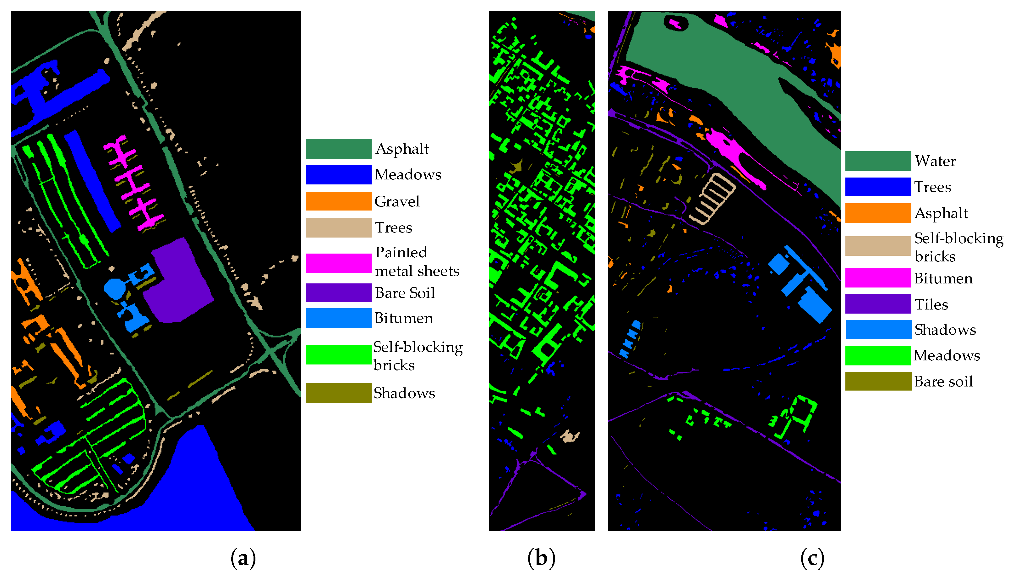
The hyperspectral images employed for testing correspond to the urban landscapes of the data sets collected by the Computer Intelligence Group (GIC) from the Basque University (UPV/EHU) available in [50]. A point worth mentioning is that the images have been employed as they are presented in this repository. However, the Pavia Center image was divided into Pavia Left and Pavia Right to test different classes and image sizes. The images’ properties are given in

Table 1. Properties of the test hyperspectral images.

Image	Bands	Size	Labelled Pixels	Classes
Pavia University	103	610 × 340	42,776	9
Pavia Right	102	1096 × 492	103,539	9
Pavia Left	102	1096 × 223	44,613	8

, and their reference maps for classification are displayed in Figure 4.

2.5.2. Training Setup

The classifiers and LDA were trained using three schemes for comparison. A different percentage of observations were randomly selected from each data set in each scenario: $30\%$, $40\%$ and $50\%$. Later, the observations are employed to compute the LDA matrix and to train the classifiers. This process is performed ten times to calculate average results.

2.5.3. Quality Measures

The measures used to evaluate the performance of the algorithms are the Overall Accuracy (OA) and the $\kappa$ coefficient given in [47]. In addition, the strength of agreement of the $\kappa$ coefficient is evaluated using the categories stated in [51].

The data processing pipeline requires a balance in accuracy, run-time and resources usage. Therefore, another measure employed is the Reduction Efficiency Coefficient (REC) [52]. This coefficient measures the reduction performance according to classification OA and the number of features reduced, achieving values near 1 when there is a good classification combined with a high reduction of features:

$$REC=OA\left(1-\frac{\widehat{\mathcal{F}}}{\mathcal{F}}\right),$$

(19)

where $\widehat{\mathcal{F}}$ is the number of features employed after the reduction, and $\mathcal{F}$ is the original number of features. Since the objective of the proposed method is the reduction and organisation of the hyperspectral information, $\mathcal{F}$ is set as the original number of bands, and the number of features given to the classifier is used as $\widehat{\mathcal{F}}$.

3. Results

The results obtained from the experiments described above are reported in this section. Firstly, a visual comparison between the colour spaces and indices employed is presented. Then, the results related to the overall accuracy of the classification, such as standard deviation, $\kappa$ coefficient and REC, are given. Finally, the training and evaluation time is displayed.

3.1. Colour and Indices Comparison

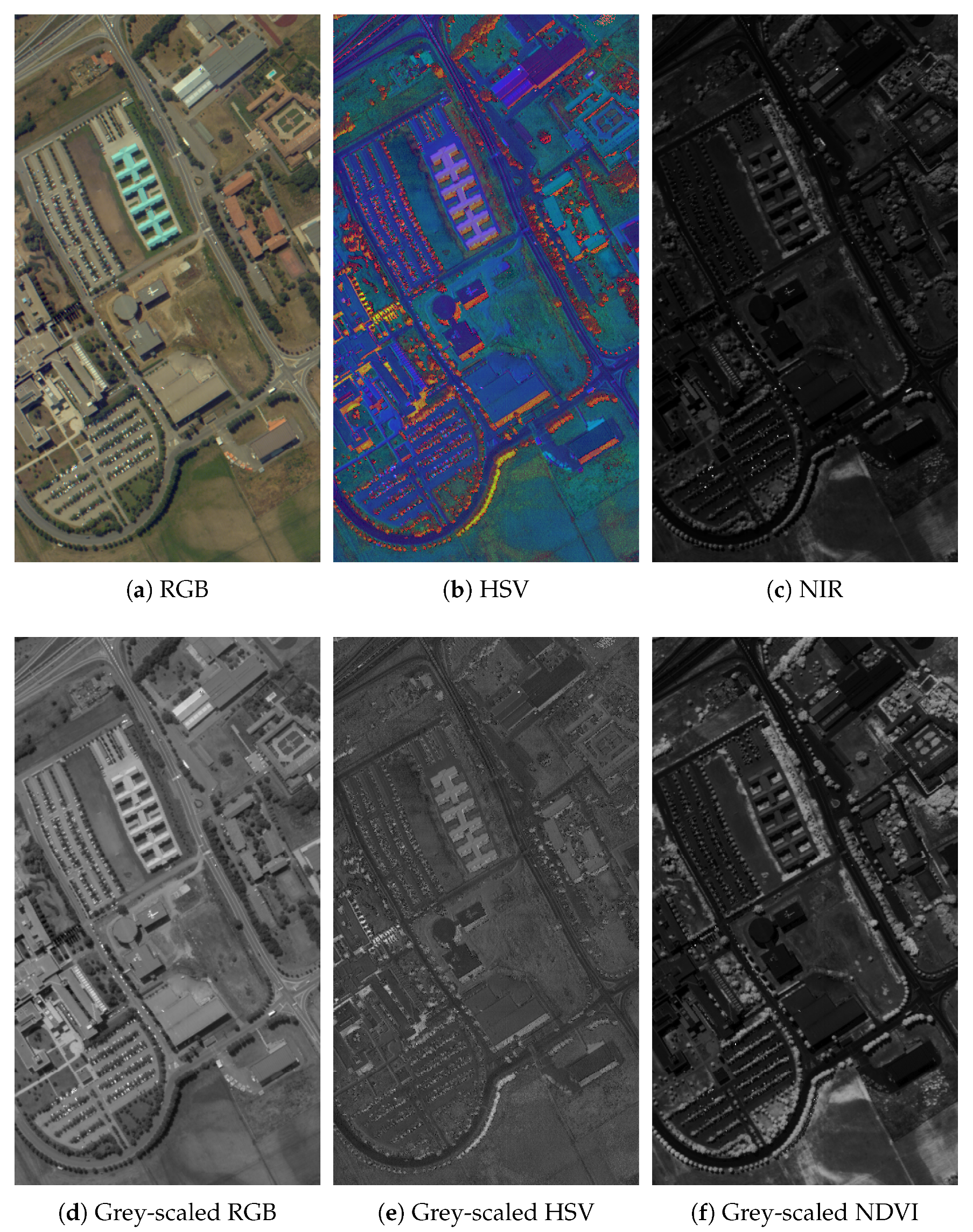
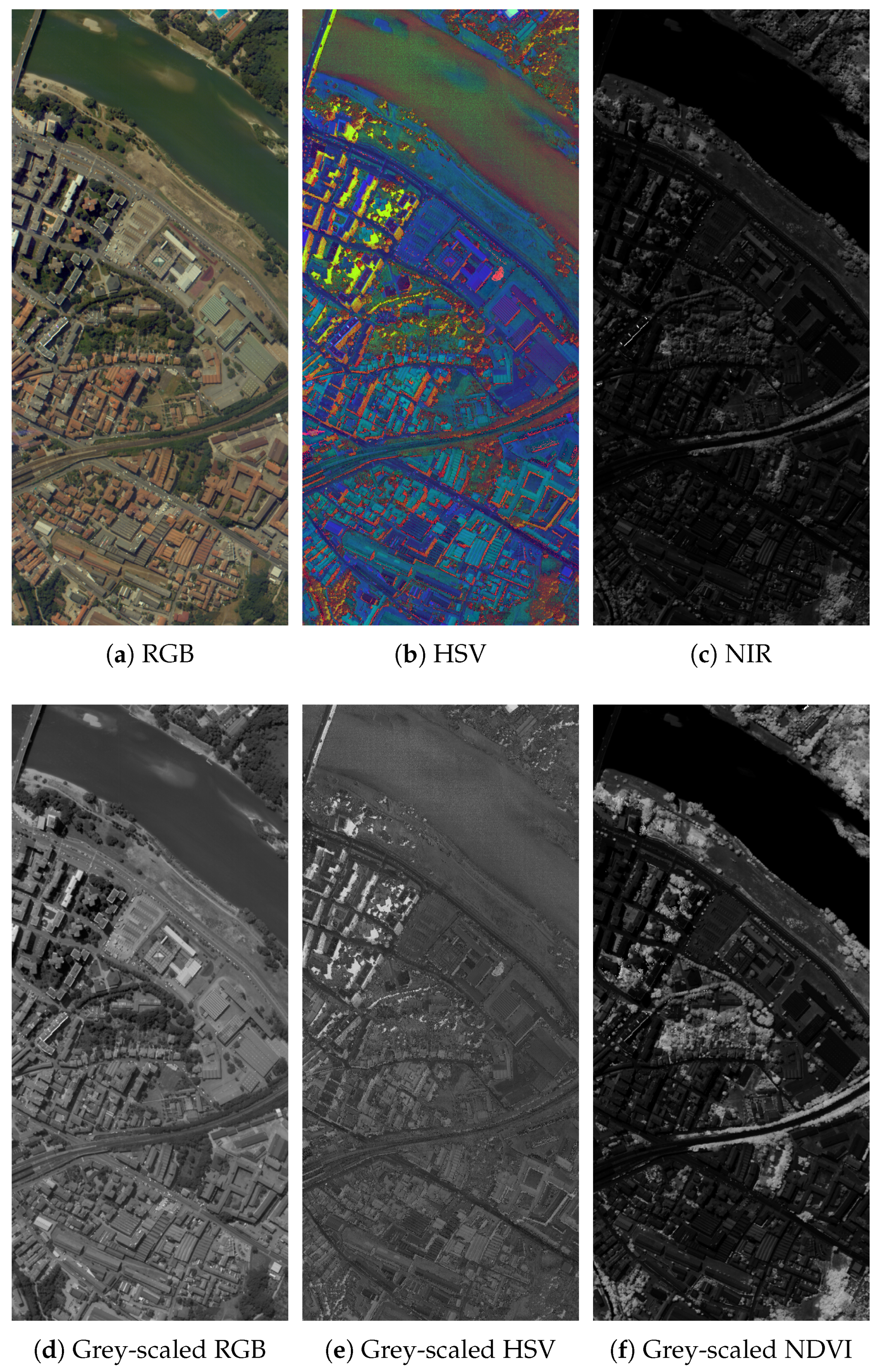
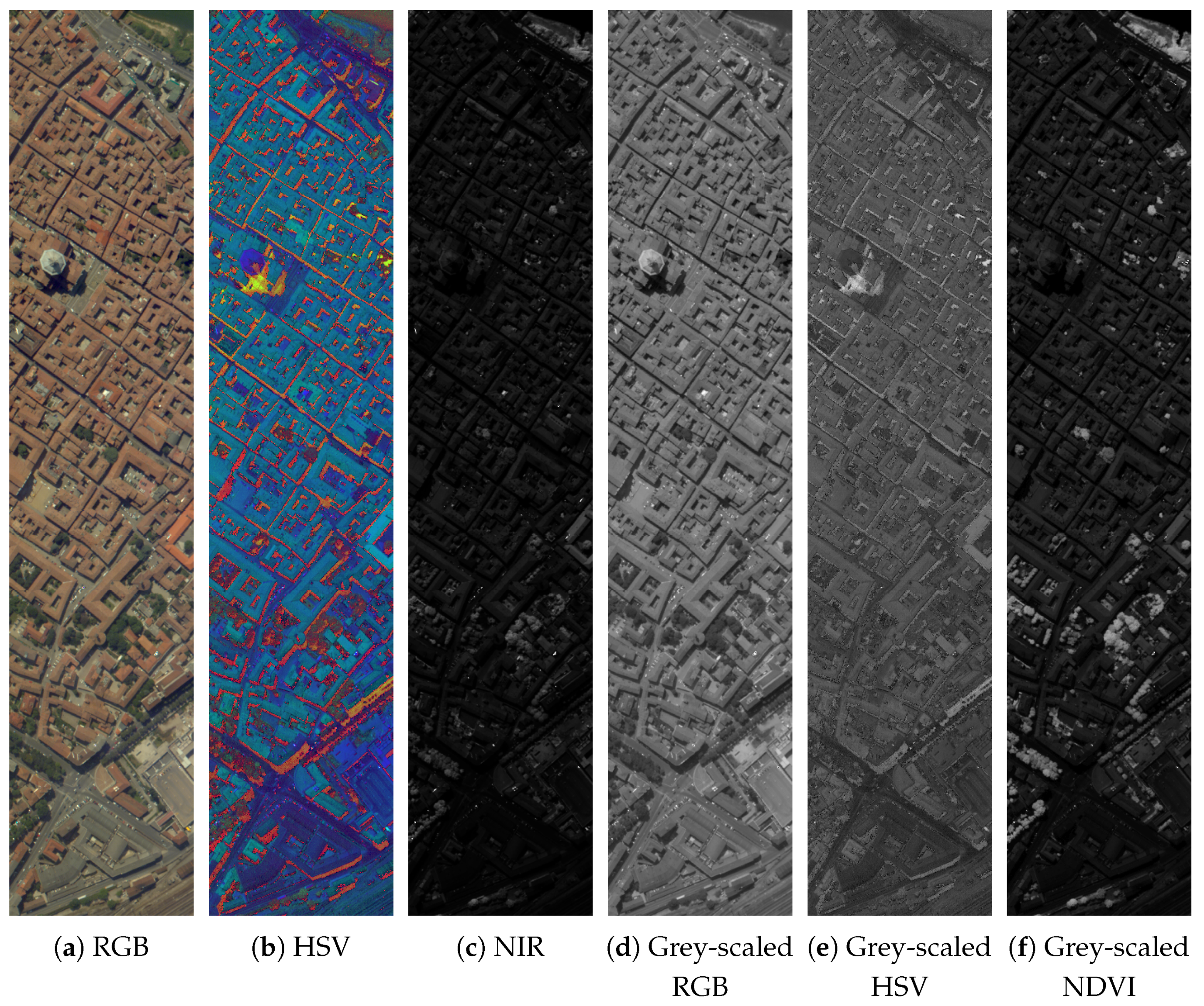
The classification accuracy comparison is related to the change of the selected grey-scale images for Gabor features extractions. Then, the grey-scale representations of the testing images and their colour images have been contrasted in Figure 5, Figure 6 and Figure 7.

It can be observed that in HSV images in Figure 5b, Figure 6b and Figure 7b, the pixels representing an object in the images are coloured with similar tones, and the difference between the adjacent objects is highlighted. Therefore, their textures suffer changes when they are transformed to the grey-scaled representation, such as in Figure 5e, Figure 6e and Figure 7e. Besides, the NIR representations in Figure 5c, Figure 6c and Figure 7c present richer textures for vegetation than the grey-scaled RGB ones (Figure 5d, Figure 6d and Figure 7d. Nonetheless, Figure 5f, Figure 6f and Figure 7f highly feature live vegetation areas since the NDVI index possesses this property.

3.2. Variation in the Number of Training Samples

The LDA method, as well as the selected classifiers, are supervised algorithms. Therefore, they need a certain amount of information to be trained. However, they usually have to work with a limited amount of available labelled data, experiencing unexpected behaviours when the volume of the training set is changed.

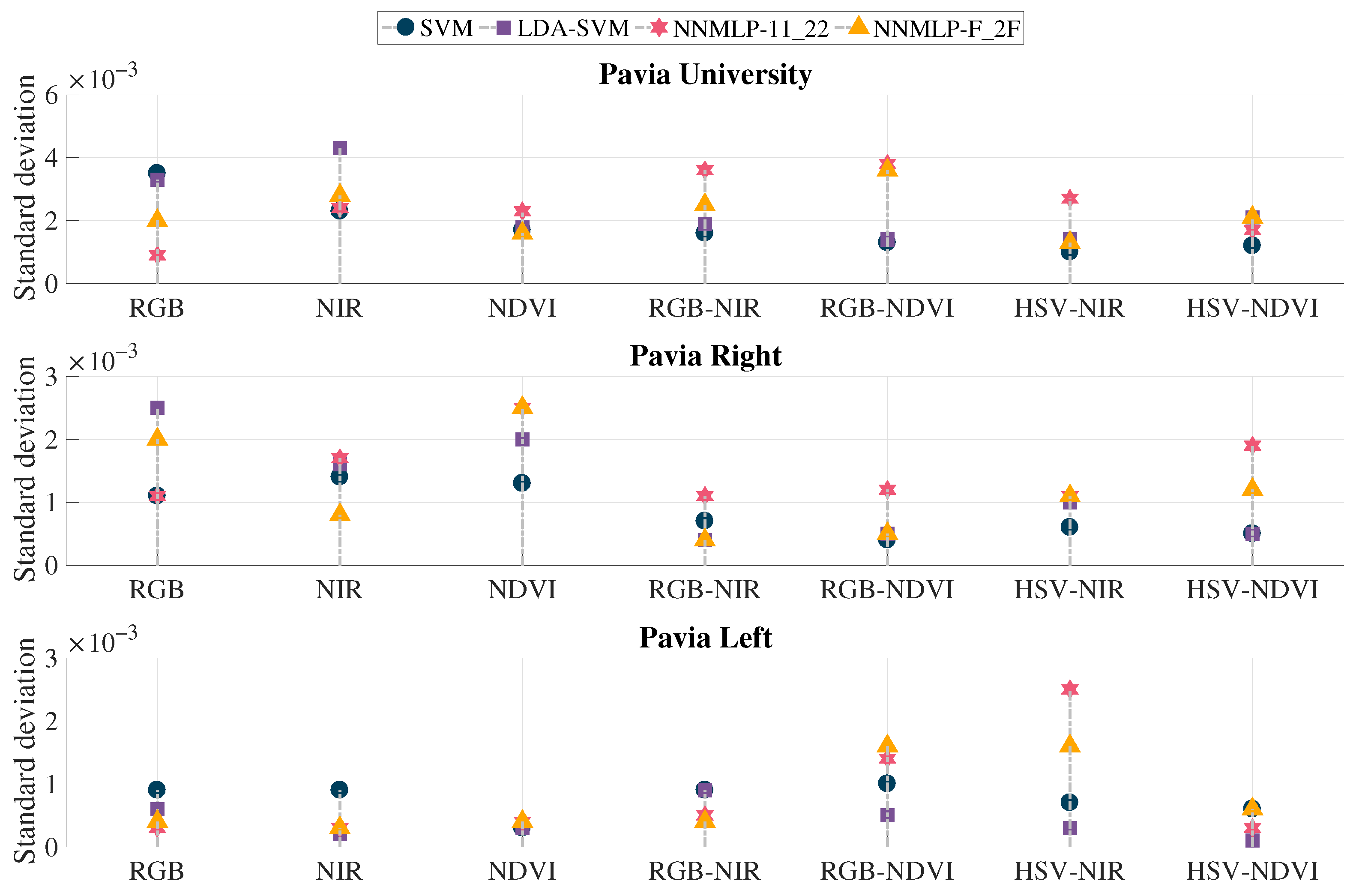
The proposed method’s performance is validated by computing the overall accuracy values resulted from the testing sets given by the three training scenarios. The overall accuracy’s standard deviation indicates a behaviour pattern. If the classification accuracy significantly changes when the number of training features is modified, the standard deviation increases. On the contrary, if the accuracy remains stable, the standard deviation is low. These results are displayed in Figure 8.

All the evaluated methods presented a standard deviation lower than 0.005, being the range of accuracy in the interval from zero up to one. The last means that the results fluctuate lower than 0.5% with the change in training observations. The highest deviation is presented in Pavia University’s image using the method NIR with LDA-SVM reaching a value of 0.0043, followed by RGB-NDVI with both ANN classifiers: NNMLP-11_22 ensuing 0.0038, and NNMLP-F_2F resulting in 0.0036. The lowest value is presented in the image Pavia Left using HSV-NDVI with LDA-SVM, being 0.0001. Finally, the proposed method (HSV-NDVI with NNMLP-11_22) achieved standard deviations lower than 0.002 for the test images, implying a fluctuation of around 0.2% in the classification accuracy rates.

3.3. Classification Overall Accuracy and $\kappa$ Coefficient

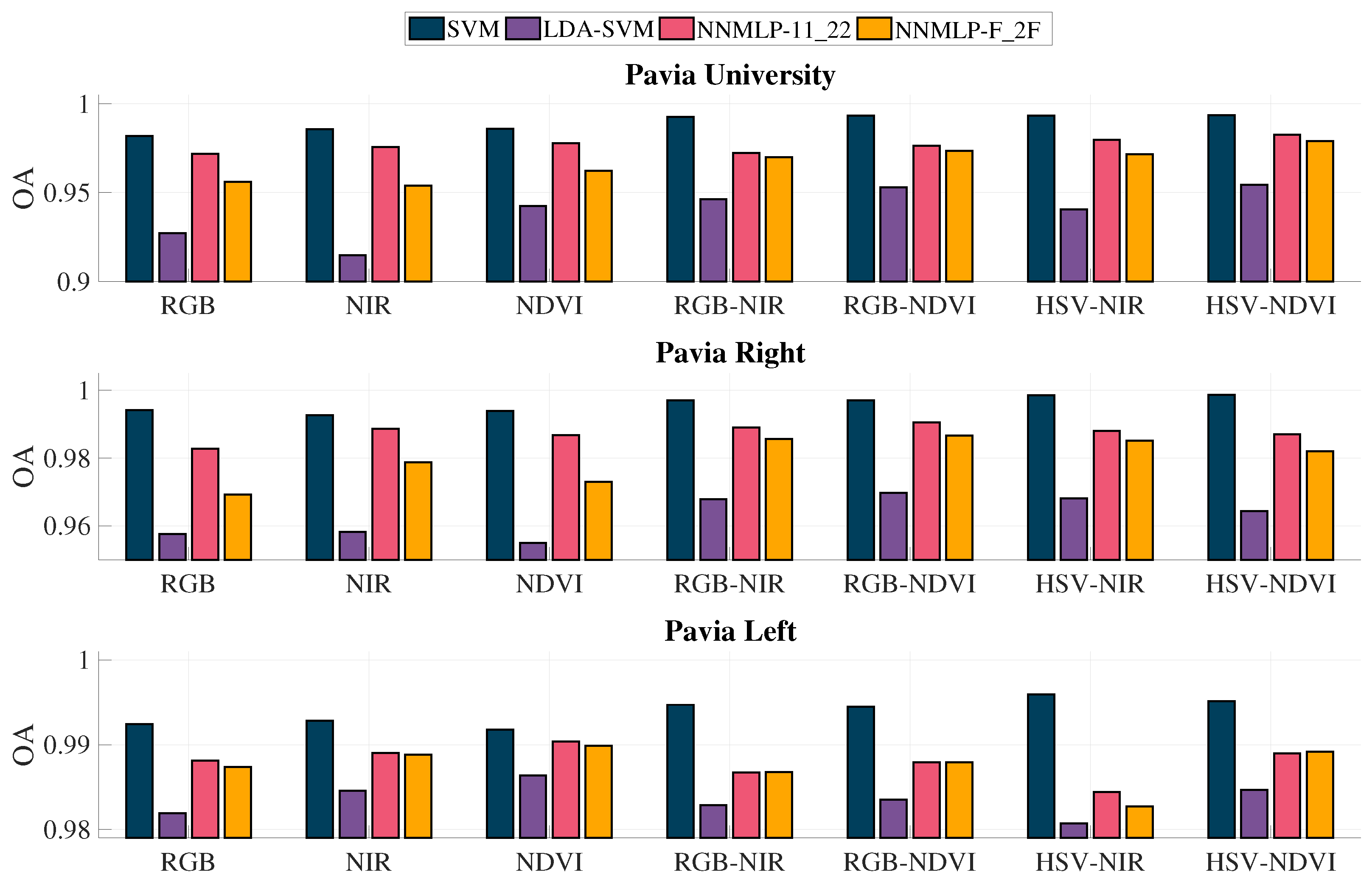
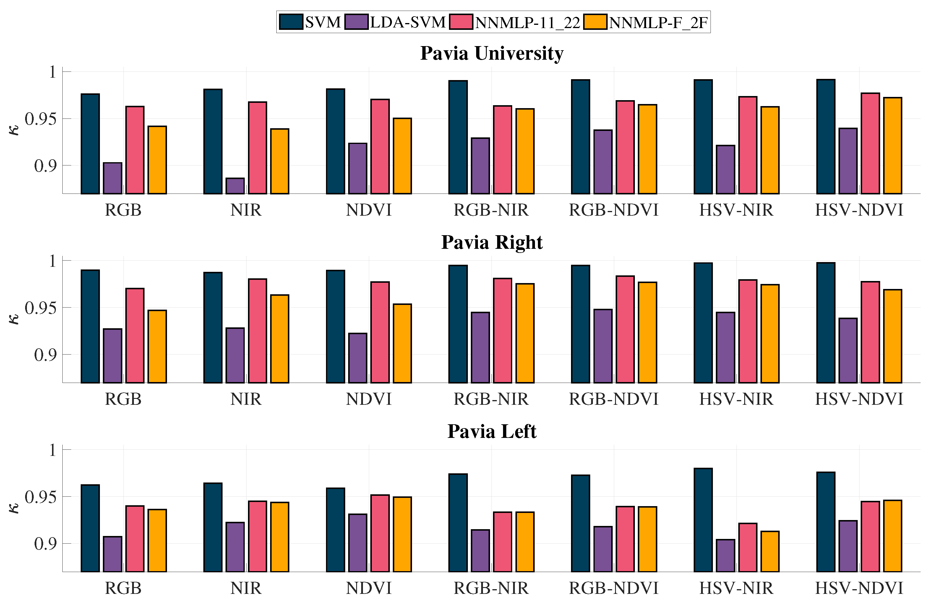
The classification accuracy’s standard deviation does not exceed 0.005; hence the testing sets of the 40% training scenario were selected for the comparison of the overall accuracy and $\kappa$ coefficient. Figure 9 contains the overall accuracy results for the methods used in the evaluation, while Figure 10 shows the resulted $\kappa$ coefficients.

It can be observed that the methods employing two grey-scaled representations for feature extraction achieved better OA using the methodology without LDA (denoted as SVM). Furthermore, the process without LDA has the best accuracy rates for all the grey-scale representations’ combinations, being the highest HSV-NIR and HSV-NDVI. Besides, the NNMLP-11_22 classifier resulted in better OA than NNMLP-F_2F and LDA-SVM, but consistently lower than SVM without LDA. Nonetheless, the average difference between SVM and NNMLP-11_22 is 0.0091, which represents a change of 0.9%.

The $\kappa$ coefficients are notably higher for SVM followed by NNMLP-11_22 for all the grey-scale representations’ combinations, while LDA-SVM’s results are the worst among all. The lowest value is 0.8863, which is derived from NIR with LDA-SVM. Nevertheless, the $\kappa$ coefficients can be grouped in categories according to the strength of agreement between the OA and the expected accuracy ensued by chance [52]. The $\kappa$ values should fall in the categories $\left[0.61,0.80\right]$ and $\left[0.81,1.00\right]$, which correspond to Substantial and Almost perfect, to evaluate a classification as adequate.

3.4. Reduction Efficiency

The reduction of the dimension should not significantly affect the classification accuracy for the organisation stage of the data processing pipeline. Therefore, REC is computed and shown in

Table 2. Overall accuracy and Reduction Efficiency Coefficient in percentage.

Pavia University
	SVM			NNMLP-11_22
Method	OA (%)	Features	REC (%)	OA (%)	Features	REC (%)
RGB	98.18	24	75.30	97.19	8	89.64
NIR	98.56	24	75.59	97.55	8	89.98
NDVI	98.58	24	75.61	97.77	8	90.17
RGB-NIR	99.26	48	53.01	97.23	8	89.68
RGB-NDVI	99.32	48	53.04	97.64	8	90.06
HSV-NIR	99.33	48	53.04	97.98	8	90.37
HSV-NDVI	99.34	48	53.05	98.26	8	90.63
Pavia Right
	SVM			NNMLP-11_22
Method	OA (%)	Features	REC (%)	OA (%)	Features	REC (%)
RGB	99.40	28	72.12	98.27	8	90.57
NIR	99.26	28	72.01	98.86	8	91.11
NDVI	99.38	28	72.10	98.68	8	90.94
RGB-NIR	99.69	56	44.96	98.89	8	91.14
RGB-NDVI	99.69	56	44.96	99.04	8	91.27
HSV-NIR	99.85	56	45.03	98.80	8	91.05
HSV-NDVI	99.86	56	45.04	98.70	8	90.95
Pavia Left
	SVM			NNMLP-11_22
Method	OA (%)	Features	REC (%)	OA (%)	Features	REC (%)
RGB	99.24	28	72.00	98.81	7	92.03
NIR	99.28	28	72.03	98.90	7	92.12
NDVI	99.18	28	71.95	99.04	7	92.24
RGB-NIR	99.47	56	44.86	98.67	7	91.90
RGB-NDVI	99.45	56	44.85	98.79	7	92.01
HSV-NIR	99.59	56	44.91	98.44	7	91.68
HSV-NDVI	99.51	56	44.88	98.90	7	92.11

, where only SVM and NNMLP-11_22 are contrasted because they were the methods that achieved better OA results.

The method without LDA reduction had lower results for all the grey-scale representations due to the number of features employed for classification. In contrast, NNMLP-11_22, which utilises LDA before the classification, achieved better REC. Then, using this method, the best REC for Pavia University was produced by HSV-NDVI, HSV-NIR and NDVI. In Pavia Right, RGB-NDVI, RGB-NIR and NIR, left the proposed method in the fifth position. The best results for Pavia Left were NDVI, NIR and HSV-NDVI.

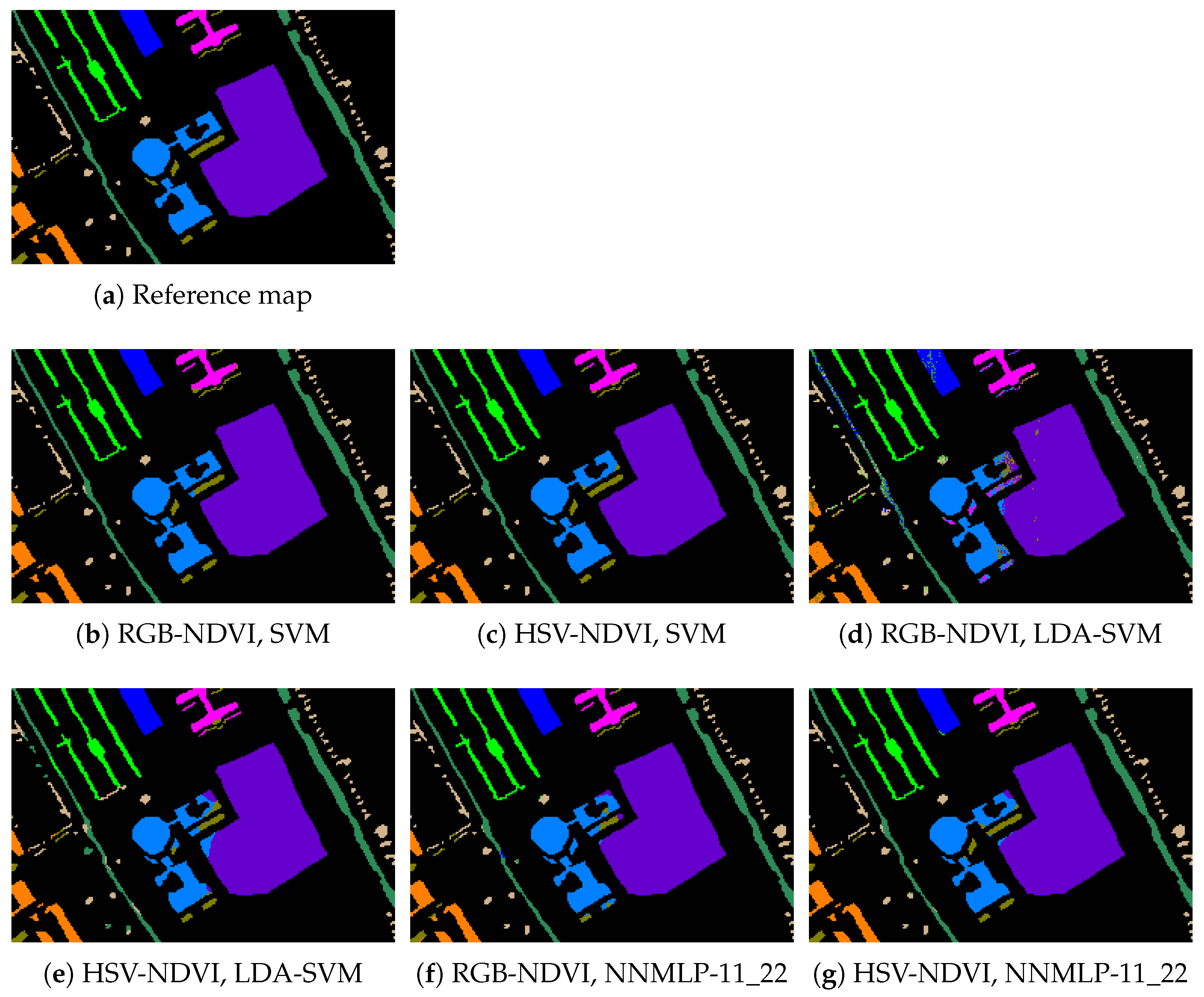
The image of Pavia University was the one with the lower REC for NNMLP-11_22. Therefore, the classification maps of the methods using RGB-NDVI and HSV-NDVI were contrasted in Figure 11. RGB-NDVI with LDA-SVM presented more inaccuracies in the labelling, although the mismatched pixels do not correspond to adjacent areas. The proposed method HSV-NDVI with NNMLP-11_22 correctly labelled the majority of the pixels that conform to an object of the same class: However, it has some inaccuracies for the pixels in the edge of adjacent objects. The HSV-NDVI using SVM without LDA reduced this kind of errors.

3.5. Training and Evaluation Time

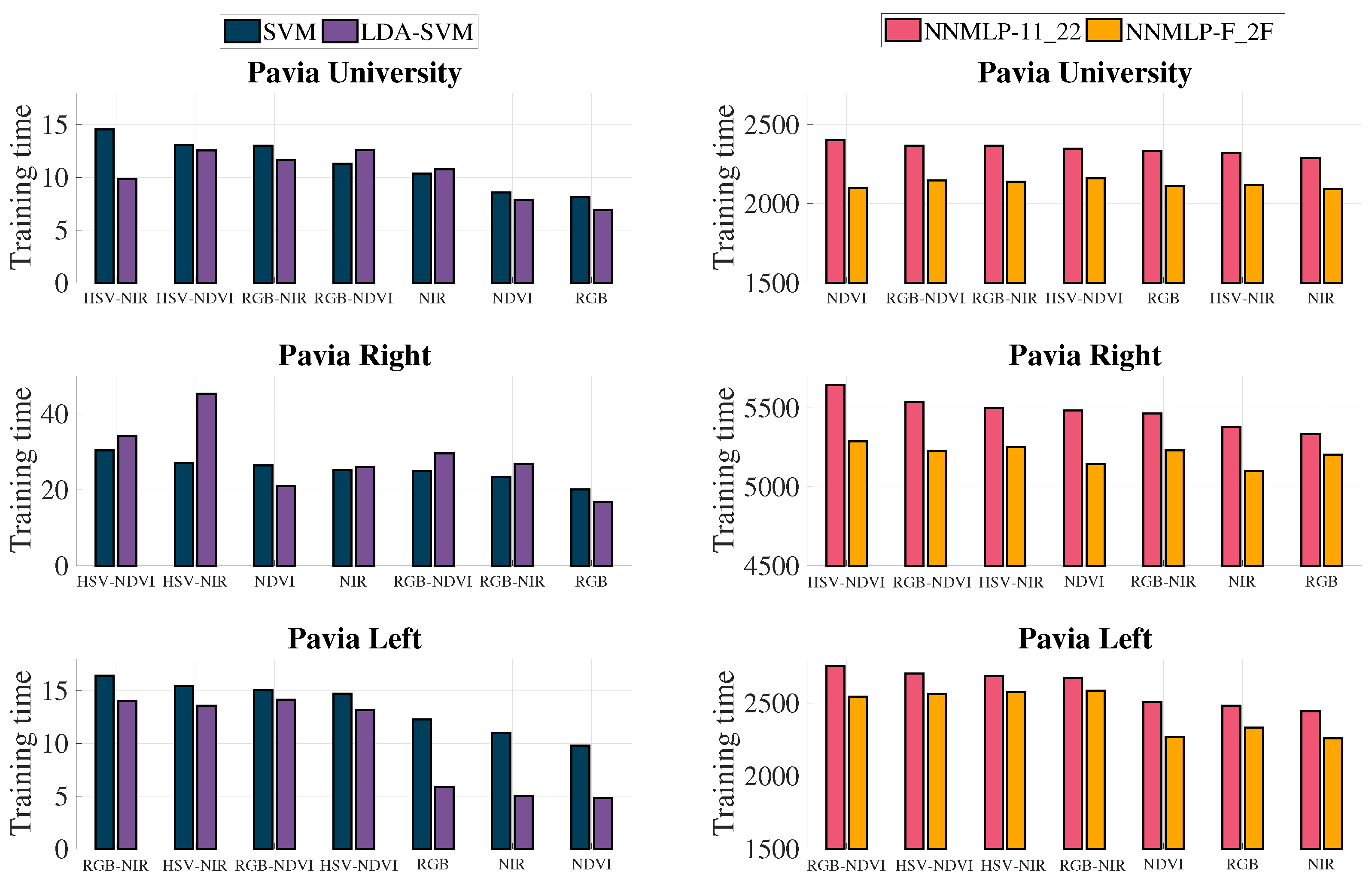
The training time of the algorithms was measured and plotted in Figure 12. It can be observed that the training of the approaches using SVM as the classifier is less expensive than those employing an ANN. However, it is noticed that the schemes with two grey-scale representations generally needed more time for training both classifiers.

The average evaluation time in seconds of SVM and NNMLP-11_22, which consists of the time needed to label all the observations once the classifier is trained, is displayed in

Table 3. Average evaluation time in seconds. NNMLP-11_22 is denoted as ANN.

	Pavia University		Pavia Right		Pavia Left
Method	SVM	ANN	SVM	ANN	SVM	ANN
RGB	4.3461	0.0189	14.6806	0.0384	1.7884	0.0224
NIR	4.3120	0.0229	16.1220	0.0465	1.4680	0.0188
NDVI	3.8108	0.0212	15.3272	0.0427	1.4689	0.0188
RGB_NIR	5.8720	0.0225	17.6227	0.0461	2.3725	0.0182
RGB_NDVI	5.3081	0.0207	16.4316	0.0419	2.2812	0.0185
HSV_NIR	5.8800	0.0194	16.6395	0.0433	2.2403	0.0161
HSV_NDVI	5.3234	0.0196	17.4909	0.0420	2.2420	0.0175

. The results show that the evaluation with SVM last at least $1\times {10}^2$ times the evaluation performed with NNMLP-11_22.

3.6. Application on a Multispectral Dataset

The proposed method has also been tested on multispectral images to evaluate the performance of the features’ classification. Three QuickBird images from Zurich Summer dataset [53] were employed, and their features were computed using the method HSV-NDVI. The images selected from the dataset present different class numbers and labels, which are related to urban scenes. The 5% of the labelled pixels was used for training, and the overall accuracy of the remaining pixels’ classification is given in

Table 4. Overall accuracy and features computed for multispectral images using HSV-NDVI method.

	SVM		LDA-SVM		NNMLP-11_22
Image	Features	OA (%)	Features	OA (%)	Features	OA (%)
Zh02	56	96.43	3	74.63	3	76.10
Zh03	56	97.75	6	88.77	6	95.25
Zh06	56	95.37	6	67.73	6	69.63

.

It can be observed that the Gabor filter feature extraction led to the computation of 56 features that were afterwards reduced up to $K-1$, being K the total number of classes. The overall accuracy descends when the SVM is employed with the reduced features. However, the NNMLP-11_22 classifier slightly increases the accuracy.

4. Discussion

This section analyses and explores the results reported in the previous section. The study aims to propose a method that transforms the acquired data into features that could be organised to reduce the burden of machine learning algorithms in further stages of the data processing pipeline for urban scenes.

Then, experiments using reduced and non-reduced features were conducted to test the hypothesis in Reddy et al. [29] that dimensionality reduction techniques do not significantly impact the performance of machine learning algorithms. Reddy et al. compared PCA against LDA for the features’ reduction registering competitive results using the SVM classifier. Therefore, the study of Seng and Ang [28] was taken into consideration to select the LDA method to reduce the extracted features because their experiments showed a great advantage of using LDA over PCA in face recognition datasets. However, both works agree on the need of testing the reduction on other features and classifiers.

Consequently, this work contrasts the base features for reduction using NDVI due to the analysis of features’ importance for crop information extraction given in Li et al. [46]. Furthermore, the HSV colour space is also compared because its performance surpassed RGB in crop classification as showed in Sandoval et al. [54]. Then, these indices were evaluated for urban classes.

The first comparison is performed using the standard deviation of the overall accuracy to evaluate the effects of the variation in the number of samples on the classification rates. The results suggest that the compared methods minimally change their behaviour in these conditions because all the evaluated methods had a standard deviation lower than $5\times {10}^{-3}$; specifically, the method HSV-NDVI classified with NNMLP-11_22, whose fluctuation is around 0.2%. Therefore, the compared methods permit to be implemented in applications with different training sets’ sizes without markedly changes in their results. Nonetheless, the features obtained from the grey-scaled RGB image generally had a higher deviation despite the classifier, especially in Pavia University’s image using SVM. This may be due to the characteristics of the RGB colour space.

The RGB space has a strong correlation between its channels, making its grey-scale representation less informative than the others presented in this study because it does not spotlight particular objects. Therefore, the training stage can be affected depending on the amount of information provided to find the decision rules. Then, the different grey-scale representations could be used for other applications where their attributes could highlight objects of interest. In this case, the grey-scaled HSV representation allowed the differentiation between adjacent objects, and the NDVI highlighted the vegetation areas. Besides, HSV-NDVI performed a better classification while the features were not reduced. Therefore, their reduced attributes may contain more discriminative information directly depending on the application.

In terms of classification rates, the SVM approach without LDA reduction led to the highest results, followed by the proposed method and the others based on it but with a combination of grey-scaled representations. The third position corresponds to the reduced features using the NNMLP-F_2F classifier. Finally, the LDA-SVM method ensued the worst results. Thus, the SVM classifier was affected by the data transformation using LDA. Although LDA-SVM’s OA is above 0.9, it is significantly disadvantaged against the SVM with non-reduced features having a difference of up to 6%. Consequently, the hypothesis of non-significant impact due to reduction presented by Reddy et al. [29] cannot apply for the compared features since their work showed a difference in the overall accuracy of 0.79% for their primary dataset’s classification. However, the suggestion of using a more robust classifier, which is presented in the study of Seng and Ang [28], is feasible.

An ANN can be employed for the classification of texture features. For example, Li et al. [46] compared SVM against a back-propagated ANN for the classification of texture and spectral characteristics. Their results are variant in the three datasets utilised. For binary classification, the SVM obtained better OA than ANN in their experiments. The lowest difference between the OA of SVM and ANN was 0.11%, while the highest consisted of 6.35%. Moreover, the difference in the $\kappa$ coefficient was up to 32.05%. Nevertheless, NNMLP-11_22 and NNMLP-F_2F maintained $\kappa$ values above 0.9 in the three images employed, which means that these architectures are robust for the reduced Gabor features and can substitute the SVM, contrarily to the architecture of Li et al. [46]. Besides, NNMLP-11_22 achieved an overall accuracy increment compared to LDA-SVM. Therefore, the average difference between the non-reduced features’ classification with SVM and the proposed method is lower than 1%.

The REC reported in the previous section shows that the SVM method without LDA reduces the initial number of bands, which are considered as the original features, up to 45%, and has the highest OA values. However, its REC is steadily diminished compared with the proposed method because it performed a reduction up to 87.5% of the original features. Therefore, the technique with non-reduced features can achieve higher classification rates. Nonetheless, the reduction with LDA and classification with NNMLP-11_22 achieved similar overall accuracy values with fewer features, which also benefits the evaluation time. The NNMLP-11_22 took less than 1.3% of the time spent by SVM for valuation.

The ANNMLP-F_2F is an architecture adjusted to the number of input features, and it has led to reasonable classification rates for pixel-wise attributes. Nevertheless, its classification performance was overcome by NNMLP-11_22, which has demonstrated its robustness with other texture features and reduction approaches [55]. However, the flexible structure of NNMLP-F_2F allows a lower training time for reduced attributes compared to NNMLP-11_22 because the number of characteristics employed in this study does not exceed eight units.

The training stage of the NNMLP-11_22 is significantly more expensive than the compared methods, especially against the SVM approach. However, the evaluation time is dramatically lower. The training stage of the classifiers is usually performed offline. Consequently, the training time does not affect the organisation stage as long as the classifier configuration has been already established. Contrarily, the evaluation time is crucial to maintain the continuous flow of input data.

The proposed scheme presents some disadvantages. The number of classes needs to be fixed according to the elements planned for the indexation. Therefore, the data requires a new transformation process if there are changes in the semantics of the indices. In addition, further analysis is needed with a more extensive dataset with labelled pixels. Moreover, the test using multispectral images indicates that the proposed method could be applied for their labelling and consequently a thematic organisation. The proposed classifier increased the overall accuracy in comparison with the SVM. Furthermore, a classification near 70% was achieved in the worst case. However, the accuracy had a considerable difference between the reduced and non-reduced characteristics in most of the cases. Thus, the features for this case need to be refined to achieve a higher classification accuracy.

5. Conclusions

A method for the organisation stage of a data processing pipeline was proposed. This method employs the grey-scaled HSV representation and the grey-scaled NDVI of a hyperspectral image to extract texture features using a Gabor filter bank. Then, the features are reduced through LDA and classified utilising an ANN architecture to compose a tick data matrix with indices that can be retrieved for further analysis in the hyperspectral images’ processing pipeline for urban remote sensing applications. The proposed method was tested using different grey-scaled representations and compared with non-reduced features using the SVM as the classifier. This approach achieved lower classification accuracy than the method using SVM. However, it can balance the reduction of features and classification rates according to the simulation results, which is desirable for performing the organisation stage. Furthermore, the ANN has demonstrated a lower evaluation time than SVM, allowing the processing of a large amount of data in a short time. Nevertheless, the proposed method should be refined to perform real-time processing to be fully implemented in an urban remote sensing application.