Article

Bearings-Only Target Tracking with an Unbiased Pseudo-Linear Kalman Filter

1
Institute of Acoustics, Chinese Academy of Sciences, Beijing 100190, China
2
School of Electronic, Electrical and Communication, University of Chinese Academy of Sciences, Beijing 100864, China
3
Department of Engineering, University of Niccolo Cusano, via Don Carlo Gnocchi 3, 00166 Rome, Italy
*
Author to whom correspondence should be addressed.
Remote Sens. 2021, 13(15), 2915; https://doi.org/10.3390/rs13152915
Submission received: 18 May 2021 / Revised: 9 July 2021 / Accepted: 10 July 2021 / Published: 24 July 2021
(This article belongs to the Special Issue Radar Signal Processing for Target Tracking)

Abstract

:
In bearings-only target tracking, the pseudo-linear Kalman filter (PLKF) attracts much attention because of its stability and its low computational burden. However, the PLKF’s measurement vector and the pseudo-linear noise are correlated, which makes it suffer from bias problems. Although the bias-compensated PLKF (BC–PLKF) and the instrumental variable-based PLKF (IV–PLKF) can eliminate the bias, they only work well when the target behaves with non-manoeuvring movement. To extend the PLKF to the manoeuvring target tracking scenario, an unbiased PLKF (UB–PLKF) algorithm, which splits the noise away from the measurement vector directly, is proposed. Based on the results of the UB–PLKF, we also propose its velocity-constrained version (VC–PLKF) to further improve the performance. Simulations show that the UB–PLKF and VC–PLKF outperform the BC–PLKF and IV–PLKF both in non-manoeuvring and manoeuvring scenarios.

1. Introduction

Bearings-only tracking (BOT) comprises estimating a target’s state from bearing measurements received by an observer [1]. It plays an important role in both military and civil applications, for example, underwater surveillance [2,3], 3-D passive target tracking [4,5,6,7] and UAV (unmanned aerial vehicle) path planning [8,9,10,11]. However, the nonlinear relationship between the bearing measurements and the target state vector makes BOT a typical nonlinear filtering problem [12].
There are two common ways to deal with the nonlinearity in the BOT problem. The first way is to choose the nonlinear Bayesian filtering algorithms. Early approaches are based on the extended Kalman filter and its improved versions [1,13,14]. However, the extended Kalman filter uses the first-order Taylor expansion to replace the corresponding nonlinear function, which will certainly lead to truncation errors. Other more sophisticated Kalman filters, such as the unscented Kalman filter [15] and the cubature Kalman filter [16], applied to the BOT problem, can be found in [17,18]. Another important approach is based upon particle filtering (see, for instance, [19,20]). However, the high computational requirements of the particle filter would involve high-performance expensive hardware that discourages its implementation in BOT applications. It is important to also mention here the non-Bayesian-based shadowing filter that, recently, has been applied to the BOT problem [21]. However, such a filter is a kind of gradient descent algorithm, hence, it is highly sensitive to the step size as well as the computation of the Jacobian matrix [22].
Another way to cope with the nonlinearlity in BOT is to convert it into linear form, and the most common method used is the pseudo-linear Kalman filter (PLKF) [23]. It has lower computational complexity and is more robust compared with the nonlinear Bayesian filtering algorithms introduced above [24], and no other prior parameters are required compared with the shadowing filter. These advantages make the PLKF an attractive method for engineering. However, unlike the traditional Kalman filter, the PLKF measurement vector contains the bearing noise, which makes it correlated with the pseudo-linear noise. This correlation leads to bias problems for the PLKF. To improve the PLKF performance, the instantaneous bias of PLKF is analysed in [25], and two improved PLKF algorithms, the bias-compensated PLKF (BC–PLKF) and the instrumental variable-based PLKF (IV–PLKF), are proposed. The BC–PLKF subtracts the approximated bias from the estimate of the PLKF to reduce the bias. The IV–PLKF utilizes the results of the BC–PLKF to construct a noise-free measurement vector, and its asymptotic unbiasedness has been proved in [25,26]. Although BC–PLKF and IV–PLKF effectiveness has been verified in [25] when the target moves without manoeuvring, their performance in the manoeuvring target tracking scenario may be unsatisfactory. It is not surprising because the measurement vector and the noise are still correlated in BC–PLKF, and its performance cannot be guaranteed by only subtracting the bias when the target manoeuvres. IV–PLKF also suffers from this problem because it uses the results of the BC–PLKF as its input parameters.
To extend the PLKF algorithm to the case of the BOT problem with a manoeuvring target and at the same time make an excellent compromise between computational load and accuracy, we first propose an unbiased PLKF (UB–PLKF) algorithm which splits the bearing noise away from the measurement vector directly to eliminate their correlation, thus avoiding the bias compensation operation in BC–PLKF. The unbiasedness makes the UB–PLKF more adaptable to the abrupt changes in the target state and ensures the UB–PLKF’s convergence when the target manoeuvres. Then, for further improving its performance, the target velocity range information is incorporated into the UB–PLKF to construct the velocity-constrained PLKF (VC–PLKF) based on [27]. Incorporating some prior information about the target state into the Kalman filter to construct the state-constrained Kalman filter [28] is common; however, this method is rarely seen in PLKF. Although [29,30,31] have introduced the constraints into BOT, they are all based on the batch algorithms which can hardly handle the manoeuvring target tracking problem. To the best of the authors’ knowledge, this is the first time that a velocity-constrained PLKF has been proposed. Simulations will verify the effectiveness of the UB–PLKF and VC–PLKF both in non-manoeuvring and manoeuvring target tracking scenarios.
This paper is organised as follows: In Section 2, we first formulate the BOT problem to be solved and generally review the PLKF, BC–PLKF, and IV–PLKF, then we propose the UB–PLKF and VC–PLKF. Section 3 presents the simulation results to verify the effectiveness of the proposed algorithms.

Notations

Throughout the paper, vectors and matrices are denoted by boldface lower-case and upper-case letters, respectively. E { · } and tr { · } denote the expectation operator and trace operator, respectively; I n × n denotes the n × n identity matrix; 0 n × m denotes the n × m zero matrix; the superscript “BC”, “IV”, “UB” and “VC” denote, respectively, the vector or matrix in BC–PLKF, IV–PLKF, UB–PLKF and VC–PLKF, and any vector or matrix with this kind of superscript has the same dimension as its original form in PLKF; the superscript “T” denotes the transpose operation of a vector or matrix; the superscript “ 1 ” denotes the inverse operation of a matrix; the superscript “+” means that the vector or matrix belongs to the posterior estimate, and “−” means that the vector or matrix belongs to the predictive estimate; y = x ( i : j ) means that y consists of the ith through the jth element of x, and · denotes the l -2 norm of a vector.

2. Materials and Methods

In this section, we first formulate the 2D BOT problem, then we provide brief reviews of the PLKF and its two improved versions—the BC–PLKF and the IV–PLKF. After these, we propose the UB–PLKF to cope with the biased estimate problem in PLKF. Then, we incorporate the velocity constraint information into the UB–PLKF to construct the VC–PLKF.

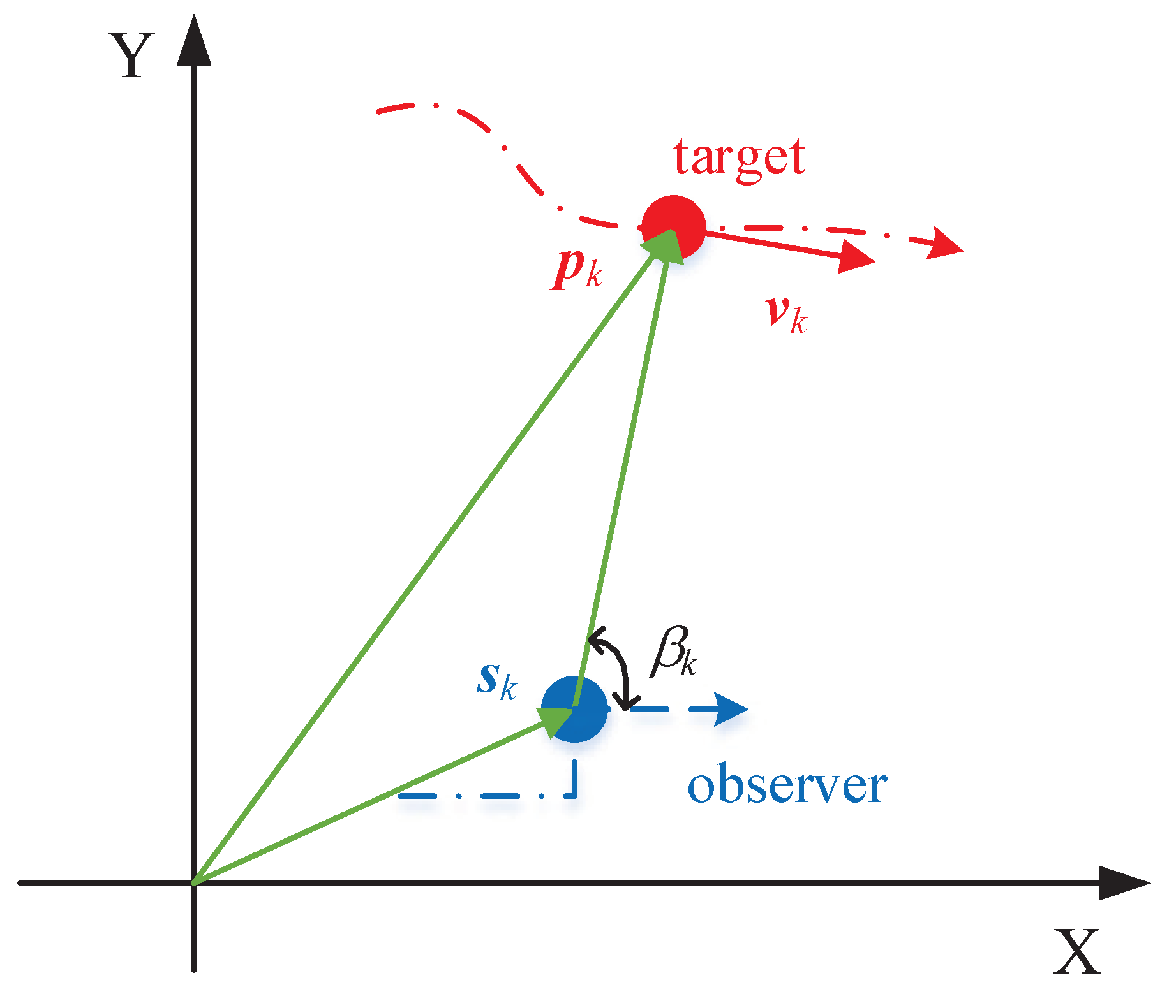
2.1. Problem Formulation

We focus on the BOT problem in 2D-plane with the bearing measurements received by a moving observer, which is shown in Figure 1. We denote by p k = [ p x , k , p y , k ] T R 2 × 1 and v k = [ v x , k , v y , k ] T R 2 × 1 the position and velocity of the target at the discrete time index k = 1 , , N , respectively. We then have target state vector x k = [ p k T , v k T ] T R 4 × 1 . The observer position is represented by the vector s k = [ s x , k , s y , k ] T R 2 × 1 , which is assumed to be known.
In the following, we assume that the target is moving under the constant velocity model as discussed in [32], then the target dynamic model is:
x k = F x k 1 + w k 1 ,
where F R 4 × 4 is the transition matrix, and w k 1 R 4 × 1 is the process noise, which is assumed to be a Gaussian random vector with mean 0 4 × 1 and covariance matrix Q R 4 × 4 . The matrices F and Q are given by [32]
F = 1 0 T 0 0 1 0 T 0 0 1 0 0 0 0 1 ,
Q = q x T 3 3 0 q x T 2 2 0 0 q y T 3 3 0 q y T 2 2 q x T 2 2 0 q x T 0 0 q y T 2 2 0 q y T ,
where T is the sample interval, which is assumed to be equal to 1 s throughout the paper. q x and q y are respectively the power spectral densities of w k in two coordinates.
We adopt β ˜ k to denote the bearing collected by the observer at k. It can be written as
β ˜ k = β k + n k ,
β k = tan 1 Δ y k Δ x k ,
where Δ x k = p x , k s x , k , Δ y k = p y , k s y , k , tan 1 is the four-quadrant inverse tangent function, and n k is the bearing noise, which is assumed to be Gaussian with zero mean and variance σ k 2 . σ k is assumed to be known, and n k is independent of the process noise w k throughout the paper.

2.2. Overview of the PLKF, BC–PLKF, and IV–PLKF

This subsection first discusses the PLKF algorithm and then analyses its bias. Afterwards, the improved PLKF algorithms–BC–PLKF and IV–PLKF in [25] are introduced.

2.2.1. PLKF

Obviously, we have the following equation:
sin n k = sin ( β ˜ k β k ) = sin β ˜ k cos β k cos β ˜ k sin β k ,
multiplying d k = Δ x k 2 + Δ y k 2 to both sides of (6), and notice that d k × cos β k = Δ x k , d k × sin β k = Δ y k , we have
d k sin n k = sin β ˜ k Δ x k cos β ˜ k Δ y k = sin β ˜ k ( p x , k s x , k ) cos β ˜ k ( p y , k s y , k ) = [ sin β ˜ k , cos β ˜ k ] p k [ sin β ˜ k , cos β ˜ k ] s k = [ sin β ˜ k , cos β ˜ k , 0 , 0 ] x k [ sin β ˜ k , cos β ˜ k ] s k .
Then we have the following pseudo-linear measurement equation:
z k = H k x k + η k ,
where z k = [ sin β ˜ k , cos β ˜ k ] s k , H k = [ sin β ˜ k , cos β ˜ k , 0 , 0 ] , and η k = d k sin n k is the pseudo-linear noise. The variance of η k is denoted by R k = E { η k 2 } = d k 2 · E { sin 2 n k } d k 2 σ k 2 for small bearing noise n k .
Combining (1) and (8), the PLKF is given by
step 1
Predicting the state:
x ^ k | k 1 = F x ^ k 1 | k 1 ;
step 2
Predicting the covariance matrix:
P k | k 1 = F P k 1 | k 1 F T + Q ;
step 3
Calculating the gain matrix:
K k = P k | k 1 H k T R k + H k P k | k 1 H k T 1 ;
step 4
Updating the state:
x ^ k | k = x ^ k | k 1 + K k ( z k H k x ^ k | k 1 ) ;
step 5
Updating the covariance matrix:
P k | k = ( I 4 × 4 K k H k ) P k | k 1 ,
where x ^ k | k 1 R 4 × 1 and P k | k 1 R 4 × 4 denote, respectively, the one-step prediction and the corresponding prediction error covariance matrix, and K k R 4 × 1 denotes the Kalman gain, and x ^ k | k R 4 × 1 and P k | k R 4 × 4 are, respectively, the posterior state estimate and corresponding estimation error covariance matrix. Since the true values of d k and R k are not available, the approximated values are used,
d ^ k = x ^ k | k 1 ( 1 : 2 ) s k ,
R ^ k = d ^ k 2 σ k 2 .

2.2.2. BC–PLKF

According to [25], the posterior bias e k = x ^ k | k x k of the PLKF can be written as:
e k = A k + B k + C k
where
A k = P k | k 1 1 + H k T R ^ k 1 H k 1 P k | k 1 1 F x ^ k 1 | k 1 x k 1 ,
B k = P k | k 1 1 + H k T R ^ k 1 H k 1 P k | k 1 1 w k 1 ,
C k = P k | k 1 1 + H k T R ^ k 1 H k 1 P k | k 1 1 H k T R ^ k 1 η k .
The first term A k propagates the error from the last time k 1 , and it is not the cause that leads to the biased estimate in PLKF. The second term B k propagates the bias from the correlation between H k and w k 1 . If we assume the process noise w k is relatively small, then B k can be ignored. When it comes to the third term C k , it propagates the bias from the correlation between H k and η k , which cannot be ignored since they all contain the bearing noise n k . Thus, we can have the conclusion that it is the correlation between the H k and η k that leads to the biased estimate, and if we can compensate the bias from C k , the bias in x ^ k | k can be reduced.
So the bias compensation can be achieved by
x ^ k | k P k | k 1 1 + H k T R ^ k 1 H k 1 P k | k 1 1 H k T R ^ k 1 η k .
However, the true value of C k cannot be obtained; we are supposed to replace it with its conditional expectation based on x ^ k | k , which can be formulated as: [25]
C ^ k = P k | k 1 1 + H k T R ^ k 1 H k 1 P k | k 1 1 E H k T R ^ k 1 η k | x ^ k | k = P k | k R ^ k 1 σ k 2 M T ( M x ^ k | k s k ) ,
where M = I 2 × 2 , 0 2 × 2 , and we use the formula P k | k = P k | k 1 1 + H k T R ^ k 1 H k 1 .
Finally, the BC–PLKF is summarized below [25]:
step 1
Predicting the state:
x ^ k | k 1 = F x ^ k 1 | k 1 BC ;
step 2
Predicting the covariance matrix:
P k | k 1 = F P k 1 | k 1 BC F T + Q ;
step 3
Calculating the gain matrix:
K k BC = P k | k 1 H k T R ^ k + H k P k | k 1 H k T 1 ;
step 4
Updating the state:
x ^ k | k = x ^ k | k 1 + K k BC ( z k H k x ^ k | k 1 ) ;
step 5
Updating the covariance matrix:
P k | k BC = ( I 4 × 4 K k BC H k ) P k | k 1 ;
step 6
Bias compensation:
x ^ k | k BC = x ^ k | k + P k | k BC R ^ k 1 σ k 2 M T ( M x ^ k | k s k ) .

2.2.3. IV–PLKF

Unlike the BC–PLKF, the IV–PLKF tries to construct a vector G k , which is chosen to be independent of η k , and at the same time is strongly correlated with H k . The optimal form of G k is the noise-free version of H k [25]:
G k opt = [ sin β k , cos β k ] M .
Since the true bearing measurement β k is unavailable, a suboptimal vector based upon the estimate β ^ k BC from BC–PLKF is chosen:
β ^ k BC = tan 1 x ^ k | k BC ( 2 ) s y , k x ^ k | k BC ( 1 ) s x , k ,
G k = sin β ^ k BC , cos β ^ k BC M .
The complete IV–PLKF algorithm is [25]:
step 1
Predicting the state:
x ^ k | k 1 = F x ^ k 1 | k 1 IV ;
step 2
Predicting the covariance matrix:
P k | k 1 = F P k 1 | k 1 IV F T + Q ;
step 3
Calculating the gain matrix:
K k = P k | k 1 H k T R ^ k + H k P k | k 1 H k T 1 ;
step 4
Updating the state:
x ^ k | k = x ^ k | k 1 + K k ( z k H k x ^ k | k 1 ) ;
step 5
Updating the covariance matrix:
P k | k = ( I 4 × 4 K k H k ) P k | k 1 ;
step 6
Bias compensation:
x ^ k | k BC = x ^ k | k + P k | k R ^ k 1 σ k 2 M T ( M x ^ k | k s k ) ;
step 7
IV estimation:
G k = [ sin β ^ k BC , cos β ^ k BC ] M
K k IV = P k | k 1 G k T R ^ k + H k P k | k 1 G k T 1
x ^ k | k IV = x ^ k | k 1 + K k IV ( z k H k x ^ k | k 1 )
P k | k IV = P k | k 1 K k IV H k P k | k 1 .
We shall notice that, although the asymptotic convergence of the IV based method is verified in [26], the performance of the IV–PLKF is still limited by the BC–PLKF due to the usage of x ^ k | k BC in calculating β ^ k BC . When the BC–PLKF performance deteriorates in the manoeuvring scenario, the IV–PLKF will also suffer.

2.3. The Proposed UB–PLKF and VC–PLKF

We first propose the UB–PLKF to cope with the biased estimate problem in PLKF. Then we incorporate the velocity constraint information into the UB–PLKF to construct the VC–PLKF.

2.3.1. UB–PLKF

Revisiting the matrix H k in (8), we can rewrite it as follows:
H k = [ sin β ˜ k , cos β ˜ k , 0 , 0 ] = [ sin β k cos n k , cos β k cos n k , 0 , 0 ] + [ cos β k sin n k , sin β k sin n k , 0 , 0 ] [ sin β k , cos β k , 0 , 0 ] + n k [ cos β k , sin β k , 0 , 0 ] ,
where we assume cos n k 1 and sin n k n k for small bearing noise.
Substituting (41) into (8), we get:
z k [ sin β k , cos β k , 0 , 0 ] x k + n k cos β k , sin β k , 0 , 0 x k d k ;
here we also assume that η k = d k sin n k d k n k . Let m k = [ cos β k , sin β k , 0 , 0 ] x k d k , and multiplying 1 / m k to both sides of (42), we have:
z ¯ k = H ¯ k x k + n k ,
where z ¯ k = z k / m k , H ¯ k = [ sin β k , cos β k , 0 , 0 ] / m k . Notice that in (43), the measurement vector is independent of the noise, and the noise here is the bearing noise n k , not the pseudo-linear noise η k .
Based on (43), the expectation of C k is
E { C k } = E P k | k 1 1 + H ¯ k T σ k 2 H ¯ k 1 E H ¯ k T σ k 2 n k .
It is clear that (44) equals 0 because H ¯ k is no longer correlated with n k . Then, an unbiased PLKF algorithm is obtained as follows:
step 1
Predicting the state:
x ^ k | k 1 = F x ^ k 1 | k 1 UB ;
step 2
Predicting the covariance matrix:
P k | k 1 = F P k 1 | k 1 UB F T + Q ;
step 3
Calculating the gain matrix:
K k UB = P k | k 1 H ¯ k T σ k 2 + H ¯ k P k | k 1 H ¯ k T 1 ;
step 4
Updating the state:
x ^ k | k UB = x ^ k | k 1 + K k UB ( z ¯ k H ¯ k x ^ k | k 1 ) ;
step 5
Updating the covariance matrix:
P k | k UB = ( I 4 × 4 K k UB H ¯ k ) P k | k 1 .
Obviously, the true values of the bearing β k and m k in (43) cannot be obtained, we replace them with corresponding approximated versions β ^ k UB and m ^ k , which are defined as follows:
β ^ k UB = tan 1 x ^ k | k 1 ( 2 ) s y , k x ^ k | k 1 ( 1 ) s x , k ,
m ^ k = cos β ^ k UB , sin β ^ k UB , 0 , 0 x ^ k | k 1 d ^ k UB ,
d ^ k UB = x ^ k | k 1 ( 1 : 2 ) s k .
We emphasise here that the main idea behind the IV–PLKF and the UB–PLKF is similar. They both try to construct a noise-free measurement vector. However, the IV–PLKF performance is limited by the BC–PLKF, while the UB–PLKF does not suffer from this. The advantages of the UB–PLKF will be verified in the simulation part.

2.3.2. VC–PLKF

Based on the UB–PLKF, we develop its velocity constrained version in this part. First, we shall handle an optimisation problem with an equality constraint. Let v k | k = x ^ k | k UB (3:4) and e v , k = v k v k | k , we have:
min K v , k E { e v , k T e v , k } s · t · v k | k = v ,
where K k UB = K p , k T , K v , k T T , and K v , k R 2 × 1 . v is the velocity constraint, which is a positive constant. Note that E { e v , k T e v , k } = t r { P v v , k + } , and P k | k UB = P p p , k + P p v , k + P v p , k + P v v , k + . Then (53) can be rewritten as
min K v , k t r { P v v , k + } s · t · v k | k = v .
Let v k | k 1 = x ^ k | k 1 (3:4) in (45), and according to the Kalman formula, we have:
v k | k = v k | k 1 + K v , k ϵ k ,
where ϵ k = z ¯ k H ¯ k x ^ k | k 1 UB . Substituting (55) into the velocity constraint in (54), we have:
ϵ k 2 K v , k T K v , k + 2 v k | k 1 T K v , k ϵ k + v k | k 1 T v k | k 1 v 2 = 0 .
According to the Joseph formula [33], the update formula of the partitioned p o s t e r i o r covariance matrix can be written as:
P v v , k + = P v v , k K v , k H ¯ k P 2 , k P 2 , k T H ¯ k T K v , k T + K v , k W k K v , k T ,
where
P k | k 1 = P 1 , k , P 2 , k = P p p , k P p v , k P v p , k P v v , k
and
W k = H ¯ k P k | k 1 H ¯ k T + σ k 2 .
Utilising (56) and (57) and the Lagrange multiplier method, we can construct the performance index j k as follows:
j k = t r P v v , k K v , k H ¯ k P 2 , k P 2 , k T H ¯ k T K v , k T + K v , k W k K v , k T + λ k ϵ k 2 K v , k T K v , k + 2 v k | k 1 T K v , k ϵ k + v k | k 1 T v k | k 1 v 2 .
Taking the first derivative of j k with respect to K v , k and setting it to zero yields:
P 2 , k T H ¯ k T + K v , k W k + λ k ( v k | k 1 ϵ k + K v , k ϵ k 2 ) = 0 .
Then we have the first-order condition:
K v , k = P 2 , k T H ¯ k T λ k v k | k 1 ϵ k W k + λ k ϵ k 2 .
Substituting (62) into (56), and according to [27], the scalar equation with λ k can be obtained as:
λ k 2 ϵ ˜ k 2 v 2 2 λ k ϵ ˜ k v 2 + ϵ k 2 H ¯ k P 2 , k P 2 , k T H ¯ k T W k 2 + 2 v k | k 1 T P 2 , k T H ¯ k T ϵ k W k + v k | k 1 T v k | k 1 v 2 = 0 ,
where ϵ ˜ k = ϵ k 2 / W k .
Then, λ k can be written as
λ k = b b 2 4 a c 2 a ,
where
a = v 2 ϵ ˜ k 2 ,
b = 2 ϵ ˜ k v 2 ,
c = ϵ k 2 H ¯ k P 2 , k P 2 , k T H ¯ k T / W k 2 + 2 v k | k 1 T P 2 , k T H ¯ k T ϵ k / W k + v k | k 1 T v k | k 1 v 2 .
Notice that we use b b 2 4 a c , not b ± b 2 4 a c , because the minimum performance index j k occurs when the minus sign is chosen according to [27].
Substituting (64)–(67) into (62) we get:
K v , k * = K v , k + v v k | k 1 v k | k ϵ k ,
where the asterisk was added to distinguish from the unconstrained form K v , k . (see Appendix A).
Now we have the VC–PLKF with an equality constraint as follows:
step 1
Predicting the state:
x ^ k | k 1 = F x ^ k 1 | k 1 VC ;
step 2
Predicting the covariance matrix:
P k | k 1 = F P k 1 | k 1 VC F T + Q ;
step 3
Calculating the gain matrix for UB–PLKF:
K k UB = P k | k 1 H ¯ k T / σ k 2 + H ¯ k P k | k 1 H ¯ k T ;
step 4
Calculating the innovation:
ϵ k = z ¯ k H ¯ k x ^ k | k 1 ;
step 5
Updating the state:
x ^ k | k UB = x ^ k | k 1 + K k UB ϵ k ;
step 6
Updating the covariance for UB–PLKF:
P k | k UB = ( I 4 × 4 K k UB H ¯ k ) P k | k 1 ;
step 7
Constructing the VC–PLKF:
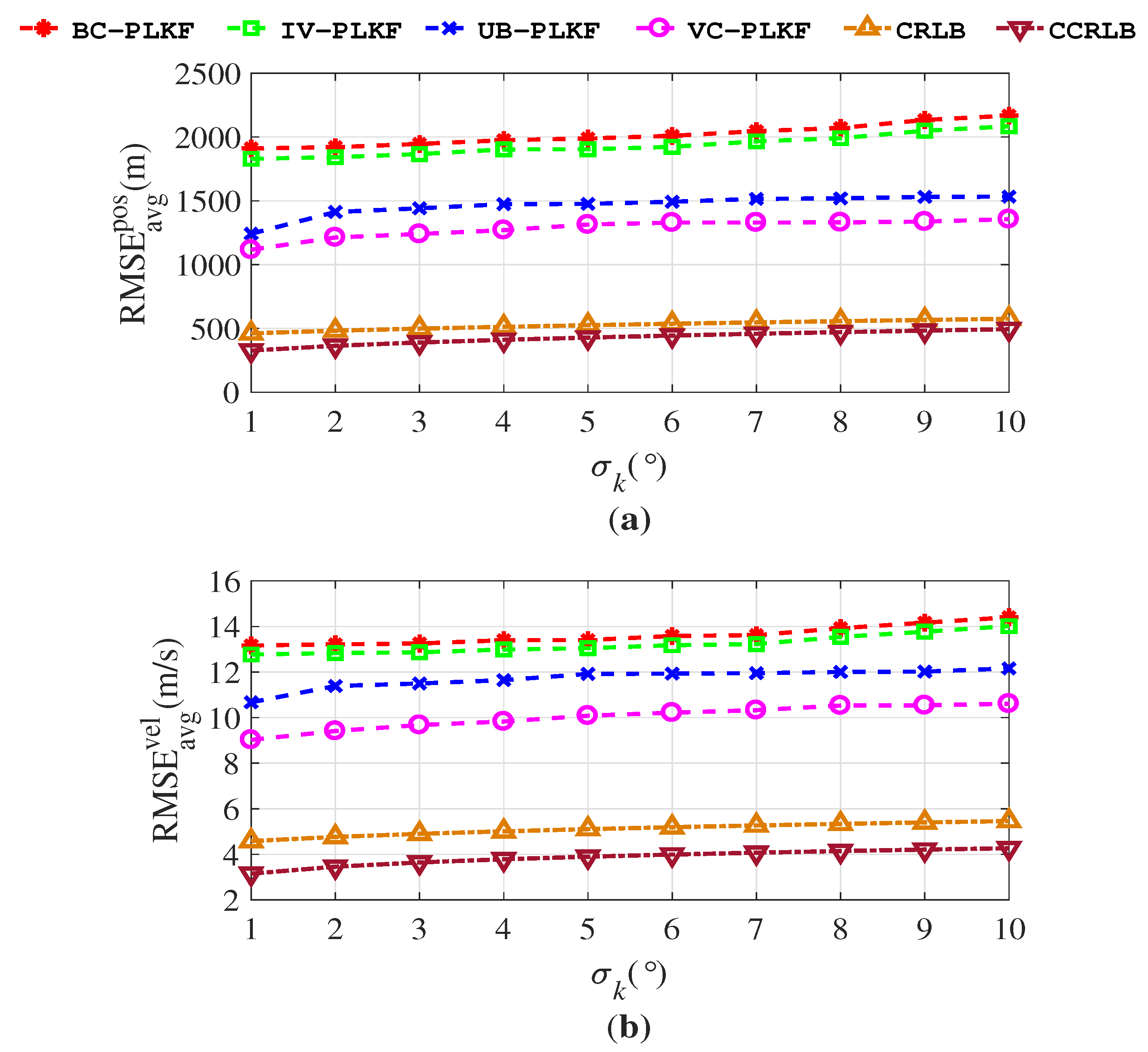
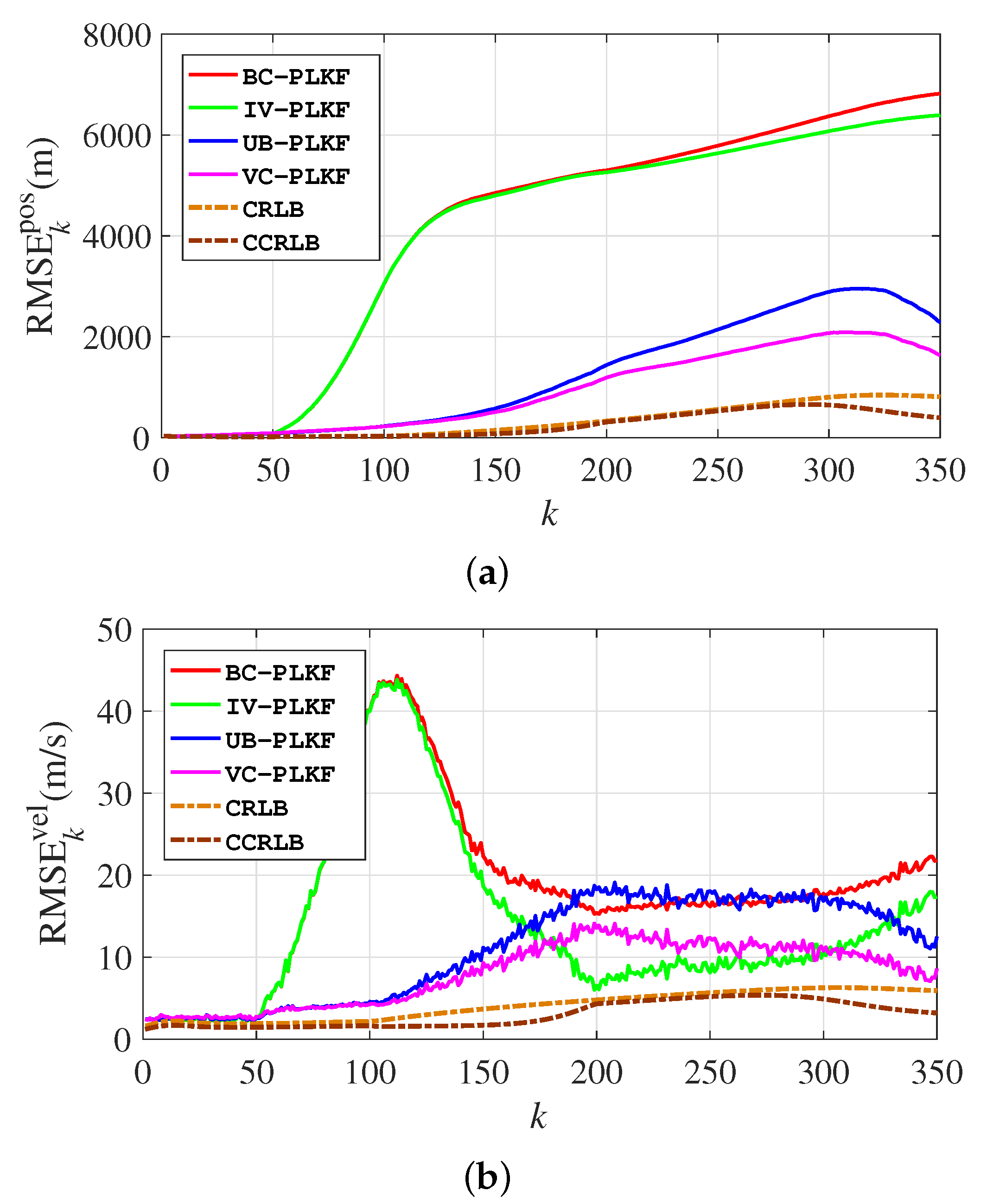
v k | k = x ^ k | k UB ( 3 : 4 )
K v , k * = K k UB ( 3 : 4 ) + v v k | k 1 v k | k ϵ k
K k VC = K k UB ( 1 : 2 ) ; K v , k *
x ^ k | k VC = x ^ k | k 1 + K k VC ϵ k
P k | k VC = ( I 4 × 4 K k VC H ¯ k ) P k | k 1 .
In most cases, however, what we know is the target velocity range, and this means we should handle a problem with inequality constraints. To translate the inequality constraint into the equality constraint, we adopt the rule in [29], that is,
x ^ k | k VC = x ^ k | k VC v = v max if v k | k > v max , x ^ k | k VC v = v min if v k | k < v min , x ^ k | k VC = x ^ k | k UB if v min v k | k v max .
Here, v min and v max denote the lower and upper bounds of the velocity, respectively. Equation (80) means that if v k | k [ v min , v max ] , the steps after (75) are avoided, and we just output x ^ k | k VC = x ^ k | k UB and P k | k VC = P k | k UB . Otherwise, if v k | k is less than v min or greater than v max , we do the VC–PLKF with the equality constraint with v = v min or v = v max , respectively.
We shall emphasise that, although the VC–PLKF and the algorithms in [29] all make use of the velocity constraints, the VC–PLKF constructs a norm-constrained Kalman filter, which is an iterative algorithm; however, algorithms in [29] are all based on the batch algorithms, which are computationally expensive and can hardly handle the manoeuvring target tracking problem.

3. Results

In this section, the proposed UB–PLKF and VC–PLKF are compared with the BC–PLKF and the IV–PLKF via Monte Carlo (MC) simulations. We adopt the root mean square error (RMSE) and the time-averaged RMSE as the performance metrics.
Assuming that x ^ k | k i is the state vector that we estimate at k via i th MC simulation. We can define the RMSEs obtained from M = 300 MC simulations as follows:
RMSE k pos = 1 M i = 1 M p ^ k | k i p k 2 1 / 2
RMSE k vel = 1 M i = 1 M v ^ k | k i v k 2 1 / 2
where p ^ k | k i = x ^ k | k i ( 1 : 2 ) , v ^ k | k i = x ^ k | k i (3:4).
The time-averaged RMSEs are also adopted and are computed as [25]:
RMSE avg pos = 1 M U i = 1 M k = P N p ^ k | k i p k 2 1 / 2
RMSE avg vel = 1 M U i = 1 M k = P N v ^ k | k i v k 2 1 / 2 ,
where U = N P + 1 is the effective time that takes into account the computation of time-averaged RMSEs, N = 350 is the total number of time index k, and P = 60 is chosen to eliminate the influence of the initial error according to [25].

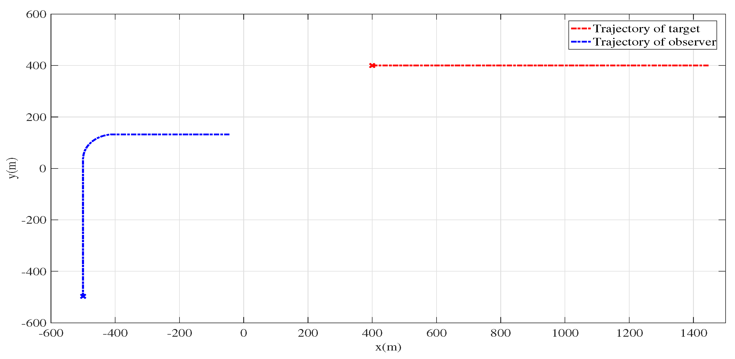
3.1. Scenario 1: Non-Manoeuvring Target Tracking

We first test the filters’ performance against poor initialisation and poor target sensor geometry with a non-manoeuvring scenario, which is given in Figure 2. The initial state vector of the target is x 0 = [ 400 , 400 , 3 , 0 ] T , and to test the performance against poor initialisation, we set the initial state of the estimate x ^ 0 | 1 Gaussian, and its mean is [ 500 , 300 , 2 , 1 ] T and the covariance matrix is P 0 | 1 = diag ( 625 , 625 , 4 , 4 ) . The observer starts at [ 500 , 500 ] T m and follows a linear path with a constant speed of [ 0 , 3 ] T m / s for the first 180 scans. Then, it executes a coordinated turn for 50 scans with a turn rate of 1.8 / s followed by 120 scans, where it moves in a straight line with velocity [ 3 , 0 ] T m / s . Notice that at the last 120 scans, the bearing rate between the target and the observer is 0, which constructs the case of poor target sensor geometry. q x and q y in (3) are q x = q y = 0.2 m 2 / s 3 . The standard deviation σ k = 5 is assumed to be time invariant. The upper bound of the velocity is v max = 6 m / s , while the lower bound is v min = 1 m / s .
Figure 3 shows the RMSEs for different algorithms. The IV–PLKF and BC–PLKF show similar performances in RMSEs of both the position and velocity, and so do the UB–PLKF and VC–PLKF. However, the biases of the UB–PLKF and VC–PLKF are much smaller than the BC–PLKF and IV–PLKFs, and this suggests that splitting the noise n k away from the H k is more effective than subtracting the bias from PLKF. Divergence problems have not been present in RMSEs of UB–PLKF and VC–PLKF, and this suggests that the proposed UB–PLKF and VC–PLKF can work well in conditions of poor initialisation and poor target sensor geometry.

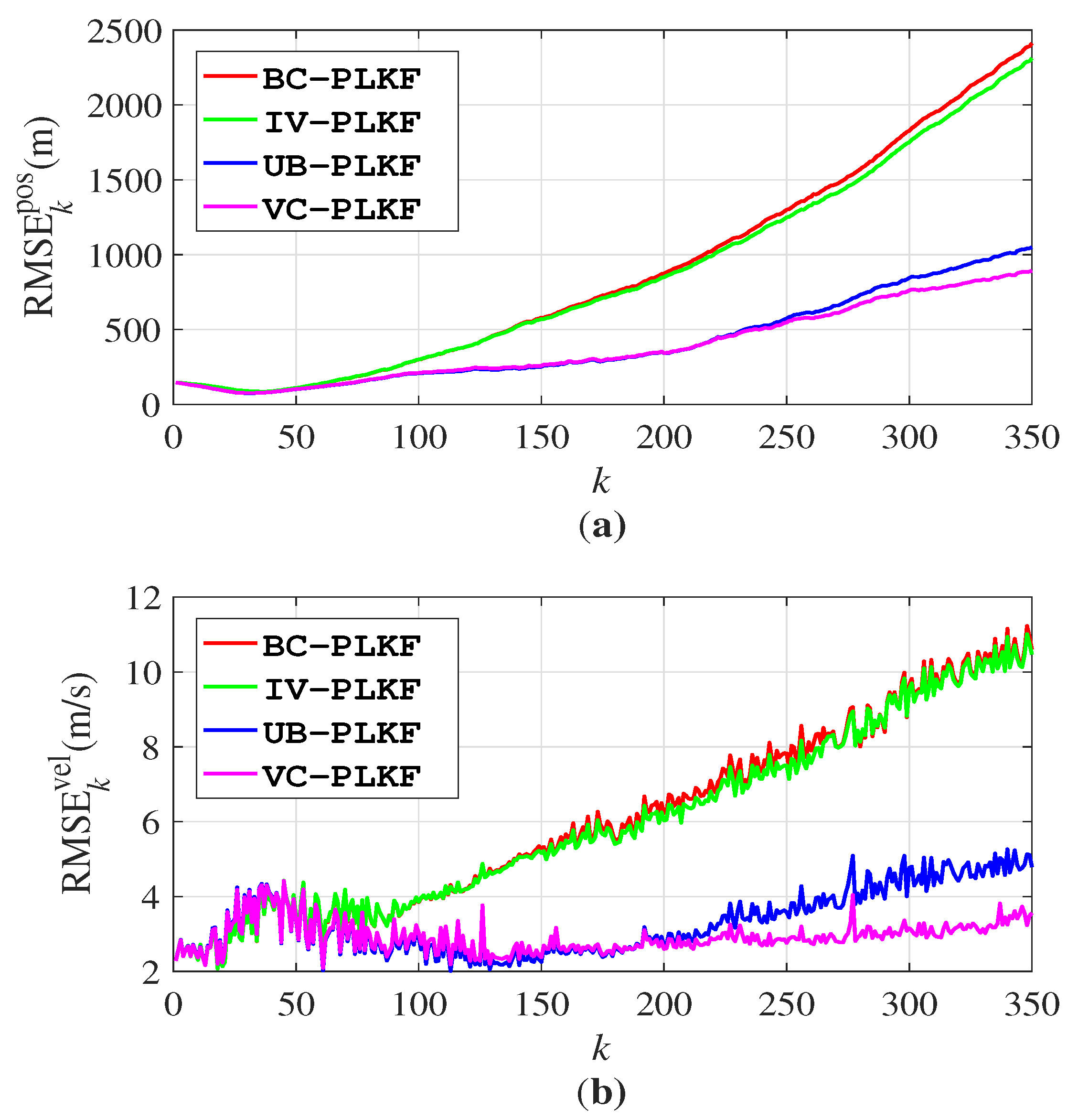
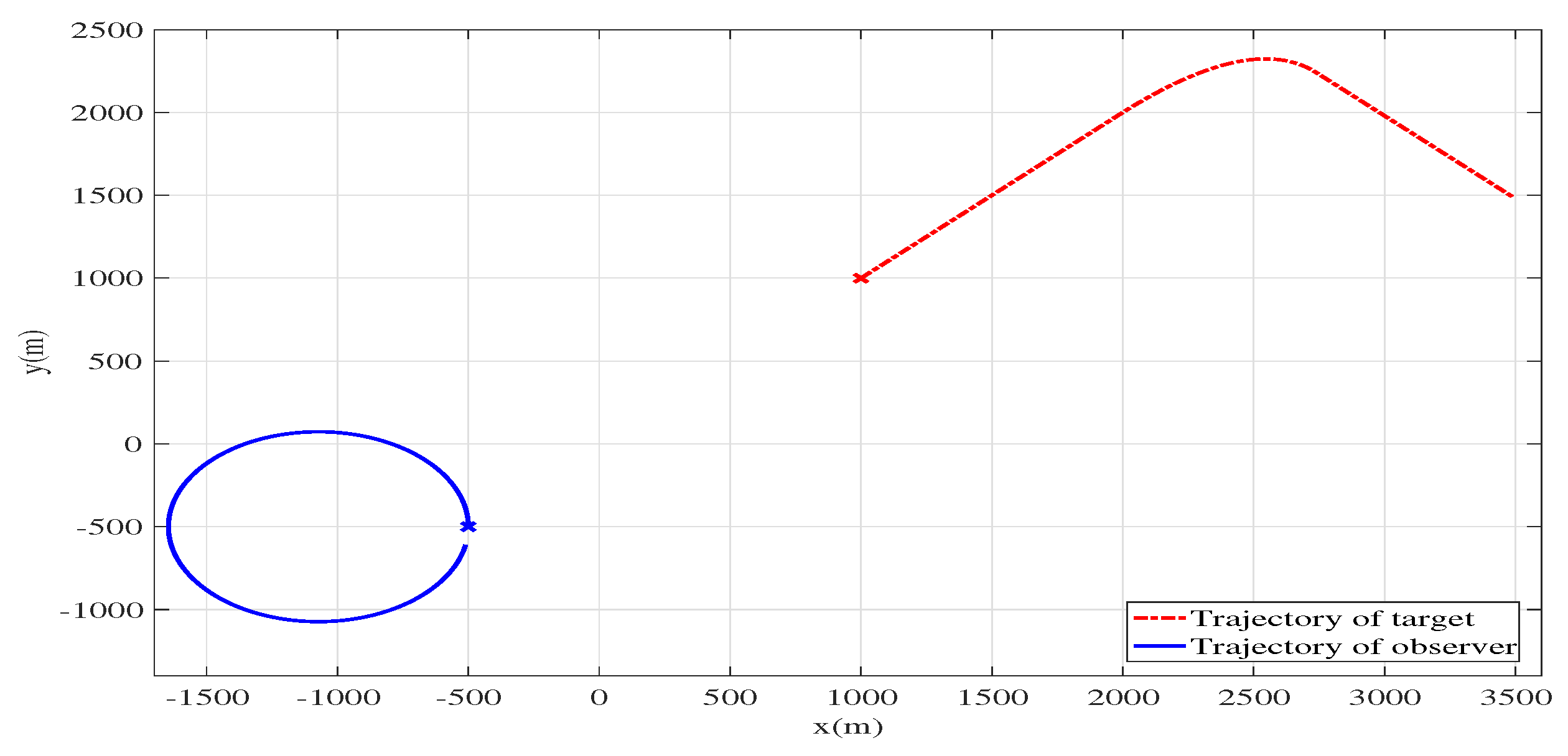
3.2. Scenario 2: Manoeuvring Target Tracking

Figure 4 represents the geometry of scenario 2. The initial state of the target is x 0 = [ 1000 , 1000 , 10 , 10 ] T , and it moves in a straight line for the first 100 scans. Then it performs a constant acceleration movement [32] with acceleration [ 0.05 , 0.15 ] T m / s 2 in the following 100 scans. In the final 150 scans, it moves along a straight line at a constant speed [ 5 , 5 ] T m / s . The initial state of the estimate x ^ 0 | 1 is a Gaussian random vector with mean [ 1000 , 1000 , 10 , 10 ] T , and the rest of the settings are the same as those of scenario 1, except that v min = 5 m / s and v max = 16 m / s . The observer begins at [ 500 , 500 ] T m with velocity [ 0 , 9.45 ] T m / s , and executes a coordinated turn for the whole 350 scans with a turn rate of 1.8 / s , where “−” means the anticlockwise direction. We also adopt the Cramer–Rao lower bound (CRLB) [34] and the constrained Cramer–Rao lower bound (CCRLB) [35] in this scenario to evaluate the performance of the four algorithms (the derivation of CRLB and CCRLB can be found in Appendix B).
Figure 5 plots the RMSEs and CRLB for the four algorithms. The RMSEs of the VC–PLKF are closest to the CRLB and CCRLB, followed by UB–PLKF. We also find that the velocity RMSEs of UB–PLKF and VC–PLKF decrease after the manoeuvring, which means that the proposed algorithms are more adaptable to abrupt changes in the velocity. Figure 6 shows the time-averaged RMSEs for σ k { 1 , , 10 } ; it also verifies that the VC–PLKF and UB–PLKF outperform the BC–PLKF and IV–PLKF. The time-averaged RMSEs of the four algorithms are also flat, which proves that the four algorithms all have good robustness to the different levels of the bearing noise.
To test the performance of the proposed algorithms in the case in which there exists a noise statistics mismatch, we again assume that the deviation σ k is time-varying. When k < 51 or k > 201 , σ k = 3 , whereas σ k = 7 at the other times. The other settings remain unchanged. Figure 7 shows the RMSEs of different algorithms. It is clear that the position RMSEs of the BC–PLKF and IV–PLKF get worse when the mismatch begins, and retain high levels the rest of the time. However, the mismatch has little influence on the proposed UB–PLKF and VC–PLKF. The shapes of their positions and velocity RMSE curves are basically the same as those in Figure 5. This verifies that the UB–PLKF and VC–PLKF are more robust to the noise statistics mismatch. When it comes to the velocity RMSEs, some differences may occur. We can find that, although the velocity RMSEs of the IV–PLKF gets worse after the mismatch begins, it becomes smaller after the 100th scan. The possible reason is that at the 100th scan, the target starts to manoeuvre, and at this time, large measurement errors occur. So the large variance may more adaptable to this case. However, after the 201st scan, the velocity RMSEs of the BC–PLKF and IV–PLKF get worse again and finally exceed the RMSEs of UB–PLKF and VC–PLKF.
Table 1 lists four different cases of velocity constraints to compare the influence of different constraints in VC–PLKF. The time-averaged RMSEs are given by Figure 8. The closer the constraint is to the true speed, the smaller the RMSE of the VC–PLKF is. However, this improvement is at the cost of reducing the application scope of the algorithm. Thus, the choices of the upper and lower bounds depend on our prior knowledge of the target, otherwise it is suggested to choose a large range of constraints.

4. Discussion

Section 3 compares the algorithms’ performances in terms of RMSE and time-averaged RMSE. Figure 3 and Figure 5 show that the proposed algorithms outperform the BC–PLKF and IV–PLKF in [25] both in non-manoeuvring and manoeuvring scenarios. This is not surprising since the BC–PLKF just subtracts the approximated bias and does not split the noise away from the H k . When the target manoeuvres or the target sensor geometry becomes poor, the approximated bias may not be accurate, which leads to huge biases in BC–PLKF. The IV–PLKF also suffers from this, since it utilizes the results of the BC–PLKF to calculate the approximated bearings. However, the proposed algorithms are unbiased and can be rapidly adapted to the changes in the scenarios.
Table 2 records the runtimes of the four algorithms, which are normalised by the UB–PLKF runtime. It shows that the UB–PLKF costs the least time among the four improved algorithms because it avoids the bias compensation step in BC–PLKF. The VC–PLKF and BC–PLKF have similar complexity, while the IV–PLKF takes the longest time to run. Considering the RMSEs, the time-averaged RMSEs and the runtimes, we can draw the conclusion that the proposed UB–PLKF and VC–PLKF outperform the BC–PLKF and IV–PLKF, both in terms of tracking accuracy and real-time application.
In this paper, we assume that the statistical characteristics of noise are known a priori; however, this is not true in practical application. So, future research may contain the construction of the UB–PLKF in terms of the unknown statistical characteristics of noise by variational inference [36].

5. Conclusions

To handle the bias problem in the traditional PLKF algorithm, we propose the UB–PLKF algorithm. Unlike the existing BC–PLKF and IV–PLKF, the UB–PLKF splits the noise away from the measurement vector directly, which can lead to an unbiased estimate. We then develop the VC–PLKF by solving a partial norm-constrained optimisation problem with an inequality relation to improve the performance of UB–PLKF. Simulation results show that the UB–PLKF and VC–PLKF outperform the BC–PLKF and IV–PLKF according to the RMSE, the time-averaged RMSE, and the computational complexity. The results also verify that the proposed algorithms can adapt to the abrupt changes of the target velocity, and thus are more suitable for the manoeuvring target tracking scenario.

Author Contributions

Conceptualization, Z.H.; methodology, Z.H.; software, Z.H. and S.C.; validation, C.H. and D.O.; formal analysis, Z.H.; investigation, Z.H. and S.C.; writing—original draft preparation, Z.H.; funding acquisition, C.H.; writing—review and editing, C.H. and D.O. All authors have read and agreed to the published version of the manuscript.

Funding

This research is founded by the National Natural Science Foundation of China under Grant No. 61971412.

Institutional Review Board Statement

Not applicable.

Informed Consent Statement

Not applicable.

Data Availability Statement

Not applicable.

Conflicts of Interest

The authors declare no conflict of interest.

Appendix A

Substituting (65)–(67) into (64), the polynomial b 2 4 a c can be written as
b 2 4 a c = 4 ϵ ˜ k 2 v 4 + 4 v 2 ϵ ˜ k 2 ϵ k 2 H ¯ k P 2 , k P 2 , k T H ¯ k T / W k 2 4 v 4 ϵ ˜ k 2 + 8 v 2 ϵ ˜ k 2 v k | k 1 T P 2 , k T H ¯ k T ϵ k / W k + 4 v 2 ϵ ˜ k 2 v k | k 1 T v k | k 1 = 4 v 2 ϵ ˜ k 2 ϵ k P 2 , k T H ¯ k T / W k + v k | k 1 2 = 4 v 2 ϵ ˜ k 2 v k | k 2 .
Thus λ k in (64) can be written as
λ k = 1 ϵ ˜ k + v k | k ϵ ˜ k v .
Substituting (A2) into (62), we have
K v , k * = P 2 , k T H ¯ k T + v v k | k v ϵ ˜ k v k | k 1 ϵ k W k + λ k ϵ k 2 1 = P 2 , k T H ¯ k T + v v k | k v ϵ ˜ k v k | k 1 ϵ k v v k | k W k = v P 2 , k T H ¯ k T W k v k | k I + v ϵ k v k | k 1 ϵ ˜ k v k | k W k II ϵ k v k | k 1 ϵ ˜ k W k III .
Note that in part I: P 2 , k T H ¯ k T / W k = K v , k , and in part II and III: ϵ k / ( ϵ ˜ k W k ) = 1 / ϵ k , (A3) can be further written as
K v , k * = v v k | k K v , k + v k | k 1 v ϵ k v k | k v k | k 1 ϵ k = v v k | k K v , k + v v k | k 1 v k | k 1 ϵ k = v v k | k K v , k + v v k | k 1 v k | k K v , k ϵ k ϵ k = K v , k + v v k | k 1 v k | k ϵ k .

Appendix B

According to [34], an elegant way to calculate the Fisher information matrix (FIM) J k recursively can be written as
J k + 1 = D k 22 D k 21 J k + D k 11 1 D k 12
where
D k 11 = E Δ x k x k lg p x k + 1 | x k
D k 12 = E Δ x k x k + 1 lg p x k + 1 | x k
D k 21 = D k 12 T ,
and
D k 22 = E Δ x k + 1 x k + 1 lg p x k + 1 | x k + E Δ x k + 1 x k + 1 lg p z ¯ k + 1 | x k + 1 .
Here p x k + 1 | x k and p z ¯ k + 1 | x k + 1 are the transition and measurement probability density functions, and Δ Φ Ψ is the second-order partial derivative operators.
Based on (1) and (43), we have D k 11 = F T Q 1 F , D k 12 = F T Q 1 , D k 21 = Q 1 F , and D k 22 = Q 1 + H ¯ k + 1 T H ¯ k + 1 / σ k + 1 2 . The initial state of J 0 is chosen to be P 0 | 1 .
When it comes to the constrained Cramer-Rao lower bound, its FIM J C , k can be calculated as [35]
J C , k 1 = J k 1 J k 1 U k T U k J k 1 U k T 1 U k J k 1
where U k is the gradient matrix which is defined by
U k = A x k 2 x k T = 2 x k T A T A
where A = [ 0 2 × 2 , I 2 × 2 ] .
Finally, according to the relationship between the FIM and Cramer-Rao lower bound J k 1 CRLB , we can calculate the CRLB and CCRLB recursively.

References

  1. Lingren, A.G.; Gong, K.F. Position and Velocity Estimation Via Bearing Observations. IEEE Trans. Aerosp. Electron. Syst. 1978, AES-14, 564–577. [Google Scholar] [CrossRef]
  2. Nardone, S.; Lindgren, A.; Gong, K. Fundamental properties and performance of conventional bearings-only target motion analysis. IEEE Trans. Autom. Control 1984, 29, 775–787. [Google Scholar] [CrossRef]
  3. Jagan, B.O.L.; Rao, S.K. Underwater surveillance in non-Gaussian noisy environment. Meas. Control 2020, 53, 250–261. [Google Scholar] [CrossRef] [Green Version]
  4. Xu, S.; Doğançay, K.; Hmam, H. 3D AOA target tracking using distributed sensors with multi-hop information sharing. Signal Process. 2018, 144, 192–200. [Google Scholar] [CrossRef]
  5. Su, J.; Li, Y.A.; Ali, W. Underwater angle-only tracking with propagation delay and time-offset between observers. Signal Process. 2020, 176, 107581. [Google Scholar] [CrossRef]
  6. Modalavalasa, N.; Rao, G.S.B.; Prasad, K.S.; Ganesh, L.; Kumar, M.N.V.S.S. A new method of target tracking by EKF using bearing and elevation measurements for underwater environment. Robot. Auton. Syst. 2015, 74, 221–228. [Google Scholar] [CrossRef]
  7. Liu, B.; Tang, X.; Tharmarasa, R.; Kirubarajan, T.; Jassemi, R.; Halle, S. Underwater Target Tracking in Uncertain Multipath Ocean Environments. IEEE Trans. Aerosp. Electron. Syst. 2020, 56, 4899–4915. [Google Scholar] [CrossRef]
  8. Xu, S.; Doğançay, K.; Hmam, H. Distributed pseudolinear estimation and UAV path optimization for 3D AOA target tracking. Signal Process. 2017, 133, 64–78. [Google Scholar] [CrossRef]
  9. He, L.; Gong, P.; Zhang, X.; Wang, Z. The Bearing-Only Target localization via the Single UAV: Asymptotically Unbiased Closed-Form Solution and Path Planning. IEEE Access 2019, 7, 153592–153604. [Google Scholar] [CrossRef]
  10. Rutkowski, A.; Kawalec, A. Some of Problems of Direction Finding of Ground-Based Radars Using Monopulse Location System Installed on Unmanned Aerial Vehicle. Sensors 2018, 20, 5186. [Google Scholar] [CrossRef]
  11. Liao, S.L.; Zhu, R.M.; Wu, N.Q.; Shaikh, T.A.; Sharaf, M.; Mostafa, A.M. Path planning for moving target tracking by fixed-wing UAV. Def. Technol. 2019, 16, 811–824. [Google Scholar] [CrossRef]
  12. Pham, D.T. Some quick and efficient methods for bearing-only target motion analysis. IEEE Trans. Signal Process. 1993, 41, 2737–2751. [Google Scholar] [CrossRef]
  13. Aidala, V.; Hammel, S. Utilization of modified polar coordinates for bearings-only tracking. IEEE Trans. Autom. Control 1983, 28, 283–294. [Google Scholar] [CrossRef] [Green Version]
  14. Kim, J.; Suh, T.; Ryu, J. Bearings-only target motion analysis of a highly manoeuvring target. IET Radar Sonar Navig. 2017, 11, 1011–1019. [Google Scholar] [CrossRef]
  15. Julier, S.; Uhlmann, J.; Durrant-Whyte, H.F. A new method for the nonlinear transformation of means and covariances in filters and estimators. IEEE Trans. Autom. Control 2000, 45, 477–482. [Google Scholar] [CrossRef] [Green Version]
  16. Arasaratnam, I.; Haykin, S. Cubature Kalman Filters. IEEE Trans. Autom. Control 2009, 54, 1254–1269. [Google Scholar] [CrossRef] [Green Version]
  17. Toloei, A.; Niazi, S. State Estimation for Target Tracking Problems with Nonlinear Kalman Filter Algorithms. Int. J. Comput. Appl. 2014, 98, 30–36. [Google Scholar] [CrossRef]
  18. Wu, H.; Chen, S.; Yang, B.; Chen, K. Robust Derivative-Free Cubature Kalman Filter for Bearings-Only Tracking. J. Guid. Control Dyn. 2016, 39, 1865–1870. [Google Scholar] [CrossRef]
  19. Ristic, B.; Houssineau, J.; Arulampalam, S. Robust target motion analysis using the possibility particle filter. IET Radar Sonar Navig. 2018, 13, 18–22. [Google Scholar] [CrossRef]
  20. Zhang, H.W.; Xie, W.X. Constrained auxiliary particle filtering for bearings-only maneuvering target tracking. J. Syst. Eng. Electron. 2019, 30, 684–695. [Google Scholar] [CrossRef] [Green Version]
  21. Ayham, Z.; Thomas, S.; Shannon, D.A. Optimal Shadowing Filter for a Positioning and Tracking Methodology with Limited Information. Sensors 2019, 19, 931. [Google Scholar] [CrossRef] [Green Version]
  22. Thomas, S.; Kevin, J. A guide to using shadowing filters for forecasting and state estimation. Physica D 2009, 238, 1260–1273. [Google Scholar] [CrossRef]
  23. Aidala, V.J. Kalman Filter Behavior in Bearings-Only Tracking Applications. IEEE Trans. Aerosp. Electron. Syst. 1979, AES-15, 29–39. [Google Scholar] [CrossRef]
  24. Lin, X.; Kirubarajan, T.; Bar-Shalom, Y.; Maskell, S. Comparison of EKF, pseudomeasurement, and particle filters for a bearing-only target tracking problem. In Proceedings of the Signal and Data Processing of Small Targets 2002, Orlando, FL, USA, 2–4 April 2002; International Society for Optics and Photonics: Bellingham, WA, USA, 2002; Volume 4728, pp. 240–250. [Google Scholar] [CrossRef]
  25. Nguyen, N.H.; Doğançay, K. Improved Pseudolinear Kalman Filter Algorithms for Bearings-Only Target Tracking. IEEE Trans. Signal Process. 2017, 65, 6119–6134. [Google Scholar] [CrossRef]
  26. Zhang, Y.J.; Xu, G.Z. Bearings-Only Target Motion Analysis via Instrumental Variable Estimation. IEEE Trans. Signal Process. 2010, 58, 5523–5533. [Google Scholar] [CrossRef]
  27. Zanetti, R.; Majji, M.; Bishop, R.H.; Mortari, D. Norm-Constrained Kalman Filtering. J. Guid. Control Dyn. 2009, 32, 1458–1465. [Google Scholar] [CrossRef]
  28. Simon, D. Kalman filtering with state constraints: A survey of linear and nonlinear algorithms. IET Control Theory Appl. 2010, 4, 1303–1318. [Google Scholar] [CrossRef] [Green Version]
  29. Badriasl, L.; Arulampalam, S.; van der Hoek, J.; Finn, A. Bayesian WIV Estimators for 3-D Bearings-Only TMA With Speed Constraints. IEEE Trans. Signal Process. 2019, 67, 3576–3591. [Google Scholar] [CrossRef]
  30. He, S.M.; Shin, H.S.; Tsourdos, A. Trajectory Optimization for Target Localization With Bearing-Only Measurement. IEEE Trans. Robot. 2019, 35, 653–668. [Google Scholar] [CrossRef] [Green Version]
  31. Kim, H.G.; Lee, J.Y.; Kim, H.J. Look Angle Constrained Impact Angle Control Guidance Law for Homing Missiles With Bearings-Only Measurements. IEEE Trans. Aerosp. Electron. Syst. 2018, 54, 3096–3107. [Google Scholar] [CrossRef]
  32. Rong Li, X.; Jilkov, V.P. Survey of maneuvering target tracking. Part I. Dynamic models. IEEE Trans. Aerosp. Electron. Syst. 2003, 39, 1333–1364. [Google Scholar] [CrossRef]
  33. Zanetti, R.; DeMars, K.J. Joseph Formulation of Unscented and Quadrature Filters with Application to Consider States. J. Guid. Control Dyn. 2013, 36, 1860–1864. [Google Scholar] [CrossRef] [Green Version]
  34. Schmitt, L.; Fichter, W. Globally Valid Posterior Cramer-Rao Bound for Three-Dimensional Bearings-Only Filtering. IEEE Trans. Aerosp. Electron. Syst. 2019, 55, 2036–2044. [Google Scholar] [CrossRef]
  35. Nitzan, E.; Routtenberg, T.; Tabrikian, J. Cramer-Rao Bound for Constrained Parameter Estimation Using Lehmann-Unbiasedness. IEEE Trans. Signal Process. 2019, 67, 753–768. [Google Scholar] [CrossRef] [Green Version]
  36. Sarkka, S.; Nummenmaa, A. Recursive Noise Adaptive Kalman Filtering by Variational Bayesian Approximations. IEEE Trans. Autom. Control 2009, 3, 596–600. [Google Scholar] [CrossRef]
Figure 1. Geometry for 2-D BOT problem.
Remotesensing 13 02915 g001
Figure 2. Geometry for scenario 1. The red curve represents the target trajectory while the observer trajectory is given by the blue curve.
Remotesensing 13 02915 g002
Figure 3. RMSEs for different algorithms in non-manoeuvring target tracking: (a) RMSEs for position; (b) RMSEs for velocity.
Remotesensing 13 02915 g003
Figure 4. Geometry for scenario 2. The red curve represents the target trajectory while the observer trajectory is given by the blue curve.
Remotesensing 13 02915 g004
Figure 5. RMSEs for different algorithms in manoeuvring target tracking: (a) RMSEs for position; (b) RMSEs for velocity.
Remotesensing 13 02915 g005
Figure 6. Time-averaged RMSEs for different algorithms in manoeuvring target tracking: (a) Time-averaged RMSEs for position; (b) Time-averaged RMSEs for velocity.
Remotesensing 13 02915 g006
Figure 7. RMSEs for different algorithms in manoeuvring target tracking when there presents the noise statistics mismatch: (a) RMSEs for position; (b) RMSEs for velocity.
Remotesensing 13 02915 g007
Figure 8. Time-averaged RMSEs for 4 cases of VC–PLKF in Table 1: (a) Time-averaged RMSEs for position; (b) Time-averaged RMSEs for velocity.
Remotesensing 13 02915 g008
Table 1. Settings for 4 different cases in VC–PLKF.
Case 1Case 2Case 3Case 4
v max (m/s)21191716
v min (m/s)1357
Table 2. Normalised runtimes for the 4 algorithms.
AlgorithmBC–PLKFIV–PLKFUB–PLKFVC–PLKF
Runtime1.352.1211.21
Publisher’s Note: MDPI stays neutral with regard to jurisdictional claims in published maps and institutional affiliations.

