Abstract
A huge amount of seabed acoustic reflectivity data has been acquired from the east to the west side of the southern Adriatic Sea (Mediterranean Sea) in the last 18 years by CNR-ISMAR. These data have been used for geological, biological and habitat mapping purposes, but a single and consistent interpretation of them has never been carried out. Here, we aimed at coherently interpreting acoustic data images of the seafloor to produce a benthic habitat map of the southern Adriatic Sea showing the spatial distribution of substrates and biological communities within the basin. The methodology here applied consists of a semi-automated classification of acoustic reflectivity, bathymetry and bathymetric derivatives images through object-based image analysis (OBIA) performed by using the ArcGIS tool RSOBIA (Remote Sensing OBIA). This unsupervised image segmentation was carried out on each cruise dataset separately, then classified and validated through comparison with bottom samples, images, and prior knowledge of the study areas.
1. Introduction
Acoustic reflectivity data are a proxy to the type and grain size of the seabed. They allow distinction between different substrates [1,2] and identification of some morphologies (e.g., small-scale structures) and benthic habitats (seagrass meadows, coralligenous formations, cold-water corals and others) [3]. Combined with the geomorphological study of the seafloor, the analysis of acoustic reflectivity data plays a key role and constitutes one of the most widespread approaches for benthic habitat mapping [4,5].
Different methodologies can be applied to classify seabed reflectivity data, going from experts’ interpretation to automatic or semi-automatic classifications, successively validated through bottom samples and images. The choice of the most suitable methodology is usually based on the quantity and quality of data available (e.g., presence of noise in backscatter mosaics, number and distribution of seafloor samples). Generally, large datasets are more easily handled through automatic or semi-automatic classifications that are quantitative, repeatable, comparable, more objective and less time-consuming than a manual interpretation [4,5,6,7].
The Institute of Marine Sciences (ISMAR) of the National Research Council (CNR) widely investigated the southern Adriatic Sea (Mediterranean Sea) by acquiring multibeam (bathymetry and backscatter) and side scan sonar data from the continental shelf down to the basin floor and from the west to the east side of the basin (e.g., [8,9,10,11,12] and references therein). Although each set of data has been acquired, processed and analysed for specific purposes (e.g., [8,9,10,11,12,13,14,15,16,17,18,19,20]), a complete and coherent interpretation of the entire database of acoustic bathymetry and backscatter is still lacking. This consists of a great challenge since the uncalibrated backscatter data have been acquired during different cruises, under different weather and environmental conditions and with different multibeam systems, and the seafloor samples are not homogeneously distributed all over the surveyed areas.
In marine surveys, uncalibrated acoustic reflectivity datasets are common, especially when acquired in past projects. Despite the huge effort to go towards the application of standards for the acquisition of calibrated backscatter data ([3,21] and references therein), it is necessary to develop methodologies able to maximize the use of previously acquired legacy datasets pursuing the goal “map once, use many times”. To this goal, analysing and coupling data acquired with different sources is necessary, though challenging. For example, Bellec et al. [22] analysed backscatter datasets acquired with four different multibeam echosounder systems (MBES) on board seven different research vessels and a large amount of videos from Remotely Operated Vehicles (ROVs) and bottom samples. They performed a manual interpretation of backscatter images, seafloor videos and samples to get a seabed sediments (grain size) map of Nordland VI (offshore north Norway). Lacharité et al. [23] integrated four uncalibrated backscatter mosaics acquired with four different devices with the aim of producing a single and consistent benthic habitat map of the St. Anne Bank (off the eastern coast of Nova Scotia, Atlantic Canada) starting from inhomogeneous datasets. Finally, Snellen et al. [24] tested two methods to automatically analyse multitemporal large-scale MBES backscatter datasets acquired on the Cleaver Bank (North Sea) during five different surveys on board two research vessels, successfully demonstrating the repeatability of the acoustic classification based on changes in reflectivity values for different sediment types.
In the present work, we combine multisource acoustic surveys producing a benthic habitat map of the southern Adriatic Sea (Mediterranean Sea). Among the different available methods to analyse and classify backscatter datasets, we tested an object-based segmentation of the images (backscatter data, bathymetry and its derivatives) as proposed by Lacharité et al. [23], but using the Remote Sensing Object-Based Image Analysis (RSOBIA) tool [25], as applied in [13,26,27]. The objective segmentation is followed by a classification based on bottom samples and images coupled with expert opinion and the literature data. This semi-automatic approach makes the methodology repeatable, without overlooking the precious contribution of expert knowledge to the production of the final benthic habitat map of the study area.
2. Study Area
The southern Adriatic Sea (Mediterranean Sea) is the foreland of both the Apennines and the Dinaric-Hellenic fold-and-thrust belts and represents the boundary between Africa and Europe plates [28]. The western continental Adriatic Margin is made of a Mesozoic carbonate platform that was tectonically deformed generating the W–E-trending Gondola deformation belt [28,29,30,31,32]. It is characterized by a sub-planar shelf bounded offshore by a shelf break located at a distance ranging from 20 to 36 km off the Italian coastline at a mean depth of 200 m. Two main incisions indent the slope and the shelf break of this part of the Adriatic margin and are Bari and Tricase canyons [10,13]. The shelf here presents scattered hard substrates related to bedrock outcrops, erosive remnants, and coralligenous formations and oyster reefs [33,34,35,36]. The eastern continental Adriatic Margin is characterized by a narrow (ca. 10 km) continental shelf offshore Montenegro and Albania that enlarges in correspondence with the northernmost Greek islands (Kerkyra, Othonoi, etc.) and the border with the Ionian Sea, and is bounded offshore by a shelf break located at a depth of about 130 to 200 m. The continental slope is affected by progressive retreat mainly due to mass wasting processes that favoured the development of a large number of scars and incisions, the latter not connected to a drainage system from land [37,38,39,40,41].
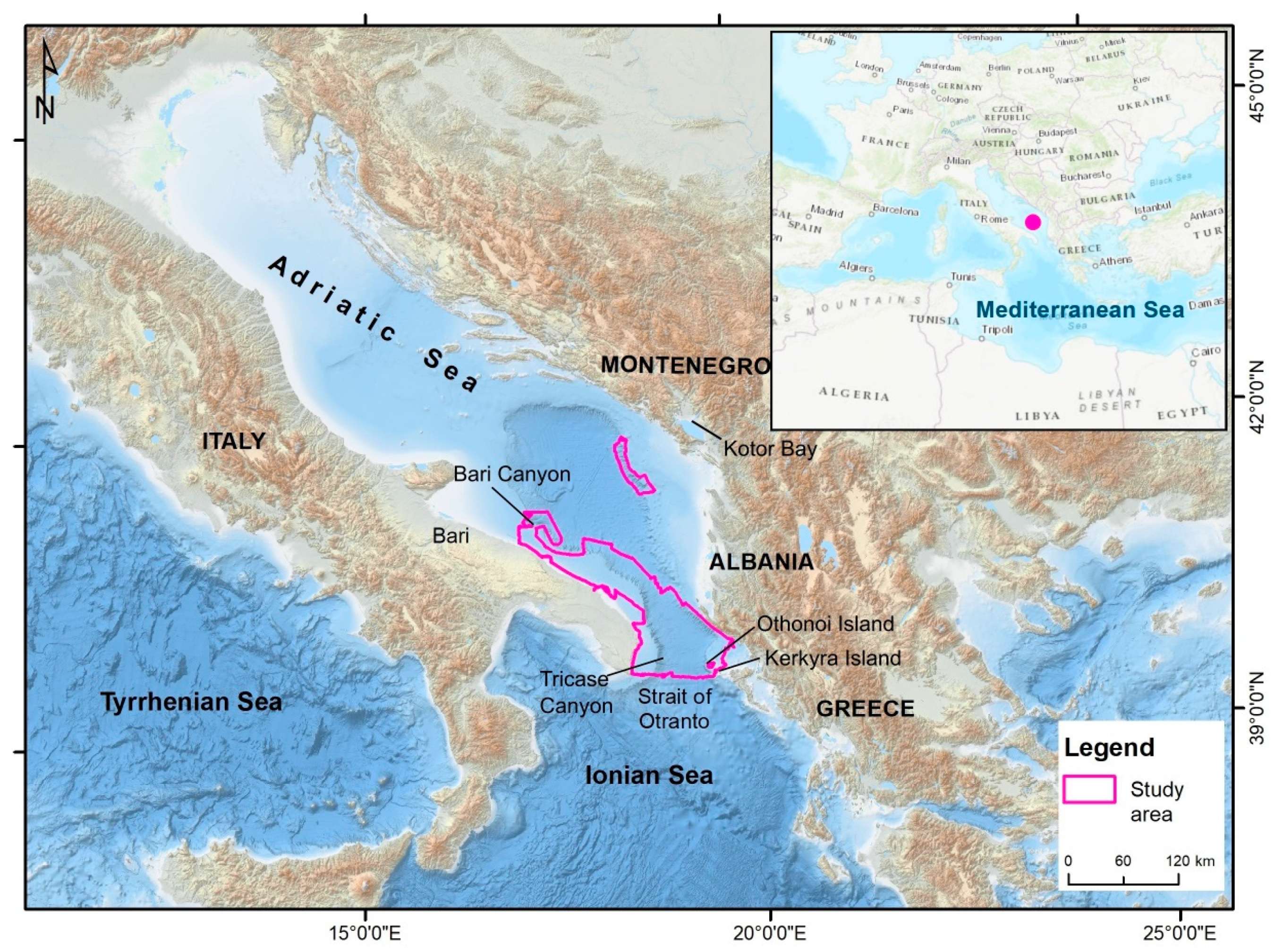
The area considered in this paper includes the Adriatic basin (continental shelf and slope) bordered northward between the Bari Canyon (Italy) and the Kotor Bay (Montenegro) and southward by the Strait of Otranto between Santa Maria di Leuca and Kerkyra Island (Figure 1).

Figure 1.
Location of the study area in the southern Adriatic Sea with a general view of the EMODnet bathymetry [42].
3. Materials and Methods
3.1. Datasets
The area has been surveyed repeatedly, resulting in the acquisition of ca. 13,400 km2 of high-resolution bathymetry and acoustic reflectivity data, while 255 seafloor samples were acquired by means of large volume grabs, box-corers, dredges and ROV surveys. In particular, acoustic reflectivity data constitute a patchwork of heterogeneous datasets acquired during 12 cruises carried out for a variety of purposes, using different devices and frequencies (Figure 2 and Table 1). Multibeam data have been processed using both PANGEA Multi Beam System and CARIS HIPS and SIPS, while the TOBI side scan sonar image was acquired and processed by means of PRISM software [8,11,12,43,44].
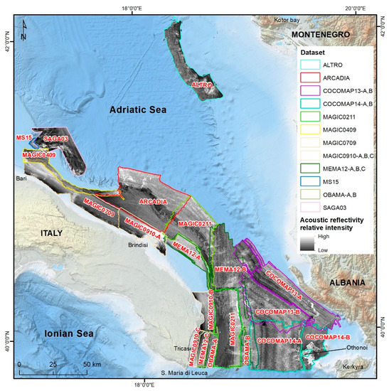
Figure 2.
Acoustic reflectivity mosaics acquired along the southern Adriatic Sea by ISMAR-CNR of Bologna (please refer to the Research Object http://www.rohub.org/rodetails/RSOBIA_Ad-1/overview for details, accessed on the 21 July 2021).

Table 1.
Technical specifications of the sonar devices used to acquire MBES and side scan sonar backscatter data.
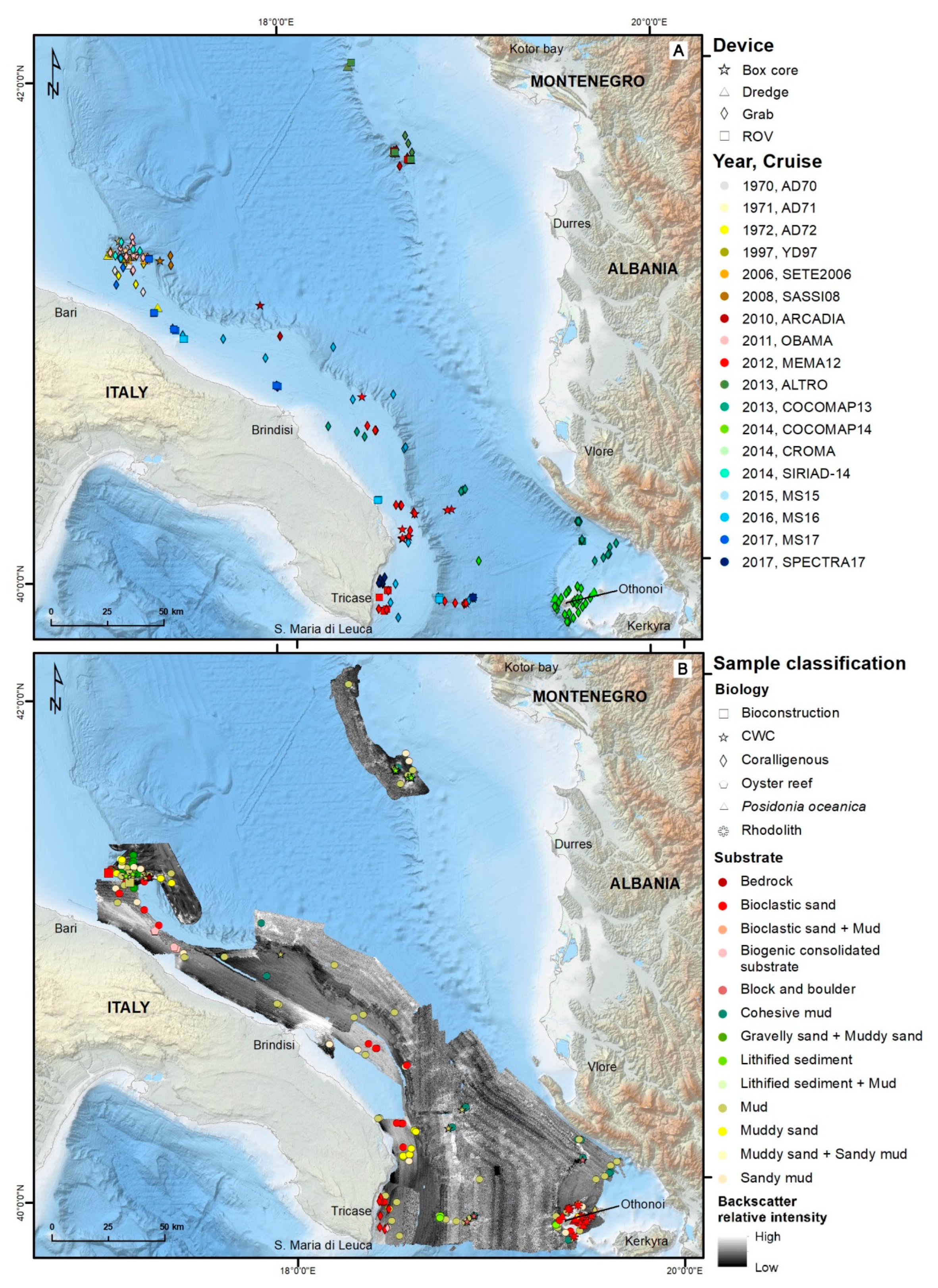
Ground-truthing is based upon 255 bottom samples collected during 18 cruises and stored in the CNR-ISMAR repository and geodatabase (Figure 3; for samples collected during the 1970s, we referred to [45]).

Figure 3.
Spatial distribution of the samples collected in the study area during the period 1970–2017. In (A) the samples are classified according to the gear used (symbols) and the cruise with year during which they were collected (colours). In (B) the samples are classified according to their substrate (colours) and biological description (symbols) using the classes proposed in the classification scheme applied in this work. Please refer to the Research Object http://sandbox.rohub.org/rodl/ROs/RSOBIA_Ad-1/ for details (accessed on the 21 July 2021).
3.2. Remote Sensing-OBIA (RSOBIA)
We performed an image analysis of backscatter, bathymetry and bathymetric derivatives based on the identification of objects (Object-Based Image Analysis, OBIA). The image is segmented into concrete natural objects [46,47] based on the shape of the clusters and their spatial correlation [5], and on the homogeneity within the clusters [48]. Among the different software enabling to perform OBIA (e.g., eCognition, GEOBIA), we chose to test the Remote Sensing-OBIA (RSOBIA) [25], a user-friendly toolset developed for ESRI ArcGIS 10.x that allows execution of an unsupervised segmentation on a single or multiple bands image.
In this work, every dataset was processed independently because (i) they were acquired during different surveys, (ii) with different devices and (iii) without following a standard process for the acquisition of calibrated backscatter. Hence, the backscatter images were not comparable to each other, and the datasets could not be merged or analysed together. Classifying the different multisource coverages separately allowed a relative comparison of backscatter.
The processing consisted of four main steps: (1) preparation of the input datasets (processing and extraction of MBES bathymetries and backscatters through CARIS HIPS and SIPS and calculation of bathymetric derivatives), (2) segmentation by means of RSOBIA, (3) classification through ground-truthing and expert opinion, and (4) validation. We formalized the part of the workflow implemented in ArcGIS using Model Builder for ArcGIS 10.5 (Figure 4). This tool makes the process from segmentation to ground-truthing automatically repeatable and reusable.
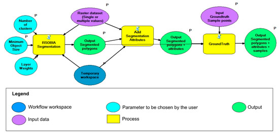
Figure 4.
Executable workflow built-in Model Builder (ArcGIS 10.5) and including the RSOBIA tools used in the present work (yellow), the input data — raster datasets to be segmented and ground-truthing data — (purple), the segmentation parameters to be chosen by the operator (light blue), the results (green) and the temporary workspace (dark blue). The workflow is available through the Research Object at the link: http://sandbox.rohub.org/rodl/ROs/RSOBIA_Ad-1/ (accessed on the 21 July 2021).
The input data for the segmentation were homogenized to a resolution of 10 m, they consisted of backscatter images from MBES and SSS, bathymetry, and the terrain attributes calculated through RSOBIA toolset (Slope, Roughness and Bathymetric Position Index—BPI). RSOBIA segmentation was run setting the Minimum Object Size at 1000 for all datasets: this value corresponds approximately to a circle of 18 pixels (180 m) radius which we found suitable for the scale at which we wanted to produce the benthic habitat map (basin scale: 1:300,000). The Number of Clusters changed for each dataset according to the substrate classes that we expected to find in every area, following the Calinski–Harabasz criterion [49]: higher is the ratio between the variance among and within clusters, better is the separation among the clusters.
We ran preliminary tests in order to identify the most efficient variables combination and their relative weights within the analysis, the best values for the Number of Clusters, and finally, the Minimum Object Size [25] to segment the images. We judged the adequacy of parameters in capturing the features of interest at the scale of work basing on visual interpretation. Following the methodology proposed by Lacharité et al. [23], we firstly included only the primary acoustic data layers (backscatter and bathymetry) to minimize the propagation of uncertainty during segmentation, assigning the backscatter twice the weight of bathymetry to give priority to the substrate composition, rather than local variability in depth and morphology. After a visual exploration of the acoustic data layers, we decided to include different terrain attributes (slope, BPI and roughness) tailored to the area being analysed in order to enhance morphological expressions, such as positive reliefs due to rock outcrops, erosive remnants, landslide blocks and any bioconstruction features (e.g., coralligenous formations and oyster reefs). In particular, we combined the acoustic backscatter data, bathymetry and slope for regular and smooth seafloor with low or no variation in roughness, such as large shelf sectors, large basin sectors or datasets including smooth shelf, slope and basin (as suggested by Lacharité et al. [23] and Innangi et al. [26]). When the seafloor was characterized by morphological variability, we combined backscatter with bathymetry, slope and roughness or BPI according to the kind of morphologies occurring on the area. We took into account the BPI calculated with a window size of 3 × 3 pixels for the areas showing positive reliefs or erosive remnants possibly made of bedrock or bioconstructions. We included the roughness into the segmentation when seafloor morphology was irregular, such as when occurring rhodolith beds (COCOMAP14-A) or coralligenous formations (MEMA12-C). In order to evaluate which combination of variables and weights was the best for each survey area, we also exploited the statistical measures (i.e., mean and standard deviation) associated with every polygon for each layer used for segmentation and calculated through RSOBIA toolset. This function allowed us to identify outliers among the isolated polygons.
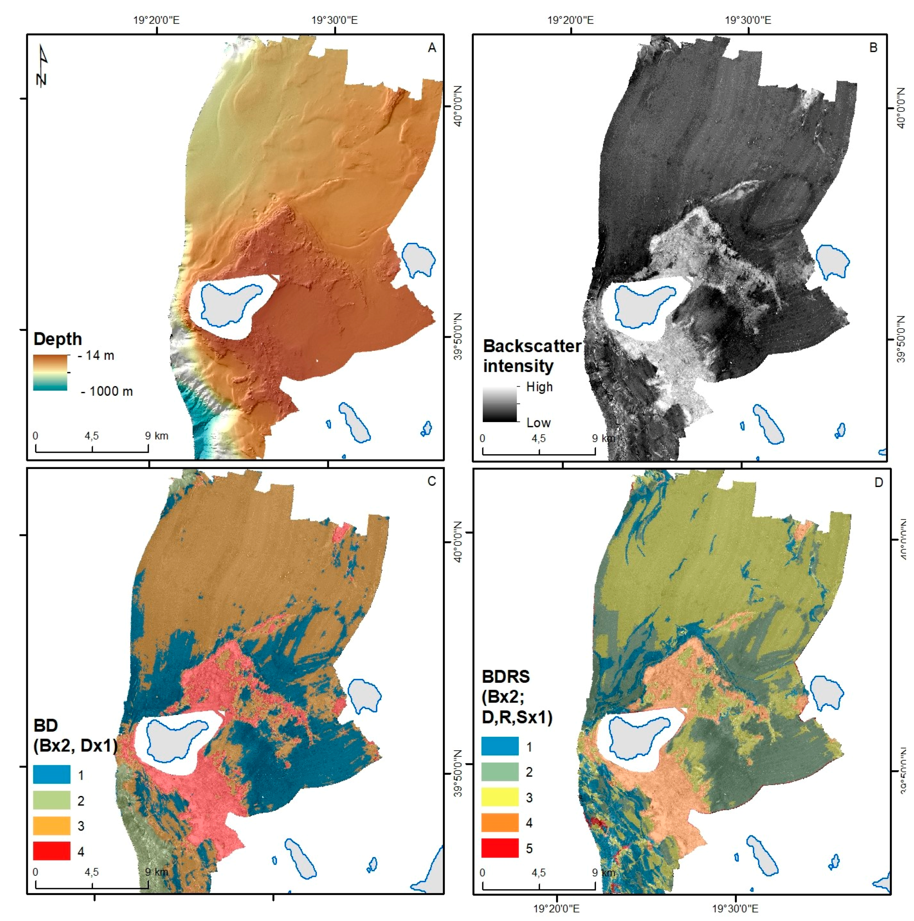
Figure 5 shows an example of RSOBIA segmentation run on COCOMAP14-A dataset using different variables. In the first case (Figure 5C), RSOBIA segmented a multi-layered image constituted by the backscatter and the depth, by giving the backscatter twice the weight of the bathymetry. The BD (Backscatter-Depth) datasets were segmented into four classes (Majority 1–4). In the second case (Figure 5D), the segmented multi-layered image included backscatter, depth, roughness and slope. The backscatter was analysed with a weight twice the other variables and we obtained five classes (Majority 1–5) from the segmentation of BDRS (Backscatter-Depth-Roughness-Slope) datasets.

Figure 5.
(A) Bathymetry and (B) Backscatter offshore Othonoi Island (Greece) acquired during COCOMAP14-A campaign using EM710 MBES; (C) Classes obtained through RSOBIA segmentation of Backscatter and Depth (BD) giving the backscatter twice the weight of the depth (B × 2,D × 1); (D) RSOBIA segmentation of Backscatter, Depth, Roughness and Slope (BDRS) giving the backscatter twice the weight of other variables (B × 2, D × 1, R × 1, S × 1).
Table 2 summarizes the variables and the parameters used in this work, showing heterogeneity between datasets. About variables, backscatter was given twice or thrice the weight of the other terrain attributes in all datasets, in order to ensure more importance to seabed reflectivity in the segmentation. For SAGA03, MS15, OBAMA and ALTRO datasets, we segmented only the SSS and MBES backscatter images because, through visual interpretation, we noted that acoustic reflectivity segmentation well isolated the most relevant features for the benthic habitats and that the inclusion on bathymetry and its derivatives did not give more information to improve the benthic habitat classification.
Table 2.
For each dataset, the table shows the input variables, their relative weights, the parameters (Number of clusters and Minimum Object Size) judged more efficient by the authors and then used in the segmentation, finally, the number of clusters resulting from RSOBIA segmentation.
In some cases, we set the Number of Clusters equal to 0 because this setting allows us to maximise the calculation based on the Calinski–Harabasz criterion, making the segmentation run for the best number of clusters [25]. In SAGA03, we decided not to limit the RSOBIA segmentation to a number of clusters exploiting side scan sonar image at its maximum. In COCOMAP14-A, we did not know which number of substrate classes to expect due to a high heterogeneity of substrates (witnessed by bottom samples) and acoustic facies. For the dataset ALTRO, we also did not know the expected number of classes given the limited number of samples ground-truthing the dataset and all concentrated in a small area. In addition, few works are available in the literature to gather more information on benthic habitats of the area.
The results of RSOBIA segmentation are polygonal shapefiles (one for each survey area) with the following attributes (definitions taken from [25]):
- ID: Consecutive number of polygon (useful for identification);
- AREA: Size of polygon (in units of the original imagery);
- MEAN: Average of classes of all pixels in polygon (useful for finding outliers);
- STD: Standard deviation of classes of all pixels in polygon (low values show good cluster correspondence);
- SUM: Sum of all classes of all pixels in polygon;
- MAJORITY: Most common class of all pixels in polygon (this is the main class for interpretation).
3.3. Classification
After obtaining a segmentation of all the datasets with RSOBIA, we converted the classes into benthic habitats by comparison with ground-truthing and the literature data. We applied the function “Groundtruth Samples” of RSOBIA tool to associate the information related to bottom samples and images to the classes (i.e., Majority values) identified by RSOBIA during the segmentation. Majority values were correlated with sample description and used to infer the benthic habitat types. When surveys were poorly sampled or not sampled at all, we exploited the literature data in order to infer the benthic habitats characterizing them. In particular, we exploited the works [36,50,51,52,53] to gather information on coralligenous formations and oyster reefs, [12,16,17,18,54,55,56,57] to collect details on Bari Canyon cold water corals (CWCs) and [16,58] to assemble data on CWC communities of Gondola slide and offshore Monopoli, respectively. Finally, when either ground-truthing or literature data were not available or classes hosted multiple samples of different lithologies, we inferred the benthic habitats occurring there through expert interpretation [27].
After naming the classes of all the segmentations, we merged all the shapefiles into a single one reporting the classification of the benthic habitats of the southern Adriatic basin.
Noise and holes in datasets were automatically identified in the images by RSOBIA that created a class including these artefacts (mainly located at the nadir or overlapping areas) and no-data areas (often the class named Majority 0 includes these “anomalies”). Hence, we were able to delete areas with no data (i.e., holes) or merge areas presenting noise with the adjacent, case-by-case.
We fixed no-data areas (i.e., holes) using the “Topology toolbar” of ArcGIS software and merged the classes related to noise with the adjacent ones.
Finally, we used the “Simplify polygon” tool (BEND_SIMPLIFY algorithm with a tolerance of 100 m) of ArcGIS software to simplify polygon features by removing relatively extraneous vertices and preserve essential shape to obtain a better cartographic result.
We built the legend following a hierarchical classification scheme, developed in-house specifically for the Mediterranean and Black Seas, conceived in the framework of the European Project CoCoNet [58] and still under review, but already successfully applied in benthic habitat mapping ([12,13,18] and references therein).
3.4. Validation
To test the accuracy of our classification, we compared our prediction with bottom samples. An amount of 70% of samples (178 of 255) were randomly selected and used to name the classes, while the remaining 30% (77 of 255) were used for testing prediction reliability. The overall accuracy, which represents the percentage of cases correctly allocated, was calculated by dividing the total number of correct allocations by the total number of samples. Class-specific accuracy was also calculated for each reference and predicted class. The first corresponds to how well reference samples are classified, while the second represents the probability that a pixel classified into a given category represents that category on the ground. The analysis was performed in R software [59] using “confusionMatrix” function of the “caret” package [60].
4. Results
4.1. RSOBIA Segmentation Results
The segmentation results for the entire study area are shown in Figure 6, Figure 7, Figure 8 and Figure 9 and described below.
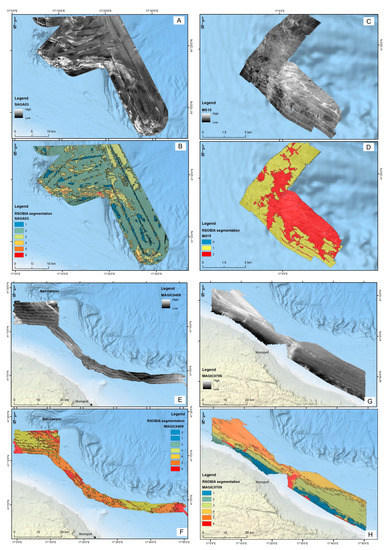
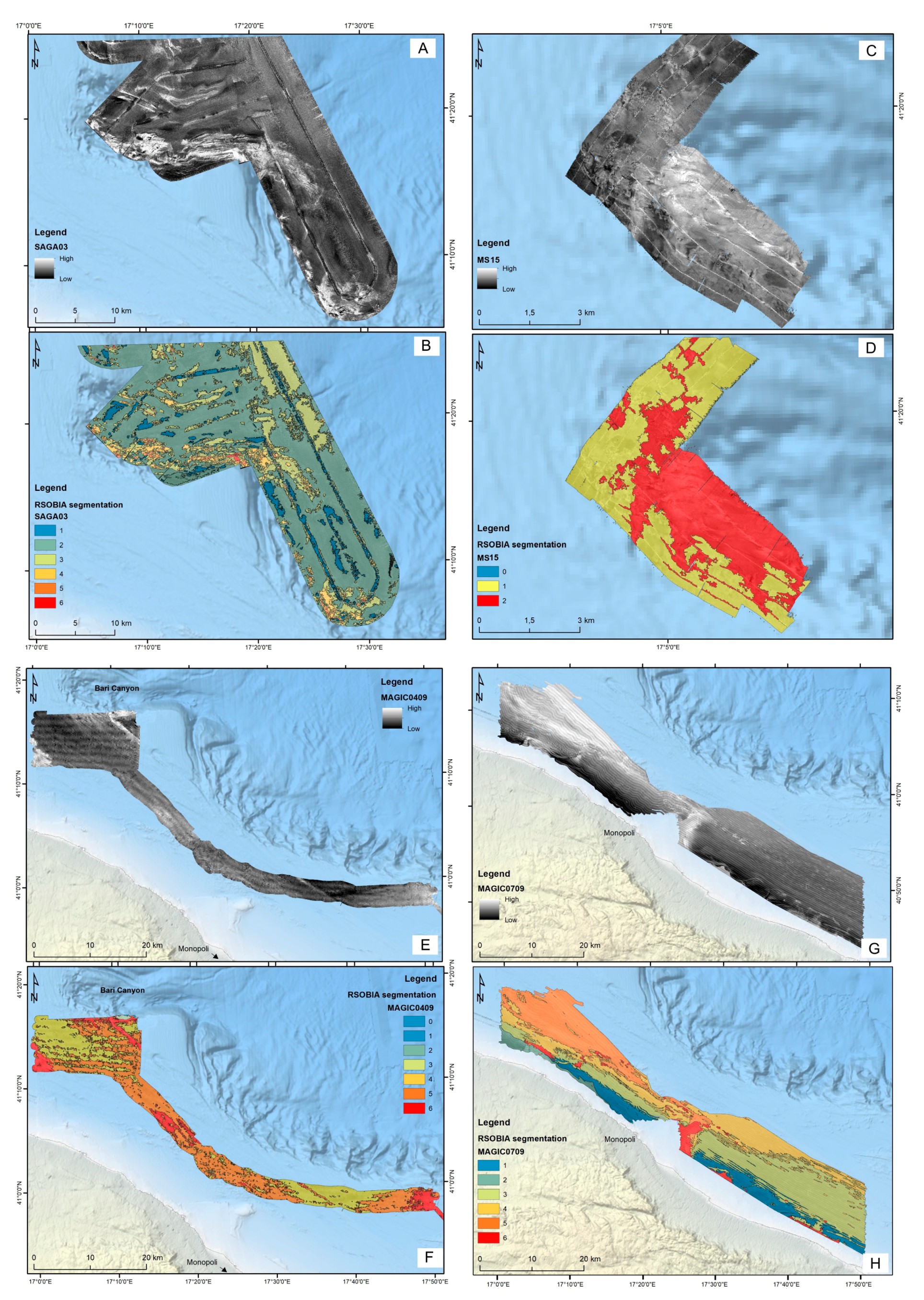
Figure 6.
Backscatter images and results of RSOBIA segmentations for the datasets SAGA03 (A,B), MS15 (C,D), MAGIC0409 (E,F) and MAGIC0709 (G,H).
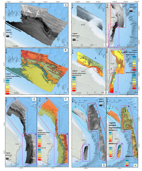
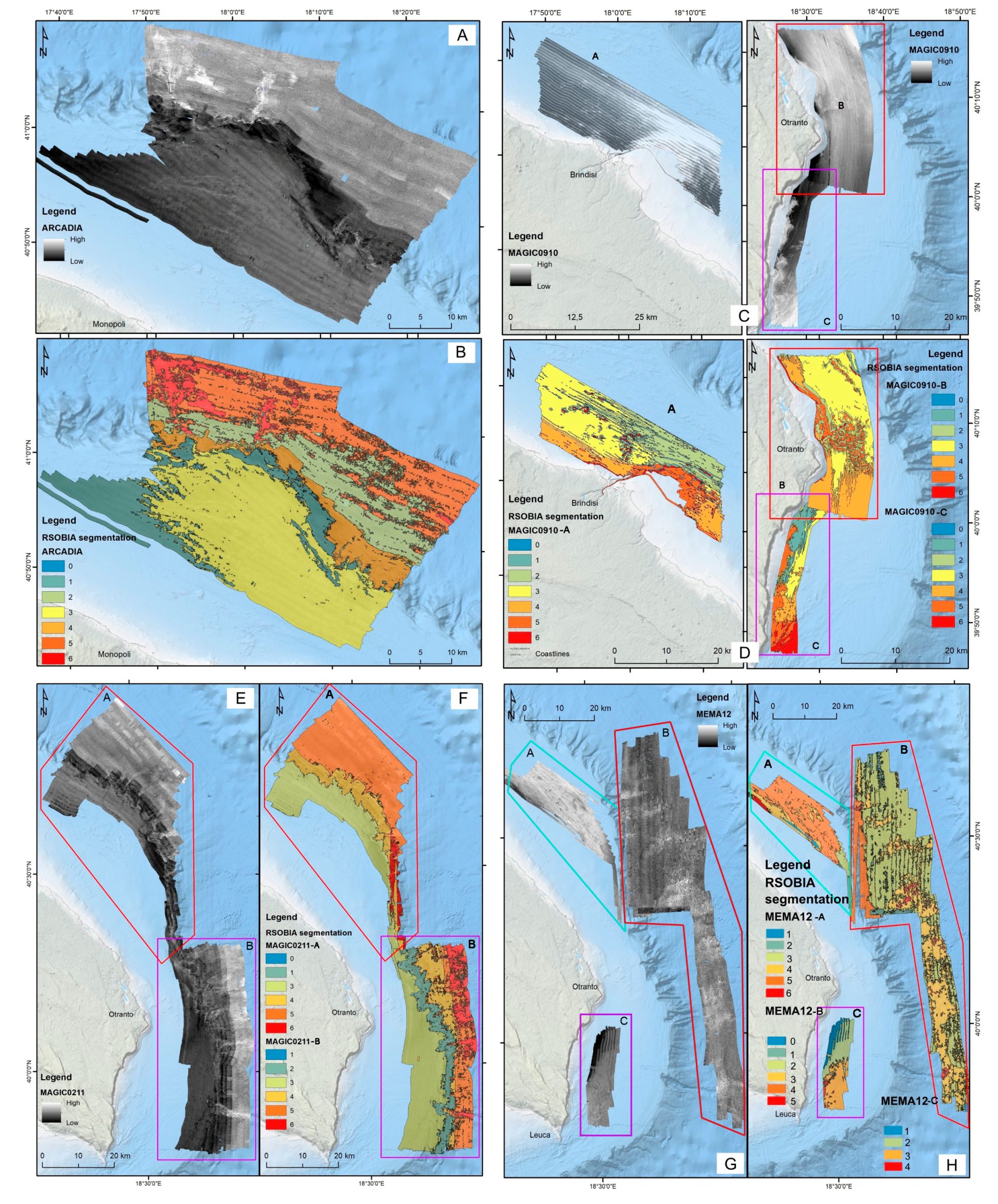
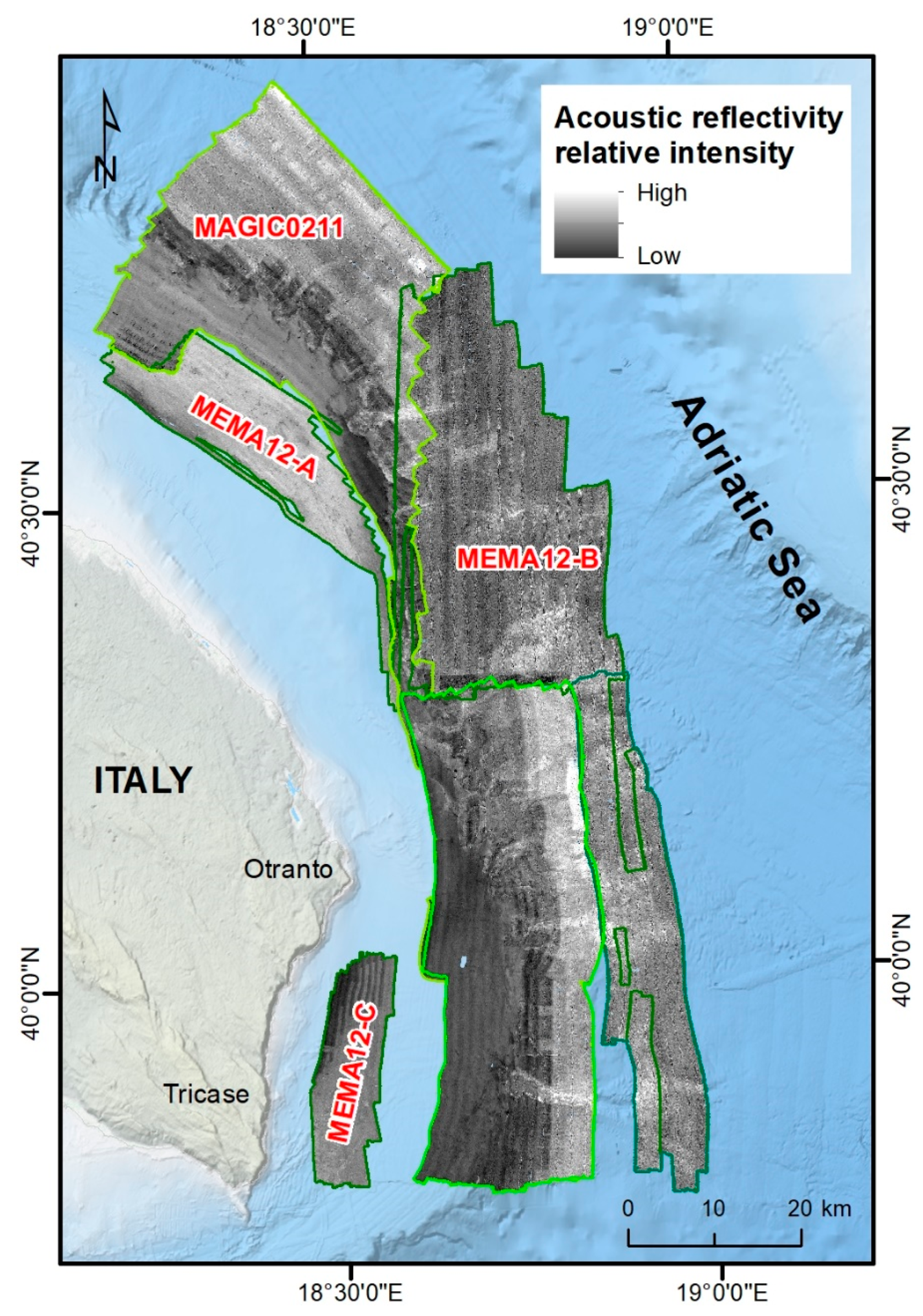
Figure 7.
Backscatter images and results of RSOBIA segmentations for the datasets ARCADIA (A,B), MAGIC0910 (C,D), MAGIC0211 (E,F) and MEMA12 (G,H).

Figure 8.
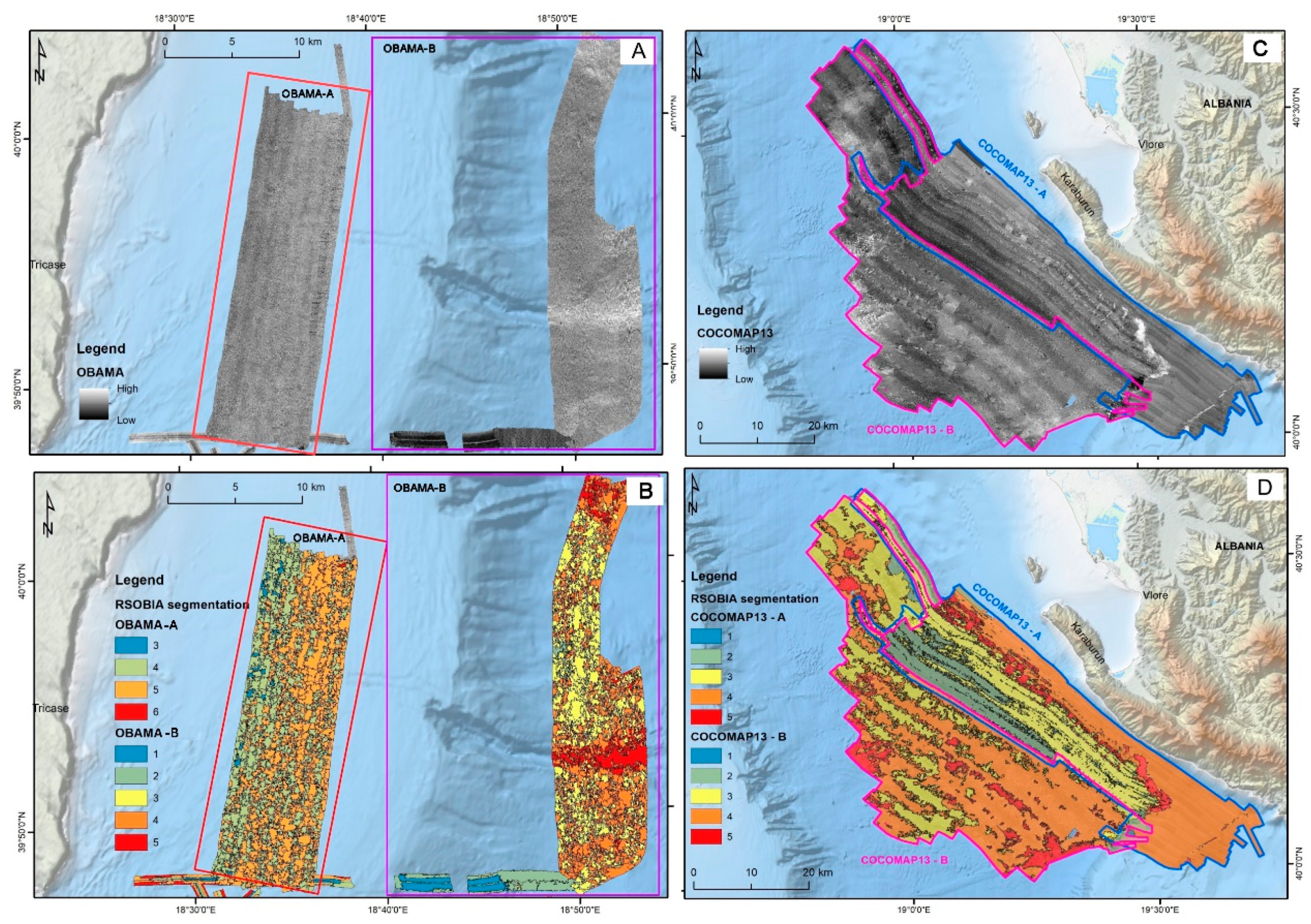
Backscatter images and results of RSOBIA segmentations for the datasets OBAMA (A,B) and COCOMAP13 (C,D).
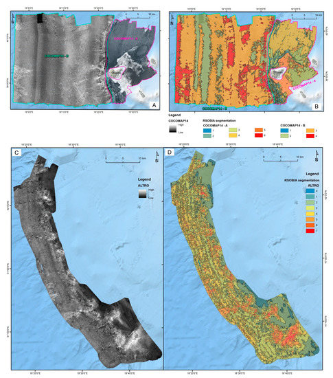
Figure 9.
Backscatter image and RSOBIA segmentation for the datasets COCOMAP14-A and -B (A,B) and ALTRO (C,D).
The segmentation of SAGA03 side scan sonar image (Figure 6A,B) resulted in six classes (Majority 1–6), where Majority 1 isolated noise at nadir. Majority 4–6 identified consolidated substrate areas hosting CWCs, while Majority 3 was interpreted as semi-consolidated substrate and Majority 2 as unconsolidated substrate. MS15 segmentation (Figure 6C,D) identified three classes (Majority 0–2), where Majority 0 isolated holes in the dataset. Majority 1 identified an area characterized by unconsolidated substrate, while Majority 2 isolated an area of high backscatter corresponding to consolidated substrate. The segmentations of SAGA03 and MS15 acoustic reflectivity images showed a good match and continuity among classes with similar characteristics and statistics. Hence, also the classification through bottom samples resulted in consistency between these two areas.
The segmentation of MAGIC0409 (Figure 6E,F) matched well with the southern boundary of SAGA03 segmentation in isolating areas of coarse sediments (Majority 6) from the rest of the shelf characterized by fine sediments (Majority 3–5). Majority 0–2 isolated holes and boundaries in the datasets and small areas interpreted as mud. MAGIC0709 datasets (Figure 6G,H) showed a noisy backscatter image. There, the inclusion of bathymetry and BPI into the segmentation allowed us to isolate positive reliefs, successively interpreted as Oyster reefs, and to distinguish among coarse (Majority 4 and 5) and fine sediments (Majority 1–3).
In ARCADIA datasets (Figure 7A,B), RSOBIA segmentation resulted in seven classes (Majority 0-6), where Majority 0 identified small errors in the backscatter image. RSOBIA isolated the central and eastern area of the continental shelf (Majority 3) characterized by coarse sediments, from the muddy western area (Majority 1). Majority 4 isolated the shelf break constituted by lithified sediment, while Majority 2 and 5 were classified as muddy seafloor with small areas constituted by more consolidated substrate (Majority 6). In the MAGIC0910 datasets (Figure 7C,D), the segmentation identified positive reliefs, interpreted as Oyster reefs (Majority 6), and consolidated substrates, most likely made of coralligenous formations (Majority 5 in MAGIC0910-A and Majority 5 in MAGIC0910-C). The area of MAGIC0910-B is characterized by sediment waves that were isolated by including the bathymetry and slope into the analysis (Majority 2 and 5).
The segmentation of MAGIC0211 datasets (Figure 7E,F) identified: the continental shelf of muddy sand/sandy mud with Majority 3 in MAGIC0211-A and Majority 3 in MAGIC 0211-B; the shelf break made of lithified sediment with Majority 4 in MAGIC0211-A and Majority 1 in MAGIC0211-B; and, the slope and basin dominated by mud with Majority 5 in MAGIC0211-A and Majority 4 in MAGIC0211-B, except for the Tricase Canyon hosting consolidated substrates (blocks and boulders; Majority 5 and 6 in MAGIC0211-B).
The segmentation of MEMA12 datasets (Figure 7G,H) produced classes on the shelf highlighting the presence of small positive reliefs characterized by high reflectivity, successively interpreted as bioconstructions (Majority 5 in MEMA12-A) and as coralligenous formations (Majority 4 in MEMA12-C). In MEMA12-B, the segmentation highlighted the presence of two classes with positive reliefs characterized by high backscatter (Majority 4 and 6), then interpreted as cohesive mud or rock blocks potentially hosting CWCs. These classes are surrounded by slope and basin floor made of mud (Majority 5 and 3, respectively). Majority 1 and 2 in MEMA12-A identified noise in backscatter image.
OBAMA datasets (Figure 8A,B) were very noisy and RSOBIA failed in finding objects in OBAMA-A that was segmented into four classes not supported by ground-truthing. On the contrary, in OBAMA-B, RSOBIA succeeded in isolating patterns that were then interpreted as cohesive mud and rock blocks hosting CWCs (Majority 4 and 5). COCOMAP13 datasets (Figure 8C,D) are characterized by backscatter images containing noise and errors among adjacent lines that are visible in the segmentation. However, patterns located at the shelf break and in the basin floor (Majority 5 in both the datasets), interpreted as cohesive mud and consolidated substrate hosting CWCs, were isolated by including bathymetry and slope into the analysis. The rest of the datasets was classified into a single benthic habitat class, as witnessed by ground-truthing.
The segmentation of COCOMAP14-A (Figure 9A,B) resulted in a large number of classes (Majority 1–6), in line with the high variability in seafloor morphologies, substrates and habitats. This segmentation was detailed especially in shallow water areas hosting rhodolith beds and in few areas located north. The backscatter of COCOMAP14-B is noisy, and errors among adjacent lines are also highlighted in the segmentation. However, the inclusion of bathymetry and slope into the analysis helped us to isolate the more consolidated substrate (Majority 4). Majorities 1–3 were classified into a single benthic habitat class, as witnessed by ground-truthing. The segmentation of ALTRO backscatter image (Figure 9C,D) was noisy and with a high number of classes (Majority 0–7, where Majority 0 isolates holes in the datasets). Such a large number of classes allowed us to clearly identify features characterizing the slope and hosting CWCs and coral forest surrounded by a muddy seafloor.
4.2. The Benthic Habitat Map of the Southern Adriatic Sea
The main result of this work is the “Benthic habitat map of southern Adriatic Sea (Mediterranean Sea)” (scale 1:300,000), showing 13 types of substrates and 8 benthic habitats, here illustrated in a simplified view in Figure 10 and with more details in Supplementary, Figure S1. The full description of codes reported in the legend of Figure 10 is shown in Table 3.
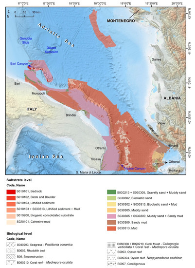
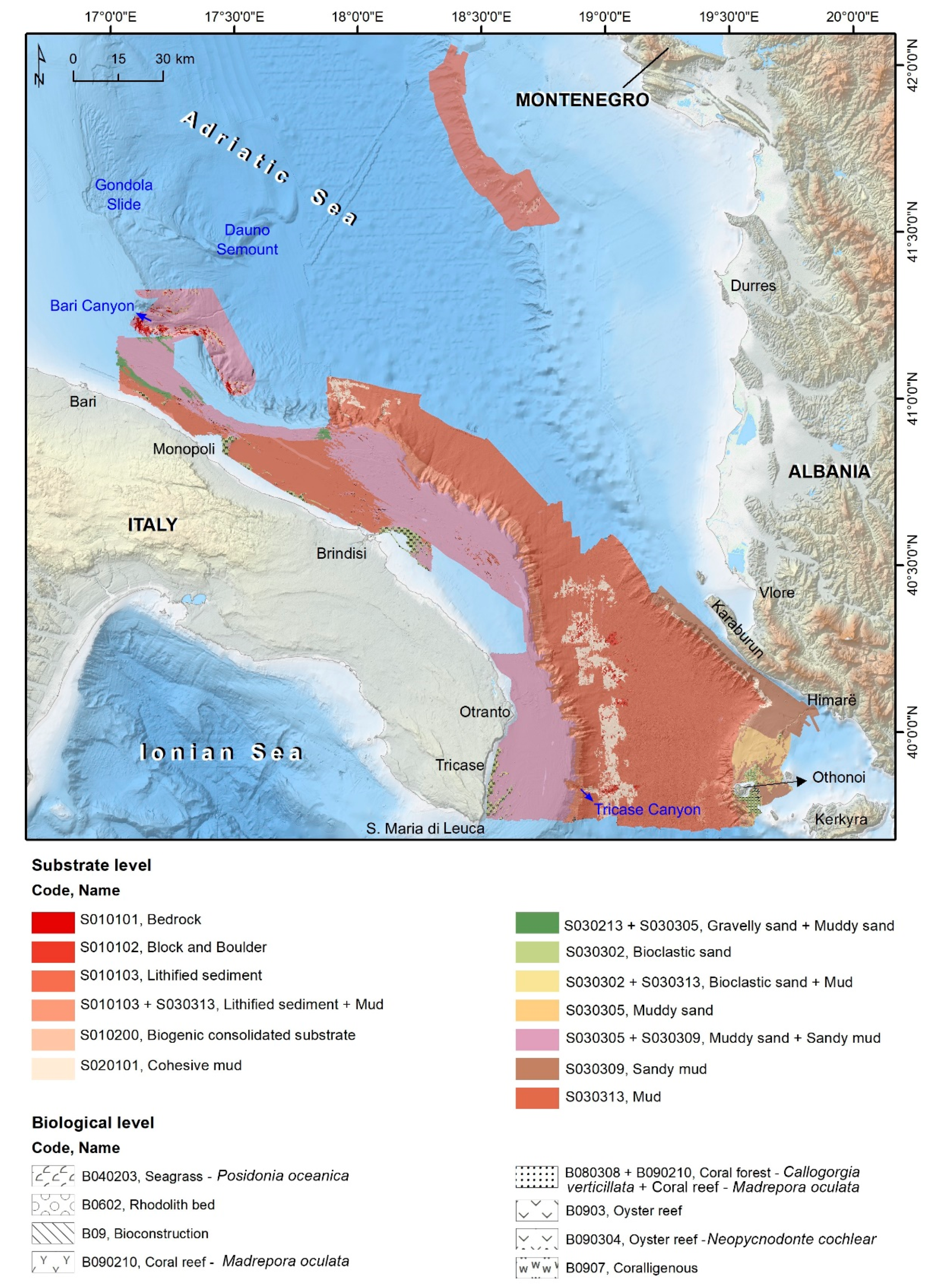
Figure 10.
Benthic habitat classification of the southern Adriatic Sea resulting from RSOBIA segmentation, ground-truthing through samples and images of the seafloor, expert interpretation and comparison with published data. For a more detailed version of the map, please refer to the “Benthic habitat map of the southern Adriatic Sea (Mediterranean Sea)” provided as supplemental material (Supplementary, Figure S1). Results are also available in digital versions through the Research Object: http://sandbox.rohub.org/rodl/ROs/RSOBIA_Ad-1/ (accessed on the 21 July 2021). The full description of codes reported in the legend is shown in Table 3. Some classes of the legend were created by combining two codes: for example, the class “S010103 + S030313, Lithified sediment + Mud” is obtained coupling “S010103, Lithified sediment” with “S030313, Mud”.
Table 3.
Complete description of the codes used in the legend of the benthic habitat map (Figure 10). Both substrate and biological components are subdivided into three levels, going from general/large scale to detailed/small scale features.
4.2.1. Western Side
Most of the western continental shelf is covered by fine sediments, primarily muddy sand and sandy mud. The Apulian shelf hosts at depths shallower than 100 m, bioconstructions (i.e., coralligenous formations) and oyster reefs dominated by the gryphaeid Neopycnodonte cochlear, e.g., [36,50,51,52,53].
Moving south, the shelf is still dominated by muddy sand and sandy mud, alternated, often associated with coralligenous formations (Fine unconsolidated substrate--Bioclastic sand + Bioconstruction-Coralligenous), as mapped also during BIOMAP Project [50,61]. The sediments characterizing western shelf and slope seem to be linked to the sediment supply from the Italian mainland thanks to the contribution from fluvial input, such as Po River and Apennines’ rivers ([62] and references therein).
The Apulian continental slope is affected by mass failures [8,11] resulting in the accumulation of blocks [63] onto the basin floor mapped as cohesive mud, and blocks and boulders hosting CWCs. This margin is also affected by multiple incisions whose heads, in correspondence with the shelf break, appear to be made of lithified sediment [64]. The two main incisions are Bari and Tricase canyons, hosting healthy and lush CWC ecosystems [13,16,54,56,57,58,59,60,61,62,63,64,65]. Their upper slope is made up of bedrock, lithified sediment or firm ground (i.e., semi-consolidated) in correspondence of shelf break, canyon heads or landslide scars, being suitable for CWCs settlement, e.g., [12,17,18,54,55,56]. The channels of the above-mentioned incisions are characterized by mixed and/or compacted sandy or muddy sediments that change into lithified sediments, in correspondence with the mass transport deposits that also include rocky blocks (seen isolated on the backscatter images) often hosting CWCs (as seen in the toe of the Tricase Canyon) [13,56]. This changes the interpretation to consolidated substrates occurring in the northern part of the canyon and along the SE slope for the following reasons:
- the areas containing samples proving CWC occurrence have been interpreted as consolidated substrates;
- CWCs presence was reported also in sites located at ca. 45 km north and northeast of Bari Canyon (Gondola Slide and Dauno Seamount) [16], and ca. 55 km southward in the deeply incised slope offshore Monopoli [57].
4.2.2. Eastern Side
The Montenegrin and Albanian (Karaburun Peninsula) shelf is flat, narrow, NW-SE oriented and covered by fine sediment, mainly mud. Near the shelf break, patches of cohesive mud are probably due to the presence of erosive remnants. Offshore Himarë (Albania), the continental shelf varies orientation to N-S due to a change in the tectonic setting [28]. South, the Othonoi shelf is characterized by a rock outcrop extending about 5 km north and south the island. The change in tectonic setting is observable as a transition from a muddy seafloor with areas of cohesive mud and lithified sediment (Montenegrin and Albanian shelf) to a karst landscape [66] surrounded by a sandy and gravelly seafloor, and hosting rhodolith facies and Posidonia oceanica meadows around Othonoi Island (cf. inset of Rhodolith beds and seagrass meadows offshore Othonoi Island shown in Supplementary Figure S1). Indeed, the variation in tectonics is also responsible for the different sediment supply from the land, hence influencing the material reaching the seafloor.
The eastern continental slope is affected by mass wasting processes that favoured the development of a large number of incisions [37,38,39] made of muddy sedimentation with lithified sediments and hardground in correspondence of few areas of the shelf break. In particular, the Montenegrin slope is characterized by consolidated substrates in correspondence of shelf break and scars. An area of lithified sediment of about 10 km2 located at a water depth of 430–490 m on the slope of a slump scar is most likely due to the presence of a carbonate chimney forest [67]. This area constituted by hard substrates hosts coral forests, mainly typified by Callogorgia verticllata [56,68] and CWCs best embodied by Madrepora oculata and Desmophyllum pertusum, [56,67].
4.3. Accuracy Assessment
The overall accuracy of RSOBIA classification was equal to 45% (Table 4). Although low, this value is in line with accuracies calculated in previous studies using this methodology [12]. The analysis of class-specific accuracies provides a more complete vision, showing some classes presenting high accuracies (up to 100% of corrected classified samples) while other reporting very low values (Table 4). This might be related to the higher similarity in terms of terrain variables among some classes that differed for substrate typology (e.g., sands, mud) potentially resulting in a less precise definition of borders. Moreover, seafloor heterogeneity at small-scale is not properly represented in the classification of such a large area, unavoidably influencing model accuracy. The presence of biological features with distinguishable reflectivity and terrain characteristics (e.g., Rhodolith beds, P. oceanica meadows, corals) appeared to facilitate the segmentation, providing higher accuracies in some situations.
Table 4.
Confusion matrix assessing the accuracy of the final substrate and benthic habitat classification of the southern Adriatic Sea. The codes refer to the following benthic habitats: S010101, Bedrock; B090210, Coral reef-M. oculata; S030302, Bioclastic sand; S030302 + B0602, Bioclastic sand + Rhodolith bed; S030302 + B09, Bioclastic sand + Bioconstruction; S030302 + B0907, Bioclastic sand + Coralligenous; S030302 + B040203, Bioclastic sand + Seagrass-P. oceanica; S030302 + S030313 + B0907, Bioclastic sand + Mud + Coralligenous; S0102+B09, Biogenic consolidated substrate + Bioconstruction; S010102 + B090210, Block and boulder + Coral reef-M. oculata; S0201, Firmground; S0201 + B090210, Firmground + Coral reef-M. oculata; S030213 + S030305, Gravelly sand + Muddy sand; S010104, Lithified sediment; S010104 + B090210, Lithified sediment + Coral reef-M. oculata; S010104 + S030313 + B090210, Lithified sediment + Mud + Coral reef-M. oculata; S030313, Mud; S030313 + B090210, Mud + Coral reef-M. oculata; S030305, Muddy sand; S030305 + S030309, Muddy sand + Sandy mud; S030309, Sandy mud.
5. Discussion
Benthic habitat maps are a simplified representation of actual seafloor and delineate perimeters around areas with similar properties (e.g., physical characteristics or biological communities) [27]. The use of different combinations of acoustic layers and terrain attributes has been proved to be effective in isolating and characterizing specific habitats or features; for example, coral mounds [69], habitats settled on positive reliefs breaking the continuity of a planar seafloor [7] or large-scale habitats, such as canyons [70]. For this reason, we proceeded in segmenting and classifying each dataset separately, combining backscatter, bathymetry and terrain attributes (different combinations for each dataset). Then, we integrated the separated classifications in a single final classification, producing a single and consistent benthic habitat map for the southern Adriatic basin.
During this challenging work, we faced issues related to underwater acoustics, classification and ground-truthing.
5.1. Acoustic Issues
The use of uncalibrated and non-comparable mosaics of backscatter and side scan sonar is the main obstacle that causes incoherence in the classifications among dataset boundaries. A possible solution is the estimation of the dataset-to-dataset offsets and then the association of these values as bulk shifts in the absolute scattering strength estimates [71]. However, slight disparities among backscatter mosaics would persist, because there are other factors accounting for these shifts, such as imperfect attenuation coefficients (e.g., sea water attenuation coefficient dependent on water temperature and salinity) and frequency dependence of scattering, which controls acoustic signal penetration in sediments [72,73].
In our study, discrepancies are visible also within a same dataset, acquired with the same device, within the same cruise and same version of acquisition software, for example MAGIC0211 and MEMA12. There, a change in depth (from shelf to slope and basin floor) brought the device to change setting automatically (pulse length, frequency and power, as well as attenuation), causing a change in backscatter strength among adjacent lines (Figure 11). These issues affected the segmentation of the datasets creating different classes for the same type of substrate as demonstrated by the groud-truthing (e.g., Majority 4 and 5 of MAGIC0211-B in Figure 7). Since we were not able to calculate bulk shifts among the acoustic reflectivity images, as suggested above, we faced these issues during the classification step: we merged the classes that represented the same type of substrate following ground-truthing data, the literature data and our interpretation.

Figure 11.
Area of junction between the two datasets MAGIC0211 and MEMA12, both of them acquired with Kongsberg EM710 and characterized by changes in backscatter intensity, line by line and within the same dataset.
Seabed acoustic backscatter is constituted by surface scattering—generated by the interaction of the acoustic wave with the seafloor surface—and volume scattering, produced by its interaction with a sediment volume [74]. Generally, the acoustic signal penetrates deeper in unconsolidated sediments (i.e., mud) than in consolidated substrates (e.g., rocks) and constitutes a high contribution in backscatter signal when using low frequency’s sonar systems. The interaction signal-sediment volume occurs more often when the sediment contains ‘discontinuities’ (e.g., gas bubbles, benthic organisms, shell fragments, or sediment particles themselves) that cause slight changes in sound speed or density [3,12,74]. This fact results in incongruities between the backscatter response and the sediment sampled from the seafloor. For example, in our study, breaks of slope, ridges or other features characterized by steep slope and/or positive relief covered by a thin layer of fine sediment show a high response in backscatter. This can be induced both by the influence of seabed morphology and/or incident angle on backscatter data, and by the penetration of acoustic signal into the thin and soft layer of unconsolidated sediment. Even if backscatter is processed using the Geocoder algorithm corrected for the depth using the “adaptive” mode, for high incident angles it happens that the morphological effects are not totally eliminated. This is the case of the heads of the Bari and Tricase canyons and the Albanian continental margin scars and incisions: there, bottom images demonstrate that the bedrock is constituted by rocky substrate partially covered (often less than 5–10 cm) by mud, e.g., [12,13,16,18,57]. In these cases, the backscatter signal (frequency of 70–100 kHz) constitutes a predominant response to the underlying hard substrate more than to the easily penetrable, thin, fine sediment drape.
When we encountered this kind of incongruity, we chose the type of substrate more significant in terms of benthic habitats eventually hosted or we combined more classes in order to keep as much information as possible (e.g., “S010103 + S030313, Lithified sediment + Mud”). In the cases of Bari and Tricase canyons, we classified ambiguous areas as consolidated substrate because the presence of bedrock or lithified sediment (= loose grain sediments under process of rock formation, such as fluid expulsion and compaction), even if draped by fine sediments, would favour the settlement of megabenthic organisms, such as corals.
One of the consequences of the frequency-dependence of backscatter signal is its dependency on wavelength. Hughes Clarke et al. [72] reported the example of an area surveyed with two different devices with different frequencies. It resulted that backscatter intensity was almost the same in higher backscatter areas, while soft sediment areas showed greater variability. This is because the grain size of harder/coarser substrates has a wavelength much larger than both devices’ wavelength, while fine-grained sediments have a wavelength comparable to higher frequency device wavelength. Hence, since the acoustic response of the seafloor is wavelength dependent, classifications might proceed quite differently depending on the wavelength used. This results in a good match among different backscatter datasets for what concerns high backscatter values corresponding to hard substrates (such as for SSS backscatter of SAGA03 and MBES backscatter of MAGIC0409 and MS15 shown in Figure 12B) that are easily detected by any segmentation and classification methods. On the contrary, areas of intermediate values of acoustic reflectivity, corresponding to unconsolidated substrates, show higher variability in the acoustic mosaics as well as in segmentation and classification results.
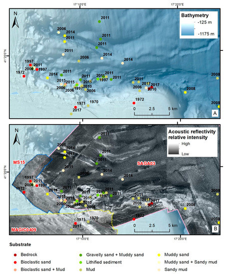
Figure 12.
Spatial and temporal distribution of bottom samples collected in the Bari Canyon since the 70s and classified according to their description, showing a consistency in types of substrates sampled through time; (A) shows the morphology of the Bari Canyon and (B) shows the acoustic reflectivity images collected there and their good match in correspondence of high reflectivity areas.
5.2. Ground-Truthing Issues
Cruise sample strategies were not always appropriate for seafloor mapping, backscatter calibration or automatic backscatter segmentation and classification because samples were not collected in order to ground-truth the acoustic facies. There is a high concentration of samples in specific areas (such as Bari Canyon for their CWC ecosystems and Othonoi Island for the Rhodolith beds), while most of the continental shelf, slope and basin floor are undersampled. We solved this issue by inferring the benthic habitat classes through comparison with other available data (e.g., adjacent datasets, acoustic facies and classifications that had corresponding ground-truthing data andliterature data). Furthermore, the hierarchical classification scheme applied in this work allowed us to get a continuous and homogeneous cartographic product for the entire basin. This approach permitted us to map substrate and biology separately, allowing us to classify also areas where no biological information was available.
Another possible source of error is the temporal interval among the datasets and the temporal mismatch occurring also among the collection of samples and acoustic data. We assumed that no change has occurred in these years for what concerns main features, substrate and habitat occurrence. Changes might have occurred at a local scale (e.g., slight variations in grain size), but principal characteristics are maintained. An example of positive correspondence among bottom samples collected within an important span of time is notable on the Bari Canyon (Figure 12): there is no difference among bottom samples collected in the 70s and the most recent ones (2017). In case changes have occurred through time, then they were at a scale non-mappable for our work.
6. Conclusions
The aim of this work was to produce a benthic habitat map of the southern Adriatic Sea by combining all the acoustic reflectivity, bathymetry, bathymetric derivatives, ground-truthing and the literature data available for this basin. We analysed uncalibrated, non-comparable and non-overlapping seabed acoustic reflectivity datasets acquired during 12 cruises by means of five different devices. We used a semi-automatic approach consisting of an object-based image analysis of the acoustic data by means of the ArcGIS toolset RSOBIA [10] and the classification into benthic habitat classes. The result of this challenging work is the first and continuous benthic habitat map of the southern Adriatic Sea (from the Bari Canyon to Santa Maria di Leuca and including Montenegrin, Albanian and Greek margins) at 1:300,000 scale including information on both substrate and biology. This map will be a reference for future studies on substrate and habitat distribution changes occurring in the investigated area through repeated surveys and could be exploited as a basis for maritime spatial planning.
The great strength of this work is that we successfully applied a semi-automatic method on an inhomogeneous and large dataset (20 acoustic datasets collected within 12 cruises and 255 bottom samples collected during 19 cruises) never attempted before.
Most of the challenges encountered came from:
- Issues in segmenting and classifying acoustic facies, especially due to the use of uncalibrated and non-comparable acoustic reflectivity data (different SSS and MBES backscatter datasets, acquired with different devices, frequencies and oceanographic conditions);
- Sampling strategies carried out for different aims, not ground-truthing acoustic facies, and resulting in a dataset (i) with a sampling density highly variable within the mapped area and (ii) collected in a time span of about 50 years.
We overcome these issues (i) analysing and classifying the datasets separately and successively merging the benthic habitat classes into a single and coherent cartographic product; (ii) exploiting previous knowledge on the study area and expert’s opinion to fill the sampling gaps.
For future application towards a proper automatic approach, changes to the acquisition methods are needed:
- Application of recent developments in remote sensing technology, such as the simultaneous acquisition of multispectral backscatter [73,75,76,77,78,79], also taking into account all the limitations on the use of multi-frequency MBES demonstrated by Gaida et al. [80];
- Calibration of acoustic reflectivity during its acquisition and improvements of SSS and MBES backscatter processing methodologies [3,81];
- pplication of sampling strategies appropriate for benthic habitat mapping purpose (i.e., the collection of a suitable number of bottom samples homogeneously distributed in the study area).
Supplementary Materials
The following materials are available online at https://www.mdpi.com/article/10.3390/rs13152913/s1. Figure S1: Benthic habitat map of the southern Adriatic Sea at a scale of 1:300,000, resulting from the merge of the classifications of the different datasets analysed in this work. It includes (i) geographic setting of the study area; (ii) acoustic backscatter datasets analysed; (iii) main map; (iv) detail of CWC of the Bari Canyon, bioconstructions offshore Brindisi, coralligenous offshore Tricase, and rhodolith beds and seagrass meadows offshore Othonoi Island; (v) legend.
Author Contributions
Conceptualization, M.P. and F.F..; methodology, M.P., F.F., G.C., V.G., and L.A.; software, T.L.B., M.P., G.C. and V.G.; validation, G.C., V.G., L.A. and M.P.; data curation, F.F., V.G. and M.P.; writing—original draft preparation, M.P.; writing—review and editing, M.P., F.F., G.C., V.G., and L.A.; visualization, M.P.; supervision, F.F.; funding acquisition, M.T. and F.F. All authors have read and agreed to the published version of the manuscript.
Funding
This research was funded by EUROSTRATAFORM (EC contract no. EVK3-CT-2002-00079), EU-FP-VI HERMES (GOCE-CT-2005-511234-1), EU-FP-VII HERMIONE (contract no. 226354) and COCONET (Grant agreement no: 287844); Convenzione MATTM-CNR per i Programmi di Monitoraggio per la Direttiva sulla Strategia Marina (MSFD, Art. 11, Dir. 2008/56/CE); Italian Flag Project Ritmare (Ricerca Italiana per il Mare); MAGIC (Accordo di Programma Quadro Consiglio Nazionale delle Ricerche—CNR, Dipartimento della protezione civile della Presidenza del Consiglio dei Ministri); MIUR-PRIN 2009 “Carbonate conduits linked to hydrocarbons enriched seepages” and MIUR-PRIN 2017 GLIDE 2017FREXZY. This paper contributes to H2020 Projects EVER-EST (Grant agreement no: 674907) and RELIANCE (Grant agreement no: 101017501). This is ISMAR-CNR contribution number 1975.
Data Availability Statement
Further information about the datasets used in the present work and the obtained results are available at the link http://sandbox.rohub.org/rodl/ROs/RSOBIA_Ad-1/ in the Research Object named “RSOBIA southern Adriatic Sea”. Through this Research Object, implemented in the framework of the RELIANCE Project, it is possible to (1) visualize the previews and the metadata of the datasets, (2) access the digital version of the map, and (3) reuse the workflow implemented in Model Builder for ArcGIS here applied.
Acknowledgments
This study is a tribute to the sweet memory of Elisabetta Campiani (1958–2019) with whom we started and developed this project. The Authors are grateful to Dr. Fabio Trincardi who strongly supported the use of the TOBI in the Adriatic Sea through the cruise SAGA03 carried out in the framework of the European project EUROSTRATAFORM. The Authors also thank Alessandra Mercorella and Elisa Leidi for the processing of acoustic data carried out through the years.
Conflicts of Interest
The authors declare no conflict of interest.
References
- Collier, J.S.; Brown, C.J. Correlation of sidescan backscatter with grain size distribution of surficial seabed sediments. Mar. Geol. 2005, 214, 431–449. [Google Scholar] [CrossRef]
- McGonigle, C.; Collier, J.S. Interlinking backscatter, grain size and benthic community structure. Estuar. Coast Shelf Sci. 2014, 147, 123–136. [Google Scholar] [CrossRef]
- Lurton, X.; Lamarche, G. Backscatter Measurements by Seafloor-Mapping Sonars: Guidelines and Recommendations; GeoHab Backscatter Working Group: Eastsound, WA, USA, 2015; p. 200. [Google Scholar]
- Brown, C.J.; Smith, S.J.; Lawton, P.; Anderson, J.T. Benthic habitat mapping A review of progress towards improved understanding of the spatial ecology of the seafloor using acoustic techniques. Estuar. Coast Shelf Sci. 2011, 92, 502–520. [Google Scholar] [CrossRef]
- Lamarche, G.; Orpin, A.R.; Mitchell, J.S.; Pallentin, A. Benthic habitat mapping. In Biological Sampling in the Deep Sea; Clark, M.R., Consalvey, M., Rowden, A.A., Eds.; John Wiley & Sons Ltd.: Hoboken, NJ, USA, 2016; pp. 80–102. [Google Scholar]
- Harris, P.T.; Baker, E.K. Seafloor Geomorphology as Benthic Habitat: GeoHab Atlas of Seafloor Geomorphic Features and Benthic Habitats, 1st ed.; Elsevier: Amsterdam, The Netherlands, 2012; p. 936. [Google Scholar]
- Diesing, M.; Green, S.L.; Stephens, D.; Lark, R.M.; Stewart, H.A.; Dove, D. Mapping seabed sediments: Comparison of manual, geostatistical, object-based image analysis and machine learning approaches. Cont. Shelf Res. 2014, 84, 107–119. [Google Scholar] [CrossRef] [Green Version]
- Minisini, D.; Trincardi, F.; Asioli, A. Evidence of slope instability in the Southwestern Adriatic Margin. Nat. Hazards Earth Sys. 2006, 6, 1–20. [Google Scholar] [CrossRef]
- Trincardi, F.; Taviani, M.; Foglini, F.; Verdicchio, G.; Asioli, A.; Correggiari, A.; Minisini, D.; Piva, A.; Remia, A.; Ridente, D. The impact of cascading currents on the Bari Canyon System, SW-Adriatic Margin (Central Mediterranean). Mar. Geol. 2007, 246, 208–230. [Google Scholar] [CrossRef]
- Trincardi, F.; Campiani, E.; Correggiari, A.; Foglini, F.; Maselli, V.; Remia, A. Bathymetry of the Adriatic Sea: The legacy of the last eustatic cycle and the impact of modern sediment dispersal. J. Maps 2014, 10, 151–158. [Google Scholar] [CrossRef] [Green Version]
- Foglini, F.; Campiani, E.; Trincardi, F. The reshaping of the South West Adriatic Margin by cascading of dense shelf waters. Mar. Geol. 2016, 375, 64–81. [Google Scholar] [CrossRef]
- Angeletti, L.; Bargain, A.; Campiani, E.; Foglini, F.; Grande, G.; Leidi, E.; Mercorella, A.; Prampolini, M.; Taviani, M. Cold-water coral habitat mapping in the Mediterranean Sea: Methodologies and perspectives. In Mediterranean Cold-Water Corals: Past, Present and Future. Coral Reefs of the World; Orejas, C., Jimenez, C., Eds.; Springer: Cham, Switzerland, 2019; Volume 9, pp. 173–189. [Google Scholar]
- Prampolini, M.; Angeletti, L.; Grande, V.; Taviani, M.; Foglini, F. Chapter 48—The case study of Tricase Canyon: Cold-water coral habitats in the south-westernmost Apulian margin (Mediterranean Sea). In Seafloor Geomorphology as Benthic Habitat: GeoHab Atlas of Seafloor Geomorphic Features and Benthic Habitats, 2nd ed.; Harris, P.T., Baker, E.K., Eds.; Elsevier: Amsterdam, The Netherlands, 2020; pp. 793–810. [Google Scholar]
- Verdicchio, G.; Trincardi, F.; Asioli, A. Mediterranean bottom-current deposits: An example from the Southwestern Adriatic margin. Geol. Soc. Lond. Spec. Publ. 2007, 276, 199–224. [Google Scholar] [CrossRef]
- Grande, V.; Angeletti, L.; Campiani, E.; Conese, I.; Foglini, F.; Leidi, E.; Mercorella, A.; Taviani, M. “Habitat Mapping” Geodatabase, an integrated interdisciplinary and multi-scale approach for data management. In Proceedings of the International Meeting GeoSub2015—Underwater Geology, Trieste, Italy, 13–16 October 2015. [Google Scholar]
- Taviani, M.; Angeletti, L.; Beuck, L.; Campiani, E.; Canese, S.; Foglini, F.; Freiwald, A.; Montagna, P.; Trincardi, F. Reprint of ‘on and off the beaten track: Megafaunal sessile life and Adriatic cascading processes’. Mar. Geol. 2016, 375, 146–160. [Google Scholar] [CrossRef]
- Bargain, A.; Foglini, F.; Pairaud, I.; Bonaldo, D.; Carniel, S.; Angeletti, L.; Taviani, M.; Rochette, S.; Fabri, M.C. Predictive habitat modeling in two Mediterranean canyons including hydrodynamic variables. Prog. Oceanogr. 2018, 169, 151–168. [Google Scholar] [CrossRef]
- Angeletti, L.; Prampolini, M.; Foglini, F.; Grande, V.; Taviani, M. Chapter 49—Cold-water coral habitat in the Bari Canyon System, Southern Adriatic Sea (Mediterranean Sea). In Seafloor Geomorphology as Benthic Habitat: GeoHab Atlas of Seafloor Geomorphic Features and Benthic Habitats, 2nd ed.; Harris, P.T., Baker, E.K., Eds.; Elsevier: Amsterdam, The Netherlands, 2020; pp. 811–824. [Google Scholar]
- Angeletti, L.; Canese, S.; Cardone, F.; Castellan, G.; Foglini, F.; Taviani, M. A brachiopod biotope associated with rocky bottoms at the shelf break in the central Mediterranean Sea: Geobiological traits and conservation aspects. Aquat. Conserv. 2020, 30, 402–411. [Google Scholar] [CrossRef]
- Rovere, M.; Pellegrini, C.; Chiggiato, J.; Campiani, E.; Trincardi, F. Impact of dense bottom water on a continental shelf: An example from the SW Adriatic margin. Mar. Geol. 2019, 408, 123–143. [Google Scholar] [CrossRef]
- Lamarche, G.; Lurton, X. Recommendations for improved and coherent acquisition and processing of backscatter data from seafloor-mapping sonars. Mar. Geophys. Res. 2018, 39, 5–22. [Google Scholar] [CrossRef] [Green Version]
- Bellec, V.K.; Boe, R.; Rise, L.; Lepland, A.; Thorsnes, T.; Bjarnadòttir, L.R. Seabed sediments (grain size) of Nordland VI, offshore north Norway. JOM 2017, 13, 608–620. [Google Scholar] [CrossRef] [Green Version]
- Lacharité, M.; Brown, C.J.; Gazzola, V. Multisource multibeam backscatter data: Developing a strategy for the production of benthic habitat maps using semi-automated seafloor classification methods. Mar. Geophys. Res. 2018, 39, 307–322. [Google Scholar] [CrossRef]
- Snellen, M.; Gaida, T.C.; Koop, L.; Alevizos, E.; Simons, D.G. Performance of Multibeam Echosounder Backscatter-Based classification for Monitoring Sediment Distributions Using Multitemporal Large-Scale Ocean Data Sets. IEEE J. Ocean. Eng. 2019, 44, 142–155. [Google Scholar] [CrossRef] [Green Version]
- Le Bas, T.P. RSOBIA—A new OBIA Toolbar and Toolbox in ArcMap 10× for Segmentation and Classification. In GEOBIA 2016: Solutions and Synergies; Kerle, N., Gerke, M., Lefevre, S., Eds.; University of Twente Faculty of Geo-Information and Earth Observation (ITC): Enschede, The Netherlands, 2016. [Google Scholar]
- Innangi, S.; Tonielli, R.; Romagnoli, C.; Budillon, F.; Di Martino, G.; Innangi, M.; Laterza, R.; Le Bas, T.; Lo Iacono, C. Seabed mapping in the Pelagie Islands marine protected area (Sicily Channel, southern Mediterranean) using Remote Sensing Object Based Image Analysis (RSOBIA). Mar. Geophys. Res. 2019, 40, 333–355. [Google Scholar] [CrossRef] [Green Version]
- Diesing, M.; Mitchell, P.J.; O’Keeffe, E.; Gavazzi, G.O.A.M.; Bas, T.L. Limitations of Predicting Substrate Classes on a Sedimentary Complex but Morphologically Simple Seabed. Remote Sens. 2020, 12, 3398. [Google Scholar] [CrossRef]
- Argnani, A.; Bonazzi, C.; Evangelisti, D.; Favali, P.; Frugoni, F.; Gasperini, M.; Ligi, M.; Marani, M.; Mele, G. Tettonica dell’Adriatico meridionale. Mem. Soc. Geol. Italy 1996, 51, 227–237. [Google Scholar]
- Ricci Lucchi, F. The Oligocene to Recent foreland basins of the Northern Apennines. In Foreland Basins; Allen, P.A., Homewood, P., Eds.; IAS Special Publication 8; Blackwell Scientific Oxford: Oxford, UK, 1986; pp. 105–139. [Google Scholar]
- Doglioni, C.; Mongelli, F.; Pieri, P. The Puglia uplift (SE Italy): An anomaly in the foreland of the Apennine subduction due to buckling of a thick continental lithosphere. Tectonics 1994, 13, 1309–1321. [Google Scholar] [CrossRef]
- Tramontana, M.; Morelli, D.; Colantoni, P. Tettonica plio–quaternaria del sistema sud-garganico (settore orientale) nel quadro evolutivo dell’Adriatico centro meridionale. Studi Geol. Camerti 1995, 2, 467–473. [Google Scholar]
- Wortmann, U.G.; Weissert, H.; Funk, H.; Hauck, J. Alpine plate kinematics revisited: The Adria problem. Tectonics 2001, 20, 134–147. [Google Scholar] [CrossRef]
- Ridente, D.; Foglini, F.; Minisini, D.; Trincardi, F.; Verdicchio, G. Shelf-edge erosion, sediment failure and inception of Bari Canyon on the Southwestern Adriatic Margin (Central Mediterranean). Mar. Geol. 2007, 246, 193–207. [Google Scholar] [CrossRef]
- Taviani, M.; Angeletti, L.; Campiani, E.; Ceregato, A.; Foglini, F.; Maselli, V.; Morsilli, M.; Parise, M.; Trincardi, F. Drowned karst landscape offshore the Apulian Margin (Southern Adriatic Sea, Italy). J. Cave Karst Stud. 2012, 74, 197–212. [Google Scholar] [CrossRef]
- Bracchi, V.A.; Savini, A.; Marchese, F.; Palamara, S.; Basso, D.; Corselli, C. Coralligenous habitat in the Mediterranean Sea: A geomorphological description from remote data. Ital. J. Geosci. 2015, 134, 32–40. [Google Scholar] [CrossRef]
- Angeletti, L.; Taviani, M. Offshore Neopycnodonte oyster reefs in the Mediterranean Sea. Diversity 2020, 12, 92. [Google Scholar] [CrossRef] [Green Version]
- Galloway, W.E. Siliciclastic Slope and Base-of-Slope Depositional systems: Component facies, stratigraphic architecture, and classification. AAPG Bull. 1988, 82, 569–595. [Google Scholar]
- Argnani, A.; Bonazzi, C.; Rovere, M. Tectonics and large-scale mass wasting along the slope of the southern Adriatic basin. Geophys. Res. Abstr. 2006, 8, 19–20. [Google Scholar]
- Argnani, A.; Tinti, S.; Zaniboni, F.; Pagnoni, G.; Armigliato, A.; Panetta, D.; Tonini, R. The eastern slope of the southern Adriatic basin: A case study of submarine landslide characterization and tsunamigenic potential assessment. Mar. Geophys. Res. 2011, 32, 299–311. [Google Scholar] [CrossRef]
- Del Bianco, F.; Gasperini, L.; Giglio, F.; Bortoluzzi, G.; Kljajic, Z.; Ravaioli, M. Seafloor morphology of the Montenegro/N. Albania Continental Margin (Adriatic Sea—Central Mediterranean). Geomorphology 2014, 226, 202–216. [Google Scholar] [CrossRef]
- Del Bianco, F.; Gasperini, L.; Angeletti, L.; Giglio, F.; Bortoluzzi, G.; Montagna, P.; Ravaioli, M.; Kljaijc, Z. Stratigraphic architecture of the Montenegro/N. Albania continental margin (Adriatic Sea—Central Mediterranean). Mar. Geol. 2015, 359, 61–74. [Google Scholar] [CrossRef]
- EMODnet Bathymetry Consortium. EMODnet Digital Bathymetry (DTM 2020). EMODnet Bathymetry Consort. 2020. [Google Scholar] [CrossRef]
- Le Bas, T.P.; Mason, D.C.; Millard, N.W. TOBI image processing—the state of the art. IEEE J. Ocean. Eng. 1995, 20, 85–93. [Google Scholar] [CrossRef]
- Le Bas, T.P. PRISM—Processing of Remotely-sensed Imagery for Seafloor Mapping—Version 4.0. Natl. Oceanogr. Cent. Southampt. Rep. 2005, unpublished. [Google Scholar]
- Consiglio Nazionale delle Ricerche, Laboratorio per la Geologia Marina. Rapporto Tecnico n. 6-I campioni prelevati dal laboratorio di geologia marina negli anni 1967–1974; Dati Essenziali; Centro Stampa Lo Scarabeo: Bologna, Italy, 1977; p. 85. [Google Scholar]
- Blaschke, T. Object based image analysis for remote sensing. ISPRS J. Photogramm. 2010, 65, 2–16. [Google Scholar] [CrossRef] [Green Version]
- Lucieer, V.; Lamarche, G. Unsupervised fuzzy classification and object-based image analysis of multibeam data to map deep water substrates, Cook Strait, New Zealand. Cont. Shelf Res. 2011, 31, 1236–1247. [Google Scholar] [CrossRef]
- Diesing, M.; Mitchell, P.; Stephens, D. Image-based seabed classification: What can we learn from terrestrial remote sensing? ICES J. Mar. Sci. 2016, 73, 2425–2441. [Google Scholar] [CrossRef]
- Calinski, T.; Harabasz, J. A dendrite method for cluster analysis. Commun. Stat. A 1974, 3, 1–27. [Google Scholar] [CrossRef]
- P.O. FESR 2007/2013-ASSE IV-LINEA 4.4-Azione 4.4.1. Interventi per la rete ecologica. BIOcostruzioni Marine in Puglia—BIOMAP. Final Report. 2014. Available online: https://trasparenza.regione.puglia.it/provvedimenti/provvedimenti-della-giunta-regionale/120738 (accessed on 21 July 2021).
- Bracchi, V.A.; Basso, D.; Marchese, F.; Corselli, C.; Savini, A. Coralligenous morphotypes on subhorizontal substrate: A new categorization. Cont. Shelf Res. 2017, 144, 10–20. [Google Scholar] [CrossRef]
- Corriero, G.; Pierri, C.; Mercurio, M.; Nonnis Marzano, C.; Onen Tartarini, S.; Gravina, M.F.; Lisco, S.; Moretti, M.; De Giosa, F.; Valenzano, E.; et al. A Mediterranean mesophotic coral reef built by non-symbiotic scleractinians. Sci. Rep. UK 2019, 9, 3601. [Google Scholar] [CrossRef]
- Cardone, F.; Corriero, G.; Longo, C.; Mercurio, M.; Tarantini, S.O.; Gravina, M.F.; Lisco, S.; Moretti, M.; De Giosa, F.; Giangrande, A.; et al. Massive bioconstructions built by Neopycnodonte cochlear (Mollusca, Bivalvia) in a mesophotic environment in the central Mediterranean Sea. Sci. Rep. UK 2020, 10, 1–16. [Google Scholar] [CrossRef] [PubMed] [Green Version]
- Freiwald, A.; Beuck, L.; Rüggeberg, A.; Taviani, M.; Hebbeln, D.; R/V Meteor Cruise M70-1 Participants. The white coral community in the central Mediterranean revealed by ROV surveys. Oceanography 2009, 22, 5874. [Google Scholar] [CrossRef] [Green Version]
- Taviani, M.; Angeletti, L.; Antolini, B.; Ceregato, A.; Froglia, C.; López Correa, M.; Montagna, P.; Remia, A.; Trincardi, F.; Vertino, A. Geo-biology of Mediterranean deep-water coral ecosystems. In Marine Research at CNR; Beatrici, D., Braico, P., Cappelletto, M., Gallo, E., Mazari Villanova, L., Moretti, P.F., Eds.; DTA/6: Rome, Italy, 2011; p. 7052720. [Google Scholar]
- Angeletti, L.; Taviani, M.; Canese, S.; Foglini, F.; Mastrototaro, F.; Argnani, A.; Trincardi, F.; Bakran-Petricioli, T.; Ceregato, A.; Chimienti, G.; et al. New deep-water cnidarian sites in the southern Adriatic Sea. Mediterr Mar. Sci. 2014, 15, 263–273. [Google Scholar] [CrossRef] [Green Version]
- Castellan, G.; Angeletti, L.; Taviani, M.; Montagna, P. The Yellow Coral Dendrophyllia cornigera in a Warming Ocean. Front. Mar. Sci. 2019, 6, 692. [Google Scholar] [CrossRef] [Green Version]
- Boero, F.; Foglini, F.; Fraschetti, S.; Goriup, P.; Macpherson, E.; Planes, S.; Soukissian, T.; The CoCoNet Consortium. CoCoNet: Towards coast to coast networks of marine protected areas (from the shore to the high and deep sea), coupled with sea-based wind energy potential. SCIRES IT 2016, 6, 1–95. [Google Scholar]
- R Core Team. R: A Language and Environment for Statistical Computing. R Foundation for Statistical Computing, Vienna, Austria. 2020. Available online: https://www.R-project.org/ (accessed on 24 May 2021).
- Kuhn, M. Building Predictive Models in R Using the caret Package. J. Stat. Softw. 2008, 1, 5. [Google Scholar]
- Biocostruzioni Marine in Puglia. Available online: http://www.sit.puglia.it/portal/portale_rete_ecologica/biomap (accessed on 8 June 2021).
- Cattaneo, A.; Correggiari, A.; Langone, L.; Trincardi, F. The late-Holocene Gargano subaqueous delta, Adriatic shelf: Sediment pathways and supply fluctuations. Mar. Geol. 2003, 193, 61–91. [Google Scholar] [CrossRef]
- Trincardi, F.; Taviani, M.; Freiwald, A.; Angeletti, L.; Foglini, F.; Minisini, D.; Piva, A.; Verdicchio, G. An actualistic scenario for olistostrome genesis and emplacement (Gondola Slide, SW Adriatic Margin). In Proceedings of the 84° Congresso Nazionaledella Società Geologica Italiana, Sassari, Italy, 15–17 September 2008; pp. 762–763. [Google Scholar]
- Würtz, M. Submarine canyons and their role in the Mediterranean ecosystem. In IUCN Mediterranean Submarine Canyons: Ecology and Governance; Würtz, M., Ed.; IUCN: Gland, Switzerland; Málaga, Spain, 2012; pp. 11–26. [Google Scholar]
- Angeletti, L.; D’Onghia, G.; Otero, M.M.; Settanni, A.; Spedicato, M.T.; Taviani, M. A Perspective for Best Governance of the Bari Canyon Deep-Sea Ecosystems. Water 2021, 13, 1646. [Google Scholar] [CrossRef]
- Higgins, M.D.; Higgnins, R. A Geological Companion to Greece and the Aegean; Cornell University Press: Itaca, NY, USA, 1996; p. 254. [Google Scholar]
- Angeletti, L.; Canese, S.; Franchi, F.; Montagna, P.; Reitner, J.; Walliser, E.O.; Taviani, M. The “chimney forest” of the deep Montenegrin margin, south-eastern Adriatic Sea. Mar. Pet. Geol. 2015, 66, 542–554. [Google Scholar] [CrossRef]
- Chimienti, G.; Angeletti, L.; Furfaro, G.; Canese, S.; Taviani, M. Habitat, morphology and trophism of Tritonia callogorgiae sp. nov., a large nudibranch inhabiting Callogorgia verticillata forests in the Mediterranean Sea. Deep Sea Res. 2020, 165, 103364. [Google Scholar] [CrossRef]
- Savini, A.; Vertini, A.; Marchese, F.; Beuck, L.; Freiwald, A. Mapping Cold-Water Coral Habitats at Different Scales within the Northern Ionian Sea (Central Mediterranean): An Assessment of Coral Coverage and Associated Vulnerability. PLoS ONE 2014, 9, e87108. [Google Scholar] [CrossRef] [Green Version]
- Ismail, K.; Huvenne, V.A.I.; Masson, D.G. Objective automated classification technique for marine landscape mapping in submarine canyons. Mar. Geol. 2015, 362, 17–32. [Google Scholar] [CrossRef] [Green Version]
- Misiuk, B.; Brown, C.J.; Robert, K.; Lacharité, M. Harmonizing Multi-Source Sonar Backscatter Datasets for Seabed Mapping Using Bulk Shift Approaches. Remote Sens. 2020, 12, 601. [Google Scholar] [CrossRef] [Green Version]
- Hughes Clarke, J.E.; Iwanowska, K.K.; Parrott, R.; Duffy, G.; Lamplugh, M.; Griffin, J. Inter-calibrating multi-source, multi-platform backscatter data sets to assist in compiling regional sediment type maps: Bay of Fundy. In Proceedings of the Canadian Hydrographic Conference and National Surveyors Conference, Victoria, BC, Canada, 6 May 2008; p. 22. [Google Scholar]
- Hughes Clarke, J.E. Multispectral acoustic backscatter from multibeam, improved classification potential. In Proceedings of the United States Hydrographic Conference 2015, National Harbour, MD, USA, 16–19 March 2015; pp. 15–19. [Google Scholar]
- Lurton, X. An Introduction to Underwater Acoustics: Principles and Applications; Springer: New York, NY, USA, 2010. [Google Scholar]
- Cuff, A.; Anderson, J.T.; Devillers, R. Comparing surficial sediments maps interpreted by experts with dual-frequency acoustic backscatter on the Scotian shelf, Canada. Cont. Shelf Res. 2015, 110, 149–161. [Google Scholar] [CrossRef]
- Brown, C.J.; Beaudoin, J.; Brissette, M.; Gazzola, V. Setting the Stage for Multi-Spectral Acoustic Backscatter Research. In Program and Abstracts, 2017 GeoHab Conference, Dartmouth, Nova Scotia, Proceeding of the GEOHAB2017, Dartmouth, NS, Canada, 2–6 May 2017; Todd, B.J., Brown, C.J., Lacharité, M., Gazzola, V., McCormack, E., Eds.; Geological Survey of Canada: Ottawa, ON, Canada, 2017; Volume 2017, p. 41. [Google Scholar]
- Janowski, L.; Trzcinska, K.; Tegowski, J.; Kruss, A.; Rucinska-Zjadacz, M.; Pocwiardowski, P. Nearshore Benthic Habitat Mapping Based on Multi-Frequency, Multibeam Echosounder Data Using a Combined Object-Based Approach: A Case Study from the Rowy Site in the Southern Baltic Sea. Remote Sens. 2018, 10, 1983. [Google Scholar] [CrossRef] [Green Version]
- Feldens, P.; Schulze, I.; Papenmeier, S.; Schönke, M.; Schneider von Deimling, J. Improved interpretation of marine sedimentary environments using multi-frequency multibeam backscatter data. Geosciences 2018, 8, 214. [Google Scholar] [CrossRef]
- Costa, B.M. Multispectral Acoustic Backscatter: How Useful Is it for Marine Habitat Mapping and Management? J. Coast. Res. 2019, 35, 1062. [Google Scholar] [CrossRef]
- Gaida, T.C.; Mohammadloo, T.H.; Snellen, M.; Simons, D.G. Mapping the Seabed and Shallow Subsurface with Multi-Frequency Multibeam Echosounders. Remote Sens. 2020, 12, 52. [Google Scholar] [CrossRef] [Green Version]
- Eleftherakis, D.; Berger, L.; Le Bouffant, N.; Pacault, A.; Augustin, J.-M.; Lurton, X. Backscatter calibration of high-frequency multibeam echosounder using a reference single-beam system, on natural seafloor. Mar. Geophys. Res. 2018, 39, 55–73. [Google Scholar] [CrossRef] [Green Version]


Publisher’s Note: MDPI stays neutral with regard to jurisdictional claims in published maps and institutional affiliations. |
© 2021 by the authors. Licensee MDPI, Basel, Switzerland. This article is an open access article distributed under the terms and conditions of the Creative Commons Attribution (CC BY) license (https://creativecommons.org/licenses/by/4.0/).