
An Efficient Multi-Sensor Remote Sensing Image Clustering in Urban Areas via Boosted Convolutional Autoencoder (BCAE)


Abstract
:
1. Introduction
2. Materials and Methods
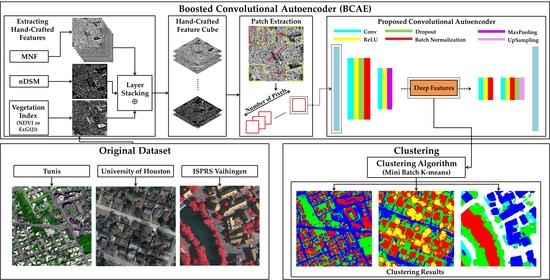
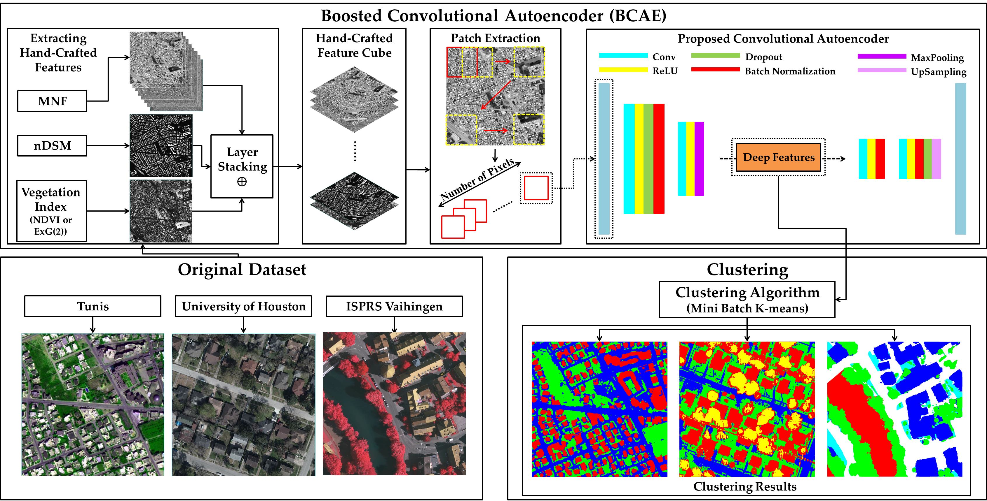
2.1. Remotely Sensed Data
- Tunis: These data are an improved satellite image in terms of spatial resolution by the Gram–Schmidt technique and includes eight spectral bands with a spatial resolution of 50 cm acquired by a WorldView-2 sensor. In terms of dimensions, this image is 809 × 809 pixels. This dataset includes digital terrain model (DTM) and digital surface model (DSM) of the study area;
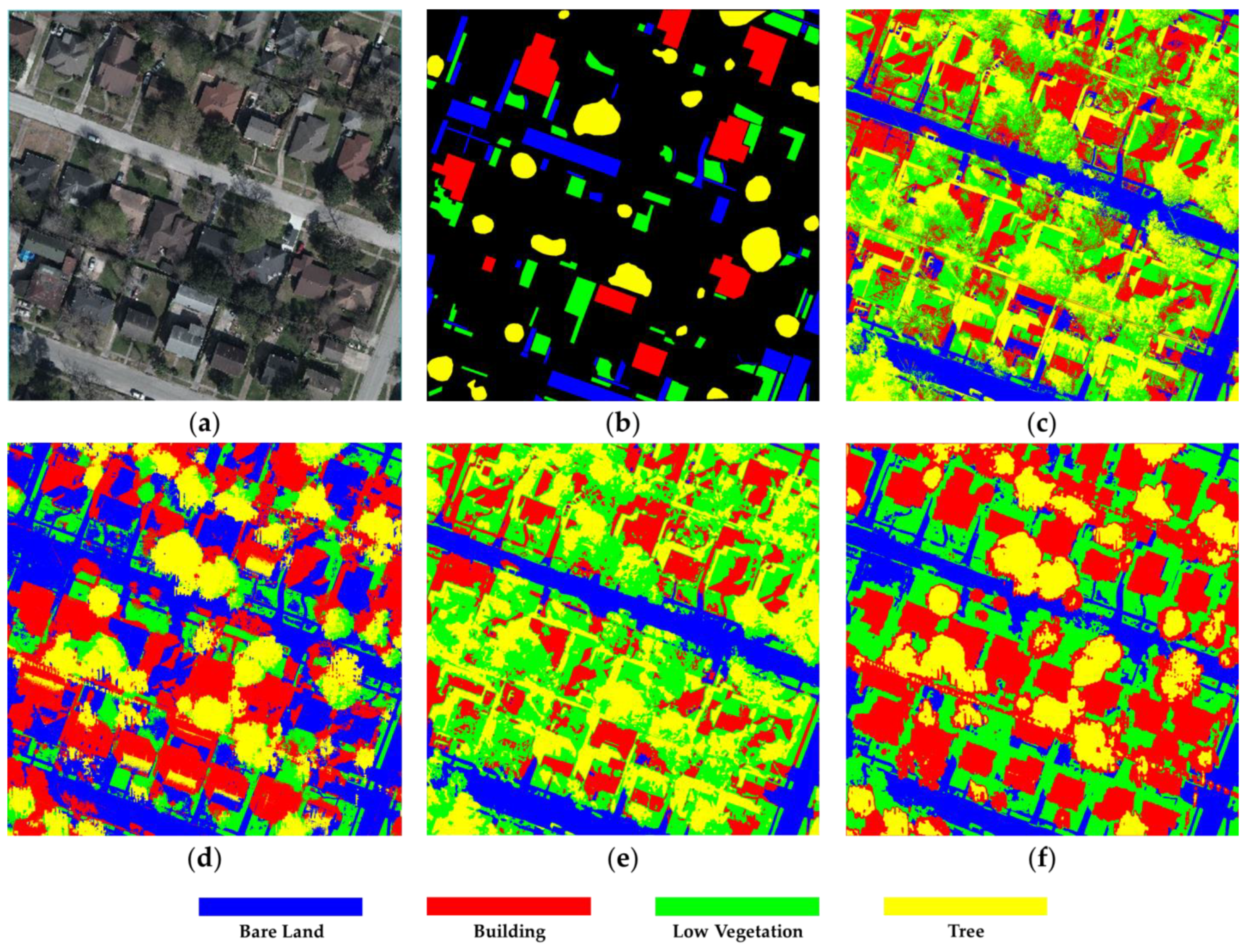
- University of Houston: The imagery was acquired by National Center for Airborne Laser Mapping (NCALM) on 16 February 2017. The recording sensors consist of an Optech Titan MW (14SEN/CON340) with an integrated camera (a LiDAR imager operating at 1550, 1064, and 532 nm) and a DiMAC ULTRALIGHT + (a very high-resolution color sensor) with a 70 mm focal length. We produced DTM and DSM from this dataset from multispectral LiDAR point cloud data at a 50 cm ground sample distance (GSD) and a very high-resolution RGB image at a 5 cm GSD. The data cube used in the study includes a crop of the original data with a width and height of 1500 × 1500 pixels, in 5 layers (blue, green, and red bands with DSM and DTM);
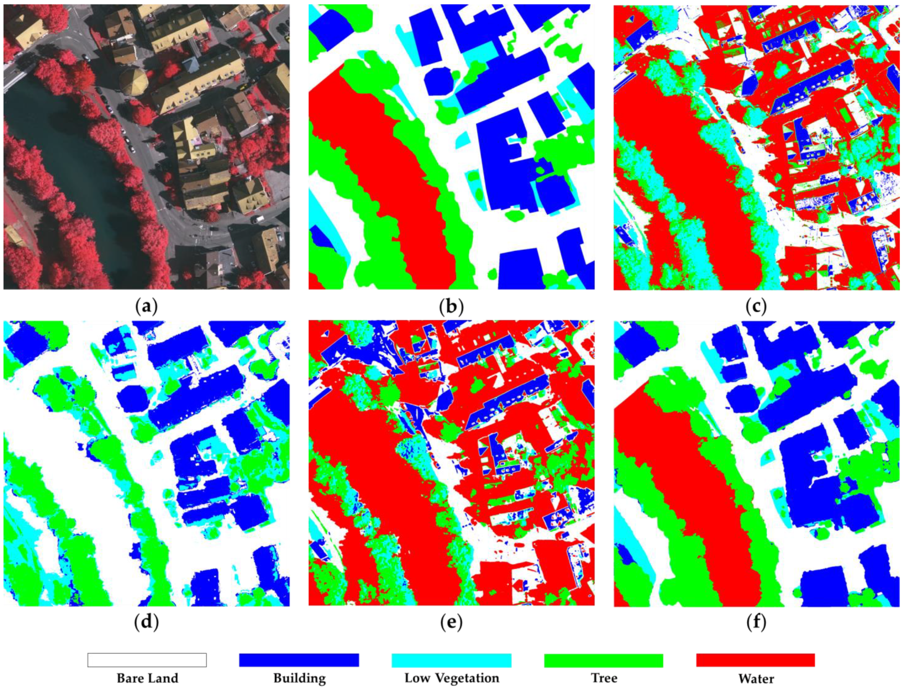
- ISPRS Vaihingen: The German Association of Photogrammetry, Remote Sensing, and Geoinformation produced the dataset. It consists of 33 image tiles in infra-red, red, and green wavelength and GSD of 9 cm/pixel that there is ground truth for 16 of them. This imagery also contains DSM extracted from dense LiDAR data. We used a 1500 × 1500 pixel cube from the 26th image patch in the dataset in 4 layers (IR-R-G with nDSM). It should be noted that we used the nDSM generated by Gerke [43].
2.2. Methodology
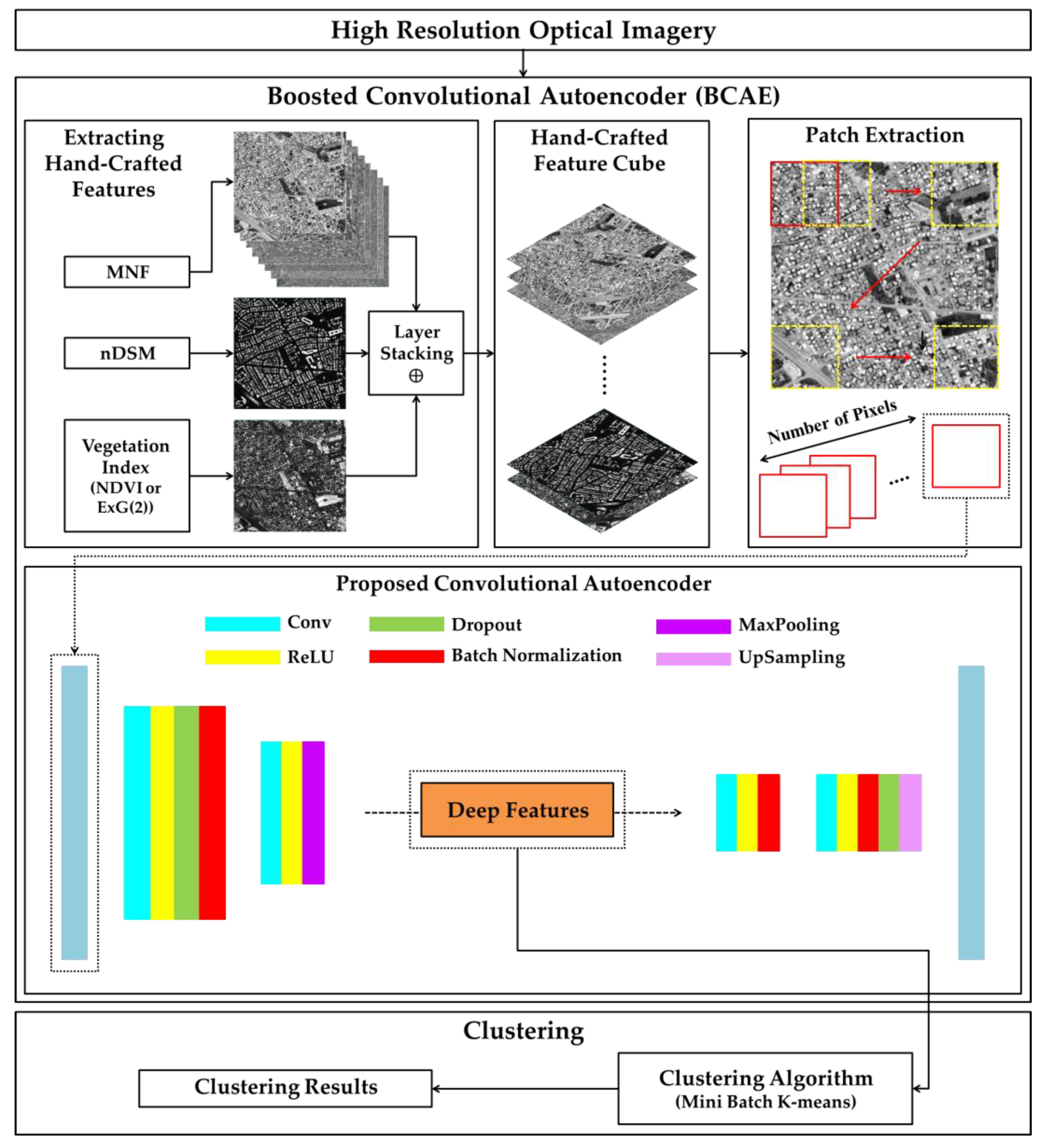
2.2.1. Boosted Convolutional Autoencoder (BCAE)
2.2.2. Boosting Deep Representations with Hand-crafted Features
2.3. Accuracy Assessment
2.4. Parameter Setting
2.5. Competing Features
- MS (Multispectral features);
- MDE (MNF + nDSM + ExG(2)) for UH dataset and MDN (MNF + nDSM + NDVI) for Tunis and Vaihingen datasets;
- CAE_MS.
2.6. Mini Batch K-Means
3. Experimental Results
3.1. Preprocessing
3.2. Clustering Results
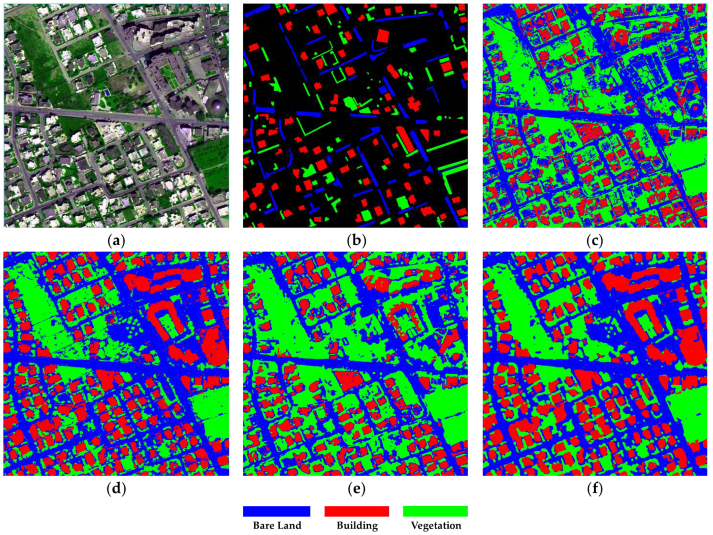
3.2.1. Tunis Dataset
3.2.2. UH Dataset
3.2.3. Vaihingen Dataset
3.2.4. Running Time Comparison
4. Discussion
5. Conclusions
Author Contributions
Funding
Institutional Review Board Statement
Informed Consent Statement
Data Availability Statement
Acknowledgments
Conflicts of Interest
References
- Basu, S.; Ganguly, S.; Mukhopadhyay, S.; DiBiano, R.; Karki, M.; Nemani, R. Deepsat: A learning framework for satellite imagery. In Proceedings of the 23rd ACM SIGSPATIAL International Conference on Advances in Geographic Information Systems, Seattle, WA, USA, 3–6 November 2015; pp. 1–10. [Google Scholar]
- Sheikholeslami, M.M.; Nadi, S.; Naeini, A.A.; Ghamisi, P. An Efficient Deep Unsupervised Superresolution Model for Remote Sensing Images. IEEE J. Sel. Top. Appl. Earth Obs. Remote Sens. 2020, 13, 1937–1945. [Google Scholar] [CrossRef]
- Naeini, A.A.; Babadi, M.; Homayouni, S. Assessment of Normalization Techniques on the Accuracy of Hyperspectral Data Clustering. In Proceedings of the International Archives of the Photogrammetry, Remote Sensing & Spatial Information Sciences, Tehran, Iran, 7–10 October 2017. [Google Scholar]
- Ghasedi Dizaji, K.; Herandi, A.; Deng, C.; Cai, W.; Huang, H. Deep clustering via joint convolutional autoencoder embedding and relative entropy minimization. In Proceedings of the 2017 IEEE International Conference on Computer Vision (ICCV), Venice, Italy, 22–29 October 2017; pp. 5736–5745. [Google Scholar]
- Fatemi, S.B.; Mobasheri, M.R.; Abkar, A.A. Clustering multispectral images using spatial-spectral information. IEEE Geosci. Remote Sens. Lett. 2015, 12, 1521–1525. [Google Scholar] [CrossRef]
- Mousavi, S.M.; Zhu, W.; Ellsworth, W.; Beroza, G. Unsupervised clustering of seismic signals using deep convolutional autoencoders. IEEE Geosci. Remote Sens. Lett. 2019, 16, 1693–1697. [Google Scholar] [CrossRef]
- Bengio, Y.; Courville, A.; Vincent, P. Representation learning: A review and new perspectives. IEEE Trans. Pattern Anal. Mach. Intell. 2013, 35, 1798–1828. [Google Scholar] [CrossRef]
- Fard, M.M.; Thonet, T.; Gaussier, E. Deep k-means: Jointly clustering with k-means and learning representations. Pattern Recognit. Lett. 2020, 138, 185–192. [Google Scholar] [CrossRef]
- Tao, C.; Pan, H.; Li, Y.; Zou, Z. Unsupervised spectral-spatial feature learning with stacked sparse autoencoder for hyperspectral imagery classification. IEEE Geosci. Remote Sens. Lett. 2015, 12, 2438–2442. [Google Scholar]
- Song, C.; Huang, Y.; Liu, F.; Wang, Z.; Wang, L. Deep auto-encoder based clustering. Intell. Data Anal. 2014, 18, S65–S76. [Google Scholar] [CrossRef]
- Cheng, G.; Han, J.; Lu, X. Remote sensing image scene classification: Benchmark and state of the art. Proc. IEEE 2017, 105, 1865–1883. [Google Scholar] [CrossRef] [Green Version]
- Hu, F.; Xia, G.-S.; Wang, Z.; Huang, X.; Zhang, L.; Sun, H. Unsupervised feature learning via spectral clustering of multidimensional patches for remotely sensed scene classification. IEEE J. Sel. Top. Appl. Earth Obs. Remote Sens. 2015, 8, 2015–2030. [Google Scholar] [CrossRef]
- Van De Sande, K.; Gevers, T.; Snoek, C. Evaluating color descriptors for object and scene recognition. IEEE Trans. Pattern Anal. Mach. Intell. 2009, 32, 1582–1596. [Google Scholar] [CrossRef]
- Guo, Z.; Zhang, L.; Zhang, D. A completed modeling of local binary pattern operator for texture classification. IEEE Trans. Image Process. 2010, 19, 1657–1663. [Google Scholar] [PubMed] [Green Version]
- Hong, S.; Choi, J.; Feyereisl, J.; Han, B.; Davis, L.S. Joint image clustering and labeling by matrix factorization. IEEE Trans. Pattern Anal. Mach. Intell. 2015, 38, 1411–1424. [Google Scholar] [CrossRef] [PubMed]
- Sampat, M.P.; Wang, Z.; Gupta, S.; Bovik, A.C.; Markey, M.K. Complex wavelet structural similarity: A new image similarity index. IEEE Trans. Image Process. 2009, 18, 2385–2401. [Google Scholar] [CrossRef]
- Kemker, R.; Salvaggio, C.; Kanan, C. Algorithms for semantic segmentation of multispectral remote sensing imagery using deep learning. ISPRS J. Photogramm. Remote Sens. 2018, 145, 60–77. [Google Scholar] [CrossRef] [Green Version]
- Pearson, K. LIII. On lines and planes of closest fit to systems of points in space. Lond. Edinb. Dubl. Phil. Mag. 1901, 2, 559–572. [Google Scholar] [CrossRef] [Green Version]
- Xing, C.; Ma, L.; Yang, X. Stacked denoise autoencoder based feature extraction and classification for hyperspectral images. J. Sens. 2016, 2016, 3632943. [Google Scholar] [CrossRef] [Green Version]
- Opochinsky, Y.; Chazan, S.E.; Gannot, S.; Goldberger, J. K-autoencoders deep clustering. In Proceedings of the ICASSP 2020–2020 IEEE International Conference on Acoustics, Speech and Signal Processing (ICASSP), Barcelona, Spain, 4–8 May 2020; pp. 4037–4041. [Google Scholar]
- Hamidi, M.; Safari, A.; Homayouni, S. An auto-encoder based classifier for crop mapping from multitemporal multispectral imagery. Int. J. Remote Sens. 2021, 42, 986–1016. [Google Scholar] [CrossRef]
- Song, C.; Liu, F.; Huang, Y.; Wang, L.; Tan, T. Auto-encoder based data clustering. In Proceedings of the 2013 Iberoamerican Congress on Pattern Recognition, Havana, Cuba, 20–23 November 2013; pp. 117–124. [Google Scholar]
- Chen, P.-Y.; Huang, J.-J. A hybrid autoencoder network for unsupervised image clustering. Algorithms 2019, 12, 122. [Google Scholar] [CrossRef] [Green Version]
- Huang, P.; Huang, Y.; Wang, W.; Wang, L. Deep embedding network for clustering. In Proceedings of the 2014 22nd International Conference on Pattern Recognition, Stockholm, Sweden, 24–28 August 2014; pp. 1532–1537. [Google Scholar]
- Tian, F.; Gao, B.; Cui, Q.; Chen, E.; Liu, T.-Y. Learning deep representations for graph clustering. In Proceedings of the 28th AAAI Conference on Artificial Intelligence, Québec City, QC, Canada, 27–31 July 2014; pp. 1293–1299. [Google Scholar]
- Yang, B.; Fu, X.; Sidiropoulos, N.D.; Hong, M. Towards k-means-friendly spaces: Simultaneous deep learning and clustering. In Proceedings of the 34th International Conference on Machine Learning, Sydney, Australia, 6–11 August 2017; pp. 3861–3870. [Google Scholar]
- Xie, J.; Girshick, R.; Farhadi, A. Unsupervised deep embedding for clustering analysis. In Proceedings of the 33rd International Conference on Machine Learning, New York, NY, USA, 19–24 June 2016; pp. 478–487. [Google Scholar]
- Guo, X.; Gao, L.; Liu, X.; Yin, J. Improved deep embedded clustering with local structure preservation. In Proceedings of the IJCAI 26th International Joint Conference on Artificial Intelligence, Melbourne, Australia, 19–25 August 2017; pp. 1753–1759. [Google Scholar]
- Guo, X.; Liu, X.; Zhu, E.; Yin, J. Deep clustering with convolutional autoencoders. In Proceedings of the 24th International Conference on Neural Information Processing, Guangzhou, China, 14–18 November 2017; pp. 373–382. [Google Scholar]
- Li, F.; Qiao, H.; Zhang, B. Discriminatively boosted image clustering with fully convolutional auto-encoders. Pattern Recognit. 2018, 83, 161–173. [Google Scholar] [CrossRef] [Green Version]
- Krizhevsky, A.; Sutskever, I.; Hinton, G.E. Imagenet classification with deep convolutional neural networks. In Proceedings of the Advances in Neural Information Processing Systems 25: 26th Annual Conference on Neural Information Processing Systems, Lake Tahoe, NV, USA, 3–6 December 2012; pp. 1097–1105. [Google Scholar]
- Wang, S.; Cao, J.; Yu, P. Deep learning for spatio-temporal data mining: A survey. IEEE Trans. Knowl. Data Eng. 2020. [Google Scholar] [CrossRef]
- Affeldt, S.; Labiod, L.; Nadif, M. Spectral clustering via ensemble deep autoencoder learning (SC-EDAE). Pattern Recognit. 2020, 108, 107522. [Google Scholar] [CrossRef]
- Paisitkriangkrai, S.; Sherrah, J.; Janney, P.; Van Den Hengel, A. Semantic labeling of aerial and satellite imagery. IEEE J. Sel. Top. Appl. Earth Obs. Remote Sens. 2016, 9, 2868–2881. [Google Scholar] [CrossRef]
- Nijhawan, R.; Das, J.; Raman, B. A hybrid of deep learning and hand-crafted features based approach for snow cover mapping. Int. J. Remote Sens. 2019, 40, 759–773. [Google Scholar] [CrossRef]
- Majtner, T.; Yildirim-Yayilgan, S.; Hardeberg, J.Y. Combining deep learning and hand-crafted features for skin lesion classification. In Proceedings of the 2016 Sixth International Conference on Image Processing Theory, Tools and Applications (IPTA), Oulu, Finland, 12–15 December 2016; pp. 1–6. [Google Scholar]
- TaSci, E.; Ugur, A. Image classification using ensemble algorithms with deep learning and hand-crafted features. In Proceedings of the 2018 26th Signal Processing and Communications Applications Conference (SIU), Izmir, Turkey, 2–5 May 2018; pp. 1–4. [Google Scholar]
- Hong, D.; Gao, L.; Yokoya, N.; Yao, J.; Chanussot, J.; Du, Q.; Zhang, B. More diverse means better: Multimodal deep learning meets remote-sensing imagery classification. IEEE Trans. Geosci. Remote Sens. 2021, 59, 4340–4354. [Google Scholar] [CrossRef]
- Chen, Y.; Li, C.; Ghamisi, P.; Jia, X.; Gu, Y. Deep fusion of remote sensing data for accurate classification. IEEE Geosci. Remote Sens. Lett. 2017, 14, 1253–1257. [Google Scholar] [CrossRef]
- Hang, R.; Liu, Q.; Hong, D.; Ghamisi, P. Cascaded recurrent neural networks for hyperspectral image classification. IEEE Trans. Geosci. Remote Sens. 2019, 57, 5384–5394. [Google Scholar] [CrossRef] [Green Version]
- Ienco, D.; Gbodjo, Y.J.E.; Gaetano, R.; Interdonato, R. Generalized Knowledge Distillation for Multi-Sensor Remote Sensing Classification: AN Application to Land Cover Mapping. In Proceedings of the ISPRS Annals of the Photogrammetry, Remote Sensing and Spatial Information Sciences, Nice, France, 31 August-2 September 2020; pp. 997–1003. [Google Scholar]
- Aghdam, H.H.; Heravi, E.J. Guide to Convolutional Neural Networks; Springer: New York, NY, USA, 2017; Volume 282, p. 7. [Google Scholar]
- Gerke, M. Use of the Stair Vision Library within the ISPRS 2D Semantic Labeling Benchmark (Vaihingen); Technical Report; University of Twente: Enschede, The Netherlands, 2014. [Google Scholar]
- Green, A.A.; Berman, M.; Switzer, P.; Craig, M.D. A transformation for ordering multispectral data in terms of image quality with implications for noise removal. IEEE Trans. Geosci. Remote Sens. 1988, 26, 65–74. [Google Scholar] [CrossRef] [Green Version]
- Masci, J.; Meier, U.; Cireşan, D.; Schmidhuber, J. Stacked convolutional auto-encoders for hierarchical feature extraction. In Proceedings of the International Conference on Artificial Neural Networks, Espoo, Finland, 14–17 June 2011; pp. 52–59. [Google Scholar]
- Tang, X.; Zhang, X.; Liu, F.; Jiao, L. Unsupervised deep feature learning for remote sensing image retrieval. Remote Sens. 2018, 10, 1243. [Google Scholar] [CrossRef] [Green Version]
- Ribeiro, M.; Lazzaretti, A.E.; Lopes, H.S. A study of deep convolutional auto-encoders for anomaly detection in videos. Pattern Recognit. Lett. 2018, 105, 13–22. [Google Scholar] [CrossRef]
- Zhao, W.; Guo, Z.; Yue, J.; Zhang, X.; Luo, L. On combining multiscale deep learning features for the classification of hyperspectral remote sensing imagery. Int. J. Remote Sens. 2015, 36, 3368–3379. [Google Scholar] [CrossRef]
- Othman, E.; Bazi, Y.; Alajlan, N.; Alhichri, H.; Melgani, F. Using convolutional features and a sparse autoencoder for land-use scene classification. Int. J. Remote Sens. 2016, 37, 2149–2167. [Google Scholar] [CrossRef]
- Kingma, D.P.; Ba, J. Adam: A method for stochastic optimization. arXiv 2014, arXiv:1412.6980. [Google Scholar]
- Srivastava, N.; Hinton, G.; Krizhevsky, A.; Sutskever, I.; Salakhutdinov, R. Dropout: A simple way to prevent neural networks from overfitting. J. Mach. Learn. Res. 2014, 15, 1929–1958. [Google Scholar]
- Zhu, X.X.; Tuia, D.; Mou, L.; Xia, G.-S.; Zhang, L.; Xu, F.; Fraundorfer, F. Deep learning in remote sensing: A comprehensive review and list of resources. IEEE Geosci. Remote Sens. Mag. 2017, 5, 8–36. [Google Scholar] [CrossRef] [Green Version]
- Ioffe, S.; Szegedy, C. Batch normalization: Accelerating deep network training by reducing internal covariate shift. arXiv 2015, arXiv:1502.03167. [Google Scholar]
- Chen, Y.; Wang, Y.; Gu, Y.; He, X.; Ghamisi, P.; Jia, X. Deep learning ensemble for hyperspectral image classification. IEEE J. Sel. Top. Appl. Earth Obs. Remote Sens. 2019, 12, 1882–1897. [Google Scholar] [CrossRef]
- Huang, M.-J.; Shyue, S.-W.; Lee, L.-H.; Kao, C.-C. A knowledge-based approach to urban feature classification using aerial imagery with lidar data. Photogramm. Eng. Remote Sens. 2008, 74, 1473–1485. [Google Scholar] [CrossRef] [Green Version]
- Man, Q.; Dong, P.; Guo, H. Pixel-and feature-level fusion of hyperspectral and lidar data for urban land-use classification. Int. J. Remote Sens. 2015, 36, 1618–1644. [Google Scholar] [CrossRef]
- Rottensteiner, F.; Sohn, G.; Gerke, M.; Wegner, J.D.; Breitkopf, U.; Jung, J. Results of the ISPRS benchmark on urban object detection and 3D building reconstruction. ISPRS J. Photogramm. Remote Sens. 2014, 93, 256–271. [Google Scholar] [CrossRef]
- Rafiezadeh Shahi, K.; Ghamisi, P.; Rasti, B.; Jackisch, R.; Scheunders, P.; Gloaguen, R. Data Fusion Using a Multi-Sensor Sparse-Based Clustering Algorithm. Remote Sens. 2020, 12, 4007. [Google Scholar] [CrossRef]
- Hartfield, K.A.; Landau, K.I.; Van Leeuwen, W.J. Fusion of high resolution aerial multispectral and LiDAR data: Land cover in the context of urban mosquito habitat. Remote Sens. 2011, 3, 2364–2383. [Google Scholar] [CrossRef] [Green Version]
- Gevaert, C.; Persello, C.; Sliuzas, R.; Vosselman, G. Informal settlement classification using point-cloud and image-based features from UAV data. ISPRS J. Photogramm. Remote Sens. 2017, 125, 225–236. [Google Scholar] [CrossRef]
- MacFaden, S.W.; O’Neil-Dunne, J.P.; Royar, A.R.; Lu, J.W.; Rundle, A.G. High-resolution tree canopy mapping for New York City using LIDAR and object-based image analysis. J. Appl. Remote Sens. 2012, 6, 063567. [Google Scholar] [CrossRef]
- Torres-Sánchez, J.; Pena, J.M.; de Castro, A.I.; López-Granados, F. Multi-temporal mapping of the vegetation fraction in early-season wheat fields using images from UAV. Comput. Electron. Agric. 2014, 103, 104–113. [Google Scholar] [CrossRef]
- Woebbecke, D.M.; Meyer, G.E.; Von Bargen, K.; Mortensen, D.A. Color indices for weed identification under various soil, residue, and lighting conditions. Trans. ASAE 1995, 38, 259–269. [Google Scholar] [CrossRef]
- Denghui, Z.; Le, Y. Support vector machine based classification for hyperspectral remote sensing images after minimum noise fraction rotation transformation. In Proceedings of the 2011 International Conference on Internet Computing and Information Services, Hong Kong, China, 17–18 September 2011; pp. 132–135. [Google Scholar]
- Lixin, G.; Weixin, X.; Jihong, P. Segmented minimum noise fraction transformation for efficient feature extraction of hyperspectral images. Pattern Recognit. 2015, 48, 3216–3226. [Google Scholar] [CrossRef]
- Li, H.; Zhang, S.; Ding, X.; Zhang, C.; Dale, P. Performance evaluation of cluster validity indices (CVIs) on multi/hyperspectral remote sensing datasets. Remote Sens. 2016, 8, 295. [Google Scholar] [CrossRef] [Green Version]
- Hanhijärvi, S.; Ojala, M.; Vuokko, N.; Puolamäki, K.; Tatti, N.; Mannila, H. Tell me something I don’t know: Randomization strategies for iterative data mining. In Proceedings of the 15th ACM SIGKDD International Conference on Knowledge Discovery and Data Mining, Paris, France, 28 June–1 July 2009; pp. 379–388. [Google Scholar]
- Seydgar, M.; Alizadeh Naeini, A.; Zhang, M.; Li, W.; Satari, M. 3-D convolution-recurrent networks for spectral-spatial classification of hyperspectral images. Remote Sens. 2019, 11, 883. [Google Scholar] [CrossRef] [Green Version]
- Sculley, D. Web-scale k-means clustering. In Proceedings of the 19th International Conference on World Wide Web, Raleigh, NC, USA, 26–30 April 2010; pp. 1177–1178. [Google Scholar]
- Feizollah, A.; Anuar, N.B.; Salleh, R.; Amalina, F. Comparative study of k-means and mini batch k-means clustering algorithms in android malware detection using network traffic analysis. In Proceedings of the 2014 International Symposium on Biometrics and Security Technologies (ISBAST), Kuala Lumpur, Malaysia, 26–27 August 2014; pp. 193–197. [Google Scholar]
- Béjar Alonso, J. K-Means vs Mini Batch K-Means: A Comparison; (Technical Report); Universitat Poiltecnica de Catalunya: Barcelona, Spain, 2013. [Google Scholar]
- Yan, B.; Zhang, Y.; Yang, Z.; Su, H.; Zheng, H. DVT-PKM: An improved GPU based parallel k-means algorithm. In Proceedings of the 2014 International Conference on Intelligent Computing, Taiyuan, China, 3–6 August 2014; pp. 591–601. [Google Scholar]


| Feature | Definition |
|---|---|
| nDSM | nDSM = DSM – DTM where DSM is the digital surface model, and DTM is the digital terrain model. |
| NDVI | where is the reflectance of the near-infrared wavelength band and is the reflectance of the red wavelength band. |
| ExG(2) | where r, g, and b are the color band divided by the sum of three bands per pixel [60]. |
| MNF | Considering noisy data as with -bands in the form of , where and are the signals and noise parts of , the covariance matrices of and can be calculated as follow: Then, the noise variance of the band with respect to the variance for band can be described as: In the following, the MNF transform is considered as a linear transformation: where, y is a produced dataset with bands, which is a transformation of the original bands, the unknown coefficients are obtained by calculating the eigenvectors associated with sorted eigenvalues: where, is eigenvalue matrix , each eigenvalue associated with is the noise ratio in [65]. |
| Class | Ground Truth (Pixel) |
|---|---|
| Bare Land | 39,052 |
| Building | 48,909 |
| Vegetation | 33,499 |
| Total | 121,460 |
| Class | Ground Truth (Pixel) |
|---|---|
| Bare Land | 131,061 |
| Building | 133,856 |
| Low Vegetation | 135,513 |
| Tree | 137,151 |
| Total | 537,581 |
| Class | Ground Truth (Pixel) |
|---|---|
| Bare Land | 719,721 |
| Building | 534,190 |
| Low Vegetation | 128,787 |
| Tree | 508,345 |
| Water | 358,957 |
| Total | 2,250,000 |
| Block | Unit | Input Shape | Kernel Size | Regularization | Output Shape |
|---|---|---|---|---|---|
| Encoder | CNN1 + ReLU + BN | 7 × 7 × D | 3 × 3 | Dropout (30%) | 5 × 5 × 12 |
| CNN2 + ReLU + BN | 5 × 5 × 12 | 3 × 3 | - | 3 × 3 × 24 | |
| MaxPooling | 3 × 3 × 24 | 2 × 2 | - | 1 × 1 × 24 | |
| Decoder | CNN3 + ReLU + BN | 1 × 1 × 24 | 1 × 1 | 1 × 1 × 12 | |
| CNN4 + ReLU + BN | 1 × 1 × 12 | 1 × 1 | Dropout (30%) | 1 × 1 × D | |
| UpSampling | 1 × 1 × D | 7 × 7 | - | 7 × 7 × D |
| Preprocessing | Dataset | |||
|---|---|---|---|---|
| UH | Tunis | Vaihingen | ||
| Features Extraction | MNF | ☑ | ☑ | ☑ |
| nDSM | ☑ | ☑ | ☑ | |
| NDVI | - | ☑ | ☑ | |
| ExG(2) | ☑ | - | - | |
| Dataset | MNF Transformation Results |
|---|---|
| Tunis |  |
| UH |  |
| Vaihingen | 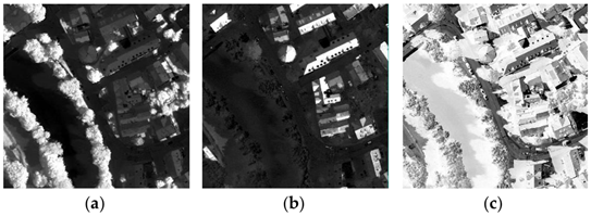 |
| Dataset | MNF Band | Eigenvalue | Variance | |
|---|---|---|---|---|
| Per Band (%) | Accumulative (%) | |||
| Tunis | 1 | 85.4706 | 34.99 | 34.9 |
| 2 | 53.9577 | 22.09 | 57.08 | |
| 3 | 27.5616 | 11.29 | 68.37 | |
| 4 | 22.4381 | 9.18 | 77.55 | |
| 5 | 17.8637 | 7.32 | 84.87 | |
| 6 | 16.7731 | 6.86 | 91.73 | |
| 7 | 14.9745 | 6.13 | 97.86 | |
| 8 | 5.2181 | 2.14 | 100.00 | |
| UH | 1 | 97.7494 | 46.72 | 46.72 |
| 2 | 64.9348 | 31.03 | 77.75 | |
| 3 | 46.5552 | 22.25 | 100.00 | |
| Vaihingen | 1 | 219.6756 | 55.69 | 55.69 |
| 2 | 128.2491 | 34.10 | 89.79 | |
| 3 | 39.5643 | 10.21 | 100.00 | |
| Class (Producer’s/User’s Accuracy (%)) | Method | |||
|---|---|---|---|---|
| MS | MDN | CAE–MS | BCAE | |
| Bare Land | 90.77/63.40 | 97.46/77.10 | 92.02/77.72 | 98.32/85.96 |
| Building | 41.90/92.19 | 81.71/99.43 | 55.93/99.17 | 87.94/99.54 |
| Vegetation | 98.32/76.02 | 91.33/95.91 | 98.42/69.21 | 97.83/97.59 |
| Overall Accuracy | 73.17 | 89.43 | 79.25 | 94.01 |
| Kappa Coefficient (×100) | 60.54 | 84.07 | 69.40 | 90.95 |
| Class (Producer’s/User’s Accuracy (%)) | Method | |||
|---|---|---|---|---|
| MS | MDN | CAE–MS | BCAE | |
| Bare Land | 79.43/93.56 | 94.35/79.18 | 75.65/93.01 | 94.29/96.70 |
| Building | 45.35/54.82 | 50.09/89.04 | 54.54/59.88 | 96.59/77.84 |
| Low Vegetation | 66.82/43.40 | 77.33/64.06 | 71.63/43.76 | 94.21/94.58 |
| Tree | 38.76/49.71 | 68.27/39.39 | 32.93/51.77 | 77.37/97.61 |
| Overall Accuracy | 55.64 | 67.87 | 58.48 | 90.53 |
| Kappa Coefficient (×100) | 40.85 | 57.23 | 44.62 | 87.37 |
| Class (Producer’s/User’s Accuracy (%)) | Method | |||
|---|---|---|---|---|
| MS | MDN | CAE–MS | BCAE | |
| Bare Land | 40.28/65.12 | 94.16/32.46 | 34.21/61.60 | 91.63/97.22 |
| Building | 23.46/85.63 | 76.23/86.03 | 23.27/60.57 | 94.96/90.48 |
| Low Vegetation | 51.79/85.97 | 50.53/21.56 | 9.34/8.72 | 74.67/77.24 |
| Tree | 10.82/5.08 | 75.17/88.12 | 51.09/81.75 | 93.73/90.79 |
| Water | 98.00/32.64 | 00.00/00.00 | 98.24/29.65 | 97.52/96.79 |
| Overall Accuracy | 46.41 | 53.00 | 44.22 | 92.86 |
| Kappa Coefficient (×100) | 33.60 | 43.03 | 30.43 | 90.65 |
| Method | UH (s) | Tunis (s) | Vaihingen (s) |
|---|---|---|---|
| MS | 34.542 | 11.063 | 40.146 |
| MDE/MDN | 33.379 | 10.486 | 48.911 |
| CAE–MS | 39.755 | 9.917 | 37.345 |
| BCAE | 31.292 | 9.864 | 35.308 |
Publisher’s Note: MDPI stays neutral with regard to jurisdictional claims in published maps and institutional affiliations. |
© 2021 by the authors. Licensee MDPI, Basel, Switzerland. This article is an open access article distributed under the terms and conditions of the Creative Commons Attribution (CC BY) license (https://creativecommons.org/licenses/by/4.0/).
Share and Cite
Rahimzad, M.; Homayouni, S.; Alizadeh Naeini, A.; Nadi, S. An Efficient Multi-Sensor Remote Sensing Image Clustering in Urban Areas via Boosted Convolutional Autoencoder (BCAE). Remote Sens. 2021, 13, 2501. https://doi.org/10.3390/rs13132501
Rahimzad M, Homayouni S, Alizadeh Naeini A, Nadi S. An Efficient Multi-Sensor Remote Sensing Image Clustering in Urban Areas via Boosted Convolutional Autoencoder (BCAE). Remote Sensing. 2021; 13(13):2501. https://doi.org/10.3390/rs13132501
Chicago/Turabian StyleRahimzad, Maryam, Saeid Homayouni, Amin Alizadeh Naeini, and Saeed Nadi. 2021. "An Efficient Multi-Sensor Remote Sensing Image Clustering in Urban Areas via Boosted Convolutional Autoencoder (BCAE)" Remote Sensing 13, no. 13: 2501. https://doi.org/10.3390/rs13132501
APA StyleRahimzad, M., Homayouni, S., Alizadeh Naeini, A., & Nadi, S. (2021). An Efficient Multi-Sensor Remote Sensing Image Clustering in Urban Areas via Boosted Convolutional Autoencoder (BCAE). Remote Sensing, 13(13), 2501. https://doi.org/10.3390/rs13132501